Implementation of an ensemble Kalman filter in the Community Multiscale Air Quality model (CMAQ model v5.1) for data assimilation of ground-level PM_2.5

In this study, we developed a data assimilation (DA) system for chemical transport model (CTM) simulations using an ensemble Kalman filter (EnKF) technique. This DA technique is easy to implement in an existing system without seriously modifying the original CTM and can provide flow-dependent corrections based on error covariance by short-term ensemble propagations. First, the PM_2.5 observations at ground stations were assimilated in this DA system every 6 h over South Korea for the period of the KORUS–AQ campaign from 1 May to 12 June 2016. The DA performances with the EnKF were then compared to a control run (CTR) without DA and a run with three-dimensional variational (3D-Var) DA. Consistent improvements owing to the initial conditions (ICs) assimilated with the EnKF were found in the DA experiments at a 6 h interval compared to the CTR run and to the run with 3D-Var. In addition, we attempted to assimilate the ground observations from China to examine the impacts of improved boundary conditions (BCs) on the PM_2.5 predictability over South Korea. The contributions of the ICs and BCs to improvements in the PM_2.5 predictability were also quantified. For example, the relative reductions in terms of the normalized mean bias (NMB) were found to be approximately 27.2 % for the 6 h reanalysis run. A series of 24 h PM_2.5 predictions were additionally conducted each day at 00:00 UTC with the optimized ICs. The relative reduction of the NMB was 17.3 % for the 24 h prediction run when the updated ICs were applied at 00:00 UTC. This means that after the application of the updated BCs, an additional 9.0 % reduction in the NMB was achieved for 24 h PM_2.5 predictions in South Korea.

1 Introduction

Among many air pollutants, particular attention has been paid to the issue of atmospheric aerosols in East Asia and South Korea, where large anthropogenic emissions from growing economic activities cause frequent episodes of high air pollution. Several environmental and epidemiological studies have suggested that continual exposure to particulate matter with aerodynamic diameter smaller than 2.5 µm (PM_2.5) has critical effects on human mortality and morbidity (Pope and Dockery, 2006; Cohen et al., 2017; Dehghani et al., 2017). Because of the severity of the influences of PM_2.5 on human health, the accuracy of PM_2.5 forecasts has become a central issue in South Korea. To achieve the goal of improving PM_2.5 predictability, the National Institute of Environmental Research (NIER) of South Korea has implemented daily operational air quality forecast since 2014 using a 3-D chemical transport model (CTM) (Chang et al., 2016), while the Korean Ministry of the Environment (KMoE) provides real-time observations of PM_2.5, together with the concentrations of five other criteria air pollutants (PM₁₀, O₃, CO, SO₂, and NO₂) via a website named “Air Korea” (https://www.airkorea.or.kr, last access: 22 March 2022​​​​​​​). Although in general the CTM simulation can overcome the spatial and temporal limitations of ground observations, it has large uncertainties that are due to imperfect emissions, initial conditions (ICs), boundary conditions (BCs), meteorological fields, and physical and photochemical mechanisms (Carmichael et al., 2008; Solazzo et al., 2012).

To improve the accuracy of short-term predictions via CTM simulations, chemical data assimilation (DA) has been proposed as an effective method to reduce the uncertainties in the CTM parameters (e.g., Sandu and Chai, 2011; Zhang et al., 2012a, b; Bocquet et al., 2015; Menut and Bessagnet, 2019). Chemical DA is a technique for integrating information provided by noisy observations and imperfect background estimations from CTM simulations. This integration of the two groups of information can theoretically better represent the true state of the chemical atmosphere. DA techniques have been predominantly applied in the numerical weather prediction (NWP) (Kalnay, 2002), such as optimal interpolation (OI: Lorenc, 1981), the three-dimensional variational method (3D-Var: Lorenc, 1986; Parrish and Derber, 1992; Rabier et al., 1998), the four-dimensional variational method (4D-Var: Talagrand and Courtier, 1987; Courtier et al., 1994; Rabier et al., 2000), and the ensemble Kalman filter (EnKF: Evensen, 2003). While the utilization of DA techniques in air quality predictions has been limited, these techniques have more recently started to be used for air quality prediction as well. To date, several DA methods have been applied to optimize the uncertainties in model input parameters, including ICs (e.g., Elbern and Schmidt, 2001; Park et al., 2016), BCs (e.g., Roustan and Bocquet, 2006), and emission fluxes (e.g., Elbern et al., 2007).

For the past 2 decades, various DA algorithms have been applied, especially to aerosol prediction studies. Several studies have focused on assimilating aerosol observations via OI (Lee et al., 2013; Park et al., 2011, 2014; Tang et al., 2015, 2017; Chai et al., 2017; Lee et al., 2020​​​​​​​), 3D-Var (Pagowski et al., 2010; Liu et al., 2011; Schwartz et al., 2012; Saide et al., 2013; Jiang et al., 2013; Li et al., 2013; Pang et al., 2018; Ha et al., 2020), and 4D-Var (Benedetti et al., 2019; Morcrette et al., 2009). All the previous studies mentioned above have reported that the OI, 3D-Var, and 4D-Var assimilations using satellite-retrieved or ground-based observations led to improved aerosol predictability.

Even so, each of these DA methods has its own limitations. OI and 3D-Var usually employ isotropic corrections due to a static (i.e., time-invariant) background error covariance (BEC) based on model climatological profiles. Although 4D-Var has been reported to show better performance than OI and 3D-Var, it requires constant development and maintenance of a tangent linear and adjoint model, which may be a time-consuming and labor-intensive task (Skachko et al., 2014). On the other hand, EnKF is relatively easy to implement without requiring a tangent linear or adjoint model and can easily compute flow-dependent BEC from short-term ensemble predictions. This flow dependence of the BEC is one of the main reasons behind the possible success of the EnKF method compared to other DA methods. Several studies (Tang et al., 2011; Pagowski and Grell, 2012; Yumimoto and Takemura, 2015; Rubin et al., 2016; Yumimoto et al., 2016; Peng et al., 2017, 2018; Lopez-Restrepo et al., 2020) applied the EnKF DA approach to improve the accuracy of air quality prediction via assimilating surface and/or satellite observations. For example, Yumimoto et al. (2016) applied the EnKF method with satellite-retrieved aerosol observations to evaluate the effectiveness of the DA on dust forecasts and found improved agreement between the predictions and observations. More recently, Peng et al. (2017) reported significant improvements in PM_2.5 prediction via the joint optimization of ICs and emissions using the EnKF method by assimilating ground-based PM_2.5.

To optimize the ICs, two studies (Lin et al., 2008; Candiani et al., 2013) carried out assimilation using ground-based aerosol observations with different variants of EnKF DA algorithms. However, few studies have applied the EnKF method to examine the importance of BCs. When long-range transport is an important issue, BCs can provide important information. For example, Constantinescu et al. (2007a) extended the EnKF method to consider lateral BCs and correct emission flux factors in the assimilation process by solving the state parameter estimation problem. Other than this study, no prior study has applied the EnKF method to this type of research, particularly with the Community Multiscale Air Quality (CMAQ) model.

This work is a new endeavor to develop an EnKF DA system for the CMAQ model. The period of the KORUS–AQ campaign 2016 (1 May to 11 June 2016) was chosen to be the target period to test the developed EnKF DA system, since this period includes well-defined and various types of air pollution episodes, e.g., yellow dust events, stagnant high-PM episodes, long-range transport events, and rainy days (Peterson et al., 2019; Jordan et al., 2020). To improve the predictability of PM_2.5 in South Korea for this period, ground-based PM_2.5 data were assimilated to update the IC and BC fields. Since this is our first attempt to develop an EnKF DA system, we also compared the performances of the EnKF DA system with the existing 3D-Var DA algorithm (Lee et al., 2022).

We believe that this study can be distinguishable from other EnKF studies in three aspects: (i) the EnKF chemical DA system was first developed to assimilate PM_2.5 for or with the CMAQ model. In particular, this study intended to enhance the accuracy of PM_2.5 prediction via assimilating ground-observed PM_2.5 in South Korea (nearly 150 stations) and China (nearly 850 stations). The advantages of the assimilation of ground-observed PM_2.5 are also discussed in the text. (ii) The first developed EnKF DA system was applied to PM_2.5 predictions in South Korea, where air quality is frequently influenced by long-range transport from the eastern, northern, and northeastern parts of China (EC, NC, and NEC in Fig. 1). (iii) To evaluate the influences of inflow from China on air quality in South Korea more quantitatively, this study assimilated the ground observations from China and South Korea separately.

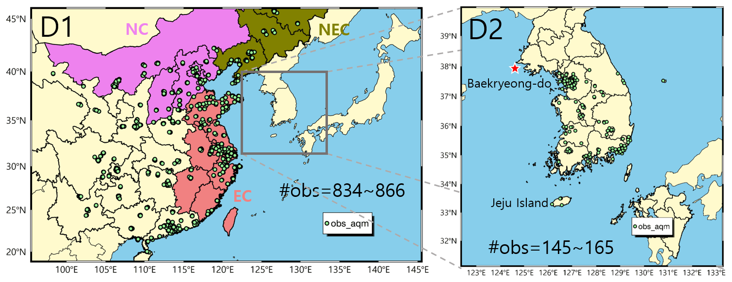
Figure 1 Simulation domains with nested modeling. D1 and D2 represent the mother and daughter domain, respectively. The locations of ground stations in China (D1) and South Korea (D2) are marked on the maps with green dots. In D1 (left), the northeastern China (NEC), northern China (NC), and eastern China (EC) regions that frequently influence air quality in South Korea are grouped with olive, violet, and coral colors, respectively. The red star symbol indicates Baekryeong-do observatory, where the evaluation of boundary inflow was made. Jeju Island in D2 (right) is an ideal location to see the flow-dependent correction by the EnKF DA. The total number of available stations used in EnKF data assimilation is also shown in both domains.

The remainder of this paper is organized as follows. Section 2 describes the methodology of this study, including the DA algorithm, CTM, observations, and experimental settings. Section 3.1 discusses the effects of assimilation of ground-based observations and then compares the results with those from 3D-Var based on the reanalysis results. Section 3.2 provides the results of improved BCs in 1 d prediction simulations. Section 3.3 quantifies the contributions of updating ICs and BCs with statistical analysis. Finally, Sect. 4 concludes the paper.

2 Methods

2.1 Ensemble Kalman filter (EnKF)

The EnKF is a DA technique first introduced by Evensen (1994), which was an approximate version of the Kalman filter (KF) (Kalman, 1960). The basic principle of the KF is to estimate a true state, while minimizing the variances of the state with a linear combination of the best estimates of the model and the observations. The optimal state estimated from the KF shows less uncertainty than the model predictions and observations. This optimal state is called the “analysis”. To apply the KF to a nonlinear model, a tangent linear model needs to be constructed, as does its adjoint. However, the EnKF requires neither a tangent linear model nor its adjoint, since it employs Monte Carlo approximation that can estimate the model error covariances using finite ensemble simulations (Evensen, 1994). In particular, the model error covariances used in the EnKF technique are flow-dependent, which is one of the major differences from other DA methods.

The theoretical foundation of the EnKF method proposed by Evensen (2003) is briefly presented below.

$$\begin{array}{}\text{(1)}& {\displaystyle }{\mathit{x}}_{i,k}^{\mathrm{f}}=\mathcal{M}{\mathit{x}}_{i,k-\mathrm{1}}^{\mathrm{a}}+{\mathit{q}}_{i,k},i=\mathrm{1},\mathrm{2},\mathrm{\dots },N\text{(2)}& {\displaystyle }{\mathit{y}}_{i,k}^{\mathrm{o}}={\mathit{y}}_k^{\mathrm{o}}+{\mathit{ϵ}}_{i,k}^{\mathrm{o}}\text{(3)}& {\displaystyle }{\mathit{x}}_{i,k}^{\mathrm{a}}={\mathit{x}}_{i,k}^{\mathrm{f}}+{\mathbf{K}}_k\left({\mathit{y}}_{i,k}^{\mathrm{o}}-\mathbf{H}{\mathit{x}}_{i,k}^{\mathrm{f}}\right)\text{(4)}& {\displaystyle }{\mathbf{K}}_k={\mathbf{P}}_k^{\mathrm{f}}{\mathbf{H}}^{\mathrm{T}}{\left({\mathbf{HP}}_k^{\mathrm{f}}{\mathbf{H}}^{\mathrm{T}}+{\mathbf{R}}_k\right)}^{-\mathrm{1}}\end{array}$$

Here, the subscripts i and k represent the ith ensemble member and the time sequence, respectively. In this set of equations, the first information to estimate the true state is the forecast state ${\mathit{x}}_{i,k}^{\mathrm{f}}$ in Eq. (1). This is the predicted state estimated from the model simulation (ℳ) using the updated initial state, x^a, of the previous time step (k−1). Here, ${\mathit{x}}_{i,k-\mathrm{1}}^{\mathrm{a}}$ is obtained via DA. The model predictions also include pseudo-random model error, q, drawn from a Gaussian probability distribution function (PDF) with zero mean value and covariance, P^f, [$\mathit{q}\sim N(\mathrm{0},{\mathbf{P}}^{\mathrm{f}}$)]. The second piece of information is the observations, ${\mathit{y}}_i^{\mathrm{o}}$, at time k, which are randomly sampled from the PDF of the observations. The PDF of the observations can be generated based on error information from the observed values. Each ensemble member is generated with the assimilation of perturbed observations (${\mathit{y}}_i^{\mathrm{o}}$). The new analyses are then conducted following Eq. (3). These analyses are used for the next ensemble predictions (we term them “propagations”). H is a linear operator that transforms the model space into the observation space. K is the Kalman gain matrix at a specific time that includes both model and observation errors shown in Eq. (4). The observation error covariance matrix, R, contains measurement and representation errors and can be calculated from the defined observation error, ϵ^o, $[\mathbf{R}=\stackrel{\mathrm{‾}}{{\mathit{ϵ}}^{\mathrm{o}}{\left({\mathit{ϵ}}^{\mathrm{o}}\right)}^{\mathrm{T}}}]$. P^f is the model error covariance matrix that explains the spatial error correlations and error correlations among the model variables. This can be estimated via the ensemble approach formulated in Eqs. (5) and (6) shown below.

$$\begin{array}{}\text{(5)}& {\displaystyle }{\mathbf{P}}_k^{\mathrm{f}}{\mathbf{H}}^{\mathrm{T}}\equiv {\displaystyle \frac{\mathrm{1}}{N-\mathrm{1}}}\sum _{i=\mathrm{1}}^N\left({\mathit{x}}_{i,k}^{\mathrm{f}}-\stackrel{\mathrm{‾}}{{\mathit{x}}_k^{\mathrm{f}}}\right){\left(\mathbf{H}{\mathit{x}}_{i,k}^{\mathrm{f}}-\stackrel{\mathrm{‾}}{\mathbf{H}{\mathit{x}}_k^{\mathrm{f}}}\right)}^{\mathrm{T}}\text{(6)}& {\displaystyle }{\mathbf{HP}}_k^{\mathrm{f}}{\mathbf{H}}^{\mathrm{T}}\equiv {\displaystyle \frac{\mathrm{1}}{N-\mathrm{1}}}\sum _{i=\mathrm{1}}^N\left(\mathbf{H}{\mathit{x}}_{i,k}^{\mathrm{f}}-\stackrel{\mathrm{‾}}{\mathbf{H}{\mathit{x}}_k^{\mathrm{f}}}\right){\left(\mathbf{H}{\mathit{x}}_{i,k}^{\mathrm{f}}-\stackrel{\mathrm{‾}}{\mathbf{H}{\mathit{x}}_k^{\mathrm{f}}}\right)}^{\mathrm{T}}\end{array}$$

The overbar represents the ensemble mean. One of the advantages of the EnKF method is that instead of storing a full covariance matrix (P^f), the error statistics can be computed by Eqs. (5) and (6) using ensembles of model states with the assumption that the ensemble mean can be the best estimate of the true state.

The practical approaches to implement Eqs. (1)–(6) are described as follows. First, through multiple pre-sensitivity tests with the considerations of both model performances and computational costs, the total number of ensembles (N) was determined to be 40. Although the results of these sensitivity tests are not presented in this paper, this number of ensemble members (N=40) has generally been used in many other EnKF applications (e.g., Schutgens et al., 2010; Coman et al., 2012; Dai et al., 2014).

Second, the diagonal components in the observation error covariance matrix, R, were calculated based on the assumption that no errors are correlated among observation locations. The components of R matrix have been estimated, while considering the contributions from measurement and representation errors in several previous studies (e.g., Schwartz et al., 2014; Peng et al., 2017; Chen et al., 2019). The application of this method to the observation data resulted in average observation errors of around 5 % of the observed values. Therefore, for simplicity, in this study the observation errors were set to be 5 % of the observations. To generate perturbed observations (${\mathit{y}}_{i,k}^{\mathrm{o}}$) at a specific time in Eq. (2), 40 random samples (${\mathit{ϵ}}_i^{\mathrm{o}}$) were drawn from the Gaussian distribution having 0 mean value and standard deviations of 5 % of the observation values.

Because almost no observation locations exactly match the uniform model grid points, an observation operator, H, is required to interpolate the model grid point concentrations to the observation locations. Thus, H was constructed in the form of a matrix with weighting factors proportional to the inverse distances from the four edge points of the model grid that surrounds the observation location. Because the CMAQ model does not provide PM_2.5 directly, we calculated the PM_2.5 using a post-processing tool (https://github.com/USEPA/CMAQ/tree/main/POST/combine, last access: 22 March 2022​​​​​​​) rather than considering all the aerosol species for the H matrix. After assimilating the observed PM_2.5, we applied the increment ratio to all the PM_2.5-related aerosol species based on the original contributions because the PM_2.5 is a single control variable in this study.

Third, the method to generate the ensemble spread for the model (${\mathit{x}}_i^{\mathrm{f}}$) is as follows: in the CTM runs, the state vector x is propagated from time k−1 to time k. This can be expressed in the following discrete form:

$$\begin{array}{}\text{(7)}& {\mathit{x}}_i^{\mathrm{f}}\left(k\right)=\mathcal{M}\left({\mathit{x}}_i^{\mathrm{b}}\left(k-\mathrm{1}\right),{\mathit{\eta }}_i^{\mathrm{b}}(k-\mathrm{1})\right).\end{array}$$

Here, the superscripts f and b denote forecast and background, respectively, while ℳ denotes the model dynamic operator. The subscript k, representing time in the previous section, is replaced by (k) here. The state vector x defined in our study represents the PM_2.5 IC to be updated, and η represents the model parameters that are perturbed but not updated through EnKF. This indicates that the multivariate covariances among the aerosol species are not considered. In this study, emissions and BCs were considered to be η. The approaches to generate initial ensembles, emissions, and BCs via random perturbation are described below.

The initial ensembles were created by perturbing the background values of state vector, x^b, at time t=0 following the equation below:

$$\begin{array}{}\text{(8)}& {\mathit{x}}_i^{\mathrm{b}}\left(\mathrm{0}\right)={\mathit{x}}^{\mathrm{b}}\left(\mathrm{0}\right)+\mathit{\delta }{\mathit{x}}_i\left(\mathrm{0}\right),i=\mathrm{1},\mathrm{2},\mathrm{\dots },N,\end{array}$$

where δx_i represents the N number of random samples selected from the Gaussian distribution with zero mean and standard deviations of 50 % of the background concentration at each corresponding model grid. This magnitude of perturbation was applied to all the layers vertically. Because the PM_2.5 at higher altitudes (e.g., above 2 km) was less than 5 µg m⁻³ on average, there was less chance of vertical error correlation. Following this process, we prepared 40 ensemble members (N=40) for the initial ensemble. These 40 ICs propagated over time through the CTM (ℳ) with another perturbed parameter (η).

For perturbing BCs and emission rates, we took time-correlated noise into account to maintain the temporal evolution of those parameters. In addition, avoiding the rapid fluctuations of perturbations is another reason for the use of time-correlated noise (colored noise). The method of adding colored noise is the same as that described in Tang et al. (2011).

$$\begin{array}{}\text{(9)}& {\displaystyle }{\mathit{\eta }}_i^{\mathrm{b}}\left(k\right)={\mathit{\eta }}^{\mathrm{b}}\left(k\right)+\mathit{\delta }{\mathit{\eta }}_i\left(k\right)\text{(10)}& {\displaystyle }\begin{array}{rl}\mathit{\delta }{\mathit{\eta }}_i\left(k\right)& =\mathit{\alpha }\mathit{\delta }{\mathit{\eta }}_i\left(k-\mathrm{1}\right)+\sqrt{\mathrm{1}-{\mathit{\alpha }}^{\mathrm{2}}}\mathit{\sigma }{\mathit{\omega }}_i(k-\mathrm{1}),\\ & i=\mathrm{1},\mathrm{2},\mathrm{\dots },N\end{array}\text{(11)}& {\displaystyle }\mathit{\alpha }=\exp (-\mathrm{1}/\mathit{\tau })\end{array}$$

Here, η^b is the background emission field or BCs, δη_i denotes the random perturbation samples obtained from the previous time step, and α represents the smoothing coefficient, which is a function of time decorrelation scale (τ), for which we used 24 h. ω_i(k−1) is the random sample drawn in the previous time step from the Gaussian distribution with zero mean and a standard deviation of 1. For the standard deviations (σ), we used 30 % of the boundary inflow concentrations for PM_2.5 and 50 % of the background emission rates. These perturbation ranges for constructing ensemble spreads were also used in all vertical layers, similar to the perturbation of ICs.

In theory, an ensemble of infinite model states can provide the most realistic estimation of the model error. However, because of the limitations of the computational cost, ensembles with finite sizes are used to provide an approximation to the error covariance matrix. A limited ensemble size causes sampling errors. A small ensemble size may lead to underestimation of the prediction error covariances, which is called “filter divergence” (Houtekamer and Mitchell, 1998), and makes spurious corrections in regions remote from the observation locations, which is called “spurious correlation” (Constantinescu et al., 2007b). To avoid such filter divergence and spurious correlation, we applied covariance inflation and localization. The Gaspari–Cohn piecewise polynomial (Gaspari and Cohn, 1999) with a horizontal width of 100 km and a vertical width of 2 km was used to prevent spurious correlation by localizing the model error covariances. By conducting a sensitivity test, we determined these horizontal and vertical limits, which were small enough to remove the spurious correlation but large enough to encompass the spatial error correlation estimated by ensemble predictions (Eqs. 5 and 6). In addition, the relaxation-to-prior-spread (RTPS) inflation (Whitaker and Hamill, 2012) method was applied against the filter divergence by inflating the ensemble spread before and after the DA. The inflation factor 1.0 was chosen through experimentation, while Pagowski and Grell (2012) applied the inflation factor 1.2 for both meteorological and aerosol variables, and Schwartz et al. (2014) used the inflation factors 1.12 and 1.2 for meteorological variables and aerosol species, respectively. Because we did not perturb any meteorological variables to retain the dynamic balances (i.e., assuming no uncertainty in the meteorological model), the spreads in the predicted (or propagated) ensemble were occasionally less than the observation spread. Therefore, we inflated the ensemble spreads before and after the DA rather than using an inflation factor larger than 1.0. To inflate the predicted ensemble (before DA), we used the spread at the previous analysis time (e.g., 6 h before propagation).

2.2 Three-dimensional variational data assimilation (3D-Var)

An analysis state generated by 3D-Var is obtained by minimization of the cost function as follows:

$$\begin{array}{}\text{(12)}& \begin{array}{rl}J& \equiv {\displaystyle \frac{\mathrm{1}}{\mathrm{2}}}{\left({\mathit{x}}_k-{\mathit{x}}_k^{\mathrm{f}}\right)}^{\mathrm{T}}{\mathbf{B}}^{-\mathrm{1}}\left({\mathit{x}}_k-{\mathit{x}}_k^{\mathrm{f}}\right)\\ & +{\displaystyle \frac{\mathrm{1}}{\mathrm{2}}}{\left(\mathbf{H}{\mathit{x}}_k-{\mathit{y}}_k^{\mathrm{o}}\right)}^{\mathrm{T}}{\mathbf{R}}_k^{-\mathrm{1}}\left(\mathbf{H}{\mathit{x}}_k-{\mathit{y}}_k^{\mathrm{o}}\right).\end{array}\end{array}$$

Most​​​​​​​ of the notations in Eq. (12) are the same as those in Eq. (3), except for the time-invariant (static) BEC matrix, B. The National Centers for Environmental Prediction (NCEP) grid point statistical interpolation (GSI) provides the 3D-Var DA algorithm. Based on the GSI version 3.6 (Shao et al., 2016), Lee et al. (2022) modified it, developing an interface with the CMAQ model. The National Meteorological Centre (NMC) method (Parrish and Derber, 1992) was used to provide the B matrix that contains the standard deviations, as well as the vertical and horizontal length scales of the model errors. In the NMC method, the model errors were approximated from a set of differences between the model predictions with different lengths of time window. We used a total of 42 pairs of 12 and 24 h model predictions for the BEC calculations, following the method of Schwartz et al. (2012). Including uncertainty in emissions, Lee et al. (2022) showed that the averaged error standard deviation in the first layer was 8.73 µg m⁻³, and the horizontal and vertical length scale estimated from the B matrix were 119.7 km and 8.7 grids, respectively (refer to Fig. 3 in Lee et al., 2022). The details of the 3D-Var development, including the minimization algorithm, observation operator, and observation error covariances, can be found in Lee et al. (2022).

2.3 Numerical models and input data

In this study, the EnKF DA algorithm was developed for the Weather Research and Forecasting (WRF)–CMAQ modeling system. The WRF–CMAQ system was run in offline mode, which means that the CMAQ model runs were performed sequentially after the meteorological fields were generated by the WRF model. This section briefly describes the two numerical models, input fields (e.g., emission and meteorology), simulation domains, and observation data used for the DA.

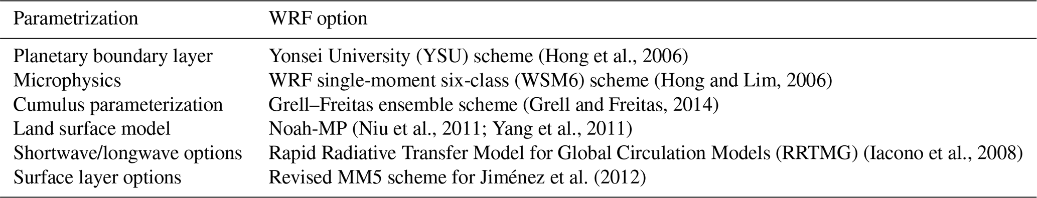
The WRF version 3.8.1 (Skamarock et al., 2008) with the Advanced Research WRF (ARW) dynamical core was used to produce meteorological fields for the CMAQ model simulations. The ARW dynamical core employs fully compressible and nonhydrostatic Euler equations, together with Arakawa C-grid staggering. In the WRF simulations, the final (FNL) operational global analyses data produced by the NCEP (Saha et al., 2010) were used for the ICs and BCs. Temporal and spatial resolutions of the FNL data are 6 h and 0.25^∘, respectively. To minimize the uncertainty in the meteorological fields, the ground measurements and vertical radiosonde data were also assimilated with 3 and 6 h intervals, respectively, with the Newtonian relaxation (or nudging) method (Stauffer and Seaman, 1990). The hourly meteorological fields were provided by the WRF model simulations, and they were then converted into CMAQ-ready format via the Meteorology–Chemistry Interface Processor (MCIP v4.3; Otte and Pleim, 2010). Table 1 summarizes the detailed model configurations of the WRF model simulations.

Table 1 WRF model configurations selected in this study.

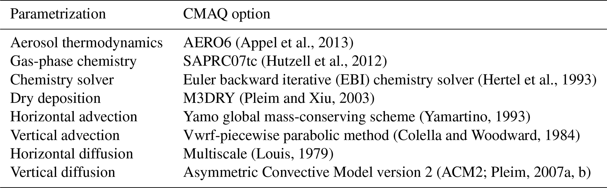
The CMAQ model v5.1 (Byun and Ching, 1999; Byun and Schere, 2006) was used in this study to simulate the atmospheric photochemistries, aerosol dynamics, aerosol thermodynamics, and transport of atmospheric species. The CMAQ runs have two domains in accordance with our experimental purposes. The horizontal resolutions of the mother domain (D1) and daughter domain (D2) are 27 and 9 km, respectively, with 15 vertical layers, while the model top is at 20 km. Table 2 lists the CMAQ model configuration.

Table 2 CMAQ model configurations selected in this study.​​​​​​​

The mother domain (D1) for the CMAQ model simulations covers northeastern Asia including China, the Korean Peninsula, and Japan, and the daughter domain (D2) nested in the D1 targets South Korea (refer to Fig. 1). With this nesting configuration, we intended to examine how the BCs provided by D1 affect the PM_2.5 predictability in D2. Because the PM_2.5 predictability in South Korea is the focus of this study, most of the experiments were carried out in D2, while model simulations over D1 were used to provide D2 with BCs. Table 3 summarizes the domain descriptions for the WRF and CMAQ model runs.

Table 3 Domain descriptions for WRF and CMAQ models.

^* The 15 mid-layer heights correspond to 16, 57, 123, 206, 332, 503, 676, 963, 1468, 2174, 3071, 4119, 5614, 8337, and 13 636 m of altitude above ground level.

For another important input field into the CMAQ model simulations, emission data were prepared. KORUS v2.0 emission fields (Jang et al., 2020) were employed for anthropogenic emissions in the two domains. This emission inventory also supported official CTM simulations for the KORUS–AQ field campaign in 2016. To prepare biogenic emissions, the Model of Emissions of Gases and Aerosols from Nature (MEGAN v2.1; Guenther et al., 2006, 2012) was run with MODIS land cover data (Friedl et al., 2010), together with MODIS-derived leaf area index (LAI) (Myneni et al., 2002; Yuan et al., 2011). For the MEGAN runs, the same meteorological fields generated from the WRF model simulations were used. For the considerations of fire emissions, the Fire Inventory from NCAR (FINN) was used (Wiedinmyer et al., 2006, 2011​​​​​​​).

The observation data used in the EnKF DA experiments were PM_2.5 data obtained from ground stations located in China and South Korea. We acquired the PM_2.5 data over China from the China urban air quality real-time data release platform (http://106.37.208.233:20035​​​​​​​​​​​​​​, last access: 3 March 2020​​​​​​​) managed by the Chinese Ministry of Ecology and Environment, along with another complementary website (http://www.pm25.in, last access: 3 March 2020​​​​​​​). For the PM_2.5 data over South Korea, the data were downloaded from the National Ambient air quality Monitoring Information System (NAMIS) of Korea (https://www.airkorea.or.kr, last access: 3 March 2020). The maximum available observations for PM_2.5 throughout the period of KORUS–AQ campaign were 866 and 165 in China and South Korea, respectively. Figure 1 shows the locations of those ground stations in D1 and D2.

2.4 Experimental setup

For the control run (CTR) without DA, hourly predictions were conducted in D1 by the CMAQ model simulations to generate the BCs for D2. After that, using the BCs we implemented 24 h CMAQ predictions over D2 each day from 25 April to 12 June 2016, with the first 5 d for spin-up and the sixth day for adapting times for the EnKF DA. To provide the meteorological inputs into the CMAQ model runs over D2, the WRF model simulations were initialized each day 12 h before the CMAQ initialization. In this case, the first 12 h simulations were regarded as the spin-up times of the meteorological model. To initialize the next 24 h predictions, the CMAQ model utilized the last hour outputs from the previous 24 h predictions.

The initial ensemble of 40 runs was made based on the CTR output obtained at 00:00 UTC on 30 April by perturbing ICs, as described in Sect. 2.1. The ensemble propagations of the CMAQ model simulations started at 00:00 UTC on 30 April. The DA interval for reanalysis purposes was determined to be 6 h. At the end of the first 6 h prediction (or propagation) of this initial ensemble, the first EnKF DA of PM_2.5 was conducted at 06:00 UTC on 30 April, and the updated initial fields from the EnKF DA are termed the “analysis ensemble” (${\mathit{x}}_{i,k}^{\mathrm{a}}$). These analysis states were again propagated until the next EnKF DA step (12:00 UTC) and were then used as the background state (${\mathit{x}}_{i,k+\mathrm{1}}^{\mathrm{f}}$) in the next DA step (Eq. 3). Following this process, the analysis–prediction cycle was repeated in the DA sequences to correct the ICs using the EnKF method. Note that the last DA was carried out at 18:00 UTC on 11 June, and the first three cycles were considered to be an adapting time for EnKF. Consequently, the analysis–prediction outputs acquired from the four time cycles a day are considered to be a reanalysis run (“ANL”) rather than predictions. Meanwhile, 24 h predictions (i.e., 24 h DA interval) were also carried out every day, starting from 00:00 UTC on 1 May to 11 June, with the mean state of the analysis fields (x^a). A total of 42 d predictions are performed for the prediction run (“PRD”) in this study. Figure S1 of the Supplement shows a schematic of these prediction cycles.

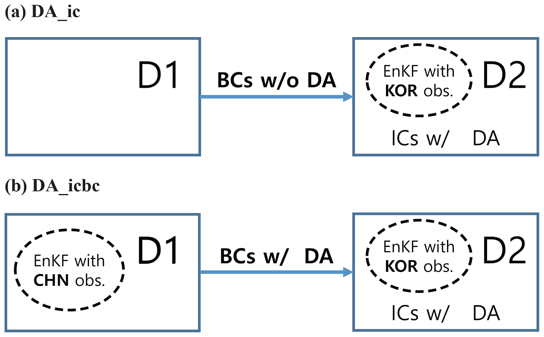
Figure 2 Schematic flowchart for the experiments performed in this study. To evaluate PM_2.5 predictability in South Korea, (a) the DA_ic experiment updates the initial conditions (ICs) only within D2, while (b) the DA_icbc experiment provides D2 with updated boundary conditions (BCs) via assimilating ground observations in China (CHN obs.) and also updating the ICs for D2 using Korean ground observations (KOR obs.).

In addition to the CTR run, the two experiments labeled DA_ic (Fig. 2a) and DA_icbc (Fig. 2b) were also made over South Korea (D2). In both the DA_ic and DA_icbc runs, ground-level PM_2.5 collected in D2 was assimilated to update the ICs. The only difference between the two experiments is the process of acquiring the BCs. In the DA_ic experiment, the BCs were obtained from the CTR run over D1, while in the DA_icbc experiment, the BCs were obtained from the runs with the EnKF DA using ground-measured PM_2.5 collected in China. The technical methods to run the ANL and PRD simulations were the same in both the DA_icbc and DA_ic experiments.

In the DA_ic experiment, we updated only ICs, while in the DA_icbc experiment, we updated both the ICs and the BCs. The goals of this experimental setup are to make it possible to evaluate how much and to what degree the EnKF DA technique could enhance the PM_2.5 prediction skills and to separately estimate the contributions of the improved ICs and BCs to the predictabilities of PM_2.5 over South Korea.

3 Results and discussion

3.1 Impact of the improved initial fields

Figure 3 shows the daily variations of surface PM_2.5 from 1 May to 12 June 2016 (KORUS–AQ period). In Fig. 3, the observations (OBS), denoted by open circles, were obtained by averaging all the ground PM_2.5 available in South Korea (we call this the “aggregation plot”). The simulation results (CTR, ANL with the 3D-Var, and ANL with the EnKF) were also calculated by averaging the model outputs at the corresponding observation locations. Figure 3 shows that the control run (CTR) without DA (solid blue line) tended to consistently underestimate the daily averaged PM_2.5 throughout the simulation period. The ANL simulation with the EnKF (solid red line) showed the best agreement with the observations. The performances of the EnKF are also found to be better than those of the 3D-Var (dashed purple line).

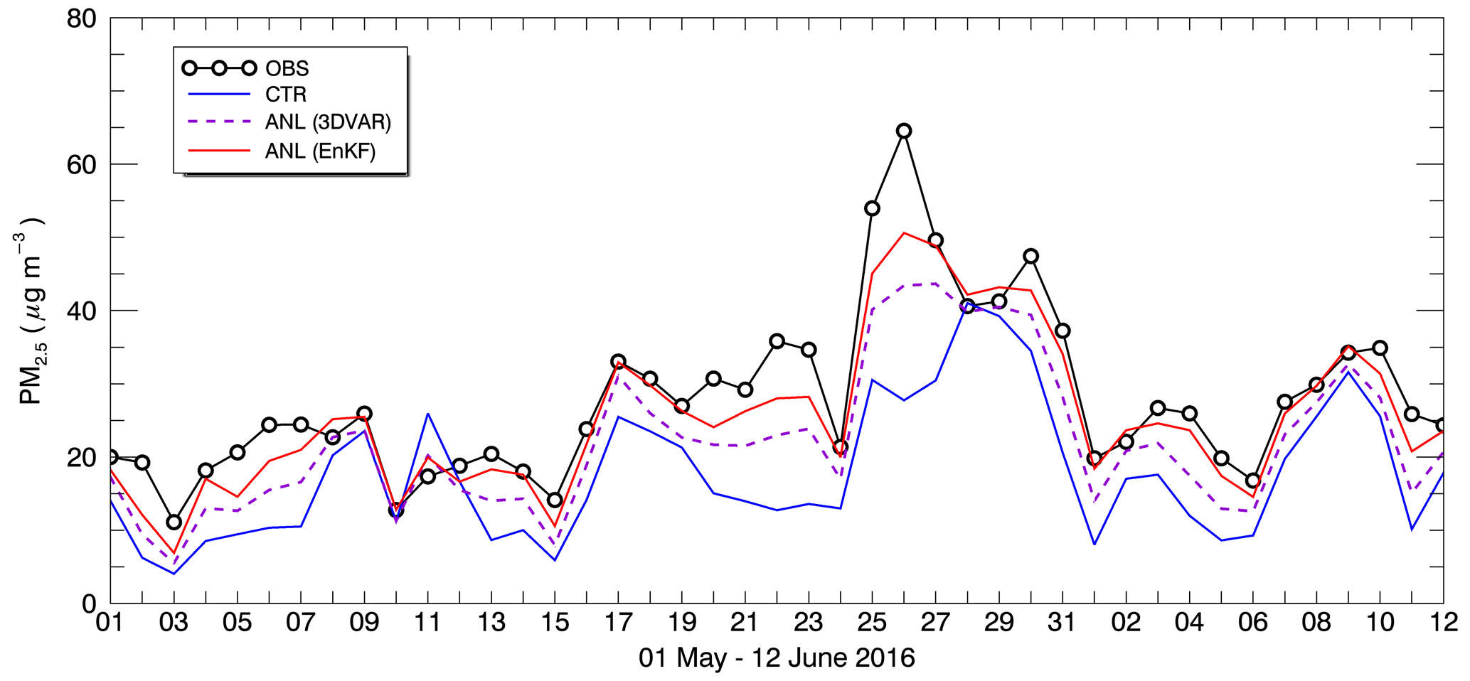
Figure 3 Daily variations of surface PM_2.5 for the DA_ic experiment. Observations (OBS) are represented by a black solid line with open circles. Model results for the control (CTR) run without DA, the reanalysis (ANL) run with 3D-Var, and reanalysis ANL with EnKF are plotted with a blue solid line, purple dashed line, and red solid line, respectively. Values were prepared from daily averages at all the observation sites in South Korea (D2).

Figure 4a and b present the horizontal distributions of surface PM_2.5 for the background and analysis fields at a specific EnKF DA sequence, respectively. Here, the “analysis field” indicates the ICs updated by the EnKF method. Figure 4a and b also plot the observed PM_2.5 used in the DA with the same color scale. Figure 4c gives the analysis increments representing the extent of the corrections of PM_2.5 by the EnKF data assimilation. Again, the background fields tended to underestimate the PM_2.5 over the inland areas. As discussed in Sect. 2.4, Fig. 4b was obtained using an average of 40 analysis ensembles. It can be seen how the estimated background error covariance with a short-term ensemble propagation could correct the model background by assimilating observations. At a relatively isolated ground station, such as Jeju Island (the location is shown in Fig. 1), the analysis increments occurred largely in the downwind area (Fig. 4c). This provides a clear example of flow-dependent correction of the EnKF technique. As another example for clearly showing flow-dependent behavior, the increment comparison between 3D-Var and EnKF is presented in Fig. S2 of the Supplement.

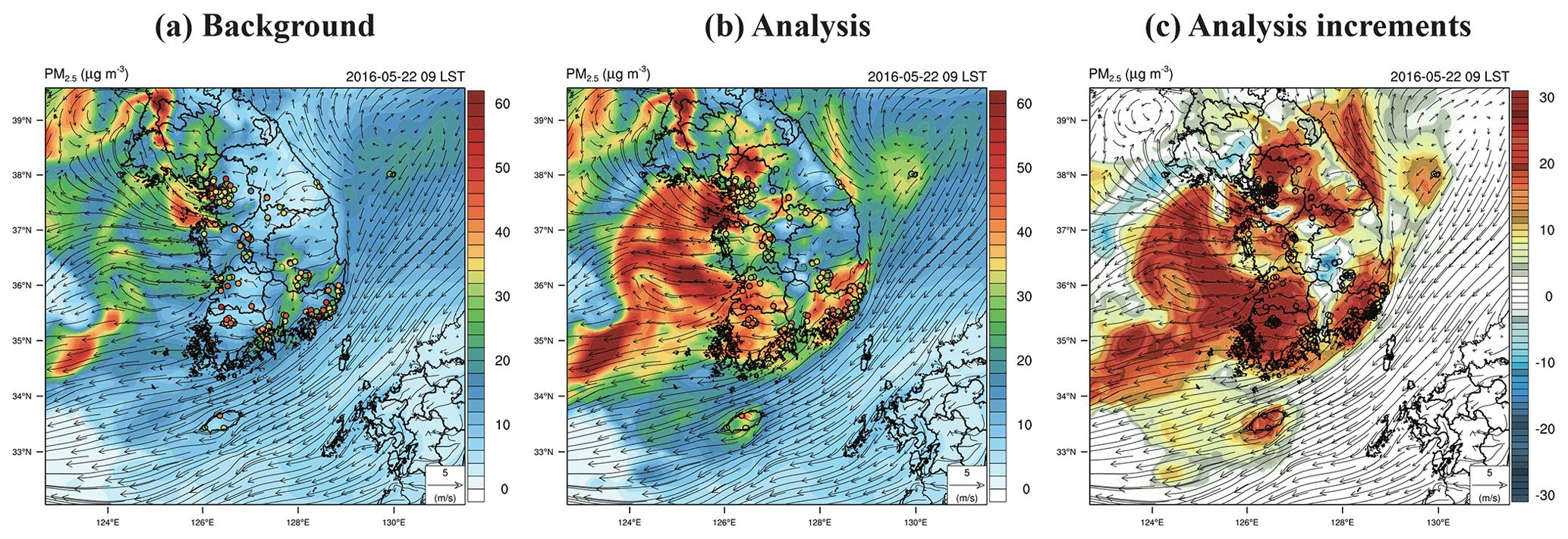
Figure 4 Snapshots of the horizontal distributions of PM_2.5 before (a background) and after (b analysis) the application of the EnKF technique at 00:00 UTC on 22 May 2016. The observed concentrations are also shown on the map with the same color scales as contour values. In the right-hand panel (c), the analysis increments are also presented, and flow-dependent corrections are visible when the wind vectors are overlaid with the analysis increments. The big island in the Southern Sea of the Korean Peninsula is Jeju Island, where the flow-dependent behavior can be noticed.

Figure 5 presents the average diurnal variations generated by aggregating the PM_2.5 data during 42 d from all the observation sites. The vertical bars indicate 1 standard deviation of the averaged samples. Figure 5 shows a clear pattern of the results from each simulation, showing distinct diurnal variations. This pattern appears to be caused mainly by the changes in meteorological fields during the day. During daytime, relatively high mixing height due to the thermal and mechanical development of boundary layers could lead to decreased PM_2.5 within the boundary layers. In contrast, after sunset, PM_2.5 started to increase because the mixing height became shallow due to the stable atmospheric conditions caused by sunset and the weak wind speeds. This diurnal pattern was also found in the observation data, but their variations are weaker than those from the model simulations. The CTR experiment again consistently underestimated the diurnal PM_2.5 throughout a day. However, quite good agreement with the observed PM_2.5 was found in the ANL simulations with the EnKF (solid red line). Focusing on the mean values only at each DA time (00:00, 06:00, 12:00, and 18:00 UTC), the updated concentrations for the 3D-Var simulations (purple triangles) are always closer to the observations than those for the EnKF simulations (red triangles). This indicates that the 3D-Var used larger model errors with higher uncertainties than those of the EnKF when the DA process was carried out. However, the EnKF showed better performance than the 3D-Var simulations in the following time, especially during the daytime (e.g., 01:00 to 06:00 UTC and 07:00 to 12:00 UTC), although its correction strength by assimilation is lower than the 3D-Var. We believe this is because the flow-dependent characteristics of model errors in the EnKF technique improve the model fields more realistically than those in 3D-Var. In contrast, 3D-Var uses a “static” climatological BEC, which usually represents a semi-Gaussian distribution. The better results from the EnKF method (than the 3D-Var method) can also be attributed to the realistic considerations of vertical mixing within the boundary layer in the BEC (Pagowski and Grell, 2012). More sophisticated comparisons in the configurations, such as error variances, observation operator, and vertical length scale of the BEC, are necessary in future study for a direct comparison of the two DA algorithms. To more quantitatively evaluate the performances of the 3D-Var and EnKF techniques, Table 4 also summarizes the statistical metrics based on the reanalysis outputs (ANL). Section 3.4 below discusses the quantitative evaluation in more detail.

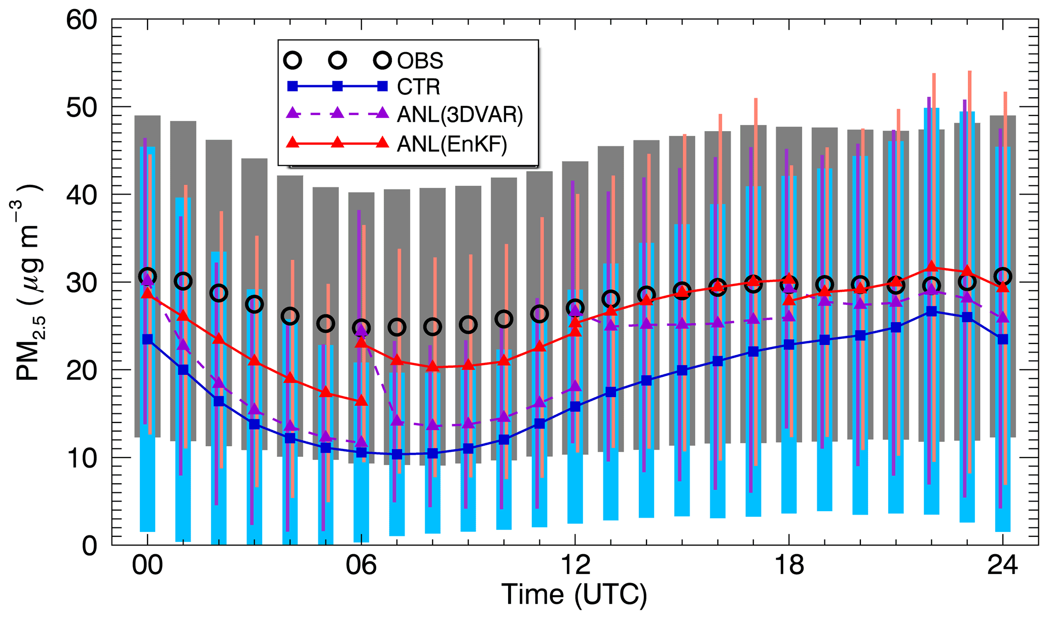
Figure 5 Average diurnal variations of PM_2.5 aggregated from all ground stations in South Korea (D2) for the DA_ic experiment. The color labels are the same as in Fig. 1, except for symbols. The error bars with gray, cyan, purple, and pink indicate 1 standard deviation (±σ) for OBS, CTR, ANL by 3D-Var, and ANL by EnKF simulations, respectively.

Table 4 Statistical metrics for the experiments of DA_ic and DA_icbc. Experiments were evaluated for the 6-hourly assimilated analysis run (ANL) and for the 1 d prediction run (PRD). The ANL run using 3D-Var in the DA_ic experiment is included for comparison.

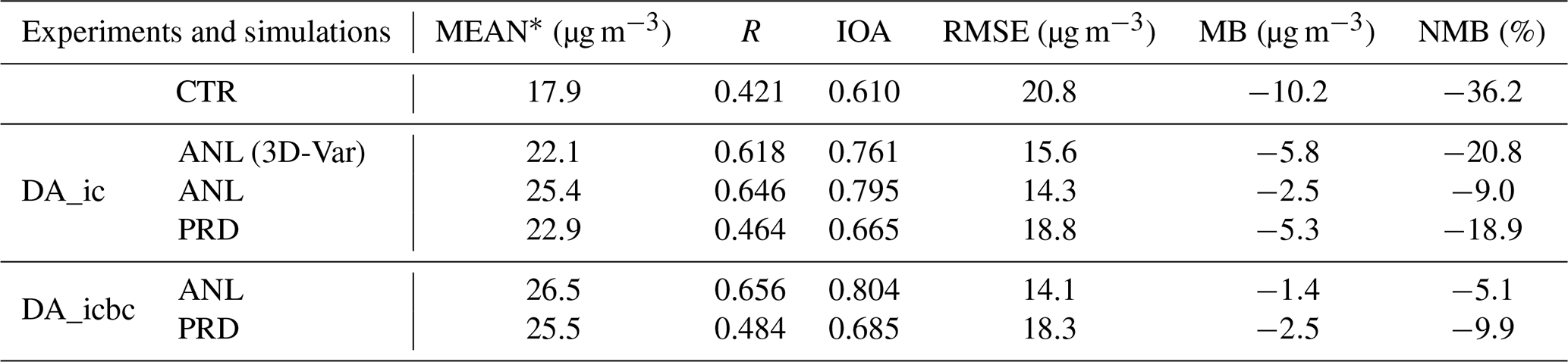
^* Mean concentration in observed data is 27.9 µg m⁻³.

3.2 Impact of the improved boundary conditions

In the previous section, we examined the effects of the initial fields (the DA_ic experiment) in South Korea. The influences of the updated ICs tend to quickly disappear with time over the relatively small domain (D2), particularly when atmospheric flows are fast. In this section, we conducted additional assimilation with the ground observations from China in D1, in addition to the data assimilation with ground observations from South Korea (the DA_icbc experiment). The DA_ic and DA_icbc experimental results were again compared in South Korea, which is our main domain of interest. Although the prediction strategy (refer to Fig. S1 of the Supplement) was the same in the DA_icbc experiment, only PRD runs are shown in this section for simplicity.

Figure 6 shows the averaged PM_2.5 used for the four lateral boundaries of domain 2 in both the DA_ic and DA_icbc experiments. At the four lateral boundaries, PM_2.5 was averaged over 6 weeks, and Fig. S3 of the Supplement shows the south, east, north, and west boundaries of domain 2 (D2). The color-filled contours on the vertical planes correspond to the longitudinal direction from west to east (latitudinal direction from south to north) and the vertical direction for the southern and northern (western and eastern) boundaries of domain 2. Together with the PM_2.5, Fig. 6 also plots the mean wind velocity across the four boundaries to show the inflow into D2 and outflow from D2 with positive (solid) and negative (dashed) contour lines, respectively. In the upper panels of Fig. 6, the western part of the north boundary and northern part of the west boundary show relatively high PM_2.5 (>15 µg m⁻³) within 1 km of altitude. Although long-range transport of air pollutants from China to South Korea sometimes occurs in the upper layers, the averaged PM_2.5 at the northwest boundaries were high within the boundary layer. We should also note in Fig. 6 that the northwestern boundary had a strong inflow that could result in high PM_2.5 in D2.

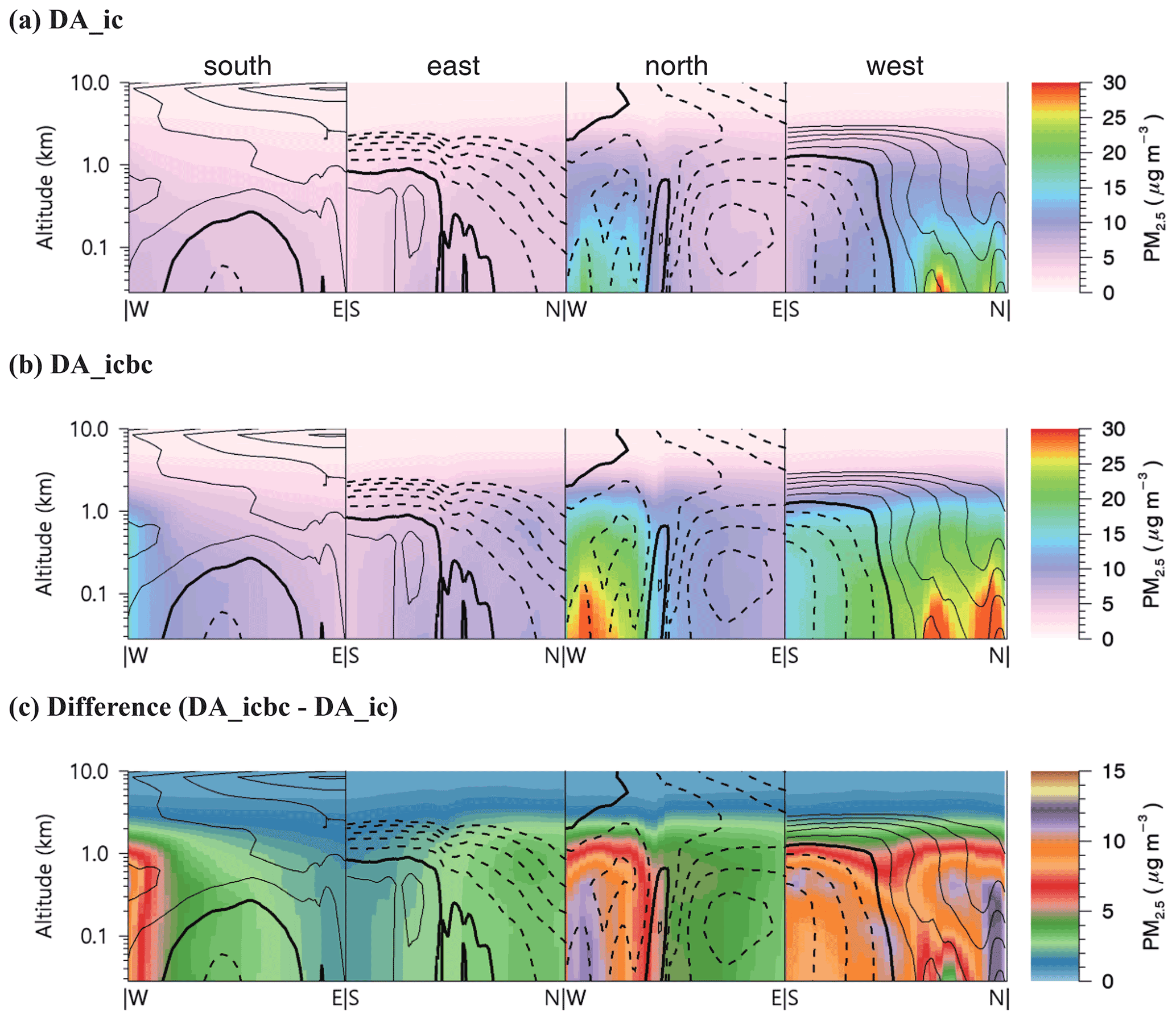
Figure 6 Averaged PM_2.5 distributions in the four lateral boundaries of the domain 2 (D2: south, east, north, and west from the left to the right, refer to Fig. S4 of the Supplement). Each panel includes black contour lines that explain the inflow (solid lines) and outflow (dashed lines) wind vector with 1 m s⁻¹ intervals. The thick black lines indicate zero wind speed. In (a) DA_ic and (b) DA_icbc, the averaged lateral boundary conditions are provided into D2 without and with the EnKF data assimilation in China (D1), respectively. The increments in DA_icbc experiment are also presented in the bottom panel (c). Note that the y axis for altitude is presented in log scale to emphasize the results below the boundary layer.

The middle and bottom panels of Fig. 6 show that at all the boundaries, the DA_icbc experiment exhibited higher PM_2.5 than the DA_ic experiment. This indicates that the control simulation without assimilation (CTR) over D1 under-calculated PM_2.5 in China. Figure 6c shows that there are small changes in PM_2.5 above 2 km of altitude, while the changes become larger within the boundary layers. To quantify the amounts transported into and out of D2, we calculated the PM_2.5 fluxes by multiplying PM_2.5 by wind velocities and then averaged them over the simulation period (refer to Fig. S4 of the Supplement). The cross-sectionally averaged PM_2.5 flux at the west boundary increased from 19.2 to 26.6 µg m⁻² s⁻¹ from the DA_ic to DA_icbc experiments. This indicates that larger amounts of PM_2.5 were actually transported long distances from China to South Korea, mainly through the northwestern boundary of domain 2 during the KORUS–AQ period.

A ground station where the influence of the BCs can be checked is Baekryeong-do, South Korea (shown with a star symbol in Fig. 1). This is because Baekryeong-do is located at the west end of domain 2 (nearby the western boundary of D2) and is also minimally affected by local inland emissions (i.e., there are no major industries and only a small population living on the island). Figure 7a shows the averaged diurnal variations of PM_2.5 at Baekryeong-do evaluated from D1. Hence, the results with (solid red line with triangles) and without (blue dashed line with rectangles) the DA can be perceived as the BCs in D2 for the DA_icbc and DA_ic experiments (refer to Fig. 2), respectively. The averaged diurnal variation of PM_2.5 without the DA is in the range between 10 and 20 µg m⁻³, which is approximately 10 µg m⁻³ lower than the observed PM_2.5. However, when the assimilation of the observations in China was applied, almost the same levels of PM_2.5 as the observations were reproduced. We found that the 24 h predictions that were evaluated at the same location in D2 were greatly improved (Fig. 7b). This is confirmed by the results from the DA_icbc experiment in Fig. 7b. Since the observed PM_2.5 at the Baekryeong-do site was assimilated to improve the ICs in both the DA_ic and DA_icbc experiments, the predictions started from a similar PM_2.5 as the observed PM_2.5. However, the predictions for the DA_icbc experiment agreed greatly with the observed PM_2.5 owing to the application of accurate BCs, while the prediction for the DA_ic experiment rapidly converged to the CTR run because of the same BCs as the CTR run. It should also be noted that analysis increments by assimilating Baekryeong-do data for the DA_icbc experiment in D2 would be minimal, as the background PM_2.5 was already close to the observed PM_2.5 because of the updated BCs.

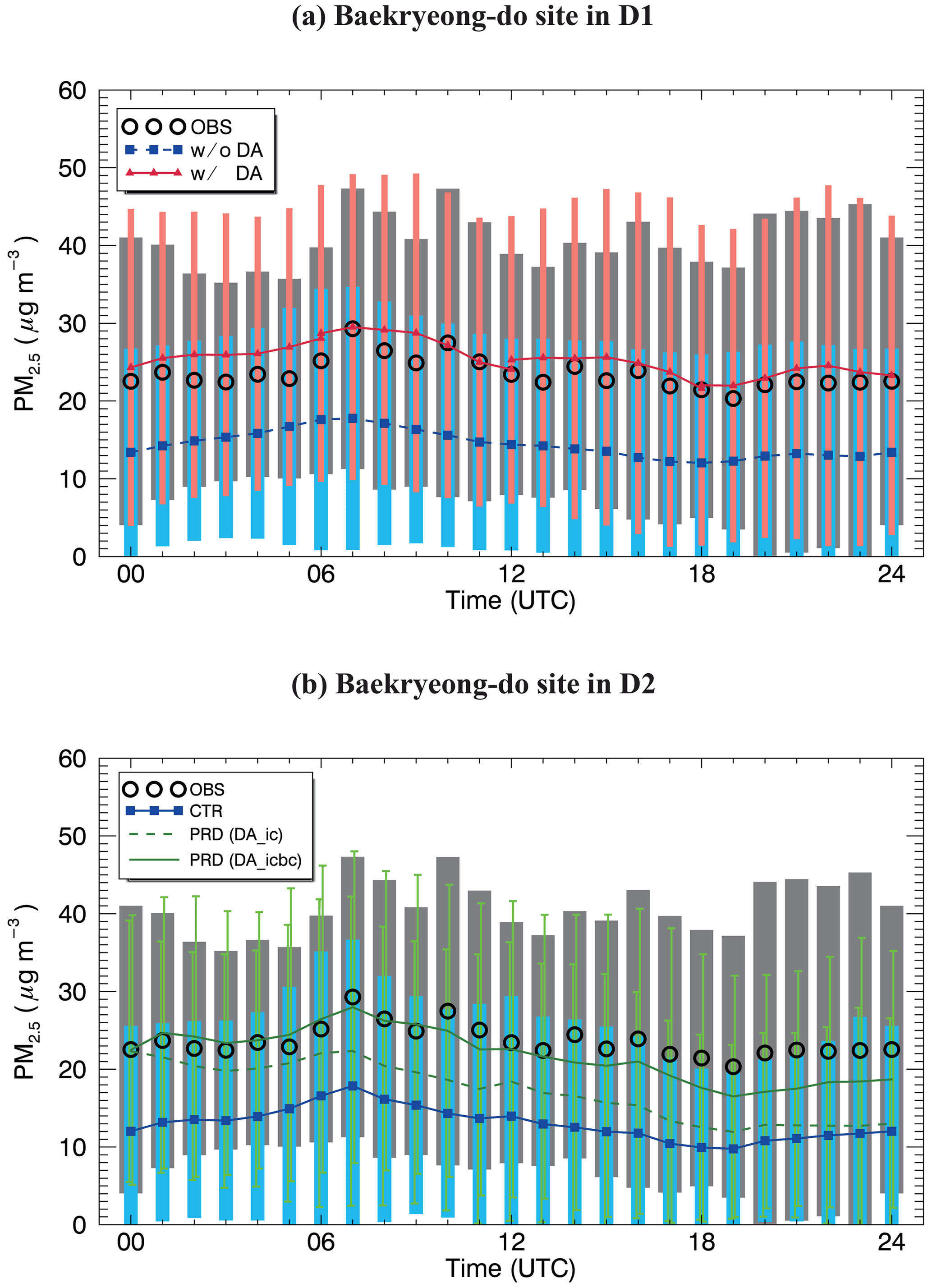
Figure 7 Averaged diurnal variations of PM_2.5 aggregated at the Baekryeong-do site from the results obtained in (a) D1 and (b) D2. The line colors and symbols are the same as in Fig. 5, except for the prediction runs in D2, which are plotted by dashed and solid green lines for the DA_ic and DA_icbc experiments, respectively, in panel (b).

Figure 8 presents the daily variations of PM_2.5 like in Fig. 3, except for the results from the “PRD runs” for the DA_ic and DA_icbc experiments. The PRD runs are technically the same as the ANL runs except for the prediction lead time (of 24 and 6 h, respectively). Again, significant improvements in the DA_ic and DA_icbc experiments were found compared to the results from the CTR run. When the dominant synoptic wind directions were southerly or easterly (e.g., on 2 to 4 June), there were only small differences between the DA_icbc and DA_ic experiment, and thus limited improvements were achieved. Similarly, no improvements for updating the boundary condition in the DA_icbc experiment were found during the precipitation days on 10 and 24 May and on 1 and 6 June. However, large improvements could be made when the yellow dust event occurred from 4 to 7 May and when the westerly winds prevailed over D2 between 20 and 27 May (except on 24 May). An example of the impact of the updated BCs for the DA_icbc experiment is shown in Fig. S5 of the Supplement, which explains the higher transboundary PM_2.5 after assimilating ground PM_2.5 observations in China. Therefore, to improve the predictability of PM_2.5 in South Korea, it is of great importance to provide appropriate BCs by assimilating the ground observation data in the upwind area (i.e., EC, NC, and NEC region, refer to Fig. 1).

Figure 8 Daily averaged variations of PM_2.5. The lines and colors are the same as in Fig. 3, except for the 1 d prediction runs (PRD). The 1 d predictions only with updated initial conditions (DA_ic) and with initial and boundary conditions (DA_icbc) are presented by the dashed and solid green lines, respectively.

To evaluate the PM_2.5 predictability in South Korea, Fig. 9 also displays the averaged diurnal variations and compares the prediction runs (PRD) for the two experiments, DA_ic and DA_icbc. The performances of 24 h predictions were launched every 00:00 UTC. The predicted PM_2.5 for the PRD runs shows better performances than the CTR run with reduced errors and biases, although the biases are larger than those for the ANL runs (shown in Fig. 3). Again, the averaged diurnal PM_2.5 for the DA_icbc experiment is closer to the observations than that for the DA_ic experiment. This is because the enhanced boundary information was repeatedly provided at the everyday prediction sequence. Also, the negative biases found in the DA_ic experiment were greatly alleviated with the DA_icbc experiment, even if the same emissions and meteorological fields were applied for the 24 h predictions. Immediate improvements could be seen after the predictions started at 00:00 UTC. As time progressed, the biases and errors were also propagated. However, the biases in the DA_icbc experiment became about half of those in the DA_ic experiment. Also note that the slightly overpredicted PM_2.5 for the DA_icbc experiment between 18:00 and 23:00 UTC was caused by insufficient information about vertical mixing during nighttime. Simulated nocturnal boundary layer heights were lower than real boundary layer heights. This is a critical problem in meteorological modeling and has been discussed in many previous publications (Eder et al., 2006; Hong, 2010).

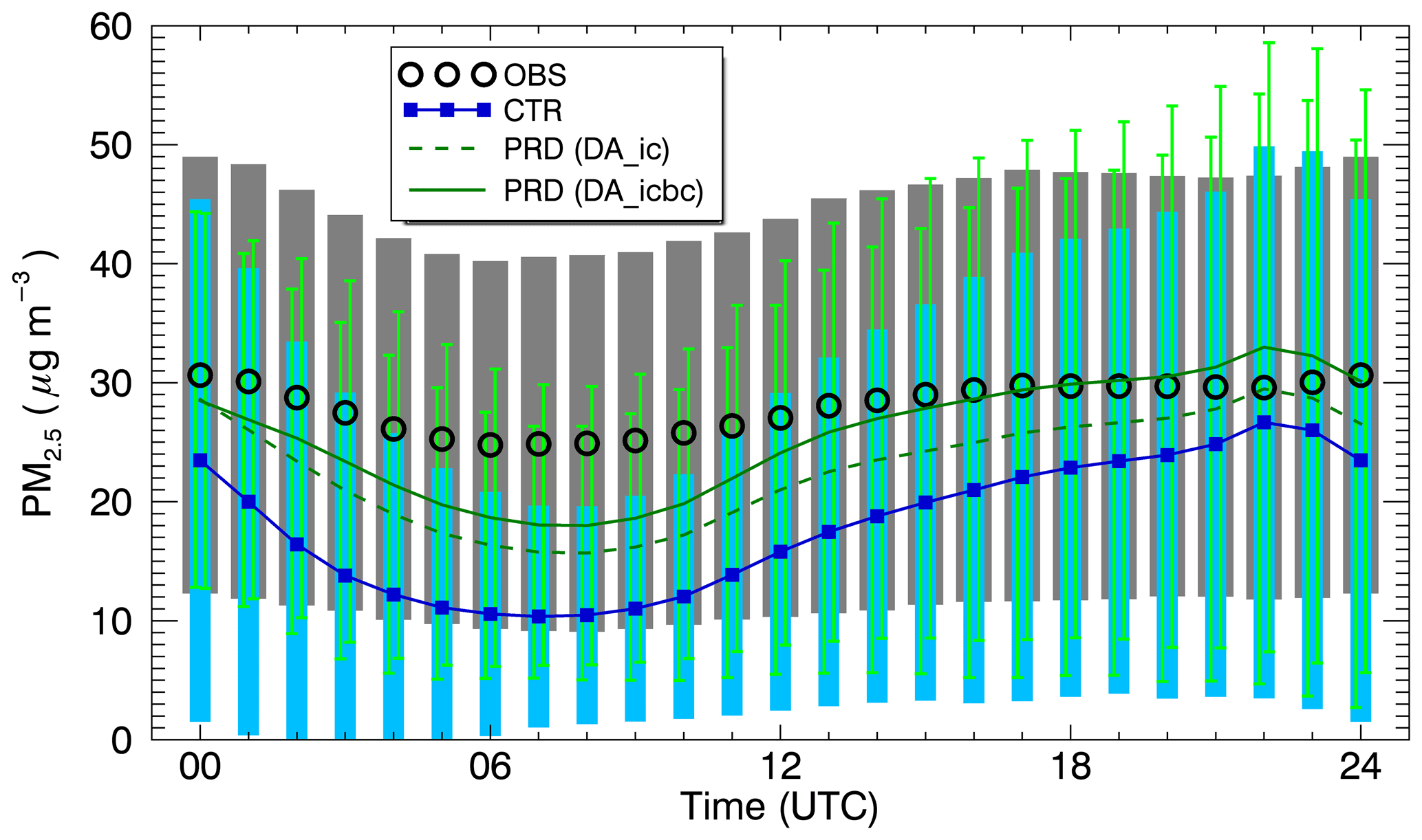
Figure 9 Averaged diurnal variations of PM_2.5 aggregated from all ground stations in South Korea (D2). The color and symbols are the same for observations (OBS) and the control run (CTR) as in Fig. 5. The 1 d predictions only with updated initial conditions (DA_ic) and with initial and boundary conditions (DA_icbc) are presented by dashed and solid green lines, respectively. 1 standard deviation (σ) is also plotted for each case using vertical bars. The left and right vertical bars indicate ±σ for DA_ic and DA_icbc, respectively.

3.3 Statistical evaluations: quantification of contributions by updating the initial and boundary conditions

Table 4 summarizes the statistical performance metrics that were calculated to evaluate the model performance. Table S1 of the Supplement provides the mathematical definitions for the performance metrics. Because the evaluations were conducted using hourly data, including the prediction hours, we did not consider a spatially independent observation. Moreover, it is difficult to randomly select sparse observation sites (D2 in Fig. 2). Therefore, the statistical metrics were calculated including the same observation data as those used in DA and were compared under the same conditions for all the experiments. The average PM_2.5 over the entire simulation period was 27.9 µg m⁻³, and the CTR run produced an underestimated PM_2.5 of 17.9 µg m⁻³. The application of the updated ICs (the DA_ic experiment) improved the average PM_2.5, which was 25.4 and 22.9 µg m⁻³ for the ANL and PRD runs, respectively. The results for the DA_icbc experiment were even closer to the observations than those of the DA_ic. The average PM_2.5 from the ANL and PRD runs for the DA_icbc experiment was 26.5 and 25.5 µg m⁻³, respectively. All the statistical metrics for the DA_icbc experiment were improved compared to the DA_ic experiment. Focusing on the PRD runs, the IOA increased significantly from 0.610 to 0.665 (for the DA_ic experiment) and then to 0.685 (for the DA_icbc experiment). The root mean square error (RMSE) was reduced from 20.8 to 18.3 µg m⁻³ for the DA_icbc experiment, while it was 18.8 µg m⁻³ for the DA_ic experiment. This small reduction in the averaged RMSE between the DA_ic and the DA_icbc experiments can be attributed to the overprediction of PM_2.5 during the nighttime, as Fig. 9 shows. On the other hand, remarkable improvements were found in the MBs. In the DA_ic experiment, the averaged MB was drastically reduced from −10.2 to −5.3 µg m⁻³. Another large reduction in the averaged MB was found from −5.3 to −2.5 µg m⁻³ from the DA_ic experiment to the DA_icbc experiment. The normalized MB (NMB) was also reduced by 17.3 % in the DA_ic experiment from 36.2 % for the CTR run. In addition, the DA_icbc experiment led to another considerable decrease in the NMB by 9.0 % compared to the DA_ic experiment.

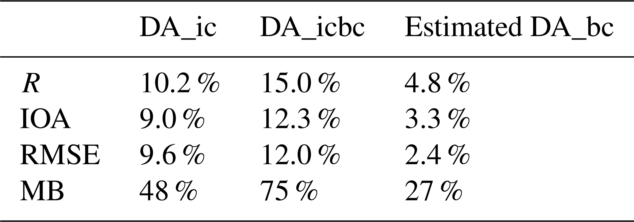
To investigate the quantitative contributions of the ICs and BCs to the model performance, we calculated the “rate of improvement (ROI)” with respect to the PRD results (see Table 5). The ROIs are defined by the ratios of enhanced (R​​​​​​​ and IOA) or reduced (RMSE and MB) corresponding statistical metrics to those calculated from the CTR run. Based on the ROI for the DA_ic and DA_icbc experiments, we can estimate the ROIs associated with the initial correction (the DA_ic) and the boundary correction (the DA_bc). The ROIs for the DA_ic and DA_icbc experiments were 10.2 % and 15.0 % in terms of R​​​​​​​ (Pearson's correlation coefficient), respectively. Therefore, the estimated ROI due to the DA_bc might be 4.8 %. The contributions in MB can also be estimated quantitatively in terms of the ROIs. Updated BCs resulted in an improvement of 27 % in the MB in terms of ROI. In the case of the applications of the DA_ic and the DA_bc, the ROIs showed a 9.0 and 3.3 % increase in terms of IOA and a 9.6 % and 2.4 % decrease in terms of RMSE, respectively.

Table 5 Rate of improvement (ROI) by EnKF data assimilation in 1 d predictions. The ROI is the ratio of the enhanced (R​​​​​​​ and IOA) or reduced (RMSE and MB) statistical metrics to those for the CTR simulation. The ROI by updating boundary conditions (DA_bc) can be estimated from the difference between that obtained by the DA_ic and DA_icbc experiments.

4 Conclusions

To improve PM_2.5 prediction in South Korea, we developed and applied an EnKF data assimilation method to the WRF–CMAQ modeling system. For data assimilation, we employed two groups of ground observations from China and South Korea. We found that when we updated the ICs via the EnKF data assimilation, the PM_2.5 predictions in South Korea could be greatly improved. In a comparative analysis between EnKF and 3D-Var, the EnKF technique showed better performance than 3D-Var in short-term PM_2.5 predictions. These results indicate that the BEC used in this study can realistically reflect the current state of the atmosphere, particularly in the boundary layer.

This study also highlighted the importance of updating BCs to further enhance the PM_2.5 predictability over South Korea. Long-range transport from China directly impacts the air quality in South Korea, particularly during high-PM_2.5 episodes. Because effects to implement DA with ground observations inside South Korea are restrictive in terms of improvement in analysis fields and predictions, we updated the inflow BCs via the EnKF DA that uses observations in China. A comparison of the studies with and without the updated BCs suggested that improved ICs (the DA_ic experiment) reduced the NMBs from −36.2 to −18.9 % compared to the control run, and even further updating the ICs and BCs (the DA_icbc experiment) improved the NMBs from −36.2 to −9.9 % in terms of the 24 h PM_2.5 prediction over South Korea. In terms of IOA (in terms of MB), the contributions of updating the ICs and BCs to 24 h predictability were estimated to be 73 and 27 % (63 and 37 %), respectively. However, caution should be exercised in that these estimations are made only for a specific period (KORUS–AQ campaign) and can vary with atmospheric conditions. A longer test period is needed for general quantification.

Recently, the EnKF has also been used to assimilate satellite-retrieved aerosol observations (e.g., Sekiyama et al., 2010; and Yin et al., 2016). Other groups also used the EnKF method for the joint optimization of ICs and emission scaling factors (e.g., Tang et al., 2011; Peng et al., 2017 and 2018). As we have shown that the consideration of transboundary air pollution is of significance in the PM_2.5 predictions over South Korea, assimilating aerosol optical depth (AOD) data from satellites over the Yellow Sea (where no ground observations are available) is expected to provide the PM_2.5 prediction system with important information.

Throughout this study, the DA method of “perturbed observation EnKF” (first proposed by Evensen, 2003) was employed. However, there are some popular variants of the EnKF method that obviate the need to perturb observations, such as the ensemble square root filter (EnSRF; Whitaker and Hamill, 2002), ensemble adjustment Kalman filter (EAKF; Anderson, 2001), and local ensemble transform Kalman filter (LETKF; Hunt et al., 2007). Two of these EnKF variants are also being tested to alleviate the sampling errors in the observation ensemble, and the results will also be reported in the near future in the context of further development of the ensemble data assimilations and the Korean air quality prediction system.