Constraining a land cover map with satellite-based aboveground biomass estimates over Africa

Most land surface models can, depending on the simulation experiment, calculate the vegetation distribution and dynamics internally by making use of biogeographical principles or use vegetation maps to prescribe spatial and temporal changes in vegetation distribution. Irrespective of whether vegetation dynamics are simulated or prescribed, it is not practical to represent vegetation across the globe at the species level because of its daunting diversity. This issue can be circumvented by making use of 5 to 20 plant functional types (PFTs) by assuming that all species within a single functional type show identical land–atmosphere interactions irrespective of their geographical location. In this study, we hypothesize that remote-sensing-based assessments of aboveground biomass can be used to constrain the process in which real-world vegetation is discretized in PFT maps. Remotely sensed biomass estimates for Africa were used in a Bayesian framework to estimate the probability density distributions of woody, herbaceous and bare soil fractions for the 15 land cover classes, according to the United Nations Land Cover Classification System (UN-LCCS) typology, present in Africa. Subsequently, the 2.5th and 97.5th percentiles of the probability density distributions were used to create 2.5 % and 97.5 % credible interval PFT maps. Finally, the original and constrained PFT maps were used to drive biomass and albedo simulations with the Organising Carbon and Hydrology In Dynamic Ecosystems (ORCHIDEE) model. This study demonstrates that remotely sensed biomass data can be used to better constrain the share of dense forest PFTs but that additional information on bare soil fraction is required to constrain the share of herbaceous PFTs. Even though considerable uncertainties remain, using remotely sensed biomass data enhances the objectivity and reproducibility of the process by reducing the dependency on expert knowledge and allows assessing and reporting the credible interval of the PFT maps which could be used to benchmark future developments.

1 Introduction

Degradation, fires and deforestation of tropical forests are responsible for two-thirds of the global net deforestation emissions (Houghton et al., 2012; Le Quéré et al., 2015; Friedlingstein et al., 2020). Although African tropical rainforests represent only one third of the global tropical rainforests (Lewis et al., 2009), they were responsible for almost all, i.e., 1.48 Pg C in 2015 and 1.65 Pg C in 2016, of the net carbon (C) emissions of pan-tropical regions, but substantial uncertainty is associated with these estimates, i.e., 1.15 for 2015 and 1.0 Pg C for 2016, mainly driven by fire and land use changes (Palmer et al., 2019). The uncertainty of model estimates, such as mentioned above, broadly comes from three sources: (1) the vegetation distribution in the model, (2) the ability of the model to simulate biomass accumulation of undisturbed vegetation and (3) the ability of the model to simulate natural and anthropogenic disturbances of the standing biomass. As this study will focus on improving the description of the vegetation distribution, the first question that needs to be answered is why vegetation distribution remains so uncertain.

Most land surface models can either calculate the vegetation distribution internally by making use of biogeographical principles (Sitch et al., 2003; Krinner et al., 2005; Clark et al., 2011) or use vegetation maps to prescribe spatial and temporal changes in vegetation distribution. Where the first approach results in a description of the potential vegetation, the second approach is more suitable when actual vegetation is to be studied. Irrespective of whether potential or actual vegetation is studied, it is not practical to represent vegetation across the globe at the species level because there are already over 60 000 tree species (Beech et al., 2017), not to mention the diversity in herbs, forbs and mosses. Land surface models represent this daunting diversity by making use of 5 to 20 plant functional types (PFTs) (Huete et al., 2016). The underlying assumption of plant functional types is that all species within a single functional type show identical land–atmosphere interactions irrespective of their geographical location (Huete et al., 2016; Bonan et al., 2002; Brovkin et al., 1997; Chapin et al., 1996). Discretizing real-world vegetation in PFTs is a first source of uncertainty.

When actual vegetation is the focus of a modeling study, the vegetation distribution will have to be prescribed. The construction of vegetation maps first requires real-world observations, typically through satellite-based remote sensing. Current remote sensing technology does not enable distinguishing individual tree species; hence, vegetation is observed as land cover types (Defourny, 2019) which group vegetation with similar sensory characteristics. The remote sensing observations themselves as well as classifying them in land cover types are the second and third source of uncertainties (Hansen et al., 2013; Mitchard et al., 2014; Hurtt et al., 2004). Because the land surface models require the vegetation to be discretized in PFTs, which may differ between different land surface models, the land cover types will have to be remapped on PFT maps. The rules applied in remapping satellite-based land cover types in PFT maps are formalized in so-called “cross-walking tables” (CWTs) (Poulter et al., 2011, 2015) which are a fourth source of uncertainty (Hartley et al., 2017).

Although CWTs have been extensively used to create PFT maps (Li et al., 2018, 2016; Poulter et al., 2011; Krinner et al., 2005), the process of associating land cover types with specific PFTs remains difficult to reproduce since several iterations of expert knowledge are required (Poulter et al., 2011, 2015). Various land cover classifications exist, including the commonly used FAO (Food and Agriculture Organization) Land Cover Classification System (LCCS; Di Gregorio and Jansen, 2000). Most classes of the LCCS correspond to a mix of PFTs, whose fractions are difficult to assess and likely variable across regions. For example, several classes are labeled as a mosaic of vegetation types (i.e., “mosaic of natural vegetation (tree, shrubs, herbs)”; see Table 2 in Poulter et al., 2015). Not surprisingly, efforts have been made to decrease the need for expert knowledge in favor of more objective and reproducible approaches, e.g., classification rules based on a suite of improved and standard MODIS products (Sun et al., 2008). Moreover, producing PFT maps from satellite-based land cover maps needs to become fully automated when the temporal frequency of satellite-based land cover and biomass maps will increase thanks to the recent Global Ecosystem Dynamics Investigation (GEDI) lidar data (Dubayah et al., 2020) or future synthetic aperture radar (SAR) missions like the NASA-ISRO synthetic aperture radar (NiSAR) or BIOMASS missions (Le Toan et al., 2011; Quegan et al., 2019).

In this study, we hypothesize that remote sensing-based assessments of aboveground biomass (AGB) can decrease the dependency on expert knowledge when setting up CWTs and as such contribute to the automation of the land cover class mapping into PFTs for land surface models. The main rationale is that the aboveground biomass content of an ecosystem provides information on the fraction of tree PFTs of that ecosystem. In this context, the objective of this study are to (1) construct a framework of data assimilation in which biomass remote sensing products can be routinely used to update an existing or create a new CWT, (2) constrain a cross-walking table used to convert the ESA-CCI Global Land Cover map into a PFT map and (3) propagate the credible interval from using a CWT in the production of PFT maps to the simulation results of biomass and albedo maps derived from a land surface model. Such a framework will be applied and tested over Africa using the aboveground biomass product derived by Bouvet et al. (2018) for that continent with the Organising Carbon and Hydrology In Dynamic Ecosystems (ORCHIDEE) land surface model (Krinner et al., 2005), more specifically tag 2.0 revision 6592 close tag 2.2, used for the recent Climate Modeling Intercomparison Project – phase 6 (CMIP6) (Boucher et al., 2020).

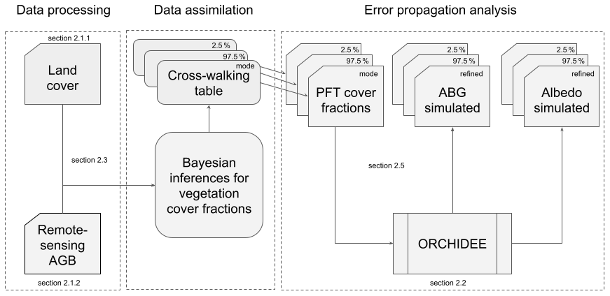
Figure 1 Approach to assimilate the information held by aboveground biomass (AGB) maps into PFT maps. Remote sensing AGB and land cover products are jointly assimilated to obtain cross-walking tables that can be used to make PFT maps. Due to the uncertainty analysis in the data assimilation approach, an ensemble of cross-walking tables and PFT cover fraction maps can be produced. Subsequently, the land surface model ORCHIDEE can be run for different PFT maps to quantify the uncertainty from propagation of the uncertainty from remote sensing products into a model simulation.

2 Materials and methods

2.1 Overview

CWTs (Poulter et al., 2015) are used to convert the 43 land cover types distinguished on the ESA-CCI land cover product into generic plant functional types (13 PFTs in Poulter et al. (2015) distinguished by large-scale land surface models such as the ORCHIDEE model (Krinner et al., 2005) used in this study. These generic PFTs are further grouped and/or divided to match each model-specific PFT classification, using additional grid-cell information to separate grassland and crop C₃ versus C₄ photosynthetic pathway (Still et al., 2003) and to split generic PFTs according to bioclimatic zones (i.e., Koppen–Geiger climate classification map) (see more details for the ORCHIDEE model in Lurton et al., 2020). In this study, we provide a proof of concept by creating a new ORCHIDEE PFT map by combining information from the ESA-CCI land cover product and the AGB product for Africa (Bouvet et al., 2018) to estimate woody, herbaceous and bare soil cover fractions within each land cover type of the ESA-CCI product. Subsequently, the estimated cover fractions are used to constrain the existing CWT and create a new ORCHIDEE PFT map applicable primarily for Africa (Fig. 1). Finally, the impact of using AGB maps to constrain the PFT maps on the skill of the ORCHIDEE model to simulate the contemporary biomass and its spatial distribution over Africa is quantified. Note that the approach is tested over Africa but is generic enough to be applied everywhere.

2.2 Dataset products

2.2.1 Land cover map

ESA's Climate Change Initiative for Land Cover (CCI-LC) produced consistent global LC maps at 300 m spatial resolution on an annual basis for the year 2015 (Defourny, 2019). Only one year (2015) has been used to estimate the new vegetation cover cross-walking table. The typology of CCI-LC maps follows the LCCS developed by the United Nations (UN) FAO to enhance compatibility with similar products such as GLC2000 and GlobCover 2005 and 2009. The UN-LCCS typology was designed as a hierarchical classification, which allows adjusting the thematic detail of the legend. The “level 1” legend, also called “global” legend, counts 22 classes and is globally consistent and thus suitable for global applications such as creating PFT maps for land surface models. The “level 2” or “regional” legend counts 43 classes which are not present all over the world and could be used in this study given its focus on a single continent, i.e., Africa (see Sect. 2.2.3). In addition, the UN-LCCS partly overlaps with the PFTs used in climate models.

2.2.2 Aboveground biomass map

This study also makes use of a continental map of AGB of African savannas and woodlands for the year 2010 (Bouvet et al., 2018). The map has a 25 m resolution and is built from the 2010 L-band data of the Phased Array L-band Synthetic Aperture Radar (PALSAR) on the Advanced Land Observing Satellite (ALOS, 2022) satellite. Covering the African continent required about 180 data strips of which 91 % were acquired between May and November 2010. The remaining 9 % of the domain was filled with imagery from 2009 and 2008. The data have been processed by the Japan Aerospace Exploration Agency (JAXA, Japan Aerospace Exploration Agency, 2022) using the large-scale mosaicking algorithm described in Shimada and Ohtaki (2010), including orthorectification, slope correction and radiometric calibration between neighboring strips and multi-image filtering described in Bouvet et al., 2018.

The continental AGB map was derived as follows: (1) stratification into wet and dry season areas in order to account for seasonal effects in the relationship between PALSAR backscatter and AGB, (2) the development of a statistical model relating the PALSAR backscatter to observed AGB, (3) Bayesian inversion of the direct model to obtain AGB and its credible interval for pixels where no observations are available and (4) masking out non-vegetated areas using the ESA-CCI Land Cover dataset (but see Sect. 2.1.1). The resulting AGB map was visually compared with existing AGB maps (Saatchi et al., 2011; Baccini et al., 2012; Avitabile et al., 2016) and cross validated with AGB estimates obtained from field measurements and lidar datasets (Naidoo et al., 2015). Cross validation revealed a good accuracy of the dataset, with an RMSD between 8 and 17 t ha⁻¹. For more details on the creation and evaluation of the AGB maps, see Bouvet et al. (2018).

2.2.3 Pre-processing

One known limitation of the original AGB map (Bouvet et al., 2018) is the signal saturation and in some cases the decrease of the signal (Mermoz et al., 2015) occurring in L-band SAR for AGB values higher than 85 t ha⁻¹. In order to overcome this issue, a second AGB map was created based on two other ancillary datasets: a map of tree cover (Hansen et al., 2013) and a map of tree height (Simard et al., 2011). The AGB was estimated by deriving an empirical relationship between biomass, available from airborne lidar estimates, and the product of tree cover and tree height. The second version targets dense forest areas such as in the Congo Basin and is used to adjust the AGB values at locations where signal saturation occurred. Because of a coarser resolution from the tree height map (0.01^∘ × 0.01^∘, 100 ha) than the original AGB map (0.00025^∘ × 0.00025^∘, 0.0625 ha), the new biomass map has been rescaled to 0.01^∘ resolution. The rescaling drastically reduced the noise produced by PALSAR measurement artifacts (Thuy Le Toan, personal communication, 2020). The original AGB map was downscaled by an average resampling method, i.e., computing the weighted average of all contributing pixels. To do so, we used the Gdalwarp function from GDAL (GDAL/OGR contributors, 2022). The map used in this study is a composite of the two versions of the biomass map by using the following rules:

• For broadleaved evergreen forests (UN-LCCS land cover type 50), flood forests (UN-LCCS 160) and closed broadleaved deciduous forests (UN-LCCS 61), the map based on tree cover and tree height was used because there are no AGB estimates in the map based on PALSAR.

• For broadleaved deciduous forests (UN-LCCS 60), the maximum between the two maps was used because its biomass ranged around the threshold of 85 t ha⁻¹ and may create truncated distribution.

• For the other land cover types, which typically have a biomass well below 85 t ha⁻¹, the AGB value from the PALSAR map was used because it is considered more reliable than the statistical relationship between biomass, vegetation cover and vegetation height especially for the lower biomass.

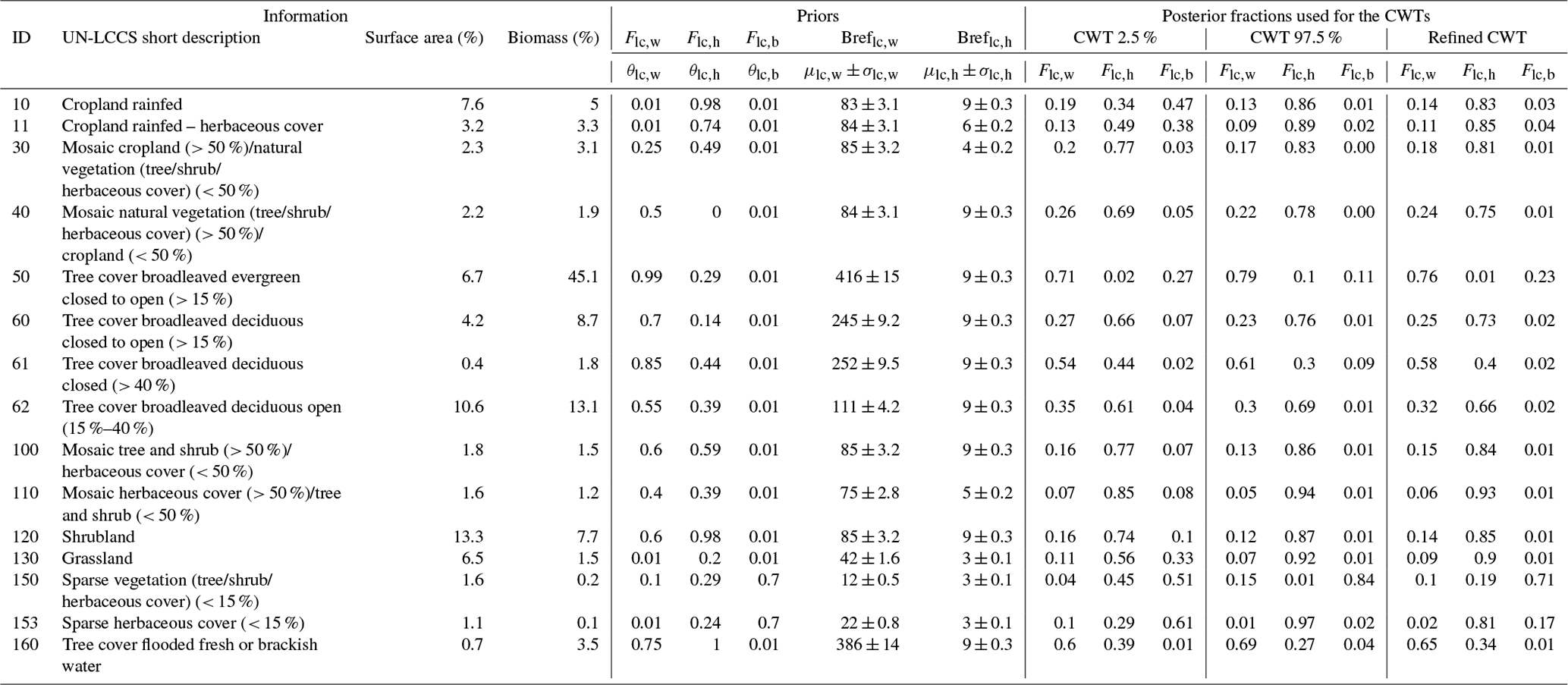
Given the spatial domain of this study, only the 31 land cover types defined on the ESA CCI-LC map and present in Africa were retained. The complexity of the study was further reduced by removing all land types that cover less than 1.0 % (304 158 km²) of the African surface or that contain less than 1 % (i.e., 1.1 Gt) of the total AGB of Africa. Filtering retrained 15 out of the 31 land cover types including bare land. These 15 land cover types (Table 1) represent 96 % of the surface of Africa and 98 % of its AGB.

Table 1 Description of the 15 PFTs used in ORCHIDEE to represent global vegetation.

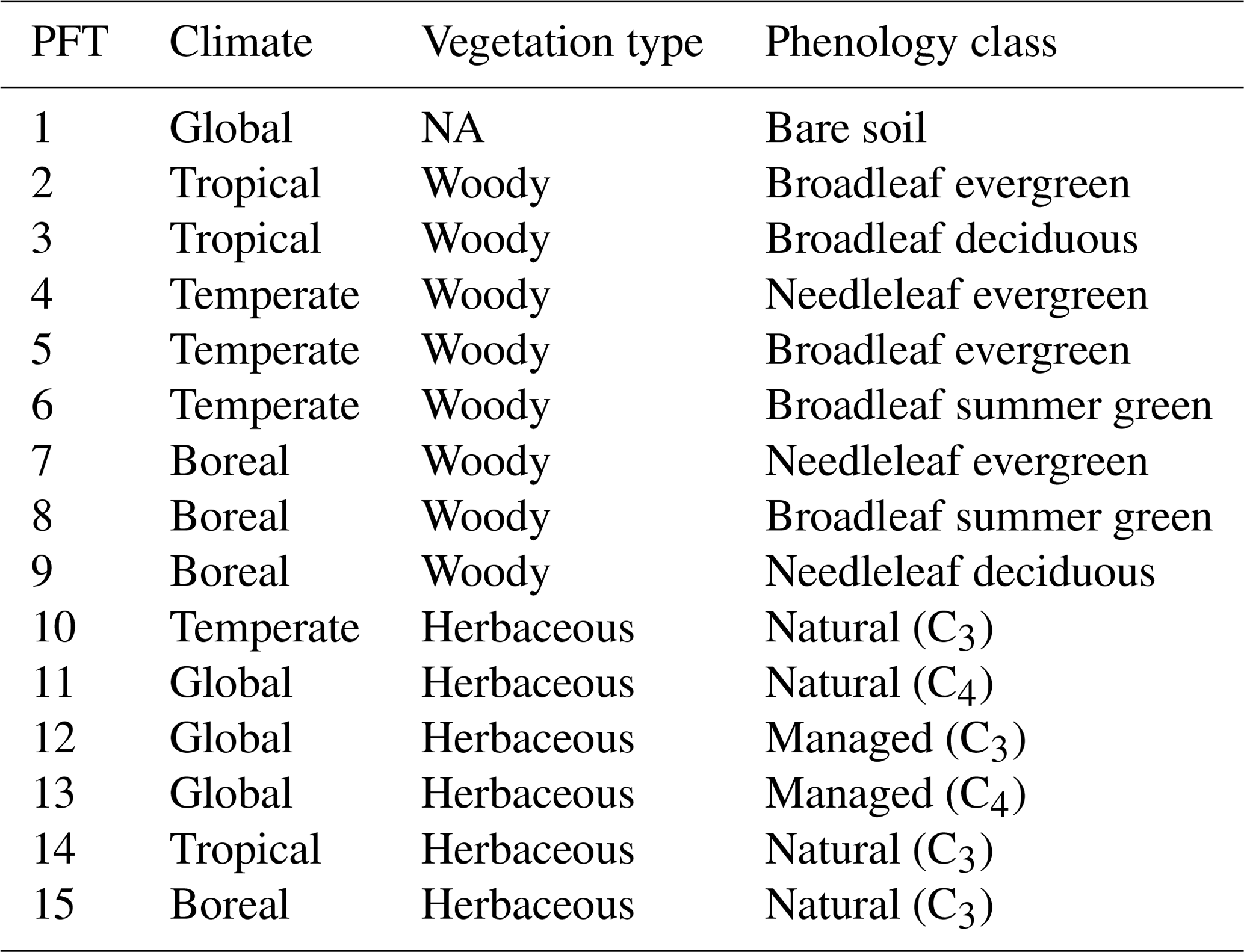
NA: not available.

One additional issue had to be dealt with the spatial resolution of the land cover map (9 ha) largely differed from the resolution of the AGB map (0.01^∘ × 0.01^∘, 100 ha). Therefore, each observational point on the AGB map is represented by 11 pixel × 11 pixel on the land cover map. To simplify the overall data assimilation methodology (see Sect. 3.2), we chose to use only AGB pixels (100 ha) which have a unique land cover type (i.e., pure pixels, in terms of land cover type). To this aim, the variety of land cover types across the 11 pixel × 11 pixel within each AGB pixel (i.e., the number of present LCT) was calculated, and only pixels where LCT=1 were retained. Although this criterion resulted in discarding 99 % of the pixels, each of the 15 land cover types considered could be represented by at least 2000 pixels. To remove outlier pixels, we choose to pick up the 2000 pixels strictly below the biomass value representing the 97.5th percentile of each land cover type (LCT) biomass distribution shown in Fig. 2.

Figure 2 Probability density distribution of the pure land cover pixel for biomass concentration Bp_p for 15 selected land cover types. The dashed line represents the 97.5th percentile used as the prior estimate for the reference biomass concentration for trees Bref_lc,w. The dashed line represents the 50th percentile also used as the prior estimate for the reference biomass for herbaceous cover.

2.3 Data assimilation

2.3.1 Linking land cover fractions and AGB

A linear model was used to relate the satellite-based AGB of a 100 ha pixel to the cover fraction of the satellite-based vegetation types present at the same location. This relationship can be written as

$$\begin{array}{}\text{(1)}& B_p={\sum }_{i=\mathrm{1}}^{n_{\mathrm{V}}}{F}_{p,i}\cdot {\text{Bref}}_i,\end{array}$$

where B_p is the AGB at a given pixel p, F_p,i is the cover fraction of the vegetation type i (i.e., the generic PFT used for land surface models; see Sect. 2.1 – overview), Bref_i is the reference AGB for the vegetation type i, and n_V is the number of vegetation types (i.e., number of PFTs) present in the pixel p. Given the number of unknowns (n_V being usually above 1), Eq. (1) has many solutions, many of which have no biological meaning. The equifinality of this model can be reduced by arguing that the large difference in biomass between woody, herbaceous and non-vegetated ecosystems combined by their respective cover fraction explains most of the biomass at pixel level. Following this assumption, Eq. (1) can be simplified as

$$\begin{array}{}\text{(2)}& B_p=F_{p,\mathrm{w}}\cdot {\mathrm{Bref}}_{\mathrm{w}}+F_{p,\mathrm{h}}\cdot {\mathrm{Bref}}_{\mathrm{h}}+F_{p,\mathrm{b}}\cdot {\mathrm{Bref}}_{\mathrm{b}},\end{array}$$

where F_p,w, F_p,h and F_p,b are the fractions cover for woody vegetation (i.e., woody PFTs), herbaceous vegetation (i.e., grassland and cropland) and non-vegetated areas, respectively. Bref_w and Bref_h are the reference AGB of woody and herbaceous vegetation, respectively, while Bref_b = 0. Hence, F_p,h in Eq. (2) can be substituted according to $F_{p,\mathrm{w}}+F_{p,\mathrm{h}}+F_{p,\mathrm{b}}=\mathrm{1}$ to obtain

$$\begin{array}{}\text{(3)}& B_p=F_{p,\mathrm{w}}\cdot {\mathrm{Bref}}_{\mathrm{w}}+\left(\mathrm{1}-F_{p,\mathrm{w}}-F_{p,\mathrm{b}}\right)\cdot {\mathrm{Bref}}_{\mathrm{h}}.\end{array}$$

Although Eq. (3) no longer details which vegetation types i (i.e., PFTs) are present on each pixel p, it still has four unknowns and therefore cannot be solved analytically. Nevertheless, a statistical solution is within reach if F_p,w, F_p,b, Bref_w and Bref_h are estimated from a population of AGB observations containing several independent repetitions that largely exceeds the number of unknowns. In this study, over 2000 repetitions were available for each of the 15 land cover types that were retained following filtering (Sect. 2.2.3). The statistical solution will thus consist of four mean parameter values (i.e., F_p,w, F_p,b, Bref_w and Bref_h) for each of these 15 land cover types.

As described in Sect. 2.2.3, the selection of homogeneous AGB pixels, i.e., those which have a unique land cover class across the 11.11 underlying land cover sub-pixels, allows us to rewrite Eq. (3) as follows:

$$\begin{array}{}\text{(4)}& \underset{\mathrm{¯}}{{\text{Bp}}_p}=F_{\text{lc},\mathrm{w}}\cdot {\mathrm{Bref}}_{\mathrm{lc},\mathrm{w}}+(\mathrm{1}-F_{\text{lc},\mathrm{w}}-F_{\text{lc},\mathrm{b}})\cdot {\mathrm{Bref}}_{\mathrm{lc},\mathrm{h}},\end{array}$$

where $\underset{\mathrm{¯}}{{\text{Bp}}_p}$ is the average AGB of a specific land cover type lc and F_lc,w, F_lc,b, Bref_lc,w and Bref_lc,h are the unknowns. The unknown parameters of the regression model (Eq. 4) were estimated by using a Bayesian inference method. This approach has been chosen because it helps to synthesize various sources of information as well as to propagate credible intervals in the result of our land surface model (Ellison, 2004). Bayesian inference requires, however, setting prior probability distributions for each of the unknowns, i.e., the biomasses and land cover fractions for each of the 16 land cover types. Given these prior probability distributions, Bayesian inference retrieves the posterior probability distribution for each of the unknown parameters.

2.3.2 Prior value distributions for Bref_lc,w, Bref_lc,h and Bp_p

The AGB pixels were stratified according to their land cover type and for each land cover type the information contained in the distribution of the satellite-based AGB served to estimate the mean and standard deviation of the prior values of Bref_lc,w. To avoid negative Bref values, we used a normal truncated distribution with $\mathrm{0}<a,b<+\mathrm{\infty }$, where (a,b) indicate the truncated range:

$$\begin{array}{}\text{(5)}& {\mathrm{Bref}}_{\mathrm{lc},\mathrm{w}}\sim N({\mathit{\mu }}_{\text{lc},\mathrm{w}},{\mathit{\sigma }}_{\text{lc},\mathrm{w}},a,b),\end{array}$$

where μ_lc,w is calculated as follows:

$$\begin{array}{}\text{(6)}& {\mathit{\mu }}_{\text{lc},\mathrm{w}}=X\text{th per }\left(\underset{\mathrm{¯}}{\mathit{B}{\mathit{p}}_{\text{lc}}}\right),\end{array}$$

where Bp_lc is a vector containing Bp_p values that belong to the land cover type lc, and Xth per denotes the 97.5th percentile for the woody cover types. This choice assumes that with the 97.5th percentile, we select the AGB value of a pixel covered only by woody vegetation (i.e., woody PFT) for the selected land cover type. In contrast to using a few in situ observations to define μ_lc,w, our approach offers the advantage to rely on a large ensemble of satellite-derived AGB observations and to be coherent with the following optimization.

Without any information about the variability of Bref_lc,w, we choose to represent σ_lc,w as

$$\begin{array}{}\text{(7)}& {\mathit{\sigma }}_{\text{lc},\mathrm{w}}={\mathit{\mu }}_{\text{lc},\mathrm{w}}\cdot \mathrm{0.0375},\end{array}$$

where 0.0375 accounts for a 30 % uncertainty encompassed between the interquartile range of the normally distributed Bref_lc,w. Compared to Bref_lc,w, Bref_lc,h is more difficult to assess from the satellite-derived data because it often shows bimodal distributions which may stem from biomass degradation or the presence of shrubs whose biomass better resembles that of a grassland than a woody ecosystem (Fig. 2). We found that while the 2.5th percentile is representing the lowest biomass for herbaceous ecosystem, the 50th percentile seems to better describe Bref_lc,h, following Eq. (6). Having no information about the variability of Bref_lc,h, σ_lc,w followed Eq. (7).

Finally, Bp_p, which was the 97.5th for woody cover types or the 50th percentile for herbaceous cover types, comes with a measurement uncertainty that was thought to follow a normal truncated distribution with $\mathrm{0}<a,b<{\mathrm{Bref}}_{\mathrm{lc},\mathrm{w}}$, where (a,b) indicate the truncated range. Given that this uncertainty is not known at the pixel level, an uninformative prior was set for the standard deviation σb_lc which can vary between 0 and 200 t ha⁻¹. We deliberately took a large uncertainty to cover the observation that considerable uncertainty remains in satellite-based biomass estimates (Bouvet et al., 2018):

$$\begin{array}{}\text{(8)}& \begin{array}{rl}{\text{Bp}}_p\sim N\left(\mathit{\mu },\mathit{\sigma }{b}_{\text{lc}}^{\mathrm{2}},a,b\right)& \text{ with }\mathit{\sigma }{b}_{\text{lc}}\sim U(\mathrm{0},\mathrm{200})\\ & \text{ and }\mathit{\mu }={\text{Bp}}_p.\end{array}\end{array}$$

2.3.3 Prior value distributions for F_lc,w, F_lc,b and F_lc,h

F_lc,w, F_lc,b and F_lc,h were defined as fractions of, respectively, woody vegetation, bare soil and herbaceous vegetation within a given land cover type; their values thus range between 0 and 1, and their sum is equal to 1. For this reason, a Dirichlet distribution was used to describe the probability distribution of the woody, bare soil and herbaceous cover fractions:

$$\begin{array}{}\text{(9)}& (F_{\text{lc},\mathrm{w}},F_{\text{lc},\mathrm{b}},F_{\text{lc},\mathrm{h}})\sim Di({\mathit{\theta }}_{lc,t},{\mathit{\theta }}_{\text{lc},\mathrm{b}},{\mathit{\theta }}_{\text{lc},\mathrm{h}}).\end{array}$$

OpenBUGS (Thomas, 2010), the software that was used in this study, cannot use a Dirichlet distribution as a stochastic node. This constraint can be overcome by making the cover fractions dependent on each other:

$$\begin{array}{}\text{(10)}& {\displaystyle }{F}_{\text{lc},\mathrm{w}}=q_{\text{lc},\mathrm{1}}\text{(11)}& {\displaystyle }{F}_{\text{lc},\mathrm{b}}=q_{\text{lc},\mathrm{2}}\cdot (\mathrm{1}-q_{\text{lc},\mathrm{1}})\text{(12)}& {\displaystyle }{F}_{\text{lc},\mathrm{h}}=(\mathrm{1}-q_{\text{lc},\mathrm{1}})\cdot (\mathrm{1}-q_{\text{lc},\mathrm{2}}).\end{array}$$

Let q_lc,i, with $i=\mathrm{1},\mathrm{\dots },K-\mathrm{1}$ and K the number of fractions, be a series of independent beta distributions, Be (α_i,β_i).

$$\begin{array}{}\text{(13)}& q_{\text{lc},i}\sim \text{Be}({\mathit{\alpha }}_{\text{lc},i},{\mathit{\beta }}_{\text{lc},i})\end{array}$$

The parameters of the beta distribution of the cover fraction of bare soil, woody vegetation and herbaceous vegetation (Eq. 9) can then be estimated as follows:

$$\begin{array}{}\text{(14)}& {\displaystyle }{\mathit{\alpha }}_{\text{lc},i}={\mathit{\theta }}_{\text{lc},i}\cdot ({\mathit{\omega }}_{\text{lc},i}-\mathrm{2})+\mathrm{1}\text{(15)}& {\displaystyle }{\mathit{\omega }}_{\text{lc},i}\sim U(\mathrm{0},\mathrm{1000}),\end{array}$$

where θ_lc,i which represents the fraction of each land cover type taken from expert knowledge used to define the so-called CWT and taken from a recent update of the CWT. ω_lc,i was described by an uninformative uniform distribution and thus reflects the relatively low trust we have in the current CWT. The dependencies between the beta distributions come from β_lc,i, which is estimated as

$$\begin{array}{}\text{(16)}& {\mathit{\beta }}_{\text{lc},i}={\sum }_{u=i+\mathrm{1}}^K{\mathit{\alpha }}_{\text{lc},u}.\end{array}$$

2.4 Credible interval propagation

2.4.1 Propagating the credible interval from the CWT into the PFT map

The posterior estimates of the cover fractions ($F_{\text{lc},\mathrm{w}},F_{\text{lc},\mathrm{b}},F_{\text{lc},\mathrm{h}}$) will be directly used to make up a new cross-walking table. The posterior estimates of the cover fractions values are then used to recalculate woody and herbaceous fraction of each generic PFT of the CWT. In other words, we keep the original split of the different woody PFT defined in the prior CWT and only rescale the total woody fraction to F_lc,w. Then we rescale the bare soil fraction based on F_lc,b to finally rescale short vegetation PFTs (grass and crop).

Given that these posterior estimates come with a probability distribution, a probability distribution of the CWT could be made. In this study, the 2.5th and 97.5th percentiles and the mode, i.e., the most common value, of the posterior estimates were used to create three cross-walking tables that were then applied on the ESA-CCI-LC product to create two PFT maps that represent the 95 % interval confidence of the ESA-CC-LC product and one PFT map which represents the one that is used in an ORCHIDEE simulation. The impact of the various PFT maps was quantified for simulated aboveground biomass and simulated surface albedo by running three simulations that only differed by the PFT map used to initialize the ORCHIDEE land surface model.

In the study, the uncertainty propagation index aimed to identify the ecoregions where the AGB and surface albedo estimates are most sensitive to uncertainties from the PFT map. This sensitivity was calculated as

$$\begin{array}{}\text{(17)}& S_{\text{eco},\mathrm{b}}={\displaystyle \frac{\text{ABS}(X^{\mathrm{97.5}}-X^{\mathrm{2.5}})}{\text{ABS}\left(F_{\text{eco},\mathrm{b}}^{\mathrm{97.5}}-F_{\text{eco},h}^{\mathrm{2.5}}\right)\cdot \mathrm{100}}},\end{array}$$

where X stands for AGB (t ha⁻¹) or surface albedo (unitless), and S_eco,b is expressed in the unit of X for a 1 % change in bare soil fraction.

2.4.2 Description of the ORCHIDEE land surface model

ORCHIDEE (Krinner et al., 2005; Boucher et al., 2020) is the land surface model of the IPSL (Institut Pierre Simon Laplace) Earth system model. Hence, by conception, it can be coupled to a global circulation model. In a coupled setup, the atmospheric conditions affect the land surface which, in turn, affects the atmospheric conditions. However, when a study focuses just on changes in the land surface ORCHIDEE rather than on the interaction with the atmosphere, it also can be run as a stand-alone land surface model. The stand-alone configuration receives atmospheric conditions such as temperature, humidity and wind, to mention a few, from the so-called meteorological forcing. The resolution of the meteorological forcing determines the spatial resolution and can cover any area ranging from a single grid point to the entire globe.

Although ORCHIDEE does not enforce a spatial or temporal resolution, the model does use a spatial grid and equidistant time steps. The spatial resolution is an implicit user setting that is determined by the resolution of the meteorological data. ORCHIDEE can run on any temporal resolution; however, this apparent flexibility is restricted as the processes are nested and formalized at given time steps: half-hourly (i.e., photosynthesis and energy budget), daily (i.e., net primary production) and annual (i.e., vegetation dynamics). Hence, meaningful simulations have a temporal resolution of 1 min to 1 h for the energy balance, water balance and photosynthesis calculations. In the land-only configuration used in this study, the default time step for these processes is 30 min.

When an application requires the land surface to be characterized by its actual vegetation, the vegetation will have to be prescribed by annual land cover maps. These maps must follow specific rules for the land surface models to be able to read them. In the case of ORCHIDEE, the share of each of the 15 possible plant functional types needs to range between 0 and 1 and be specified for each pixel. When satellite-based land cover maps are used as the basis for an ORCHIDEE-specific PFT map, the satellite-based land cover classification will need to be converted to match the ORCHIDEE specifications. As mentioned already above, this involves two steps: (i) the derivation of generic PFTs from the satellite land cover classes (in our case, the ESA-CCI-LC product) through the CWT discussed in this paper and (ii) the final mapping of the generic PFTs into the 15 ORCHIDEE-specific PFTs using additional information on the bioclimatic zones and the partition of grassland/crops into the C₃ versus C₄ photosynthetic pathway (Lurton et al., 2020).

In this study, AGB was defined as the sum of leaf biomass, fruit biomass, aboveground sapwood biomass and aboveground heartwood biomass, which are default output variables of ORCHIDEE. Surface albedo was defined as the albedo in the visible wavelengths and is a default output variable of ORCHIDEE.

2.4.3 Experimental setup

ORCHIDEE tag 2.0 (rev 6592) was used to run tree simulations that only differed by the PFT map used. Following a 340-year long spinup to initialize the carbon pools in the model, each simulation consisted of a 110-year long simulation between 1901 and 2010 with the Climate Research Unit – National Centers for Environmental Prediction (CRU-NCEP) v8 climate reconstruction (Viovy, 2017) that matched the simulation years. CO₂ concentration was fixed to 299.16 ppm and thus corresponds to the 2010 concentration.

2.4.4 Ecoregions

Results related to the land surface model simulation were presented by subdividing the African continent into ecologically homogeneous regions, so-called ecoregions, as defined by Olson et al., (2001).

Table 2 Surface area (%), share in the continental biomass (%), prior parameters and posterior median and credible interval values for each of the 15 land cover types considered in this study. The numbering, description and surface area of each land cover type are based on the ESA-CCI product (Defourny, 2019), where its share in the continental biomass is based on a compilation of Bouvet et al., 2018. θ_lc,μ_lc and σ_lc represent the parameters describing the prior distributions of F_lc and Bref_lc. Estimation of these parameters is detailed in Sect. 2.3. For each land cover type and each parameter, the 2.5th and the 97.5th percentiles are computed. We use the mode for the constrained CWT as an approximation of the posterior θ_lc,w, since the posterior distributions of F_lc,i may be asymmetric.

3 Results

3.1 Prior and posterior distributions estimates

3.1.1 Vegetation cover fraction: prior and reference biomass distributions

Prior distributions for the cover fractions and reference biomasses were determined for all 15 land cover classes separately; nevertheless, four broadly different groups could be distinguished: (1) the 97.5th percentile of biomass distribution for each land cover belonging in the first group was so high, i.e., from 245 to 416 t ha⁻¹, that the land cover types in this group must correspond to a substantial tree cover., i.e., a woody cover fraction from 0.58 to 0.75. Examples of this group are land cover types UN-LCCS 50, 61 and 160 (tree cover broadleaf types in Table 2). (2) Contrary to the first group, the 97.5th percentile of biomass distribution for each land cover type of the second group is so low, i.e., from < 12 to 42 t ha⁻¹, that these land cover types must be dominated by grasses or bare soil, i.e., a woody cover fraction of 0.1 or less and a substantial bare soil cover fraction up to 0.71. Examples of this group are UN-LCCS 130, 150 and 153 (grassland and sparse vegetation in Table 2). (3) The biomass of the third group falls in between these extremes representing mosaic land cover types like the UN-LCCS 10, 11, 30, 40, 100, 110 and 120 (mosaic landscape in Table 2). When taken over the African continent, the biomass distribution of these land cover types shows bimodal biomass distributions indicating considerable variability within these land cover types (Fig. 2). (4) The bimodal biomass distribution of the fourth group is backed by a rather high woody reference biomass associated with a low woody cover fraction which may represent an ecosystem highly disturbed by either silvicultural practice or a fire regime. UN-LCCS 60 and 62 fall into this group, which represents the woodland to dry savanna continuum.

3.1.2 Vegetation cover fraction: posterior distributions

Due to the Bayesian approach, the woody and herbaceous fraction within each land cover type is no longer deterministic (as was the case with the previous generation of cross-walking table such as in Poulter et al., 2015) but now comes with a distribution. This distribution is the outcome of propagating the credible interval on the retrieved parameters obtained from the Bayesian approach into the final product, i.e., the PFT cover fraction map. The 95 % credible interval was studied by comparing the 2.5th and 97.5th percentiles of the distribution of woody, herbaceous and bare soil fractions ($F_{\text{lc},\mathrm{w}},F_{\text{lc},\mathrm{h}},F_{\text{lc},\mathrm{b}}$).

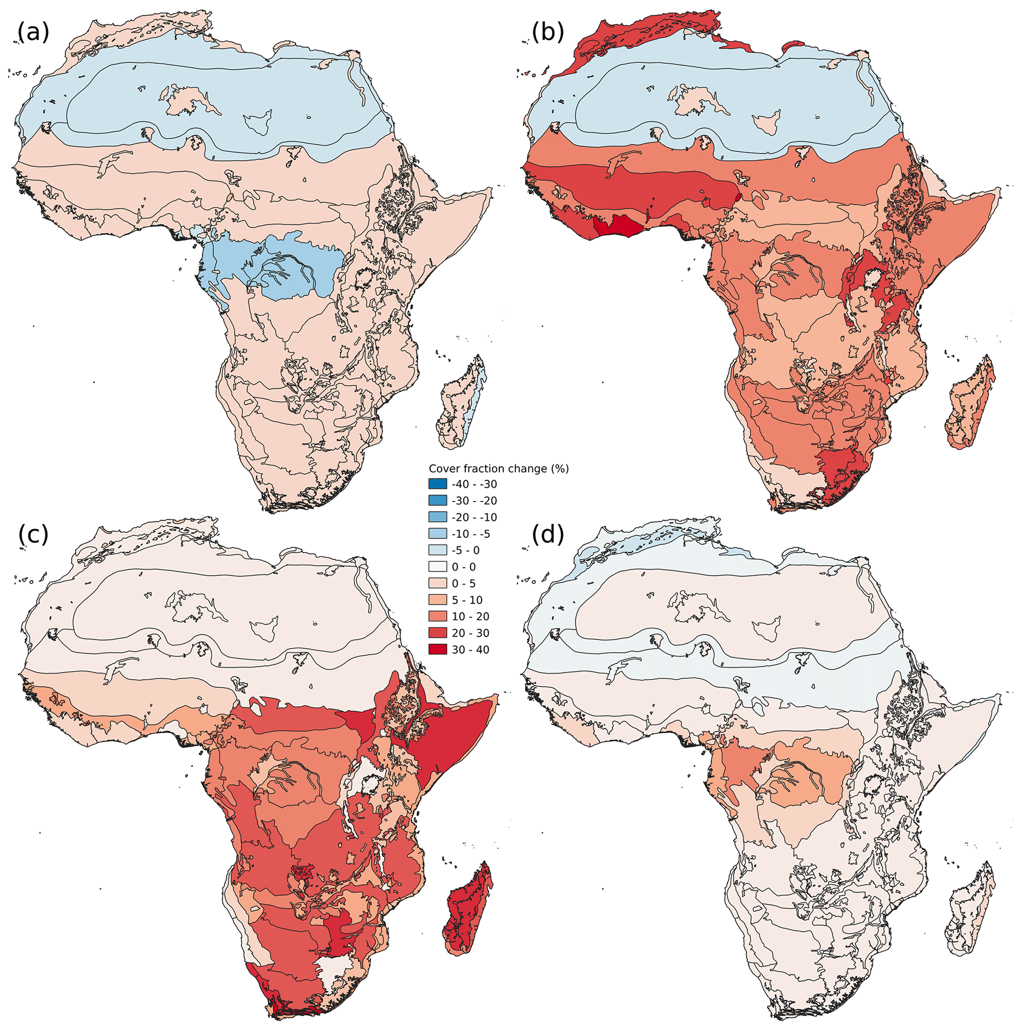
Figure 3 Uncertainty in CWT constrained by an AGB map. Absolute change in forest (a) and bare soil (b) cover fraction (%) between the 2.5th and 97.5th percentile PFT maps. High values represent a large uncertainty in the estimation of the true cover fraction. Panels (c) and (d) represent disagreement estimated as the difference between the CWT based on expert knowledge and the CWT constrained by an AGB map. Disagreement in forest (c) and bare soil (d) is expressed as absolute change (%). High values represent a strong disagreement between the two methods. Black lines delimit the different ecoregions according to Olson et al. (2001).

The mean change in forest cover fraction between the 2.5th and 97.5th percentiles of the distribution of constrained PFT maps over Africa was 1.6 ± 2.6 %. At the ecoregion scale (when averaging the cover fraction over the ecoregion), the largest uncertainty in forest cover fraction was found in the Congo Basin with an average of −6.3 ± 0.5 % for the six ecoregions where LCT 50 is dominant (Fig. 3a).

The 95 % uncertainty interval for bare soil cover fraction is 13 ± 8 % mainly due to the large uncertainty of the cropland and mosaic cropland (UN-LCCS 10, 11, 30, 40). In ecoregions where these LCTs are dominant, this credible interval increases to 24 ± 7 % (Fig. 3b). Moreover, dense forest land cover type, i.e., LCT 50 and 160 also come with 15 ± 4 % uncertainty in their bare soil fraction estimates (Fig. 3b).

Nonetheless, in a classic simulation experiment, the most common values of $F_{\text{lc},\mathrm{w}},F_{\text{lc},\mathrm{h}},F_{\text{lc},\mathrm{b}}$ will be used. The most common values of $F_{\text{lc},\mathrm{w}},F_{\text{lc},\mathrm{h}},F_{\text{lc},\mathrm{b}}$ are given by the mode of the posterior distribution (“constrained CWT” in Table 2). The mode was used to show the difference between the original and the constrained PFT maps (Fig. 3c and d). The mean difference in forest cover fraction between the prior (original) and the constrained PFT maps is −15 ± 12 % (Fig. 3c). Largest disagreement between was observed over the Somali acacia–Commiphora bushlands and thickets and the Kalahari xeric savanna where forest cover fraction was found to be on average 32 ± 1 % lower in the constrained PFT maps (Fig. 3c). The bare soil cover fraction changes on average by 3.1 ± 0.5 % (Fig. 3d). The constrained PFT map has on average 16 ± 4 % more bare soil cover fraction over the Congo Basin than the original map (Fig. 3c).

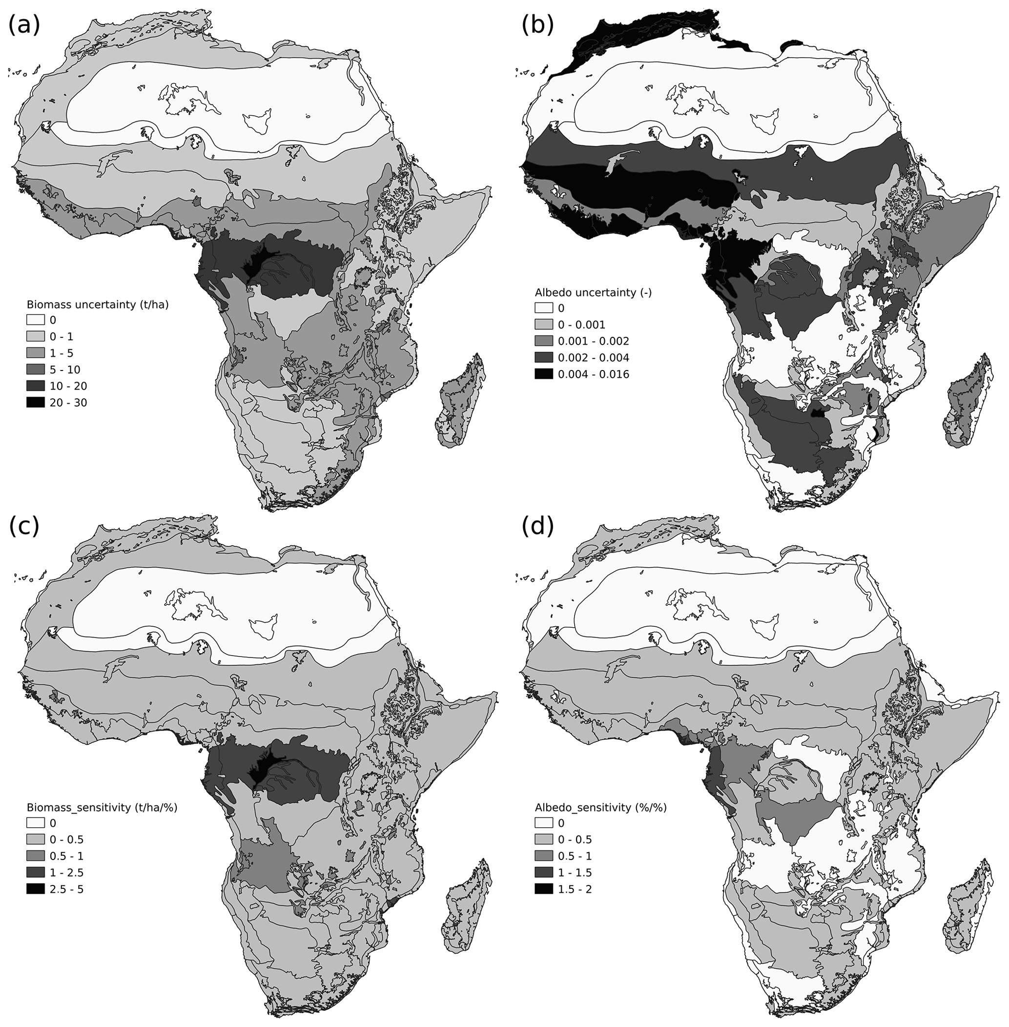
Figure 4 Confident interval propagation of the PFTs maps into AGB and visible albedo simulated by ORCHIDEE. (a) Uncertainty propagation into AGB and (b) uncertainty propagation into visible albedo from the difference between the 2.5 % and the 97.5 % PFT map defined by the optimization procedure. Uncertainty propagation index (Eq. 16) for AGB (c) and visible albedo (d).

3.2 Uncertainty propagation of the PFT maps on the aboveground biomass and visible albedo estimates from ORCHIDEE simulations

PFT maps are essential boundary conditions of land surface models because they condition the spatial distribution of various ecosystem state properties (i.e., carbon content, albedo, water–carbon–energy fluxes, etc.). When tested with ORCHIDEE tag 2.0 (rev 6592), the absolute difference in biomass stock between the 2.5th and 97.5th percentile maps was 0.5 ± 5.7 t ha⁻¹ (Fig. 4a) representing 0.2 $\mathrm{t}{\mathrm{ha}}^{-\mathrm{1}}{\mathrm{\%}}^{-\mathrm{1}}$ of cover faction (Fig. 4c). A notable exception is the Congo Basin where different PFT maps could result in AGB estimates that differ by 18 t ha⁻¹ (Fig. 4a) for a 6.5 % difference in the forest cover (Fig. 3a). Different PFT maps make the average visible albedo range from 0.081 ± 0.055 to 0.083 ± 0.055. The largest uncertainty for the visible albedo simulated with ORCHIDEE was found over the Nigerian lowland forest (0.158) and West Sudanian savanna (0.107) (Fig. 4b), which represent a 24 % to 11 % change in forest cover, respectively. The sensitivity is the highest in the western Congo Basin with 1.4  % of albedo %⁻¹ of cover faction. In contrast, the West Sudanian savanna possesses a low sensitivity with 0.5 %. To summarize, we found that a smaller forest to bare soil transition uncertainty can drastically change the albedo of an ecoregion than a larger uncertainty in the grassland/cropland to bare soil transition.

4 Discussion

4.1 Discretizing vegetation

Irrespective of the data products, the methods and the model used, discretizing vegetation comes with its own challenges. Discretizing transitions of ecosystems into land cover type classes (Sankaran et al., 2005), for example, can lead to systematic uncertainties since all pixels that belong to the same land cover class will get the same vegetation cover fractions in the cross-walking table (see Sect. 2.2.1). This approach articulates a key assumption underlying the PFT approach, i.e., that only one life form survives and thus dominates the vegetation due to competition for nutrients, light and water (Hutchinson, 1961). However, the savanna ecosystem, for example, is characterized by the coexistence of trees, shrubs and grasses which has been explained by interactions between vegetation, rainfall, fire and browsing regimes (Eigentler and Sherratt, 2020). This makes savannas one of the most difficult ecosystems to classify in a land cover type and subsequently convert it into a PFT map.

Over Africa, land cover classes such as shrubland (UN-LCCS 120) represent a wide range of ecosystems, from sparse xeric shrubland composed of small bushes, e.g., Penzia incana (Thunb.) Kuntze, grasses, e.g., Sip agrostis spp. such as found in the Karoo desert, to dense thicket composed by succulents, e.g., Portulacaria afra Jacq. and spinescent shrubs (∼ 3 m tall) (Mills, et al., 2005). Combining land cover types and biomass maps showed that the shrubland pixels in Africa more often resemble sparse xeric shrubland than dense thickets. Improving the ability to simulate land surface properties of shrublands in a changing world, especially in Africa where shrub encroachment is an important land cover dynamic (Wigley et al., 2009; Buitenwerf et al., 2012. O'Connor et al., 2014), is likely to benefit from a more detailed representation of shrublands in land surface models. A first step could be to represent shrubs as small trees, as was tested with the ORCHIDEE model for arctic ecosystems (Druel et al., 2017), but ultimately the control of precipitation on plant density (Rietkerk et al., 2002) should also be modeled.

Another major challenge with discretizing vegetation is how degraded ecosystems should be classified. From a modeling point of view, they should be classified as the land cover type that occurred prior to the degradation and the cause of the degradation, e.g., fire, grazing, erosion, should be explicitly accounted for in the land surface model. This ideal strongly differs from the current approach in which the degraded vegetation is classified as if it is in its natural state. Even when having the correct PFTs, the current approach would fail to simulate the observed biomass if degradation occurred. As an alternative, the PFT map could duplicate all PFTs to distinguish between a PFT in its natural state and in its degraded state. This approach in which degradation is accounted for in the PFT maps would, however, reduce degradation to a binary problem rather than addressing its continuous nature.

4.2 Knowledge gain from using the AGB map

In the absence of an AGB map, previous efforts to build cross-walking tables (Poulter et al., 2015) had to rely in part on expert knowledge. That generation of cross-walking tables can be considered as the best-available knowledge in the absence of AGB data or other information on the land surface cover. The method developed and demonstrated in this study mostly relies on data but comes with its own assumptions and statistical complexities. The key assumptions are that (1) previous cross-walking tables (Poulter et al., 2015) are a reliable source to set the prior distribution for PFT cover, (2) the biomass map (Bouvet et al., 2018) is a reliable source to set the prior distribution of the reference biomasses, and (3) the land cover classification contains homogeneous land cover types (Defourny et al., 2019). A key question is thus whether the added complexity justifies the knowledge gained by jointly assimilating a land cover and a biomass map when producing a CWT.

Ideally this question should be addressed by assessing the reduction of the credible interval associated to the posterior distribution of the PFT map when using the AGB map to constrain the CWT (in comparison to a prior when no AGB is used). However, the present generation of CWTs without AGB information does not come with a distribution (except the attempt in Hartley et al., 2017), calling for an alternative approach to assess the knowledge gain. Given that the prior distribution of the cover fraction was based on the previous CWT, the difference between the prior and the posterior distributions can be considered as the knowledge gained from using AGB information. Following this reason, we seek to answer the question of whether the cover fraction used by the original cross-walking table falls outside the 95 % credible interval of our posterior estimate.

If the answer is no, the biomass map is more likely in agreement with the previous effort to estimate the original cross-walking table. If the answer is yes, adding the information contained in the satellite-based biomass maps is most likely in strong disagreement with the previous effort to estimate the original cross-walking table. The original CWT has a global extent, and the constrained CWT is only valid for Africa. Therefore, knowledge gains should be carefully interpreted as they may reflect trade-offs that had to be made previously to construct a global rather than regional CWT. Knowledge gains were assessed for “croplands”, “dense evergreen forests”, “woodlands and savannas” and “xeric shrublands and grasslands” separately.

4.2.1 Croplands (UN-LCCS 10, 11, 30 and 40)

Despite the cover fraction of woody vegetation on croplands being close to none in the original CWT, this study found that the four land cover types associated with croplands (UN-LCCS 10, 11, 30 and 40) are in fact covered with 11 % to 24 % woody vegetation (Table 2). This large difference in the presence of woody vegetation on croplands is also reflected in the biomass data, which suggest that there are two distinct but co-existing agricultural systems in Africa, i.e., one system with a low biomass and one around with a higher biomass.

The agricultural system with the low biomasses likely represents annually replanted crops such as millet, sorghum, wheat, sweet potatoes or cassava (FAO), with a maximum reported biomass between 10 and 15 t ha⁻¹ for high-input cropping associated with commercial production of cassava and sweet potatoes. These values are in line with values estimated as reference biomass (see Table 2). Nonetheless, 97 % of total cropland area in Africa is rainfed (Calzadilla et al., 2009) and most of Africa's agricultural land is used for subsistence or small-scale farming associated with low-input cropping which explains why the actual average biomass estimate from the Centre d'Etudes Spatiales de la Biosphère (CESBIO) map for cropland is between 2.0 ± 0.7 t ha⁻¹ (Fig. 2) and thus considerably lower than the potential production.

The high-biomass agricultural system which is estimated at 83 ± 3 t ha⁻¹ in the CESBIO map (Fig. 2) likely includes plantations for coffee, rubber and fruits, as well as shelter trees and forest remnants (FAO). Permanent croplands do not have their own land cover type in the UN-LCCS or in ORCHIDEE. The mixture of bare soil, herbaceous vegetation and woody vegetation makes it challenging to discretize African croplands into the current PFTs (Table 1). Moreover, small changes in the woody reference biomass for high-biomass agricultural systems lead to large changes in cover fractions of herbaceous vegetation and bare soil ratio. Without constraint reference biomass estimates, total biomass alone does not sufficiently constrain the share of woody vegetation. For the time being, high-biomass agricultural systems could be with a woodland fraction ranging from 9.0 % to 26 % (Table 2). Although this could be an acceptable solution for biomass and albedo simulations, it will underestimate the agricultural production in the region.

4.2.2 Tropical rainforest (UN-LCCS 50 and 160)

The woody cover fraction of tropical rainforest in the original CWT is close to 90 % and falls outside the credible interval of the posterior estimates, i.e., 71 % to 79 %. The lower cover fraction from many pixels classified as tropical rainforest does not reach the reference biomass of 416 ± 16 t ha⁻¹ (Fig. 2). The reference derived from the biomass map matches the AGB observed at field plots of intact forests in the Congo Basin (Lewis et al., 2013) but the large value in bare soil cover fraction for these land cover types may thus reflect widespread degradation of the forests in the region (Tyukavina et al., 2018) or a too-high reference biomass (Kearsley et al., 2013).

4.2.3 Tropical deciduous forest, woodland and savanna (UN-LCCS 61, 60 and 62)

The woody cover fraction of the tropical deciduous forest ranged between 45 % and 75 % in the original CWT. Refining the CWT using AGB information shifts this range to between 27 % and 58 %. For savanna (UN-LCCS 62), the original cover fractions are within the constrained 95 % CI. For woody cover, the fraction of deciduous forest (UN-LCCS 61) decreased from 85 % to 58 %. We observe an overall decrease for the woody cover fraction since the reference biomass is much higher than the actual biomass of most of the pixels.

Although the reference biomasses used in this study are in line with previously reported values (Carreira et al., 2013), disagreement between the original and the constrained CWT is considerable. The original CWT starts from the view that all ecosystems (except croplands) are in their natural state. The AGB map, however, does not contain any evidence in support of this view but rather suggests that 50 % of the savanna (UN-LCCS 62) is 65 % below its reference biomass. Likewise, 50 % of dry woodland (UN-LCCS 60) is 71 % below its reference biomass (Fig. 2). The AGB map thus suggests widespread degradation of these ecosystems which are in a highly anthropized region (Mitchard et al., 2013). Uncertainty coming from the reference biomasses could be reduced by field observations at the ecoregion or finer spatial scales.

For deciduous forest, however, the difference in cover fraction of woody vegetation between the original CWT and the constrained CWT could also be explained by an inaccurate estimation of the reference biomass due to a too-coarse definition of the deciduous woody vegetation ranging from deciduous forest, over woodlands to savannas which are composed by different dominant tree species, with different biomasses (Sawadogo et al., 2010).

4.2.4 Xeric shrubland (UN-LCCS 100, 110 and 120)

The woody cover fraction of xeric shrublands and grasslands ranged between 40 % and 60 % in the original CWT. Accounting for the information contained in the AGB map, significantly decreased the woody cover fraction range toward 5.0 % and 16 %. Indeed, shrubs which represent a large part of the xeric shrublands were originally classified as woody vegetation for the ORCHIDEE model (i.e., when moving from the generic PFTs to the ORCHIDEE-specific PFTs; see Sect. 2). This assumption is true from an ecological point of view but in a simplified world like in land surface models, xeric shrubland has an aboveground biomass that resembles cropland and grassland (Fig. 2). By overlaying the land cover type and aboveground biomass maps, 37 % of the African shrublands were found to be degraded with a biomass of 2.7 ± 1.5 t ha⁻¹, 54 % were found to be intact with a biomass of 22 ± 19 t ha⁻¹ and 9 % of the shrublands are thickets with a biomass of 68 ± 11 t ha⁻¹. This is in line with other aboveground biomass estimates from remote sensing products (Saatchi et al., 2011; Mitchard et al., 2013; Avitabile et al., 2016) and in situ measurements where shrublands, degraded thicket and intact thicket in south Africa accumulated 3, 24 and 102 t ha⁻¹ of biomass, respectively (Mills, et al., 2005). These findings suggest that in the model world, xeric shrubland is best represented by a large fraction of herbaceous plant functional groups, when the overall objective is to model AGB.

4.2.5 Sparse vegetation (UN-LCCS 150 and 153)

The constrained cover fraction estimates are in line with the original CWT for UN-LCCS 150 which represent the most common class of sparse vegetation. The constrained cover fraction for UN-LCCS 153 has a larger herbaceous cover fraction, i.e., 29 % to 97 %, than the bare soil, i.e., 2.0 % to 61 % contrary to the original CWT. The herbaceous cover fraction could be overestimated if a too-low reference biomass was used. A reference biomass of 3.0 t ha⁻¹ was used and is acceptable compared to the reported biomass for the succulent and Nama Karoo biomes ranging from 0.5 to 7.6 t ha⁻¹ (Rutherford, 1978; Rutherford and Westfall, 1986). Given the current lack of reference biomass observations, disagreement between the original and constrained CWTs could be resolved by using an independent estimate of bare soil fraction.

4.3 Consequences for land surface modeling

4.3.1 Which land cover types affect the biomass estimate?

The large disagreement in cover fraction estimates (30 % to 40 %) resulted in small disagreement in biomass, i.e., < 1.0 t ha⁻¹ in regions with little precipitation like Somali acacia–Commiphora bushlands and thickets and the Kalahari xeric savanna. This counterintuitive result is explained by the growth processes simulated in ORCHIDEE. Under xeric climate conditions, ORCHIDEE simulates low tree biomasses (< 2.0 t ha⁻¹) because the low precipitation and subsequent plant water availability result in a continuous high tree mortality. Nonetheless, forest ecoregions like the eastern Guinean forests or in the Congo Basin, where the sensitivity to a change in the cover fractions ranged from 1.0 to 5.0 $\mathrm{t}{\mathrm{ha}}^{-\mathrm{1}}{\mathrm{\%}}^{-\mathrm{1}}$, had a considerable impact on the simulation since a 15 % uncertainty in the bare soil fraction may lead to a 75 t ha⁻¹ uncertainty of the biomass in the tropical forest of the Congo Basin. Underestimating the forest cover in humid ecoregions will have a much larger consequence on the simulated AGB than overestimating the forest cover in xeric ecoregions. The uncertainty surrounding the land cover fractions should thus be further reduced for the land cover types that already come with the lowest uncertainty, i.e., the forests.

4.3.2 Which land cover types affect the albedo estimate?

As for AGB, uncertainties in land cover fractions are only partly reflected in the uncertainties of the visible albedo. Dampening is caused by the fact that the reflectivities of grassland (0.06) and cropland (0.06) are close to the leaf reflectivity of a forest (0.03 to 0.04) compared to bare soils' reflectivity (0.1 to 0.25 depending on the color of the soil) in ORCHIDEE. By increasing the bare soil cover fraction, the albedo will increase accordingly but changing forest into grassland will not drastically change albedo. The most sensitive area is the western tropical forest in the Congo Basin for which a 15 % change in bare soil cover fraction may trigger a 15 % change in the visible albedo (Fig. 3c). Similar to that for AGB, the uncertainty surrounding the land cover fractions of the forested land cover types should be further reduced to reduce the uncertainty of the model simulations.

4.4 Outlook

In this study, a single biomass map was used as this enabled keeping the focus on the method itself. Nevertheless, other biomass products are available (Saatchi et al., 2011; Baccini et al., 2012; Avitabile et al., 2016; Santoro et al., 2021) and could have been used. Repeating this study for each of these biomass products would add another source of uncertainty to the cross-walking table. Due to the method presented in this study, this uncertainty could then be propagated into the PFT map and all the way up to the simulated biomass albedo as done in this study for one biomass product and other land surface properties. Considering different biomass products would give an insight of the impact of satellite-based biomass estimates on the discretization of the vegetation and by extension surface properties as estimated by land surface models. Likewise, a single land cover map has been used in our analysis, but other products are available as well (Copernicus, Xu et al., 2019; Li et al., 2020). By using different land cover maps, one could quantify the uncertainty in the land cover classification and propagate it to evaluate its impact on the simulated land surface properties.

Compared to that in other continents, the African vegetation has been documented by relatively few quantitative observations (Mills, et al., 2005; Saatchi et al., 2011; Asner et al., 2012; Réjou-Méchain et al., 2015). Hence, it is the continent where remote sensing data could largely enhance our knowledge on the issue. Recent high-resolution satellite observations bear the promise to significantly reduce the credible interval around the aboveground carbon stock to estimate the CO₂ emissions from tropical forests (Hansen et al., 2013; Bouvet et al., 2018; Defourny et al., 2019; Buchhorn et al., 2020) but land surface models will need to be ready to routinely assimilate these data to fully benefit from the information contained in biomass maps. This study demonstrated one way in which satellite-based biomass data can help modelers to constrain the initialization process by means of refining the cross-walking tables that are used to map land cover classes derived from satellite observations into PFT maps. Nevertheless, biomass maps could be used for applications other than model initialization (this study), including model parameterization and model evaluation.

The biomass map could be used to optimize model parameters related to growth, turnover and mortality to better simulate the vegetation biomass for the different PFTs. The evaluation stage could benefit from the biomass maps by benchmarking the model results against observed relationships between biomass–climate and biomass–land use to better distinguish and simulate the difference between actual and potential biomass (Sankaran et al., 2005). Although the availability of several biomass products makes it possible to use one product to inform the cross-walking tables and another product to evaluate the simulated surface properties, the magnitude of present-day differences between biomass products (Mitchard et al., 2013) is expected to result in major inconsistencies when different biomass products are used for different purposes (e.g., assimilation, parameterization, evaluation) into a single analysis. In this study, less than 0.01 % (see Sect. 2.3.1) of the information contained in the biomass map was used to constrain the cross-walking table and none was used to optimize model parameters. The simulated biomass remains, therefore, largely independent from the biomass map which implies that a single biomass map can be used for land cover optimization (as in this study) and in a second step for parameter optimization or model evaluation.

With an increase in resolution of the land cover map comes a decrease in the reliance on the cross-walking tables. Cross-walking tables will no longer be required once the resolution will be high enough (around 10 m × 10 m) such that each pixel contains a single vegetation type equivalent to a single PFT classification used by land surface models (Li et al., 2020). No longer having to rely on cross-walking tables would likely reduce the width of the credible intervals of the PFT map. As there would no longer be a need to estimate woody and herbaceous fractions, there would no longer be a need for the information contained in the biomass map. It will then be feasible to solely use biomass maps to better parameterize the processes that contribute to simulating the reference biomass. It should be noted, however, that higher resolutions will not solve the basic challenge of discretizing vegetation. High-resolution land cover maps would split structurally complex ecosystems, for example, savannas, into a pure forest fraction and a pure grassland fraction. This would overlook the interactions between the grasses and the trees which are among the defining ecological characteristics of a savanna.

Finally, we should note that other satellite-derived products than the AGB could be used to constrain the mapping of the land cover classes into model PFTs (i.e., CWT). For instance, the global tree cover fraction map, at 30 m resolution, from Hansen et al., (2013) could also be used to constrain the fraction of bare soil within each land cover class like what was done in this study with the AGB map.

5 Conclusion

This study demonstrates how an aboveground biomass map could be used to constrain a cross-walking table that enables remapping land cover types derived from satellite observations into plant functional types used as a boundary condition in land surface models. Given that previous cross-walking tables did not report uncertainties as they were mostly based on expert knowledge, it remains unclear how much the use of an additional constraint really improved the cross-walking tables. Nevertheless, the considerable uncertainties remaining in the cross-walking table that made use of the aboveground biomass map suggest that total biomass map should be complemented with a bare soil map to better constrain the cross-walking table. Likewise, the reference biomass for both herbaceous and woody vegetation needs to be constrained to at least the ecoregion scale to avoid underestimating or overestimating bare soil fractions. The method developed in this study helped to estimate the uncertainty of cross-walking tables which can now be used to benchmark further methodological developments. Moreover, the method identified bare soil cover fraction would be required to reduce the uncertainty of future cross-walking tables and the plant functional type maps they generate.