the Creative Commons Attribution 4.0 License.
the Creative Commons Attribution 4.0 License.
 | 25 Mar 2022
A global, spherical finite-element model for post-seismic deformation using Abaqus
Grace A. Nield
Matt A. King
Rebekka Steffen
Bas Blank
We present a finite-element model of post-seismic solid Earth deformation built in the software package Abaqus (version 2018). The model is global and spherical, includes self-gravitation and is built for the purpose of calculating post-seismic deformation in the far field ( km) of major earthquakes. An earthquake is simulated by prescribing slip on a fault plane in the mesh and the model relaxes under the resulting change in stress. Both linear Maxwell and biviscous (Burgers) rheological models have been implemented and the model can be easily adapted to include different rheological models and lateral variations in Earth structure, a particular advantage over existing models. We benchmark the model against an analytical coseismic solution and an existing open-source post-seismic model code, demonstrating good agreement for all fault geometries tested. Due to the inclusion of self-gravity, the model has the potential for predicting deformation in response to multiple sources of stress change, for example, changing ice thickness in tectonically active regions.
- Article
(4397 KB) - Full-text XML
- BibTeX
- EndNote


Earthquakes cause deformation at the Earth's surface from the immediate coseismic fault slip and, thereafter, from several processes. Afterslip on the fault on or near the rupture zone (e.g. Huang et al., 2014) and poroelastic relaxation due to changes in fluid pressure (e.g. Masterlark and Wang, 2002) result in deformation of near-field locations (typically <300 km from the fault). As the Earth responds to stress changes associated with the earthquake, the lower crust and upper mantle undergo prolonged post-seismic viscoelastic deformation. This is the dominant mode of displacement in the far field and, for very large earthquakes (> magnitude 9), this can be observed geodetically over 1000 km from the earthquake source (Shao et al., 2016) and be sustained over decades. For example, deformation from the 1960 magnitude 9.5 Chile earthquake was still being observed ∼40 years after the event (Khazaradze and Klotz, 2003). Post-seismic deformation can be observed by increasingly dense networks of geodetic measurements such as Global Positioning System (GPS) (e.g. Freed et al., 2012) and Interferometric Synthetic Aperture Radar (InSAR) (e.g. Wang and Fialko, 2018) motivating the development of models to help interpret geodetically observed deformation. The study of post-seismic deformation can provide useful information about the Earth and can be used to place constraints on the inferred Earth structure (Pollitz, 2005) or rheology (Freed et al., 2012). It is important to be able to accurately quantify post-seismic deformation in regions where deformation occurs as a result of multiple sources, for example, in Alaska where the Earth is also deforming in response to a changing ice load (Suito and Freymueller, 2009).
Post-seismic deformation has been studied using a variety of modelling techniques, from simple layered half-space (also known as “flat-Earth”) models to models that consider Earth's sphericity and three-dimensional material properties. For studying the far-field effects of earthquakes consideration of sphericity is required (Pollitz, 1992). Pollitz (1997) developed a software (VISCO1D, freely available from the USGS at https://www.usgs.gov/node/279413 (last access: March 2002), which contains a link to download the software) to calculate post-seismic deformation on a spherical layered Earth incorporating an Earth model that varies in the radial direction only. It uses viscoelastic normal mode theory and calculates deformation from spherical harmonic expansion of global modes of relaxation. Deformation can be calculated both with and without the effect of gravity, that is, the restoring forces within the Earth allowing it to regain gravitational equilibrium. The effect of including gravity is that deformation ceases once the Earth has adjusted to the change in stress, whereas without gravity, deformation continues. This model has been employed for a wide range of earthquake studies, such as constraining Earth properties and rheological behaviour in response to the magnitude 7.9 2002 Denali earthquake in Alaska (Pollitz, 2005), computing post-seismic gravity change following the magnitude 9.1 2011 Tōhoku earthquake gravity change (Han et al., 2014) and modelling post-seismic deformation of Antarctica (King and Santamaría-Gómez, 2016). Furthermore, VISCO1D has been used to benchmark other codes of post-seismic deformation calculation (Wang et al., 2006). Whilst VISCO1D is a powerful tool, it is limited to a one-dimensional Earth model which may not be appropriate for some studies where lateral variations in Earth structure may be required to fully explain geodetic observations (King and Santamaría-Gómez, 2016).
Several finite-element models of post-seismic deformation have also been developed (Freed et al., 2006; Masterlark et al., 2001; Takeuchi and Fialko, 2013), although the majority have been restricted to a half-space geometry. Hu and Wang (2012) updated their finite-element model (Hu et al., 2004) to include spherical geometry and used it to study the 2004 magnitude 9.2 Sumatra earthquake, where a spherical geometry allowed for more realistic slab and fault geometry to be included; however, they limited the spatial extent of the model to the case study region. Agata et al. (2019) modelled post-seismic deformation following the 2011 magnitude 9.0 Tōhoku earthquake with a finite-element model incorporating spherical (but not global) geometry, restricting the model domain to 2500 km by 2500 km to allow for a high-resolution mesh. Whilst limiting the spatial extent is computationally efficient and does not cause a problem for the estimation of post-seismic deformation, to compute a fully self-gravitational solution using spherical harmonics a full global model is required. Self-gravitation takes account of the change in gravity field caused by deformation and the redistribution of mass within the Earth. The effect of self-gravitation due to earthquake-related deformation is likely to be small for the majority of earthquakes, and not on the same scale as that caused by glacial isostatic adjustment since the magnitude of deformation is much smaller, but including it allows consistent modelling of deformation due to multiple sources (e.g. glacial cycles). Furthermore, for large earthquakes, the change in gravity field resulting from deformation and redistribution of mass within the Earth could be significant, and, if the earthquake occurs under the ocean, redistribution of water also contributes to the change in gravity and hence affects sea levels (Broerse et al., 2011).
The purpose of the model presented in this paper is to estimate far-field post-seismic deformation primarily from large earthquakes. The model is a global, spherical finite-element model constructed with the commercial software Abaqus (https://www.3ds.com/products-services/simulia/products/abaqus/ (last access: February 2019); Hibbitt et al., 2016). It is an improvement on existing models since it includes both global spherical geometry and the capability to use 3-D variations in Earth properties which can significantly affect viscoelastic deformation (e.g. Latychev et al., 2005; Zhong et al., 2003; Wu et al., 2013). Furthermore, the model has the potential to simultaneously include different sources of Earth deformation, for example, post-seismic deformation in a region undergoing, or which has previously undergone, surface-mass change (e.g. ice-mass change). This is needed, for instance, to separate present-day surface deformation signals observed by GPS.
This paper describes the model setup and the methods implemented to estimate coseismic and post-seismic deformation (Sects. 2 and 3). Since afterslip and poroelastic relaxation are considered only to affect deformation in the near field of the fault for all but the largest earthquakes (Peña et al., 2019), they are not included in our model. We benchmark model results for several simple scenarios against existing codes (Sect. 4) and discuss the advantages and limitations of the model (Sect. 5). The input files are available to allow other users to replicate results and use the methods to set up their own post-seismic deformation models.
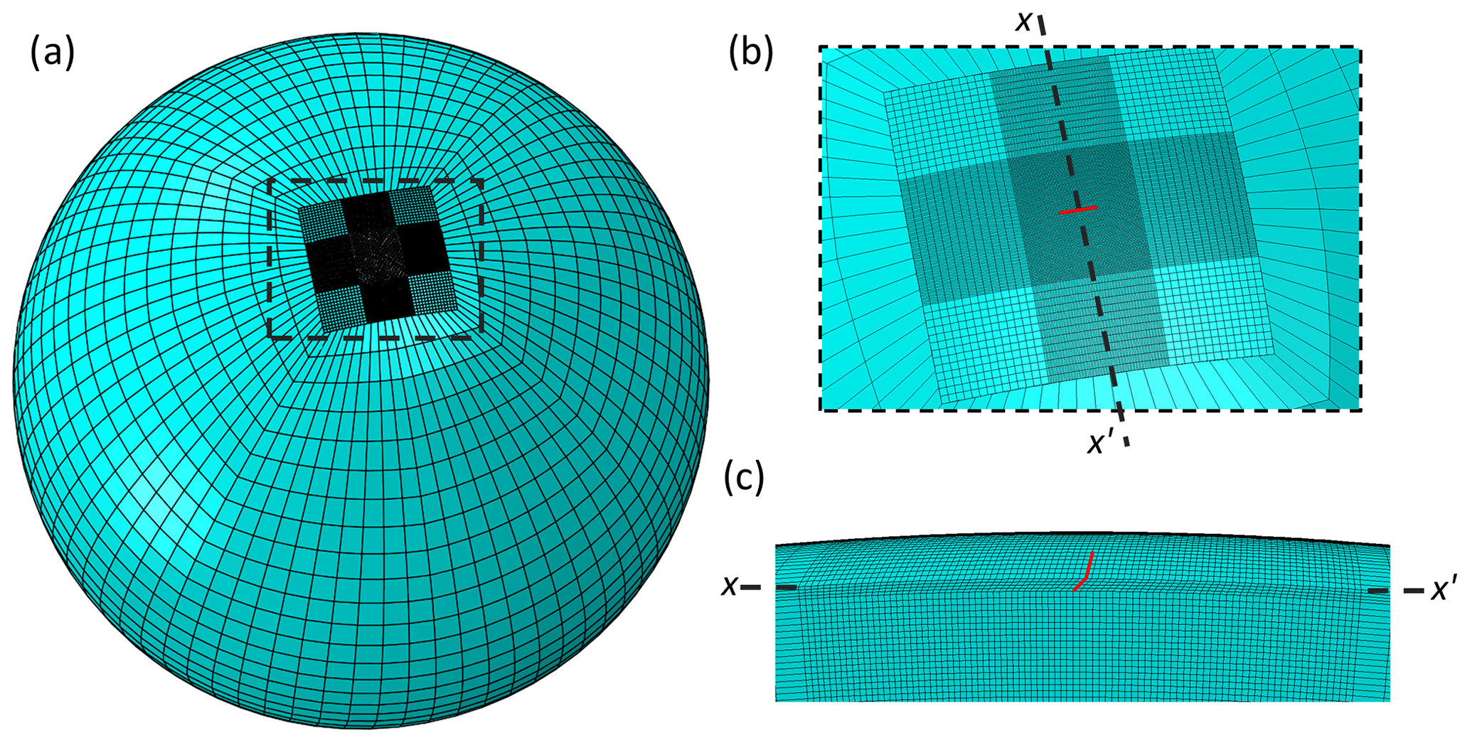
Figure 1Abaqus mesh; (a) full global mesh with high-resolution fault region surrounded by lower-resolution elements; (b) close-up plan view of the fault region with fault marked in red and cross section x–x′ shown in panel (c); (c) cross section x–x′ (as marked in panel b) through the fault region for 45∘ dipping fault with the fault marked in red.
2.1 Model geometry and mesh
The model is a global, spherical representation of the Earth, developed in Abaqus version 2018 but is also compatible with older versions of the software as well. It is based on the finite-element model for computing glacial isostatic adjustment following the methods described by Wu (2004), whereby we use the same setup of a viscoelastic Earth relaxing in response to a stress change, but instead of applying a changing ice-surface load we implement a fault and associated slip. We model a spherical Earth rather than taking a layered half-space approach so a more realistic geometry can be included and gravity perturbations due to deformation can be accounted for by means of a spherical harmonic expansion. The model has layers from the surface to the core–mantle boundary with computational feasibility being the only limit on the number of layers. Each layer is assigned material properties according to user requirements and would typically consist of an elastic outer layer representing the uppermost lithosphere, with viscoelastic lower lithosphere and mantle layers below.
An earthquake is simulated in the model by movement on a fault plane within the mesh (see Sect. 3 for details) and in order to compute deformation to a sufficient accuracy a high-resolution mesh is required in the vicinity of the fault. To balance the need for a high-resolution mesh against a model with a computationally feasible number of elements, we take the approach of constructing two separate parts (Abaqus keyword *PART): one for the high-resolution fault region and one for the lower resolution surrounding Earth (Fig. 1). The two parts are then tied together (Abaqus keyword *Tie) using surface-to-surface tie constraints. This means that although the two separate meshes have non-conforming elements relative to each other, the tie constraints ensure there is no relative movement between the surfaces and that displacement and stress are continuous through the boundaries. Tie coefficients are generated and used to interpolate quantities from nodes on one side of the mesh to nodes on the other side of the mesh. The size of the part containing the fault and high resolution mesh can be changed according to the requirements of the individual case study, and in the simulations presented in this study, is large enough to contain the far-field area of interest. The high-resolution mesh block extends to 670 km depth (i.e. the base of the upper mantle), so that any deformation that may be caused by the fault movement is within the block, and hence there is minimal stress to transfer across the tied surfaces. The element type used is an eight-node linear brick element (C3D8 in Abaqus).
2.2 Rheology and Earth parameters
All layers within the model are assigned a density (ρ), Poisson's ratio (ν) and Young's modulus (E) (Abaqus key words *Density *Elastic). For viscoelastic layers below the purely elastic outer shell, a relaxation time is specified which is based on a Prony time series (Abaqus key words *Viscoelastic). In this study, we limit our benchmarking examples to a 1-D linear viscoelastic rheology with one (Maxwell) or two (Burgers) relaxation times and include one example implementing the elastic properties of the widely used Preliminary Reference Earth Model (PREM, Dziewonski and Anderson, 1981). However, Abaqus has the capability to implement a variety of rheological models, including user-specified constitutive equations. For example, Freed et al. (2012) combined power-law rheology with a transient phase to model post-seismic deformation following the 1999 magnitude 7.1 Hector Mine earthquake, and van der Wal et al. (2010) used a composite rheology based on laboratory-derived flow laws for diffusion and dislocation creep (Hirth and Kohlstedt, 2003; Karato and Wu, 1993) to model global glacial isostatic adjustment. Furthermore, variations of our model could be constructed using a 3-D Earth structure (e.g. van der Wal et al., 2015) (more information on how this can be done is included in the the supporting material; Nield, 2022).
2.3 Boundary conditions
We follow the approach described in Sect. 4.1 of Wu (2004) and apply elastic foundations (Abaqus keyword *Foundation) to each layer boundary with a material density contrast occurring across it (including the surface and core–mantle boundary). This means that advection of pre-stress is included and takes care of the restoring forces of buoyancy neglected in a conventional finite-element model (Wu, 2004, Eq. 3). The elastic foundations have a stiffness equal to the difference in density multiplied by gravitational acceleration (see Wu, 2004, Eq. 12a–c). Schmidt et al. (2012) show that the use of foundations at surfaces not perpendicular to the direction of gravity produces errors in results, but we ensure that density contrasts occur only at spherical layer boundaries in our model which satisfies this requirement. The foundations could be also replaced by spring elements when an inclined density contrast is used (Schmidt et al., 2012).
2.4 Time steps
Once the model has been set up with the geometry, rheology, Earth parameters, boundary conditions and fault slip (see Sect. 3); time steps are created to run the model. The first step of the run is a static step to allow the fault to slip. In this step, all material properties are treated as elastic and the fault displaces immediately; hence, no actual time needs to be assigned. All subsequent steps are for the simulation of post-seismic relaxation and consequently must have a time assigned to them. One full run of all the time steps is one iteration.
2.5 Self-gravitation
Movement of mass due to deformation of the Earth perturbs the gravity field which in turn affects the Earth's deformation. The effect of changes in the gravity field needs to be taken into account to make the model self-gravitating. This is done iteratively as described in Sect. 4.3 of Wu (2004), first using a non-self-gravitating model and computing the resulting gravitational potential from the radial displacement using the equations presented in Sect. 4 of Wu (2004). Applying this as a new load at the interfaces of the model where a density contrast occurs across them, the displacement is recalculated (i.e. another iteration is run). Wu (2004, Sect. 4.3) suggests running the model for four to five iterations to achieve convergence of the solution.
2.6 Outputs
Abaqus can compute many different output variables depending on the model setup. For our model, the main output of interest is a global grid of deformation in the east, north and radial directions. It is also possible to output stress, strain and perturbation to the geoid which could be used to correct satellite gravimetry data for the gravity change associated with very large earthquakes (e.g. Han et al., 2014).
3.1 Fault geometry and slip
In our model, an earthquake is simulated by prescribing slip on a fault plane. In order to implement this in a finite-element mesh, we require two separate surfaces that can move relative to each other. We take the approach of Steffen et al. (2014), whose model simulates fault slip due to changes in stress during glacial cycles, whereby the fault plane geometry is created prior to meshing and then, once generated, the mesh is subsequently altered to produce two surfaces. This is accomplished by duplicating the nodes that lie on the fault surface and then reassigning the duplicated nodes to the elements on one side of the fault plane, thereby creating a “cut” in the mesh. Although the elements on each side of the fault are defined by different nodes, the node pairs initially have the same coordinates (Fig. 2).
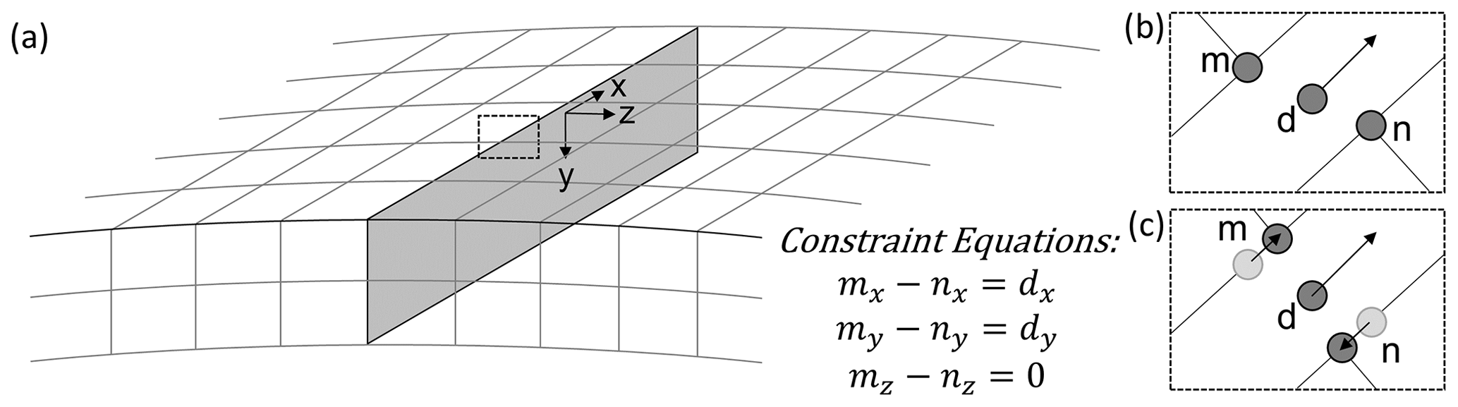
Figure 2(a) Diagram of the fault plane (shaded grey) in the Abaqus mesh with co-located node pairs and local coordinate system aligned with the fault plane; (b) close-up of a node pair (m, n) and dummy node (d) with displacement boundary condition applied in the x direction of the local coordinate system (for illustrative purposes only, the fault is not allowed to open in the z direction); (c) constraint equations applied to the node pair results in displacement of nodes m and n in the x direction.
The model of Steffen et al. (2014) incorporates a complex stress history comprising tectonic stresses and stresses relating to glacial cycles allowing faults to slip in response to the changing conditions. Our model differs from this approach because the amount of slip that occurs on the fault plane is prescribed. This negates the need to specify any fault surface parameters such as coefficient of friction or cohesion but does require detailed knowledge of the earthquake event. Prescribing an amount of slip on the fault plane is a reasonable approach as fault properties, such as length, width, strike, dip, rake and slip are often solved through independent means such as fault inversion studies (Hayes, 2017) and detailed fault slip information is not required when studying far-field deformation. Furthermore, we do not include any pre-stress in the model; that is, there is no tectonic or background stress applied before the fault slips. This has no effect for models that use Maxwell or Burgers rheology as they are independent of stress.
3.2 Coseismic slip
Once the finite-element mesh has been adjusted to accommodate the fault plane, coseismic displacement is prescribed following the approach of Masterlark (2003). For every node pair on the fault plane (i.e. nodes on either side of the fault that have the same coordinates), a third “dummy” node is created at the same location but not connected to any element in the mesh (Fig. 2). Dummy nodes are assigned a displacement boundary condition (Abaqus keyword *Boundary) in the x and y directions of a local coordinate system aligned with the fault plane (see Fig. 2) with the amount of displacement in each direction depending on the slip and rake. For example, using basic trigonometry, a slip of 5 m at a rake of −60∘ would equate to slip of 2.5 m in the x direction and 4.3 m in the y direction. Kinematic constraint equations (Abaqus keyword *Equation) are then constructed for each node pair and its corresponding dummy node which specifies the relative displacement between the node pair in the x and y direction. There is no relative displacement in the z direction of the local coordinate system (i.e. normal to the fault plane), as the fault is not allowed to open. Because the constraint equations are specified separately for each node, the fault plane can accommodate a spatially variable slip distribution. The first step of the model run is a static step (Abaqus keyword *Static) in which the nodes (and hence the fault plane) displace according to the kinematic constraint equations. During the static step, all materials are treated as elastic.
Table 1Fault geometry used in the three benchmarking exercises. Note that test case 3 is run with three Earth models; see Table 2.
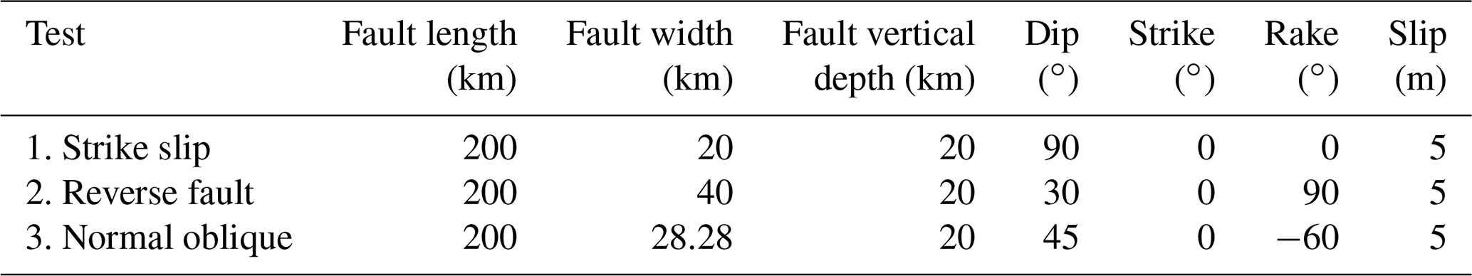
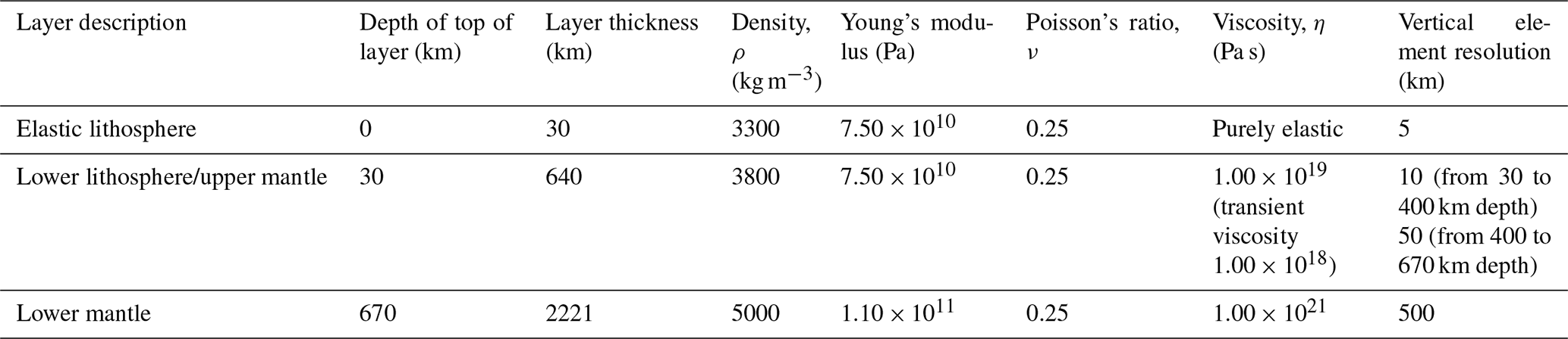
Table 2Earth model used in the Abaqus model for the benchmarking exercises with a Maxwell rheology and a Burgers rheology (transient viscosity given in brackets). The Maxwell viscosity profile is also used in conjunction with the PREM elastic structure for test case 3.
3.3 Post-seismic deformation
Following the first step of the model run (i.e. the earthquake), the subsequent time steps simulate post-seismic deformation (Abaqus keyword *Visco) by allowing the mesh to deform under the stresses caused by the displacement on the fault plane. The kinematic constraint equations remain in place throughout the model run which means that there is no further relative displacement between the node pairs.
In order to verify the model, we benchmark the results against those produced with the Okada analytical solution for coseismic displacement (Okada, 1985) and the VISCO1D code (version 3) for gravitational post-seismic relaxation (Pollitz, 1997).
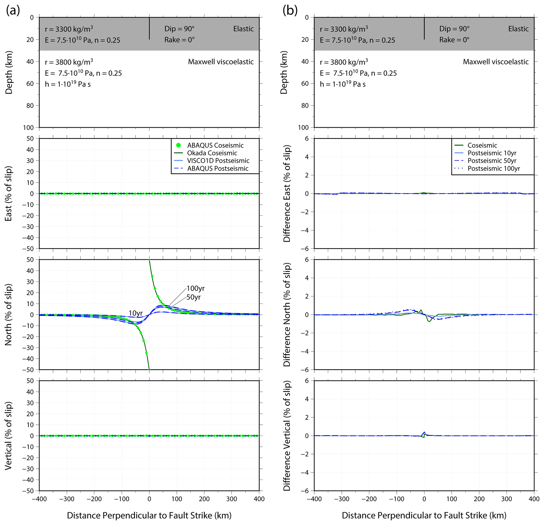
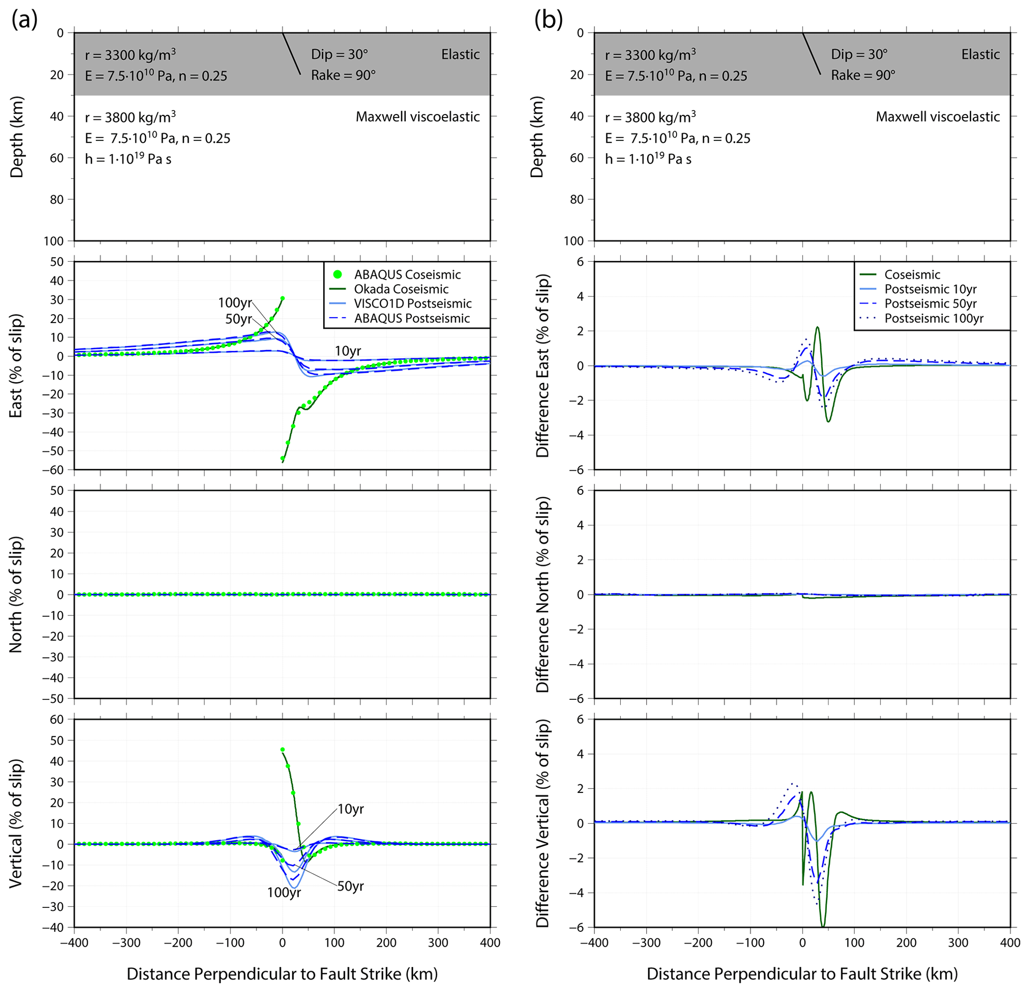
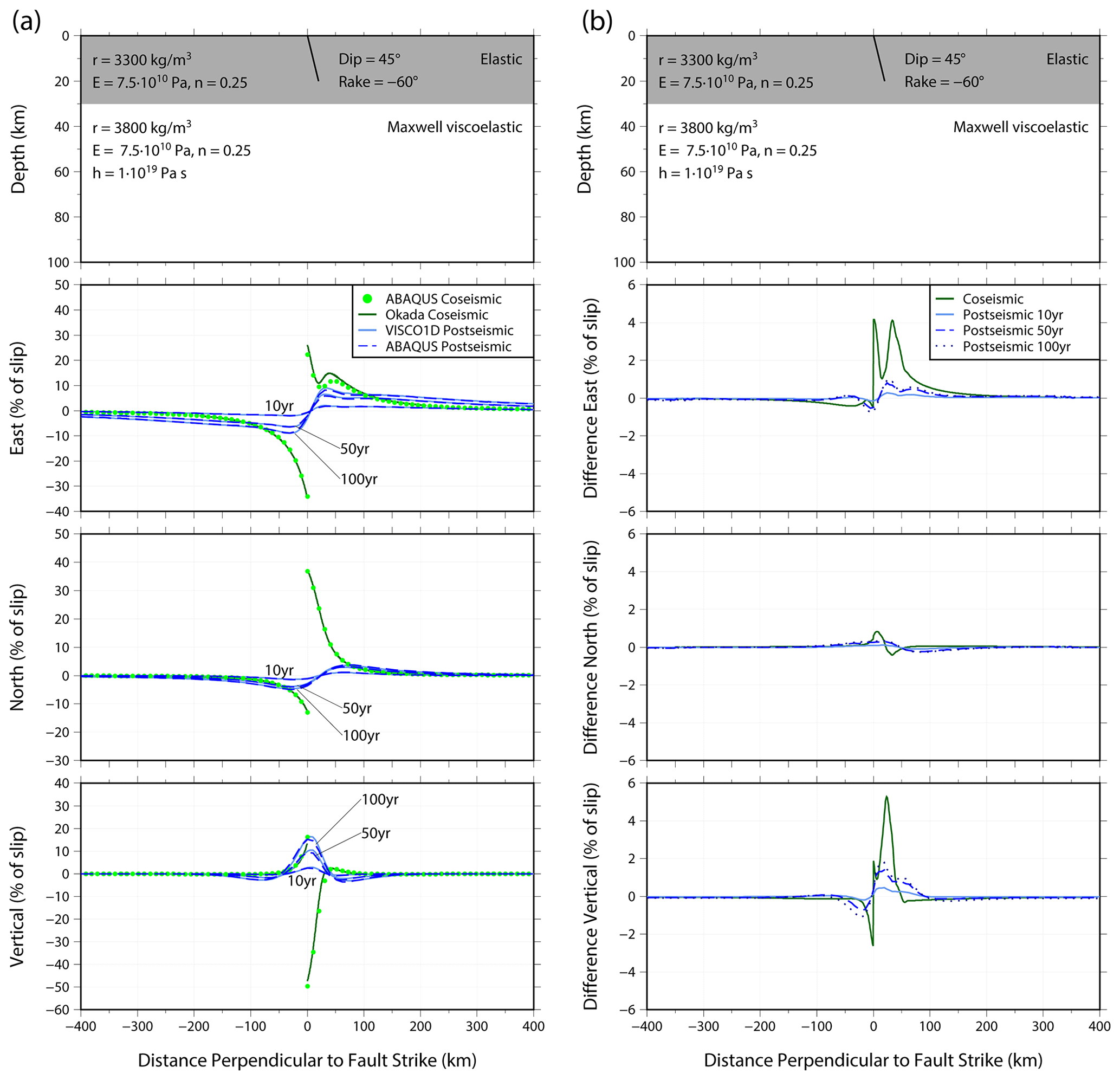
Figure 3Top panels of (a) and (b) show the fault dimensions and material properties of the upper 100 km of the model. Layers and material properties below 100 km depth are given in Table 2. (a) Coseismic (green) and post-seismic (blue) surface displacements in the east, north and vertical directions in response to slip on a strike-slip fault for a profile perpendicular to the fault strike. Results are calculated using the Okada analytical solution, VISCO1D and Abaqus (see legend). Post-seismic displacement is shown for times 10, 50, and 100 years after fault slip. Earth properties and fault dimension are given in top panel. Displacements are given as a percentage of the fault slip. (b) Differences between the Abaqus coseismic displacement and the Okada analytical solution (green) and the Abaqus post-seismic displacement and the VISCO1D displacement (blue). Differences are in terms of percentage of the fault slip.
4.1 Test setup
We perform three benchmarking tests each with different geometry: a strike-slip fault, a 30∘ dipping reverse fault and a 45∘ dipping fault with rake of −60∘, as summarised in Table 1. All faults outcrop at the surface of the model. The resolution of the mesh on the fault plane is 10×5 km. In plan view, the Abaqus mesh has 10 km elements in the vicinity of the fault, increasing to 50 km at the edge of the fault region, with elements in the surrounding low-resolution part, starting 1000 km away from the fault, being up to 500 km (Fig. 1). The element size increases with depth as shown in Table 2. For the 30∘ dipping reverse fault, we tested a coarser and a finer mesh and found that our chosen mesh resolution provided a satisfactory trade-off between computation time and accuracy, with the finer mesh giving only small differences in near- and far-field displacement compared to our chosen mesh, for a 10-fold increase in computation time. The results of this sensitivity test are discussed in more detail in Appendix A.
The model is run for 500 years to verify both the short- and long-term post-seismic deformation and for four iterations to ensure convergence of the self-gravitational solution. The Abaqus input files for the benchmarking tests are included in the supporting material (Nield, 2022). VISCO1D is run for the same time period and with maximum spherical harmonic degree of 2000, equivalent to ∼10 km resolution.
In all benchmarking tests, the same simple Earth structure is used (details for the Abaqus model are in Table 2), which is based on the Earth structure used by Pollitz (1997) for the uppermost 670 km, and we include a uniform lower mantle layer below. We found that the vertical deformation results for VISCO1D were sensitive to the number of layers in the input Earth structure and the presence of a lower mantle, so whilst the material properties are the same for both models, the VISCO1D Earth model contains more layers. We use this simple Earth structure to ensure our results are consistent with the Okada analytical solution for a homogenous half-space and the results presented by Pollitz (1997). We use a linear Maxwell rheology for all three benchmarking tests. We additionally verify the implementation of Burgers rheology against VISCO1D for the third test, with the transient viscosity (η) given in Table 2. Furthermore, we run the third test case in Abaqus using the elastic properties from PREM, keeping the same three-layer Maxwell viscosity profile as the benchmarking Earth model (Table 2). We do not benchmark the results from this test case as the Okada analytical solution is only valid for a homogeneous Earth. The input files for each test case and the Earth models used in the VISCO1D modelling for both Maxwell and Burgers rheology are given in the supporting material (Nield, 2022). All output displacements are shown normalised to the fault slip, in other words as a percentage of fault slip. This is consistent with the presentation of results by Pollitz (1997) and provides a useful metric for comparison of results. Differences between the model results are given as the difference between the percentages of fault slip.
4.2 Coseismic results
The results of the benchmarking exercises are shown in Figs. 3–5. We show coseismic displacement in the east, north and vertical directions for a profile perpendicular to the fault strike for each of the benchmarking tests. Surface displacement is shown in Appendix B, Figs. B1–B3. The Okada analytical solution is shown by the dark green line with the equivalent Abaqus coseismic output shown by the light green dots. The difference between the models is shown in panel (b) of Figs. 3–5. Overall, there is an excellent agreement between the Abaqus model and the Okada analytical solution. Of the three cases, the strike-slip fault agrees most closely (Fig. 3), with differences peaking at 1 % of the fault slip in the north direction (Fig. 3b). There are larger differences visible for the dipping fault cases (Figs. 4 and 5). Some of the near-field finer details of displacement in the east and vertical directions for the dipping faults (i.e. the directions with most displacement) are not perfectly captured by Abaqus, for example, at 50 km from the fault (see Fig. 4a, vertical direction), and we attribute this to the mesh resolution and the distorted element shape that is required to mesh around a dipping fault. However, these differences are a maximum of 6 % (Fig. 4b) and at distances greater than 300 km from the fault this decreases to less than 0.5 %. Since the aim of our model is to predict far-field deformation, these differences are acceptable.
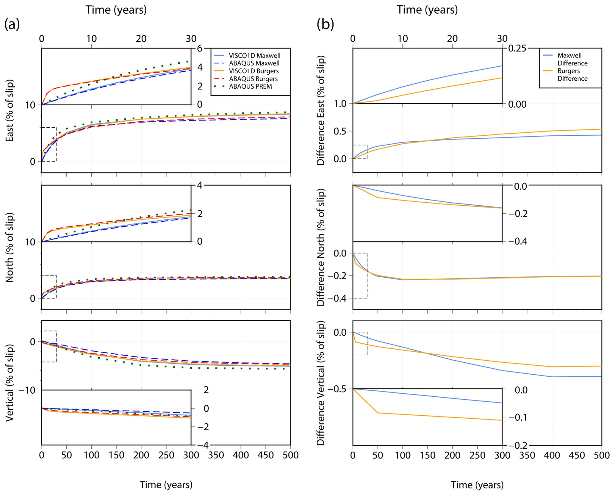
Figure 6(a) Post-seismic surface displacement through time in the east, north and vertical directions at a location 100 km perpendicular to the fault in Fig. 5. Predictions using two rheologies are shown: Maxwell rheology using VISCO1D and Abaqus; and Burgers rheology using VISCO1D and Abaqus (see legend). Predictions from Abaqus using the PREM elastic properties are also shown (green dots). The main plot for each displacement direction shows 500 years of displacement with the first 30 years shown in detail in the insets. Displacements are given as a percentage of the fault slip. (b) Difference between the Abaqus post-seismic displacement and the VISCO1D displacement for Maxwell rheology (light blue line) and Burgers rheology (orange line). Positive indicates Abaqus has less displacement than VISCO1D and negative indicates Abaqus has more displacement than VISCO1D. Differences are in terms of percentage of the fault slip. Note different scales on the y axis.
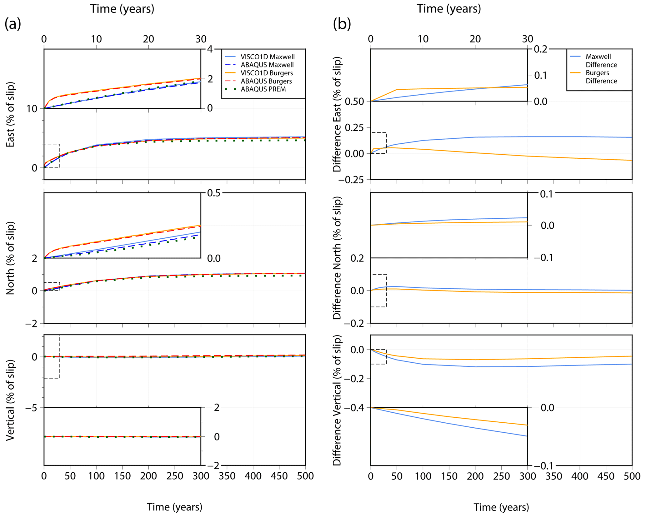
Figure 7As for Fig. 6 but for a location 300 km perpendicular to the fault in Fig. 5. Note different scales on the y axis.
4.3 Post-seismic results
Figures 3–5 also show profiles of the post-seismic displacement in the east, north and vertical directions for VISCO1D (light blue line) and the Abaqus model (dark blue dashed line). We show displacement as a percentage of fault slip at three times: 10, 50 and 100 years after the earthquake with corresponding differences between the models shown in panel (b) of each figure. Surface post-seismic displacement at each of these times is shown in Appendix B, Figs. B1–B3. The Abaqus predictions closely agree with VISCO1D for the strike-slip fault case (Fig. 3). Small differences can be observed for the dipping faults particularly in the vertical direction (Figs. 4b and 5b). The mismatch in the coseismic displacement due to limitations in mesh resolution is the cause of mismatch for the post-seismic displacement, i.e. less coseismic displacement from the Abaqus model would result in less stress and therefore less relaxation. Slight improvements in the near-field displacement could be made by increasing the mesh resolution in the vicinity of the fault but would come at a computational cost (see Appendix A). However, the differences remain small and are concentrated within 100 km of the fault with a maximum difference of 5 % of the fault slip after 100 years of relaxation (Fig. 4b) and less than 0.5 % at distances greater than 300 km from the fault. Therefore, we conclude that the model results are reliable for far-field post-seismic deformation.
Figures 6 and 7 show displacement through time for the fault geometry in test 3 for two points at 100 km (Fig. 6) and 300 km (Fig. 7) from the fault using both a Maxwell and Burgers rheology. There is clear consistency in the evolution of post-seismic relaxation between our model and VISCO1D, for both rheologies (compare solid with dashed lines in Figs. 6a and 7a). The insets in Figs. 6 and 7 show the results for the initial 30 years of the model run, where a rapid displacement can be observed from the transient viscosity of the Burgers rheology (orange/red lines) before converging with the results from the Maxwell model (blue lines) after approximately 30 years. Over the 500-year period, differences between our Abaqus model and VISCO1D for the Burgers rheology are less than 0.6 % of the fault slip within 100 km of the fault (Fig. 6b) or less than 0.1 % at distances of 300 km or more (Fig. 7b). For the Maxwell rheology, differences peak at 0.5 % of the fault slip within 100 km, reducing to 0.2 % at 300 km.
Figures 6a and 7a also show the displacement for test case 3 with the PREM elastic properties (green dotted lines). At 100 km distance from the fault (Fig. 6a), the different elastic structure results in slightly more coseismic displacement than the simple elastic structure used in the benchmarking tests, which results in greater post-seismic displacement with time. At 300 km distance from the fault (Fig. 7a), the depth-varying PREM elastic structure results in only very small differences. The surface coseismic and post-seismic displacements at 10, 50 and 100 years after the earthquake are shown in Fig. B4, Appendix B.
We have presented a finite-element model constructed in Abaqus for the purposes of modelling far-field coseismic and post-seismic deformation. The model is global, spherical and self-gravitating, and it allows for simple modification to include three-dimensional Earth structure, non-linear rheologies and alternative or multiple sources of stress change.
The model performs well when compared with the Okada coseismic analytical solution and predictions from the post-seismic VISCO1D programme for all three fault scenarios we have tested. For the coseismic displacement, differences are less than 6 % of the fault slip, with the largest differences in the vertical direction and near to the fault; in the fault far field, the differences are negligible. For the post-seismic displacement, differences are less than 5 % of the fault slip and at distances of 300 km from the fault, i.e. the far field which is the focus of our model, this reduces to differences of 0.5 %. Furthermore, we have verified that the evolution of displacement through time is an excellent match with VISCO1D for both Maxwell and Burgers rheologies. For interest, we also computed the displacement for test case 3 using the PREM elastic properties, finding differences in results within 100 km of the fault. However, in the far field, changing the elastic structure has minimal impact on the resulting post-seismic displacement as we used the same viscosity structure.
Inclusion of self-gravitation makes only a small difference for the displacement, peaking at 0.2 mm (less than 0.1 % of the fault slip) for the reverse fault (test 2) in the vertical displacement and is negligible in the horizontal directions. This demonstrates that it is not necessary to include self-gravitation when modelling post-seismic deformation in isolation, but it could become important when modelling post-seismic deformation alongside other larger sources of deformation such as changes in ice loading.
The main limitation of the model at present is that the geometry is restricted to a single fault plane within the mesh and it cannot have multiple segments of a fault plane with different strike or dip. This is due to the difficulties of constructing a valid spherical mesh in Abaqus with brick elements that conform to verification checks. For the same reason, including more than one earthquake in the same model would be problematic. This issue could potentially be resolved by employing external meshing software (e.g. Gmsh; Geuzaine and Remacle, 2009). In the case of a fault inversion that suggests multiple fault segments (e.g. Ye et al., 2014), an approximation of all the fault planes into a single geometry could still provide a realistic far-field estimate of post-seismic deformation (e.g. Takeuchi and Fialko, 2013), particularly if the fault geometry and slip are adjusted so that model output matches observations of coseismic displacement (e.g. Sun et al., 2018). Far-field post-seismic deformation is less sensitive to simplifications made to the fault geometry and slip distribution than near-field deformation (Khazaradze et al., 2002; Tregoning et al., 2013; Zhou et al., 2012). Alternatively, each fault segment could be analysed in a separate model and resulting deformation be combined, providing a linear rheology is used. The model can, however, account for varying slip and rake along the single fault plane by specifying individual values at each node pair. At present, the fault is not permitted to open, and whilst this is a realistic scenario for a fault, it would have negligible impact on the far-field post-seismic deformation.
We have demonstrated the validity of this model for far-field coseismic and post-seismic deformations. It is an improvement on existing models as it includes global spherical geometry, self-gravitation, and can be adapted to include 3-D Earth structure. It will prove particularly useful for investigating earthquakes in regions that may have large lateral variations in Earth properties where a 1-D Earth model cannot reproduce geodetic observations. Furthermore, the capability of Abaqus to model surface loading such as a changing ice load has already been established (e.g. van der Wal et al., 2010; Wu, 2004) and could easily be incorporated into this model.
In general, the higher the mesh resolution the more accurate the predictions of coseismic and post-seismic displacement. However, increases in the mesh resolution in the near field of the fault quickly result in a prohibitively large number of elements in the model, and it becomes computationally too expensive to run. To verify that our choice of mesh resolution is sufficient, we set up the 30∘ reverse fault test with a coarser and a finer mesh resolution and compared the model-predicted displacement in the near and far fields. Since the aim of our model is to calculate far-field post-seismic deformation, the convergence of displacement at distances of 300 km from the fault is what determines the choice of mesh resolution, although results are given for the near field for interest.
Table A1 shows the resolution of each mesh along with computation time for one iteration of the model. Note that this computation time is for parallel processing on eight cores on a standard Linux workstation. Due to the way Abaqus licensing works, individual setups may be faster than the time quoted in Table A1 if users have access to more cores and licenses. We term the mesh used in the main body of the paper the “reference mesh”.
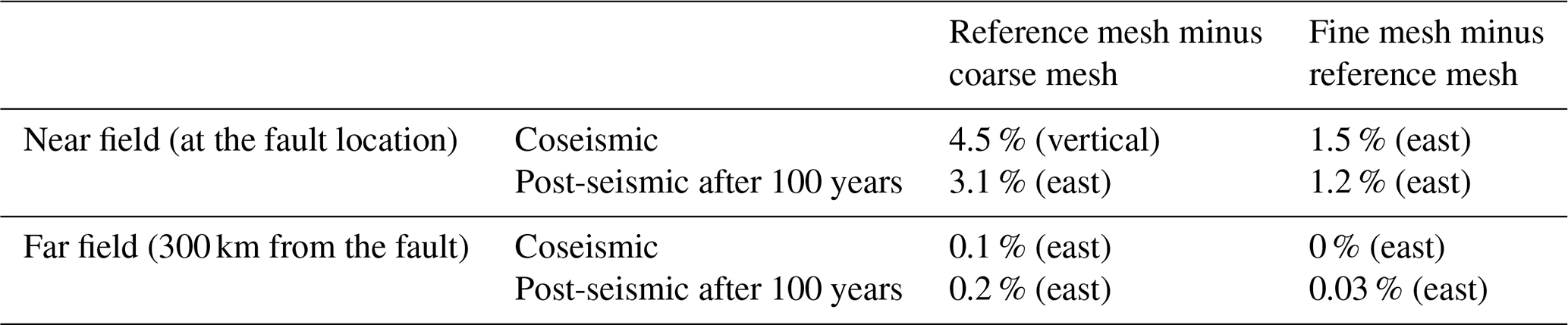
We evaluate overall displacement results in terms of differences in percentage of fault slip to be consistent with Figs. 3–7. The key results are summarised in Table A2. Comparing results for the reference mesh with the coarse mesh shows that near-field coseismic differences peak at 4.5 % of the fault slip and the maximum difference in the post-seismic deformation after 100 years is 3.1 %. When comparing the reference mesh with the fine mesh, this reduces to 1.5 % for coseismic differences and 1.2 % for post-seismic differences.
In the far field, however, differences between the coarse mesh and reference mesh are small, peaking at 0.2 % of the fault slip after 100 years of post-seismic deformation. Far-field differences between the reference mesh and the fine mesh are negligible. Since the focus of our model is the far field, these results might suggest that any of the mesh resolutions tested would be sufficient. However, in terms of absolute displacement, we see an improvement from differences of 5–9 mm between the coarse mesh and the reference mesh, and to 0.1–1.6 mm for differences between the reference and fine meshes. This demonstrates that results have converged at the resolution of our chosen mesh to be less than the magnitude of uncertainty associated with GPS-observed post-seismic deformation (e.g. Freed et al., 2006; Wang and Fialko, 2018). We therefore conclude that the chosen mesh resolution is more than fit for purpose, with only small improvements to near-field displacement to be gained by using a finer mesh.
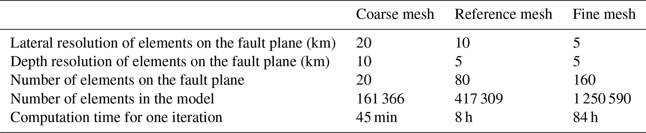
Table A2Differences in displacement (expressed as percentage of fault slip) between the different meshes in Table A1. In brackets is the direction of displacement where the maximum difference is observed.
This section shows surface displacement for the Abaqus model-predicted coseismic and post-seismic displacement for each of the three benchmarking tests with Maxwell rheology and for test case 3 using the elastic properties from PREM.
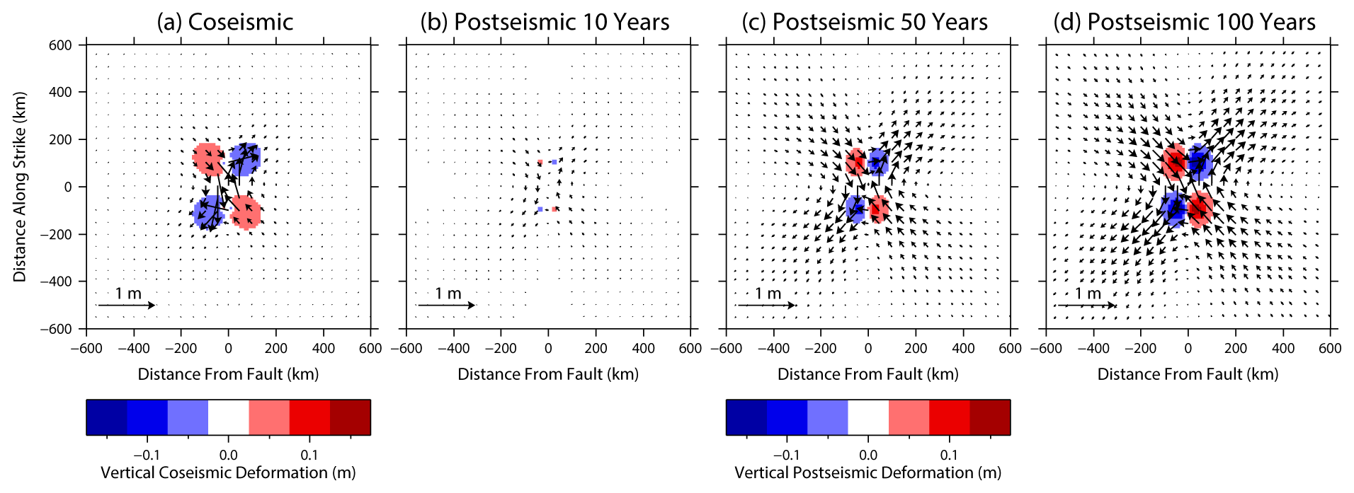
Figure B1Model-predicted surface displacement in response to slip on a strike-slip fault. Background colours show vertical displacement and arrows show horizontal displacement for (a) coseismic displacement; (b–d) post-seismic deformation at 10, 50, and 100 years after fault slip, respectively.
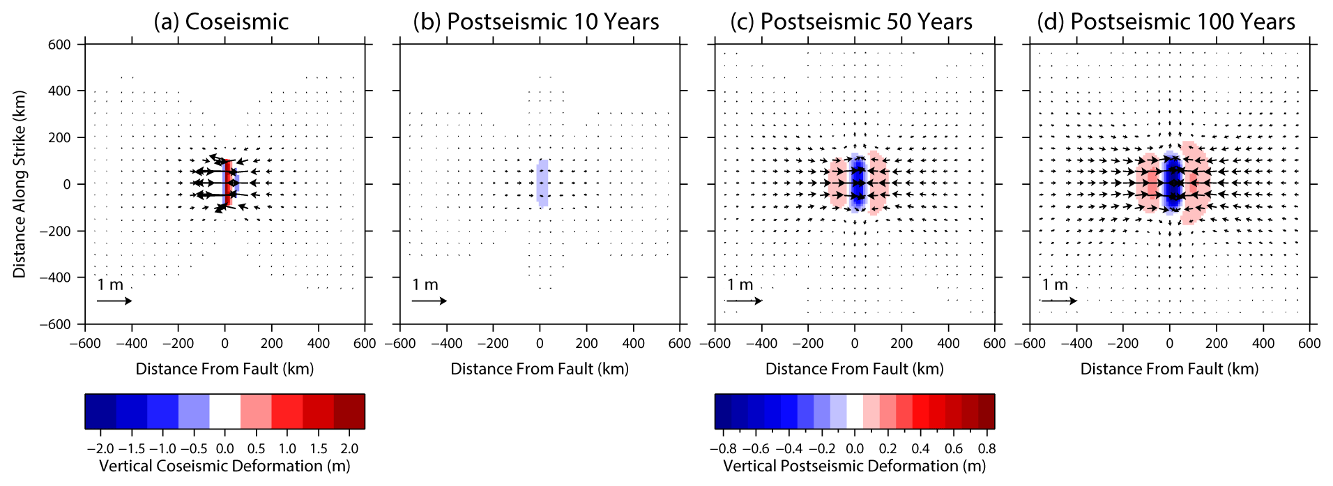
Figure B2As for Fig. B1 but for a 30∘ dipping reverse fault. Note the different colour scales for coseismic and post-seismic displacement.
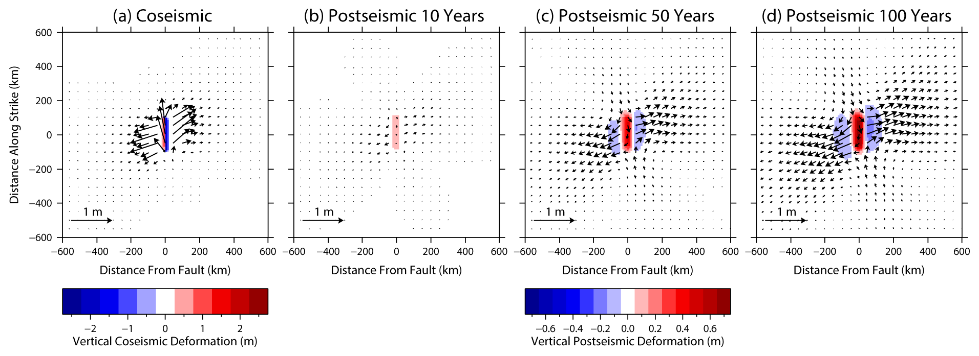
Figure B3As for Fig. B1 but for a 45∘ dipping fault. Note the different colour scales for coseismic and post-seismic displacement.
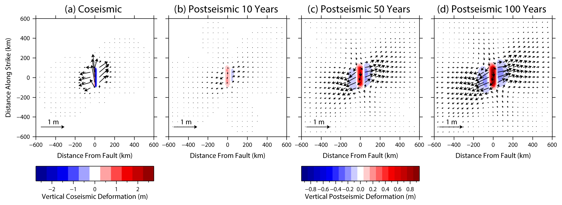
Figure B4As for Fig. B3, a 45∘ dipping fault, but using the PREM Earth model. Note the different colour scales for coseismic and post-seismic displacement.
Abaqus is a commercial software and can be purchased from the developer (https://www.3ds.com/products-services/simulia/products/abaqus/, last access: February 2019). We have used version 2018 in this study, but the methods and functionality used are available in older versions of the software as well. VISCO1D version 3 is available for download at https://www.usgs.gov/node/279413 (last access: March 2022; Pollitz, 2007).
Abaqus input files for all five models presented in this paper are available at https://github.com/ganield/ABAQUS_Postseismic_model/releases/tag/v2.0 (last access: 8 March 2022) and archived on Zenodo: https://doi.org/10.5281/zenodo.5897863 (Nield, 2022). Instructions on how to run the files are also available at this link. The VISCO1D input files and Earth model files used in the experiments presented in this paper are included in the GitHub repository, along with some instructions on how to run the code.
GAN developed the model. MAK conceived the study and consulted in the model implementation. RS contributed meshing code for Abaqus and consulted in the model development. BB contributed the self-gravitational part of the code. All authors contributed to the manuscript.
The contact author has declared that neither they nor their co-authors have any competing interests.
Publisher's note: Copernicus Publications remains neutral with regard to jurisdictional claims in published maps and institutional affiliations.
We are grateful to Fred Pollitz for making VISCO1D freely available and for his assistance with using the software. We also thank Tim Masterlark for his advice on implementing fault slip in Abaqus and Wouter van der Wal for guidance on constructing Abaqus models. The handling editor Lutz Gross and three anonymous reviewers are gratefully acknowledged for their constructive comments.
Grace A. Nield and Matt A. King are supported by the Australian Research Council Discovery Project (grant no. DP170100224).
This paper was edited by Lutz Gross and reviewed by three anonymous referees.
Agata, R., Barbot, S. D., Fujita, K., Hyodo, M., Iinuma, T., Nakata, R., Ichimura, T., and Hori, T.: Rapid mantle flow with power-law creep explains deformation after the 2011 Tohoku mega-quake, Nat. Commun., 10, 1385, https://doi.org/10.1038/s41467-019-08984-7, 2019.
Broerse, D. B. T., Vermeersen, L. L. A., Riva, R. E. M., and van der Wal, W.: Ocean contribution to co-seismic crustal deformation and geoid anomalies: Application to the 2004 December 26 Sumatra–Andaman earthquake, Earth Planet. Sci. Lett., 305, 341–349, https://doi.org/10.1016/j.epsl.2011.03.011, 2011.
Dziewonski, A. M. and Anderson, D. L.: Preliminary Reference Earth Model, Phys. Earth Planet. In., 25, 297–356, 1981.
Freed, A. M., Burgmann, R., Calais, E., and Freymueller, J.: Stress-dependent power-law flow in the upper mantle following the 2002 Denali, Alaska, earthquake, Earth Planet. Sc. Lett., 252, 481–489, https://doi.org/10.1016/j.epsl.2006.10.011, 2006.
Freed, A. M., Hirth, G., and Behn, M. D.: Using short-term postseismic displacements to infer the ambient deformation conditions of the upper mantle, J. Geophys. Res.-Sol. Earth, 117, B01409, https://doi.org/10.1029/2011jb008562, 2012.
Geuzaine, C. and Remacle, J.-F.: Gmsh: A 3-D finite element mesh generator with built-in pre- and post-processing facilities, Int. J. Numer. Methods Eng., 79, 1309–1331, https://doi.org/10.1002/nme.2579, 2009.
Han, S.-C., Sauber, J., and Pollitz, F.: Broadscale postseismic gravity change following the 2011 Tohoku-Oki earthquake and implication for deformation by viscoelastic relaxation and afterslip, Geophys. Res. Lett., 41, 5797–5805, https://doi.org/10.1002/2014gl060905, 2014.
Hayes, G. P.: The finite, kinematic rupture properties of great-sized earthquakes since 1990, Earth Planet. Sc. Lett., 468, 94–100, https://doi.org/10.1016/j.epsl.2017.04.003, 2017.
Hibbitt, D., Karlsson, B., and Sorenson, P.: Getting Started with ABAQUS – Version (6.14), Hibbitt, Karlsson & Sorensen, Inc., 2016.
Hirth, G. and Kohlstedt, D.: Rheology of the upper mantle and the mantle wedge: A view from the experimentalists, in: Inside the Subduction Factory, edited by: Eiler, J., Geophysical Monograph Series, AGU, 83–105, https://doi.org/10.1029/138GM06, 2003.
Hu, Y. and Wang, K.: Spherical-Earth finite element model of short-term postseismic deformation following the 2004 Sumatra earthquake, J. Geophys. Res.-Sol. Earth, 117, B05404, https://doi.org/10.1029/2012jb009153, 2012.
Hu, Y., Wang, K., He, J., Klotz, J., and Khazaradze, G.: Three-dimensional viscoelastic finite element model for postseismic deformation of the great 1960 Chile earthquake, J. Geophys. Res.-Sol. Earth, 109, B12, https://doi.org/10.1029/2004jb003163, 2004.
Huang, M.-H., Bürgmann, R., and Freed, A. M.: Probing the lithospheric rheology across the eastern margin of the Tibetan Plateau, Earth Planet. Sc. Lett., 396, 88–96, https://doi.org/10.1016/j.epsl.2014.04.003, 2014.
Karato, S. and Wu, P.: Rheology of the Upper Mantle – a Synthesis, Science, 260, 771–778, https://doi.org/10.1126/science.260.5109.771, 1993.
Khazaradze, G. and Klotz, J.: Short- and long-term effects of GPS measured crustal deformation rates along the south central Andes, J. Geophys. Res.-Sol. Earth, 108, 2289, https://doi.org/10.1029/2002jb001879, 2003.
Khazaradze, G., Wang, K., Klotz, J., Hu, Y., and He, J.: Prolonged post-seismic deformation of the 1960 great Chile earthquake and implications for mantle rheology, Geophys. Res. Lett., 29, 7-1–7-4, https://doi.org/10.1029/2002gl015986, 2002.
King, M. A. and Santamaría-Gómez, A.: Ongoing deformation of Antarctica following recent Great Earthquakes, Geophys. Res. Lett., 43, 1918–1927, https://doi.org/10.1002/2016gl067773, 2016.
Latychev, K., Mitrovica, J. X., Tromp, J., Tamisiea, M. E., Komatitsch, D., and Christara, C. C.: Glacial isostatic adjustment on 3-D Earth models: a finite-volume formulation, Geophys. J. Int., 161, 421–444, 2005.
Masterlark, T.: Finite element model predictions of static deformation from dislocation sources in a subduction zone: Sensitivities to homogeneous, isotropic, Poisson-solid, and half-space assumptions, J. Geophys. Res.-Sol. Earth, 108, 2540, https://doi.org/10.1029/2002jb002296, 2003.
Masterlark, T. and Wang, H. F.: Transient Stress-Coupling Between the 1992 Landers and 1999 Hector Mine, California, Earthquakes, B. Seismol. Soc. Am., 92, 1470–1486, 2002.
Masterlark, T., DeMets, C., Wang, H. F., Sánchez, O., and Stock, J.: Homogeneous vs heterogeneous subduction zone models: Coseismic and postseismic deformation, Geophys. Res. Lett., 28, 4047–4050, 2001.
Nield, G. A.: ganield/ABAQUS_Postseismic_model v2.0, Zenodo [data set], https://doi.org/10.5281/zenodo.5897863, 2022.
Okada, Y.: Surface deformation due to shear and tensile faults in a half-space, B. Seismol. Soc. Am., 75, 1135–1154, 1985.
Peña, C., Heidbach, O., Moreno, M., Bedford, J., Ziegler, M., Tassara, A., and Oncken, O.: Role of Lower Crust in the Postseismic Deformation of the 2010 Maule Earthquake: Insights from a Model with Power-Law Rheology, Pure Appl. Geophys., 176, 3913–3928, https://doi.org/10.1007/s00024-018-02090-3, 2019.
Pollitz, F. F.: Postseismic relaxation theory on the spherical earth, B. Seismol. Soc. Am., 82, 422–453, 1992.
Pollitz, F. F.: Gravitational viscoelastic postseismic relaxation on a layered spherical Earth, J. Geophys. Res.-Sol. Earth, 102, 17921–17941, https://doi.org/10.1029/97jb01277, 1997.
Pollitz, F. F.: Transient rheology of the upper mantle beneath central Alaska inferred from the crustal velocity field following the 2002 Denali earthquake, J. Geophys. Res.-Sol. Earth, 110, B08407, https://doi.org/10.1029/2005jb003672, 2005.
Pollitz, F. F.: VISCO1D-v3, USGS [code], https://www.usgs.gov/node/279413 (last access: March 2022), 2007.
Schmidt, P., Lund, B., and Hieronymus, C.: Implementation of the glacial rebound prestress advection correction in general-purpose finite element analysis software: Springs versus foundations, Comput. Geosci.-UK, 40, 97–106, https://doi.org/10.1016/j.cageo.2011.07.017, 2012.
Shao, Z., Zhan, W., Zhang, L., and Xu, J.: Analysis of the Far-Field Co-seismic and Post-seismic Responses Caused by the 2011 MW 9.0 Tohoku-Oki Earthquake, Pure Appl. Geophys., 173, 411–424, https://doi.org/10.1007/s00024-015-1131-9, 2016.
Steffen, R., Wu, P., Steffen, H., and Eaton, D. W.: On the implementation of faults in finite-element glacial isostatic adjustment models, Comput. Geosci.-UK, 62, 150–159, https://doi.org/10.1016/j.cageo.2013.06.012, 2014.
Suito, H. and Freymueller, J. T.: A viscoelastic and afterslip postseismic deformation model for the 1964 Alaska earthquake, J. Geophys. Res.-Sol. Earth, 114, B11404, https://doi.org/10.1029/2008jb005954, 2009.
Sun, T., Wang, K., and He, J.: Crustal Deformation Following Great Subduction Earthquakes Controlled by Earthquake Size and Mantle Rheology, J. Geophys. Res.-Sol. Earth, 123, 5323–5345, https://doi.org/10.1029/2017jb015242, 2018.
Takeuchi, C. S. and Fialko, Y.: On the effects of thermally weakened ductile shear zones on postseismic deformation, J. Geophys. Res.-Sol. Earth, 118, 6295–6310, https://doi.org/10.1002/2013jb010215, 2013.
Tregoning, P., Burgette, R., McClusky, S. C., Lejeune, S., Watson, C. S., and McQueen, H.: A decade of horizontal deformation from great earthquakes, J. Geophys. Res.-Sol. Earth, 118, 2371–2381, https://doi.org/10.1002/jgrb.50154, 2013.
van der Wal, W., Wu, P., Wang, H. S., and Sideris, M. G.: Sea levels and uplift rate from composite rheology in glacial isostatic adjustment modeling, J. Geodyn., 50, 38–48, https://doi.org/10.1016/j.jog.2010.01.006, 2010.
van der Wal, W., Whitehouse, P. L., and Schrama, E. J. O.: Effect of GIA models with 3D composite mantle viscosity on GRACE mass balance estimates for Antarctica, Earth Planet. Sc. Lett., 414, 134–143, 2015.
Wang, K. and Fialko, Y.: Observations and Modeling of Coseismic and Postseismic Deformation Due To the 2015 Mw 7.8 Gorkha (Nepal) Earthquake, J. Geophys. Res.-Sol. Earth, 123, 761–779, https://doi.org/10.1002/2017jb014620, 2018.
Wang, R., Lorenzo-Martín, F., and Roth, F.: PSGRN/PSCMP – a new code for calculating co- and post-seismic deformation, geoid and gravity changes based on the viscoelastic-gravitational dislocation theory, Comput. Geosci.-UK, 32, 527–541, https://doi.org/10.1016/j.cageo.2005.08.006, 2006.
Wu, P.: Using commercial finite element packages for the study of earth deformations, sea levels and the state of stress, Geophys. J. Int., 158, 401–408, https://doi.org/10.1111/j.1365-246X.2004.02338.x, 2004.
Wu, P., Wang, H. S., and Steffen, H.: The role of thermal effect on mantle seismic anomalies under Laurentia and Fennoscandia from observations of Glacial Isostatic Adjustment, Geophys. J. Int., 192, 7–17, https://doi.org/10.1093/gji/ggs009, 2013.
Ye, L., Lay, T., Koper, K. D., Smalley, R., Rivera, L., Bevis, M. G., Zakrajsek, A. F., and Teferle, F. N.: Complementary slip distributions of the August 4, 2003 Mw 7.6 and November 17, 2013 Mw 7.8 South Scotia Ridge earthquakes, Earth Planet. Sc. Lett., 401, 215–226, https://doi.org/10.1016/j.epsl.2014.06.007, 2014.
Zhong, S. J., Paulson, A., and Wahr, J.: Three-dimensional finite-element modelling of Earth's viscoelastic deformation: effects of lateral variations in lithospheric thickness, Geophys. J. Int., 155, 679–695, https://doi.org/10.1046/j.1365-246X.2003.02084.x, 2003.
Zhou, X., Sun, W., Zhao, B., Fu, G., Dong, J., and Nie, Z.: Geodetic observations detecting coseismic displacements and gravity changes caused by the Mw = 9.0 Tohoku-Oki earthquake, J. Geophys. Res.-Sol. Earth, 117, B05408, https://doi.org/10.1029/2011JB008849, 2012.
- Abstract
- Introduction
- Model setup
- Implementation of an earthquake
- Benchmarking
- Discussion and conclusions
- Appendix A: Mesh resolution test
- Appendix B: Surface displacement results
- Code availability
- Data availability
- Author contributions
- Competing interests
- Disclaimer
- Acknowledgements
- Financial support
- Review statement
- References