the Creative Commons Attribution 4.0 License.
the Creative Commons Attribution 4.0 License.
 | 21 Mar 2022
Novel coupled permafrost–forest model (LAVESI–CryoGrid v1.0) revealing the interplay between permafrost, vegetation, and climate across eastern Siberia
Simone M. Stuenzi
Julia Boike
Moritz Langer
Josias Gloy
Ulrike Herzschuh
Boreal forests of Siberia play a relevant role in the global carbon cycle. However, global warming threatens the existence of summergreen larch-dominated ecosystems, likely enabling a transition to evergreen tree taxa with deeper active layers. Complex permafrost–vegetation interactions make it uncertain whether these ecosystems could develop into a carbon source rather than continuing atmospheric carbon sequestration under global warming. Consequently, shedding light on the role of current and future active layer dynamics and the feedbacks with the apparent tree species is crucial to predict boreal forest transition dynamics and thus for aboveground forest biomass and carbon stock developments. Hence, we established a coupled model version amalgamating a one-dimensional permafrost multilayer forest land-surface model (CryoGrid) with LAVESI, an individual-based and spatially explicit forest model for larch species (Larix Mill.), extended for this study by including other relevant Siberian forest species and explicit terrain.
Following parameterization, we ran simulations with the coupled version to the near future to 2030 with a mild climate-warming scenario. We focus on three regions covering a gradient of summergreen forests in the east at Spasskaya Pad, mixed summergreen–evergreen forests close to Nyurba, and the warmest area at Lake Khamra in the southeast of Yakutia, Russia. Coupled simulations were run with the newly implemented boreal forest species and compared to runs allowing only one species at a time, as well as to simulations using just LAVESI. Results reveal that the coupled version corrects for overestimation of active layer thickness (ALT) and soil moisture, and large differences in established forests are simulated. We conclude that the coupled version can simulate the complex environment of eastern Siberia by reproducing vegetation patterns, making it an excellent tool to disentangle processes driving boreal forest dynamics.
- Article
(12691 KB) - Full-text XML
- BibTeX
- EndNote


Boreal forests cover vast areas of the Northern Hemisphere with strong gradients in climatic conditions and environments. They established in the Northern Hemisphere after the Last Glacial Maximum, leaving only a thin stretch in the north bordering the Arctic Ocean of pristine tundra areas (Mamet et al., 2019; Bonan, 2008; MacDonald et al., 2008). Anthropogenic climate warming is leading to the relaxation of warmth deficit limits at the northern margins and hence invasion of the tundra at a rate that is still unclear (Berner et al., 2013; Rees et al., 2020). At the same time, large parts of boreal forests, especially in eastern Siberia, are exposed to increasing disturbances (such as fires and drought), potentially driving a forest transition from deciduous species to evergreen taxa (Bonan, 2008; Herzschuh, 2020; Herzschuh et al., 2016). Accordingly, wildfires lead to increased greenhouse gas emissions through burning biomass and by deepening of the seasonally thawed layer for decades. The forest transition furthermore reduces the albedo, leading to a net positive global warming feedback, which will likely not be offset by increased carbon sequestration of a denser understorey vegetation (Bonan, 2008). However, the involved forest dynamics and interactions with the atmosphere and soil need to be considered in sufficient detail to forecast more realistic projections and to better understand the consequences for the boreal permafrost ecosystems of Siberia (Kirpotin et al., 2021).
Forest modelling is typically done globally, including the carbon cycle and permafrost, but individual trees and all life history stages need to be considered for a precise simulation. Modern global models such as LPJ-GUESS (Zhang et al., 2013) include individual models. The global models are used to show that forests will change and advance north. However, migration lags are typically not represented, and only climate envelopes serve for the distribution of plant functional types (PFTs). Dispersal processes and complexities have recently been recognized (Snell, 2014; Snell and Cowling, 2015; Lehsten et al., 2019) but are not yet used as standard for simulations. Furthermore, most modelling schemes still start with established trees, which makes them more general and computationally effective for a global application but at the cost of losing important detail for ecosystem responses (see discussion in Kruse et al., 2016). Also, the use of representative grid cells on a large grid without considering landscape will cause deviations to an extent that is unclear as to whether the impact on results is large and significant or not. Individual-based models (IBMs) could help here as they have sufficient detail of represented species and ecosystems, but applications are therefore only possible on landscapes not continents (Grimm and Railsback, 2005; DeAngelis and Mooij, 2005). Nevertheless, IBMs are the best tools to understand a system and develop general responses that can then inform or guide global model development. Further, neither a radiative transfer scheme through a multilayer canopy nor detailed representation of permafrost is included in typical simulation approaches.
Here, we aim at creating a model system that can accurately assess detailed thermal and hydrological fluxes between permafrost and forest cover as recently developed by Stuenzi et al. (2021a, b). The new model will include a dynamic vegetation model, which has a full life cycle to allow intraspecies and interspecies interactions at all stages (seed–seedling–mature tree), leading to nonlinear behaviour of population dynamics as well as resolving a three-dimensional landscape that is available for Siberian treeline areas developed by Kruse et al. (2016, 2019a, b).
We further developed two models and start each description by using the overview part of the ODD protocol for describing individual-based models (Grimm et al., 2010). We describe the host model LAVESI in Sect. 2.1, a spatially explicit, individual-based model handling the full life cycle of tree species and interactions among individuals and their environment. The second model, CryoGrid, which is informed by the host model and delivers improved state variables back to LAVESI, is described in Sect. 2.2: a one-dimensional, numerical land-surface model that simulates the thermo-hydrological regime of permafrost ground by numerically solving the heat conduction equation.
2.1 The 2D vegetation model LAVESI
2.1.1 Model description
The Larix vegetation simulator (LAVESI) is an individual-based spatially explicit model that simulates larch stand dynamics (Kruse et al., 2016, 2018). Monthly temperatures of the coldest (January) and warmest (July) months as well as precipitation series can force this model. In addition, 6-hourly data on wind speed and direction are needed to simulate seed distribution and tree reproduction, growth, and death (Kruse et al., 2019a, 2018, 2016). Recently the model has been extended by including topography and landscape sensing of the individuals (Sect. 2.1.2), and further boreal forest tree species were introduced aside from the larch species the model was initially developed for (Sect. 2.1.3; see full changes in Appendix A).
Purpose
The novel coupled model LAVESI–CryoGrid v1.0 was set up to understand tree stand structure, migration, and population dynamics of boreal forests growing between the leading edge at the Siberian treeline ecotone and the southern limit in response to a changing climate and its feedbacks with permafrost soils.
Table 1State variables of the model with dimensions and update rates ordered by the model's hierarchy levels. Based on the table provided in Kruse et al. (2016).
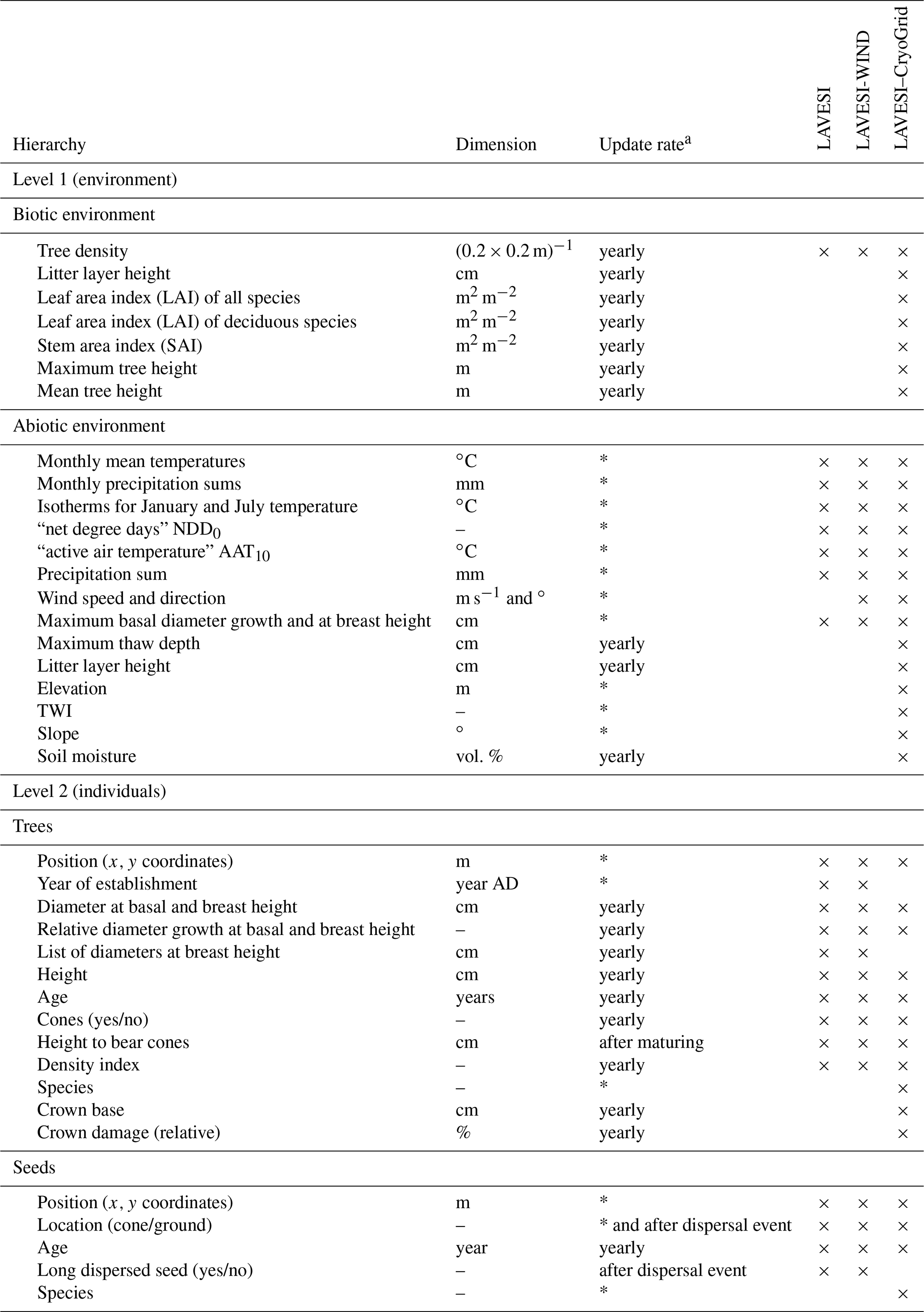
a Asterisks mean updated once at establishment (trees), production (seeds), or initialization (abiotic environment). NDD0 indicates the number of days exceeding 0 ∘C, and AAT10 is the sum of temperatures above 10 ∘C.
Entities, state variables, and scales
The model consists of two hierarchical levels characterized by a set of variables (Table 1): (1) simulation areas characterized by the specific biotic and abiotic environment and (2) individual trees and seeds.
The individual simulation areas are variable and have a size of typically 510×510 m (for parameterization and simulation experiments) on which seeds and trees are exactly positioned by x and y coordinates. Using the basal diameter of individual trees, the plot is overlaid with a tree density grid with a resolution of 0.2×0.2 m.
Simulation runs proceed in yearly time steps. We performed simulations for years 1–2100, prolonged by Representative Concentration Pathway (RCP) prediction scenarios. Additionally, to reach stabilization of population dynamics and the forcing climate series, simulations were preceded by a stabilization period with a length of 1000 years (for parameterization and sensitivity analysis). All simulations start from bare ground introducing 5000 ha−1 yr−1 seeds in the first 50 years, and to allow for repopulation of simulation areas after extinction, 100 ha−1 yr−1 seeds are added every year to the simulation areas.
Process overview and scheduling
The simulation proceeds in yearly time steps from the beginning to the end of the input climate time series, which includes a stabilization period to ensure that emerging populations reach equilibrium with the environment. In each initialization phase of each simulation run, the weather data are processed and used to estimate maximum diameter growth (at basal and breast height) for each simulation year based on 10-year mean climate auxiliary variables (see details in Sect. 2.2.2 “Description of sub-models” in Kruse et al., 2016). Within the growth processes of the model, these variables are used to individually estimate the current diameter growth of trees constrained by their actual biotic (competition) and abiotic (landscape features: elevation, TWI, slope, soil moisture, active layer depth) environment (design concept: sensing). Stochasticity in the model was introduced by using random numbers generated with a pseudo-random number generator (mt19937_64, from the random library) to allow for different results between two or more consecutive runs of the model (design concept: stochasticity).
Within 1 simulation year, the following processes become consecutively invoked (see Fig. 2 in Kruse et al., 2016; detailed explanations for each process can be found in a corresponding section in 2.2.2 “Description of sub-models”). Update of environment. Interactions between neighbouring trees are local and indirect. Basal diameters of each individual tree are used to evaluate the competition strength. We use a yearly updated density map to pass information about competition for resources between trees (design concept: interaction). Further, a litter layer and the state variables of each grid cell are updated as well. Growth. The individual growth of basal diameter and, if a tree reached a height of 1.3 m, of breast height diameter is calculated from the maximum possible growth in the current year affected by the tree's density index and its abiotic environment. From the resulting diameters, the tree height is estimated differently for two height classes: smaller and greater than 1.3 m (design concept: collectives). Seed dispersal. Seeds in “cones” are dispersed from the parent trees at a set rate. The dispersal directions and distances are randomly determined from a ballistic flight influenced by wind speed and direction with decreasing probabilities for long distances and only to places lower than the release height. If dispersed seeds leave the extent of the simulated plot they are removed from the system, but optionally they could be introduced from the other side or only on the east–west margins, depending on the user's choice. Seed production. Trees produce seeds after the year at which they reached their stochastically estimated maturation height. The total amount depends on weather, competition, and tree size. Optionally, the pollen donor for the pollination of ovules of seeds produced can be selected by a wind-determined and distance-dependent probability distribution function using a von Mises distribution. Establishment. The seeds that lie on the ground germinate at a rate depending on current weather conditions and is constrained by the actual litter layer height. Mortality. Individual trees or seeds die, i.e. they become removed from the plot, at a specified mortality rate. For trees this is deduced from long-term mean weather values, a drought index, surrounding tree density, and tree age and size, plus a background mortality rate. Seeds, on the other hand, have the same constant mortality rate whether on trees and or the ground (design concept: emergence). Ageing. Finally, the age of seeds and trees increases once a year, and seeds are removed from the system when they reach a defined species age limit.
2.1.2 Addition of landscape sensing
Data from the digital elevation model (DEM) TanDEM-X 90 m were downloaded from the web service provided by the German Aerospace Center (DLR https://download.geoservice.dlr.de/TDM90/, last access: 31 July 2021; Krieger et al., 2007). Subsequently, the tiles were reprojected to the corresponding Universal Transverse Mercator (UTM) zone of the focus areas (Khamra N49, Nyurba N50, Spasskaya Pad N52). All tiles were merged for each subzone and resampled by linear interpolation from 90 to 30 m resolution using functions from the “raster” package in R (Hijmans, 2020). The results were imported in SAGA GIS version 2.3.2 (Conrad et al., 2015) and subjected to a basic terrain analysis tool using the standard parameters. The resulting rasters were water-masked using the cloud-based geospatial data analysis platform Google Earth Engine (GEE, Gorelick et al., 2017) to assess Sentinel-2 imagery between 1 May and 15 October 2018 with a cloud cover of less than 20 % and thresholds manually set for spectral band B12 (2190 nm) until all water was masked out by comparing them to true-colour satellite images. The DEM along with slope angle and terrain water index (TWI, moisture content) were cropped to 510×510 m (260 100 m2) areas for this study and exported as plain text files for import into LAVESI.
LAVESI reads these data provided in 30 m resolution and interpolates linearly from the closest four grid cells for each 20 cm grid tile of the environment grid. Based on empirical relationships of forest presence for combinations of slope angle and TWI established in a study by Shevtsova et al. (2021), an environment growth impact factor (Envirgrowth, 0–1) is calculated for each tile, and tree diameter growth at this position is reduced accordingly (Eq. 1, Appendix B):
where TWIi is the interpolated terrain water index of the 20×20 cm2 environmental grid cell i, and Slopei is the slope angle of the same grid cell i.
Seed dispersal has been improved. Seeds can now only be dispersed to places which are at the same elevation as or a lower elevation than the release height in the terrain.
Table 2Species traits and model variable values in LAVESI either newly introduced for this study, adjusted from the initial version LAVESI v1.01 (*), or introduced in the predecessor LAVESI-WIND v1.0 (**). Values from * Abaimov et al. (1998), ** Sato et al. (2016), own analyses, educated guess, or parameter fitting.

2.1.3 Addition of species and estimating leaf area index (LAI)
Further species were added to the existing model presented in Kruse et al. (2016). To add a fast forward implementation of species in LAVESI, we modified the code so that the programme can be started with either one or all species in a mix simultaneously. The species are numbered (integer values), which are used internally to assess species-related variables (Table 2) when called for in the functions as necessary. Therefore, the code is independent from the species and allows adding species or functional types simply by adding a new line in the new specieslist.csv in the main folder of LAVESI.
For this study, we analysed field data from the Chukotka and central Yakutia 2018 expedition in the same way as we did for Chukotka (Biskaborn et al., 2019; Kruse et al., 2019b). In the area of central Yakutia, species belonging to the Pinaceae family form the forests. From these, two deciduous boreal forest tree species were sampled, Larix cajanderi Mayr. (LACA) and Larix gmelinii (Rupr.) Rupr., (LAGM), as were three evergreen species, Picea obovata Ledeb. (PIOB), Pinus sibirica Du Tour (PISI), and Pinus sylvestris L. (PISY) (Kruse et al., 2019b). While the two larch species are best adjusted to the harsh environment of northeastern Siberia and are able to grow on shallow active layers above permafrost, they differ mainly in their frost hardiness, and the species LACA can even endure colder temperatures in winter (Table 2). PIOB is a competitor for L. gmelinii growing at similar environmental conditions but preferring deeper thawed active layers of a minimum of 200 cm. On well-drained sites, PISY grows well and outcompetes the other species. In milder environments, LASI and PISI grow on similar sites as LAGM and PIOB.
Tree-ring width data were established from tree discs and cores collected from sites close to Lake Khamra and from the region Nyurba. The discs and tree cores were prepared by standard dendroecological processing steps: (1) sanding with progressively finer paper until tree rings are clearly visible, (2) making high-resolution images for a track with a binocular and attached camera, (3) detecting rings with CooRecorder (Cybis Elektronik & Data AB) and cross-dating, and (4) exporting individual tree-ring chronologies (more details in Kruse et al., 2020). Tree-ring width data per species were then imported to R using the dplR package (Bunn et al., 2020), and regression models were set up by fitting nonlinear functions using generalized least squares with the gnls function from the nlme package (Pinheiro et al., 2019). For each species, we extracted the median of the loess-smoothed (span: 1.5) yearly growth increase of individual trees and set up a generalized least squares regression using a nonlinear model. This was successful for LACA, LAGM, and PIOB, but not for PISI and PISY due to small sample sizes, for which current values of PIOB are used as a first estimate (Table 2). For each tree in the simulation, the maximum actual growth can be estimated with the following equation:
where TRW is the tree-ring width for species i at 1 year depending on the fitted parameters gdbasalconst, gdbasalfac, and gdbasalfacq.
Biomass data were prepared following the protocol of Shevtsova et al. (2020), and allometric relationships were established to empirically estimate the leaf area (LA) from total leaf biomass for each tree (Eq. 3), followed by a log–log linear regression forced to pass through the origin employing the basal diameter as an explanatory variable (Eq. 4). To estimate the LA for each tree, we used specific leaf area (SLA) parameters to translate from the dry weight of needles to leaf area (Eq. 3). For each species, the SLA was extracted from literature values: SLALAGM=120 cm2 g−1 (Xian-Kui et al., 2015), which was also used for the closely related sister species LACA, SLAPIOB=50 cm2 g−1 (Konôpková et al., 2020), and SLAPISY=50 cm2 g−1 (extracted from the most recent source Błasiak et al., 2021, although other values are reported; 34 cm2 g−1 in Reich et al., 1998, 40 cm2 g−1 in Mencuccini and Bonosi, 2001). For PISI no source for SLA values was found and we assume it is similar to PISY:
where BM is the biomass of tree i in grams, and SLA is the specific leaf area for species j.
Here, a is the slope of the linear model fit and DB is the basal diameter of the tree i for species j.
During simulations runs with LAVESI, the LA for each individual tree is estimated based on the fitted linear regression model using the following equation.
The leaf area index (LAI) of each CryoGrid 10×10 m grid cell in LAVESI is then the sum of leaf area values of present trees. When a tree crown area covers more than one cell, the value is distance-weighted on the closest grid cells. For each species, the crown radius is estimated from field data with a log–log linear regression, and the slope and y intercept are used in LAVESI: parameters crownradiusestslope and crownradiusestinterc, respectively (Table 2).
2.1.4 Addition of a dynamic litter layer and estimating active layer thickness (ALT)
A dynamic, growing litter layer with constant growth of 0.5 cm yr−1 and stochastic disturbance effects was introduced in the Environmentupdate function of LAVESI. When the parameter litterlayer is switched on, each of the 20 cm grid cells have a chance that the litterlayerheight can be reduced. This is stochastically implemented and for each year there is a 10 % chance the litter layer is reduced by 10 %, a 9 % chance of a 25 % reduction, a 0.9 % chance of 50 %, a 0.09 % chance of 90 %, and a 0.01 % chance of a 99 % reduction. This leads to a litter layer of ∼15 cm in the areas of interest in simulation runs, as observed in the region of interest (Kruse et al., 2019b). With this functionality, locally acting insulation effects are included in the estimation of the actual ALT in one environment grid cell. The estimation of the maximum active layer thickness was already introduced in the original setup of LAVESI (Kruse et al., 2016) and still serves as a first estimate, thus making it possible to run a stand-alone simulation of LAVESI without coupling to the CryoGrid (see below).
2.1.5 Model validation
We compared results from simulations until the year 2015 with field inventories from the 2018 expedition and literature values, focusing on the following key regions: Lake Khamra (westernmost, warmest), Nyurba (intermediate, climate station), and Spasskaya Pad (easternmost for boreal forests of Yakutia) for which we used literature values for comparison. Values were in the range of expected results.
2.2 The 1D permafrost model CryoGrid
2.2.1 Model description
The model used to simulate the thermo-hydrological interactions between permafrost ground and the forest canopy is based on CryoGrid (originally described in Westermann et al., 2016). CryoGrid is a one-dimensional, numerical land-surface model that simulates the thermo-hydrological regime of permafrost ground by numerically solving the heat conduction equation. The CryoGrid model has recently been extended by a multilayer canopy module developed by Bonan et al. (2014) for use in boreal permafrost regions (see Stuenzi et al., 2021a, b, for model details). The multilayer canopy model provides a comprehensive parameterization of fluxes from the ground through the canopy layer up to a roughness sublayer. In combination with CryoGrid the canopy model replaces the standard surface energy balance scheme, while soil state variables are passed back to the forest module. Following Stuenzi et al. (2021b), a realistic canopy structure is simulated by allowing fractional compositions of deciduous and evergreen taxa within a simulated forest stand.
Purpose
The model CryoGrid-Vegetation (Stuenzi et al., 2021a) was set up to understand the heat and water exchange between the atmosphere, boreal forest, and permafrost. The coupled multilayer vegetation–permafrost model reproduces the energy transfer and thermal regime of typical boreal permafrost ecosystems at different study sites in boreal permafrost regions.
Entities, state variables, and scales
Model entities are multiple layers of atmosphere and vegetation (based on Bonan, 2008), as well as permafrost (based on CryoGrid, Westermann et al., 2016). The physically based, numerical land-surface model simulates the radiative heat and water transfer through the atmosphere, vegetation, and ground at a 1D scale.
The simulation proceeds at a 5 min time step. The numerical model simulates the aboveground and belowground temperature field based on temporally changing conditions at the ground surface and top of the canopy–atmosphere boundaries.
Process overview and scheduling
To simulate the thermo-hydrological regime of the permafrost ground CryoGrid solves the one-dimensional heat equation numerically including groundwater phase change. The canopy model was coupled to CryoGrid by replacing its standard surface energy balance scheme, while soil state variables are passed back to the forest module. The vegetation module forms the upper boundary layer of the model and provides a comprehensive parameterization of fluxes from the ground through the canopy up to the roughness sublayer. This allows the simulation of diverse forest canopy structures and their impact on the vertical moisture and energy transfer. The exchange of radiation, sensible heat, condensation, and evaporation at the different layers are simulated with a surface energy balance scheme based on atmospheric stability functions. In every time step top-of-the-canopy incoming radiation and precipitation are partitioned at each layer throughout the canopy. The change of internal energy in the subsurface domain (ground) over time is composed of fluxes across the upper (surface energy balance below the canopy) and lower (geothermal heat flux at 100 m depth, 0.05 W m−2) boundaries. The model simulates the evolution of the snow cover based on an extensive CROCUS-based snowpack scheme (Zweigel et al., 2021). Furthermore, rainfall and snowfall are intercepted throughout the canopy with only a fraction reaching the ground directly as throughfall. The remaining water and/or snow is added to the canopy layers as canopy water and/or snow, which either evaporates or reaches the ground as canopy drip or stem flow in the following time steps. The model is forced by standard meteorological variables, which can be obtained from automatic weather stations, reanalysis products, or climate models. The required forcing data include air temperature, precipitation (solid and liquid), wind speed, incoming shortwave and longwave radiation, humidity, and air pressure (Westermann et al., 2016).
2.2.2 Model validation and parameters
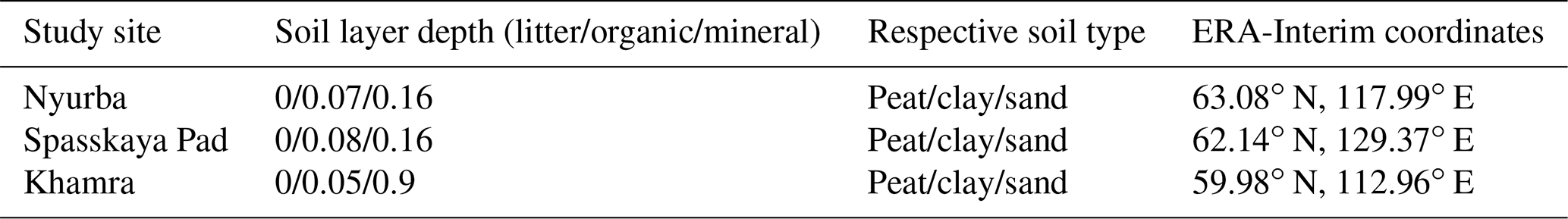
This entire model setup has previously been extensively validated for different study sites throughout our study region, including Nyurba (63.08∘ N, 117.99∘ E), Spasskaya Pad (62.14∘ N, 129.37∘ E), and Ilirney (67.40∘ N, 168.37∘ E) (Stuenzi et al., 2021a, b). Validation exercises were carried out based on measured and modelled ground surface temperature (GST), active layer thickness (ALT), soil moisture, Bowen ratio, and shortwave and longwave radiation below and above the canopy. Parameters defining the canopy, snow, and soil properties were set according to literature values, model documentation, and own measurements (see Stuenzi et al., 2021b, for constants and multilayer canopy parameter choices). Table 3 summarizes the parameter choices for the three different sites. Appendix C, Table C1 summarizes the commonly used CryoGrid parameters.
2.3 Coupling the models
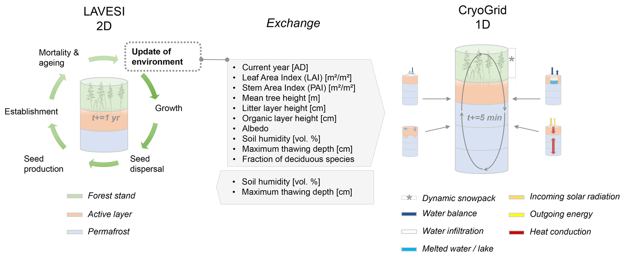
The coupled model setup benefits from the detailed process implementation gained while developing the individual models and brings the 1D to a landscape simulation. Therefore, we can reproduce the energy transfer and thermal regime in permafrost ground as well as the radiation budget, nitrogen and photosynthetic profiles, canopy turbulence, and leaf fluxes, while at the same time predicting the expected establishment, die-off, and treeline movements of larch forests (Fig. 2). In our analyses, we focus on vegetation and permafrost dynamics and reveal the magnitudes of different feedback processes between permafrost, vegetation, and current and future climate in Siberia.
LAVESI serves as host model and can now be set to call individual CryoGrid instances in a given year. For this, the data in LAVESI are aggregated on a 10×10 m grid superimposed on the 20×20 cm grid. Key state variables are leaf area index (LAI), stem area index (SAI), fraction of deciduous species, litter layer height, organic layer height, albedo, and the soil moisture in percent (plant-available water, PAW), which are provided to CryoGrid. These values can either be sorted by LAI and exported for five quartiles (implemented but not used here) or from the three areas that are equal slices from left to right (used here, see Appendix B). When the output file is created, LAVESI can be set to either start CryoGrid directly via a system call or schedule the instance with a bash file for the workload manager slurm (Yoo et al., 2003). Based on the key state variables provided by LAVESI for each of the areas, CryoGrid starts three (or five) parallel simulations. Once the output has been written, LAVESI reads the file and produces for the three levels anomalies for available soil water and active layer thickness. With these anomalies, the 10×10 m CryoGrid grid in LAVESI is filled and, from this, the anomalies used to calculate the new values for each 20×20 cm environment grid cell. When the quartile mode is set, the state values are assigned to this grid calculated by linear interpolation of the LAI-sorted state values and anomalies are calculated as in the other mode.
The multilayer canopy model in CryoGrid requires a minimum LAI of 0.7 m2 m−2 and a minimum height of 1 m to successfully build the radiative transfer scheme from the atmosphere to the ground; therefore, forest cover below these values is ignored.

Figure 1Scheme of focus areas covered on the Chukotka and central Yakutia 2018 expedition. Region II: boreal forest bi-stability summergreen–evergreen transition needed for the expansion of species in addition to Larix cajanderi and L. sibirica. Data in map: treeline (Walker et al., 2005); ESA CCI Land Cover forest classes (ESA, 2017).
2.4 Forcing data and landscape of focus areas
The meteorological forcing data required by the multilayer canopy-permafrost model (air temperature, air pressure, wind speed, relative humidity, solid and liquid precipitation, incoming longwave and shortwave radiation, and cloud cover) are obtained from ERA-5 (ECMWF Reanalysis, Hersbach et al., 2020). The data are extracted for the focus regions Nyurba (63.08∘ N, 117.99∘ E; covering sites EN18067, EN180-68, EN180-70), Spasskaya Pad (62.14∘ N, 129.37∘ E), and Lake Khamra (59.97∘ N, 112.96∘ E; covering EN18079–83; Fig. 1).
To provide a millennia-long time series for model spin-up of LAVESI these series were matched to historical climate data for the forcing retrieved from the 0.5∘ × 0.5∘ Climate Research Unit gridded Time Series (CRU TS version 3.23) monthly data (1901–2014) (Harris et al., 2020). By repeating the 20th century data in a loop, a 2100-year-long monthly climate series was established from 1 to 2100 CE for each focus region using the RCP2.6 prediction scenario.
2.5 Simulation experiments
We forced LAVESI simulations with the RCP2.6 climate scenario by calling CryoGrid first in 2015 and yearly in the following years, letting the simulation run until the year 2030. Simulation runs were started with the updated LAVESI version on an empty landscape with true topography starting at 1 CE to allow for spin-up and ending in 2100 CE. Into the empty landscape, seeds (5000 ha−1 yr−1) for initiating population establishment were introduced for the first 50 years. Subsequently, only 100 ha−1 yr−1 seeds were introduced to allow for re-establishment after a complete die-out of trees on the whole simulation area. Each simulation was rerun without calling CryoGrid to compare the differences when the improved active layer thickness and available soil water are used.
In addition to the simulation that uses equal proportions of seeds of each species introduced into the simulation area, we started individual simulations for each single species.
2.6 Statistical analyses
All statistical analyses in this study were performed in R 3.6.1 (R Core Team, 2019) and mostly using included standard functions, with the addition of functions from the package “lattice” (Sarkar, 2008) for plotting the data.
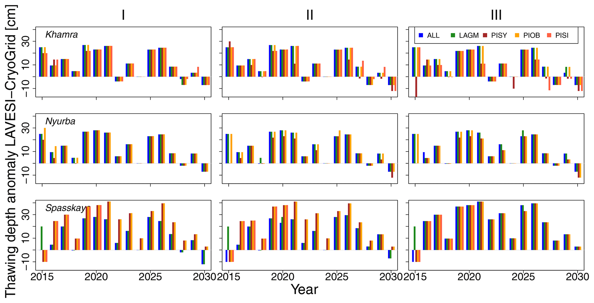
Figure 3Thawing depth anomaly in the coupled simulation model for all focus areas (rows) and areas within the simulation areas (columns: I, II, and III) for year steps 2015–2030. LAGM: Larix gmelinii; PIOB: Picea obovata; PISI: Pinus sibirica; PISY: Pinus sylvestris.

Figure 4Soil moisture anomalies in the coupled simulation model for all focus areas (rows) and areas within the simulation areas (columns: I, II, and III) for year steps 2015–2030. LAGM: Larix gmelinii; PIOB: Picea obovata; PISI: Pinus sibirica; PISY: Pinus sylvestris.
3.1 Simulations results with LAVESI
A gradient of population densities (expressed in LAI values) forms, which negatively follows the TWI gradient on all sites (I: left, driest to III: right, wettest, Figs. 5–7, Appendix E, Fig. E1). Further, an increase in larch dominance towards nearly pure larch tree stands can be observed from Khamra (southwest, warmest) via Nyurba (intermediate) to Spasskaya Pad (northeast, coldest). Stand densities are highest in the mixed-species simulations at Nyurba (∼1.9 m2 m−2), larger than at the warmers site Khamra (∼1.5 m2 m−2), and lowest at Spasskaya (0.9 m2 m−2). Regarding other species, PISY is present in mixed stands in small numbers and grows only in open stands in simulations with only this species, suggesting that this species prefers a certain environment (Appendix B and D). PIOB performs better in single monospecific runs, leading to larger LAI than in mixed stands, but also reaches dense populations in warm areas (Khamra) and has the smallest sizes at coldest sites (Spasskaya Pad, Figs. 5–7). LAGM grows under most conditions but not in the wettest areas (highest TWI values, Appendix D).
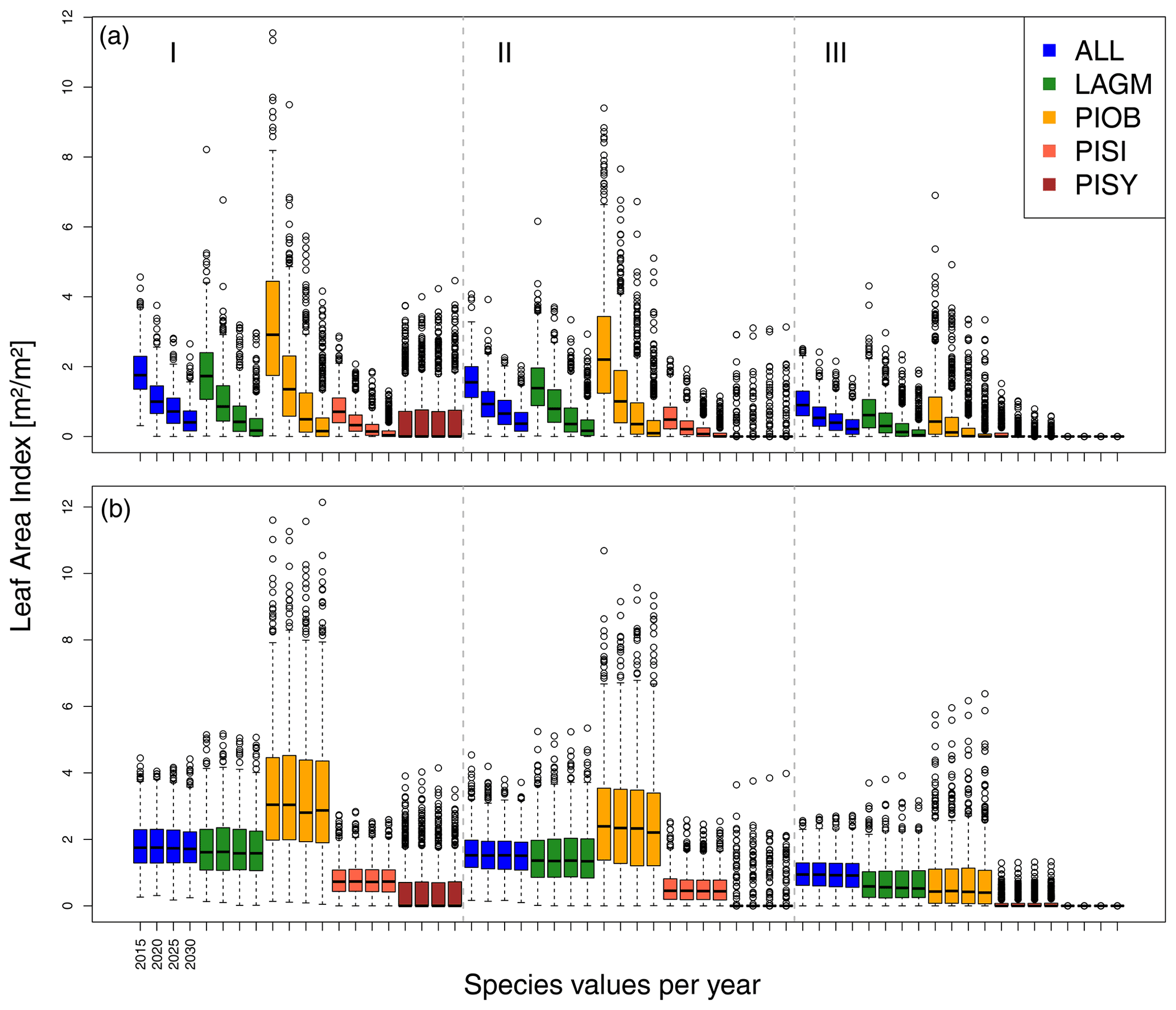
Figure 5Leaf area index (LAI) values at Lake Khamra for the three areas within the simulation areas (I, II, III) on the same plot at which CryoGrid was called (upper row) and only LAVESI runs (lower row). LAGM: Larix gmelinii; PIOB: Picea obovata; PISI: Pinus sibirica; PISY: Pinus sylvestris.
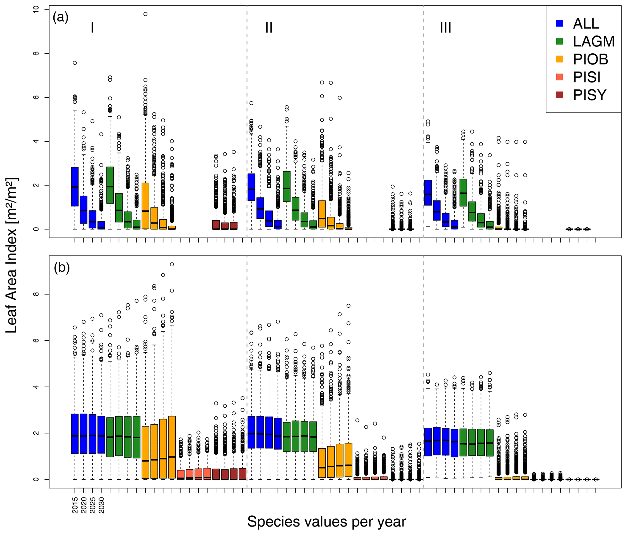
Figure 6Leaf area index (LAI) values at Nyurba for three areas within the simulation areas (I, II, III) on the same plot at which CryoGrid was called (upper row) and only LAVESI runs (lower row). LAGM: Larix gmelinii; PIOB: Picea obovata; PISI: Pinus sibirica; PISY: Pinus sylvestris.
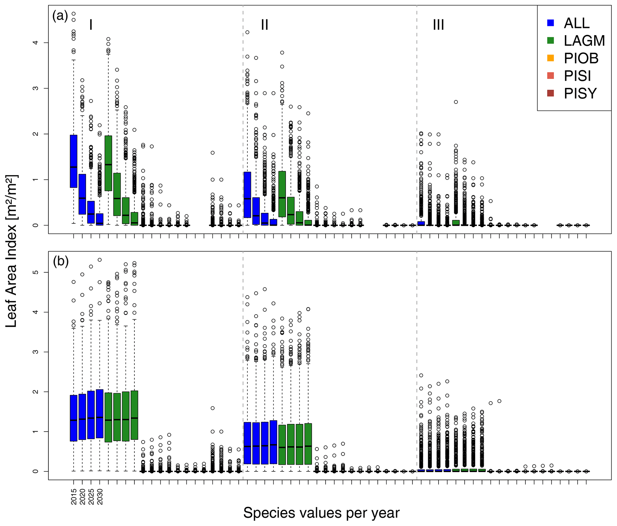
Figure 7Leaf area index (LAI) values at Spasskaya Pad for three areas within the simulation areas (I, II, III) on the same plot at which CryoGrid was called (upper row) and only LAVESI runs (lower row). LAGM: Larix gmelinii; PIOB: Picea obovata; PISI: Pinus sibirica; PISY: Pinus sylvestris.
3.2 Comparing simulations with LAVESI and the coupled version
The values are very similar for the runs with all and individual species. In nearly all years, LAVESI's ALT values are higher by up to 20 cm (mean over all is 109.6±11.4 cm versus 96.1±10.2 cm, which is ∼14.1 %) at all focus regions (Fig. 3). The soil moisture anomaly fluctuates around 0 % at Lake Khamra, is lower in the coupled model for Nyurba by ∼10 %, and lower at Spasskaya Pad by ∼20 % than in simulations using only LAVESI (Fig. 4).
Smaller population sizes can be observed in all simulations, leading to a drop in LAI values when LAVESI is updated by CryoGrid (comparing lower to upper panels in Figs. 5–7). In CryoGrid coupled runs, species grow with less dense stands but still cover the same area. In the coupled runs, populations die out in some cases at the end of the simulation at year 2030 (Appendix D).
Table 4Qualitative comparison of simulation results to expectations based on observations.
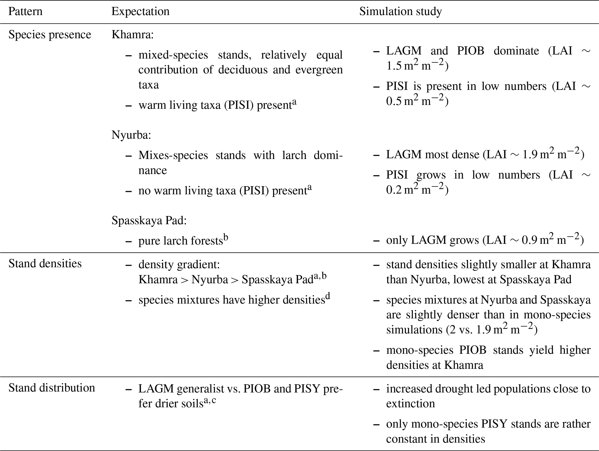
a Kruse et al. (2019b); b Ohta et al. (2001), Sugimoto et al. (2002); c Mamet et al. (2019); d Liang et al. (2016).
4.1 Simulation performance
Species preference matches observations and expectations (Table 4, Kuznetsova et al., 2010). Larches have a wide ecological niche and are widespread (Mamet et al., 2019). They are generalists and best adapted to the harsh Siberian environments that were predominantly wet but have now become drier with global warming (Churakova et al., 2021; Kharuk et al., 2021). Picea obovata grows best in the westernmost warm areas and reaches larger LAI and biomass than when growing in mixed stands competing with other species (Kharuk et al., 2007). This is as expected, and competition, as Wieczorek et al. (2017) show, seems to be a strong factor dampening the response of tree stands when climatic conditions improve. Further, the simulation of denser stands at the Khamra site contradicts the general observation that mixed-species stands are more productive and/or denser than the niches occupied (Liang et al., 2016), but depending on the stand structure it could be negative (Zeller et al., 2018) and is in line with the observation of Chen et al. (2003).
4.2 The coupled version LAVESI–CryoGrid
The simulations using site information for the three focus sites yield dense tree stands in LAVESI simulations but not in the coupled version. The coupled model results in smaller key soil parameters, active layer thickness (ALT), and plant-available water (PAW). PAW has a strong impact as trees grow poorly in conditions exceeding drought and waterlogging thresholds (e.g. Liang et al., 2014; Mamet et al., 2019; Lawrence et al., 2015; Barber et al., 2000). Drought leads to a higher mortality of trees, and in consequence, population simulations are driven close to extinction within the simulation duration of 15 years. However, when drought-adapted Pinus sylvestris occupies the niche, there is nearly no change and it could, in the end, colonize the simulation areas. This matches expectations and further implies that the model is reproducing the natural dynamics well (Table 4).
As fires become more intense and frequent under global warming, spruce or other species may become dominant rather than shade-intolerant larch species. In the currently naturally deciduous, larch-covered areas, evergreen taxa may invade and change the heat fluxes and energy balance with the threat of entering a positive feedback loop such as a deepening of the ALT (Bonan, 2008; Stocker et al., 2013; Stuenzi et al., 2021b).
In general, technical issues arise when coupling models and implementing I/O indirectly via output files. The two different time steps (years in LAVESI vs. 5 min in CryoGrid) and computational speeds lead to long computation times and high requirements of computational resources for the coupled version. To avoid any delay, a parallelization of CryoGrid simulations, as implemented here, is highly recommended, especially for dry study sites where a simulated year in CryoGrid can take up to 4 h. We find that simulations of homogeneous areas perform best, especially when the exchange is set up using three to five instances sorted by LAI. The constraint lies here and more instances would improve the representation of variants of deciduous- and/or evergreen-covered plots, but these improved LAVESI simulations come at the cost of computation time when not using the parallelized version as developed for this study.
The as-is application of LAVESI overestimates ALT values by around 14 %, and therefore we advise using the implemented correction from CryoGrid for forecasting forest dynamics in the proposed coupled version. The 3D simulations provide a way to understand permafrost distribution and interactions with vegetation. Further implementations, tracked online in the GitHub repository of LAVESI, include spatially explicit fire and trait variation and adaptation. This public sharing of the source code plus advances in both models allows easy exchange, development, and adaptation to further regions. This and the simple setup make the coupled model version easy to implement and thus offers wide applicability. However, fieldwork or literature values for present species and stand structure as well as soil moisture and temperature time series from remote areas are necessary to adjust parameters and adapt the model and species to local site conditions, which is an issue for the vast remote areas in Siberia. With increasing data from these remote areas, such as better satellite imagery coverage and resolution, the collection of more detailed field data (loggers recording soil temperatures and moisture in the active layer), and monitoring of permafrost dynamics and tree growth, the drivers of forest dynamics may be disentangled and thus improve the model.
Table A1Complete ODD “overview” table for LAVESI. Improvements from left to right; normal text represents unchanged model parts, while bold font highlights novel developments.
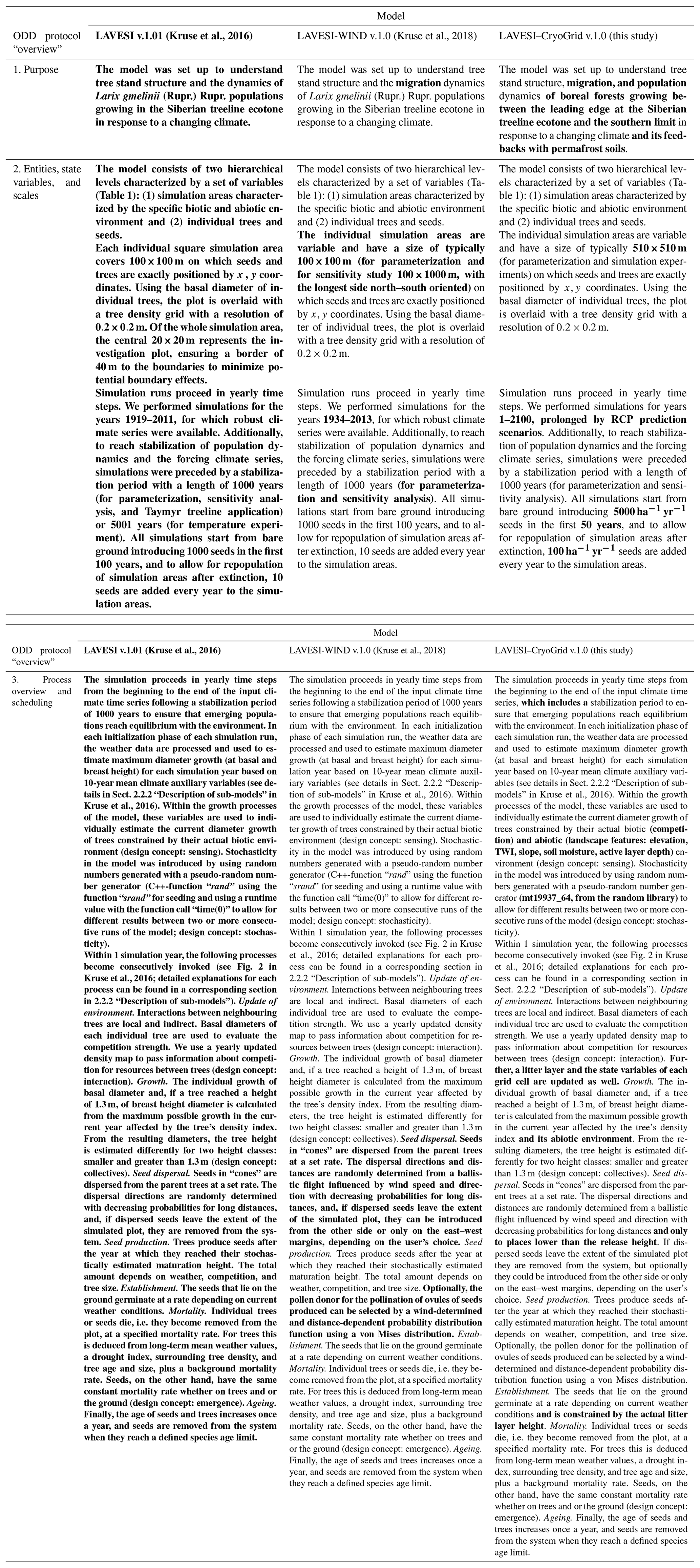
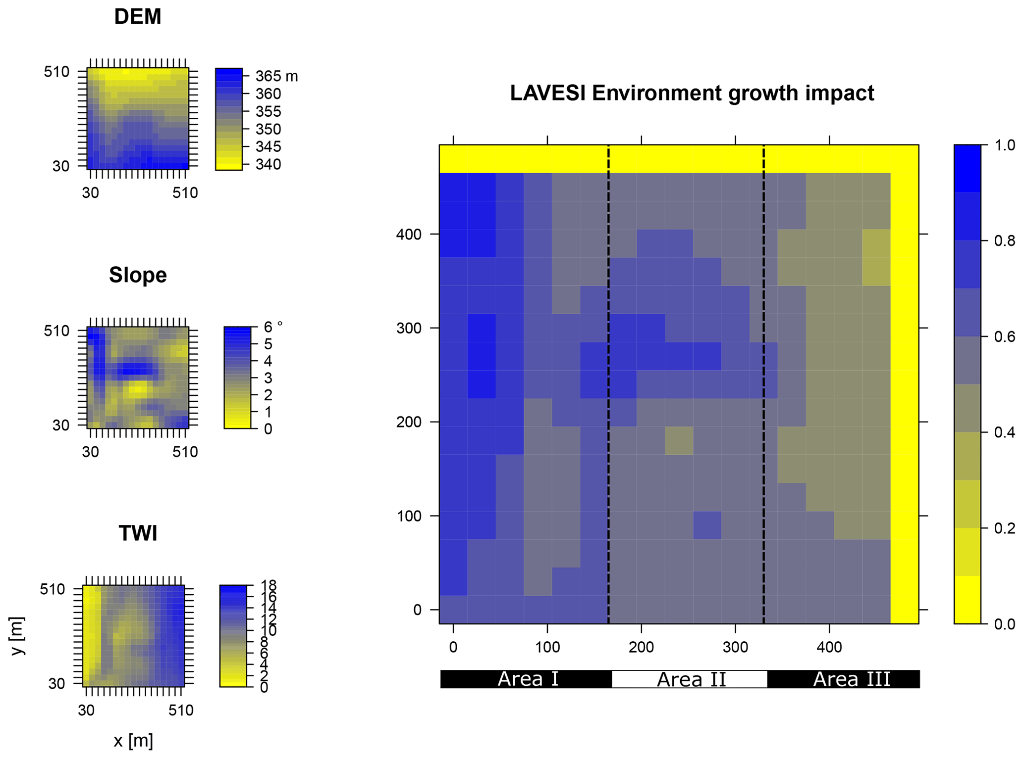
Figure B1Elevation (DEM), slope angle, and terrain water index (TWI) define the environment growth impact (0 no growth possible; 1 good, no constraints) using an empirically fitted function for present forest growth at the area of interest Khamra.
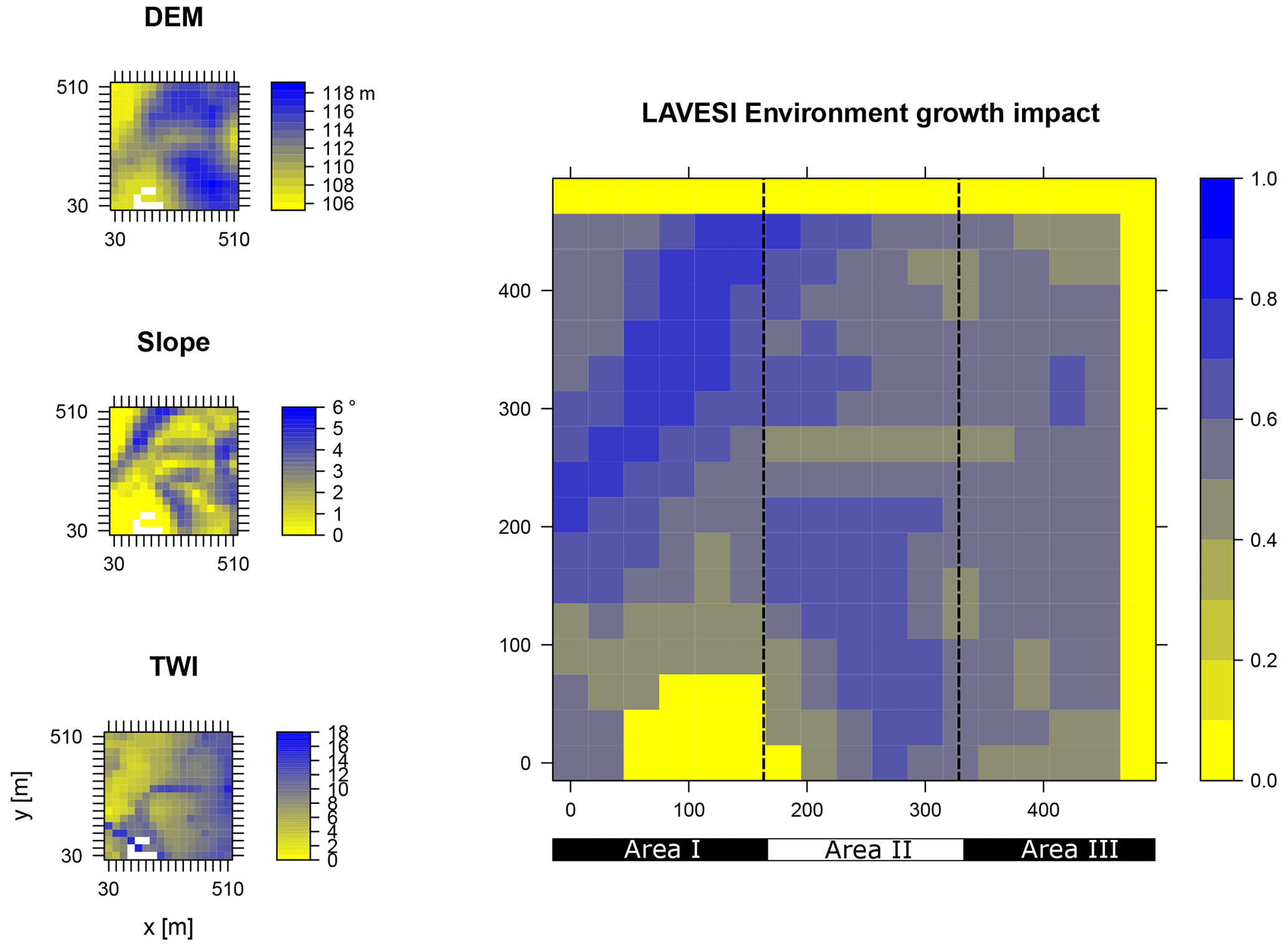
Figure B2Elevation (DEM), slope angle, and terrain water index (TWI) define the environment growth impact (0 no growth possible; 1 good, no constraints) using an empirically fitted function for present forest growth at the area of interest Nyurba.
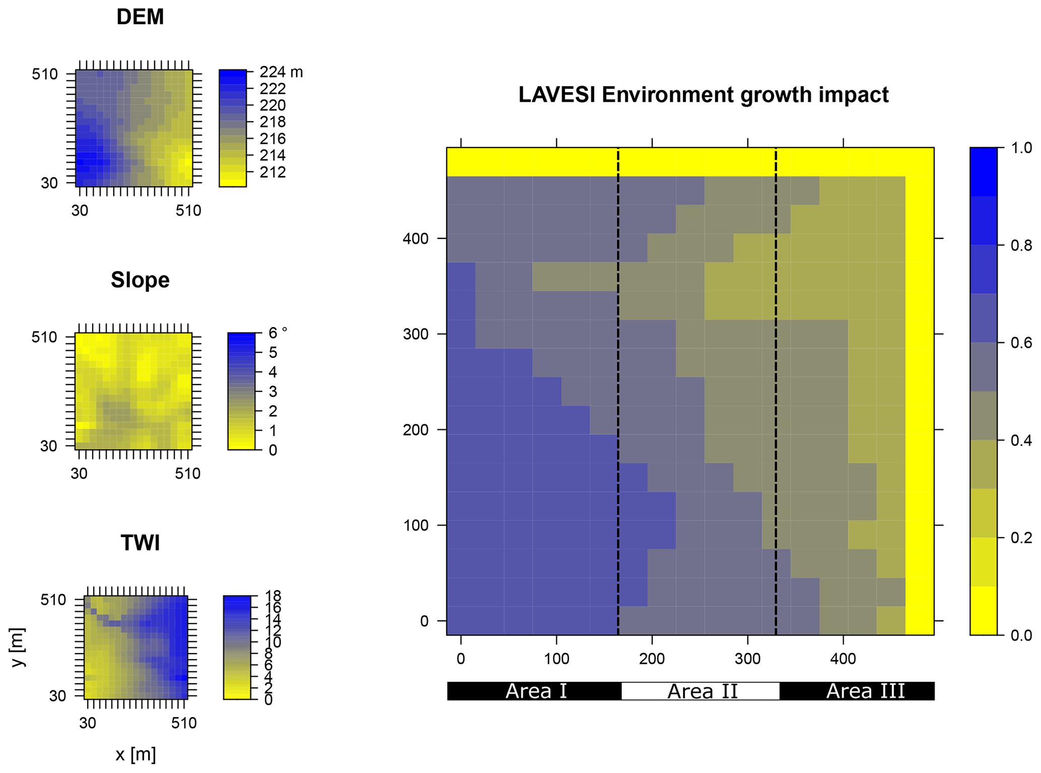
Figure B3Elevation (DEM), slope angle, and terrain water index (TWI) define the environment growth impact (0 no growth possible; 1 good, no constraints) using an empirically fitted function for present forest growth at the area of interest Spasskaya Pad.
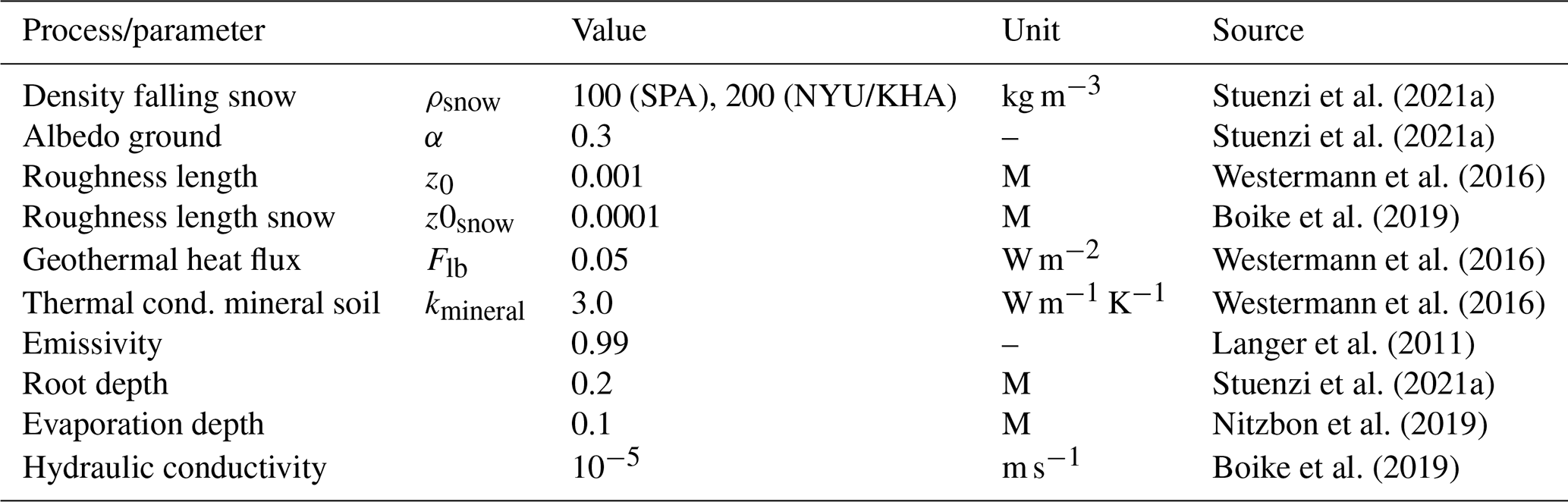
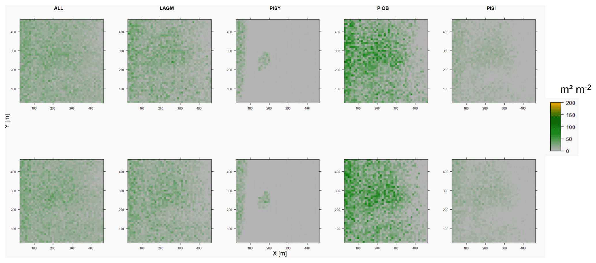
Figure D1Leaf area index (LAI) values of the CryoGrid grid aggregated at year 2015 at Lake Khamra. Upper row shows LAVESI–CryoGrid coupled; lower row shows LAVESI simulations. LAGM: Larix gmelinii; PIOB: Picea obovata; PISI: Pinus sibirica; PISY: Pinus sylvestris.

Figure D2Leaf area index (LAI) values of the CryoGrid grid aggregated at year 2020 at Lake Khamra. Upper row shows LAVESI–CryoGrid coupled; lower row shows LAVESI simulations. LAGM: Larix gmelinii; PIOB: Picea obovata; PISI: Pinus sibirica; PISY: Pinus sylvestris.

Figure D3Leaf area index (LAI) values of the CryoGrid grid aggregated at year 2025 at Lake Khamra. Upper row shows LAVESI–CryoGrid coupled; lower row shows LAVESI simulations. LAGM: Larix gmelinii; PIOB: Picea obovata; PISI: Pinus sibirica; PISY: Pinus sylvestris.

Figure D4Leaf area index (LAI) values of the CryoGrid grid aggregated at year 2030 at Lake Khamra. Upper row shows LAVESI–CryoGrid coupled; lower row shows LAVESI simulations. LAGM: Larix gmelinii; PIOB: Picea obovata; PISI: Pinus sibirica; PISY: Pinus sylvestris.
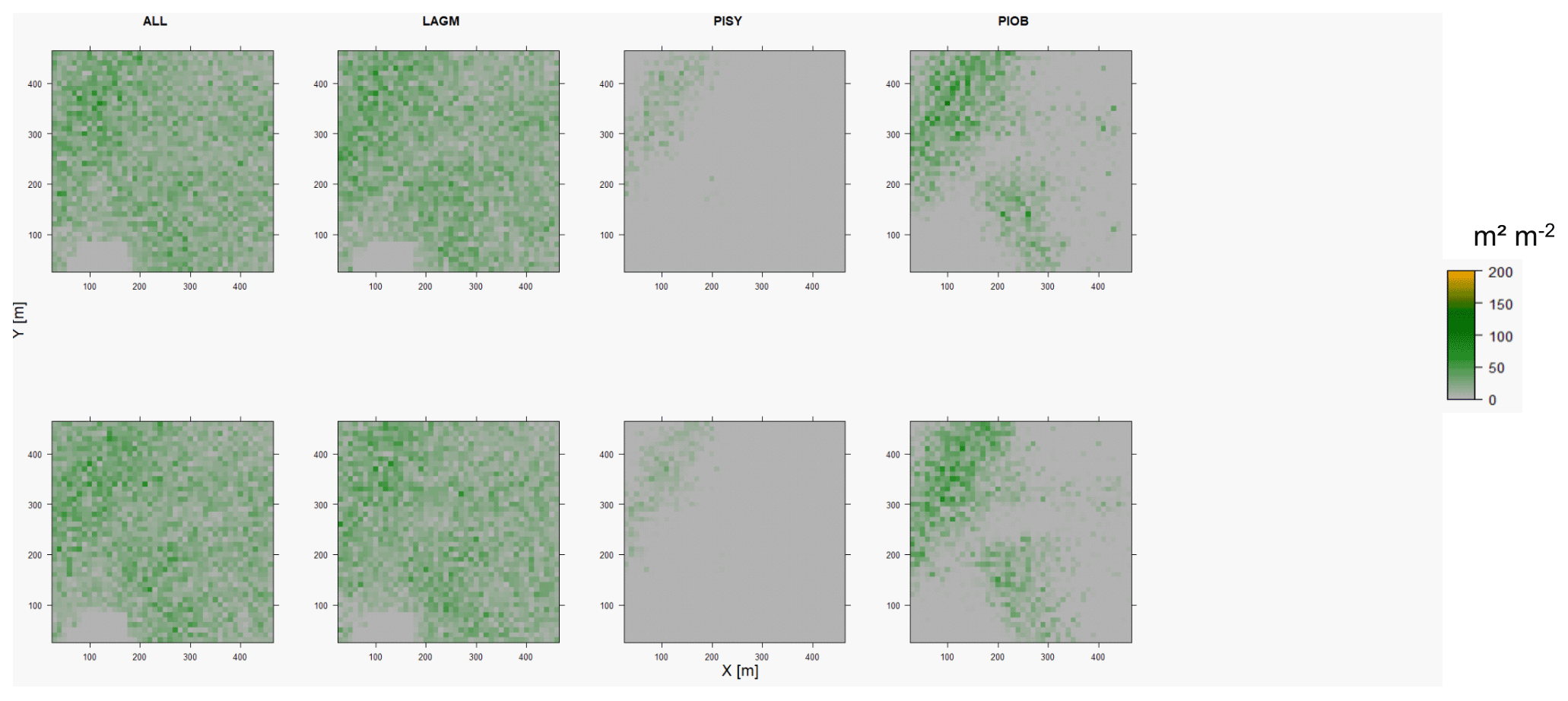
Figure D5Leaf area index (LAI) values of the CryoGrid grid aggregated at year 2015 at Nyurba. Upper row shows LAVESI–CryoGrid coupled; lower row shows LAVESI simulations. LAGM: Larix gmelinii; PIOB: Picea obovata; PISI: Pinus sibirica; PISY: Pinus sylvestris. Simulations with PISI were not possible.
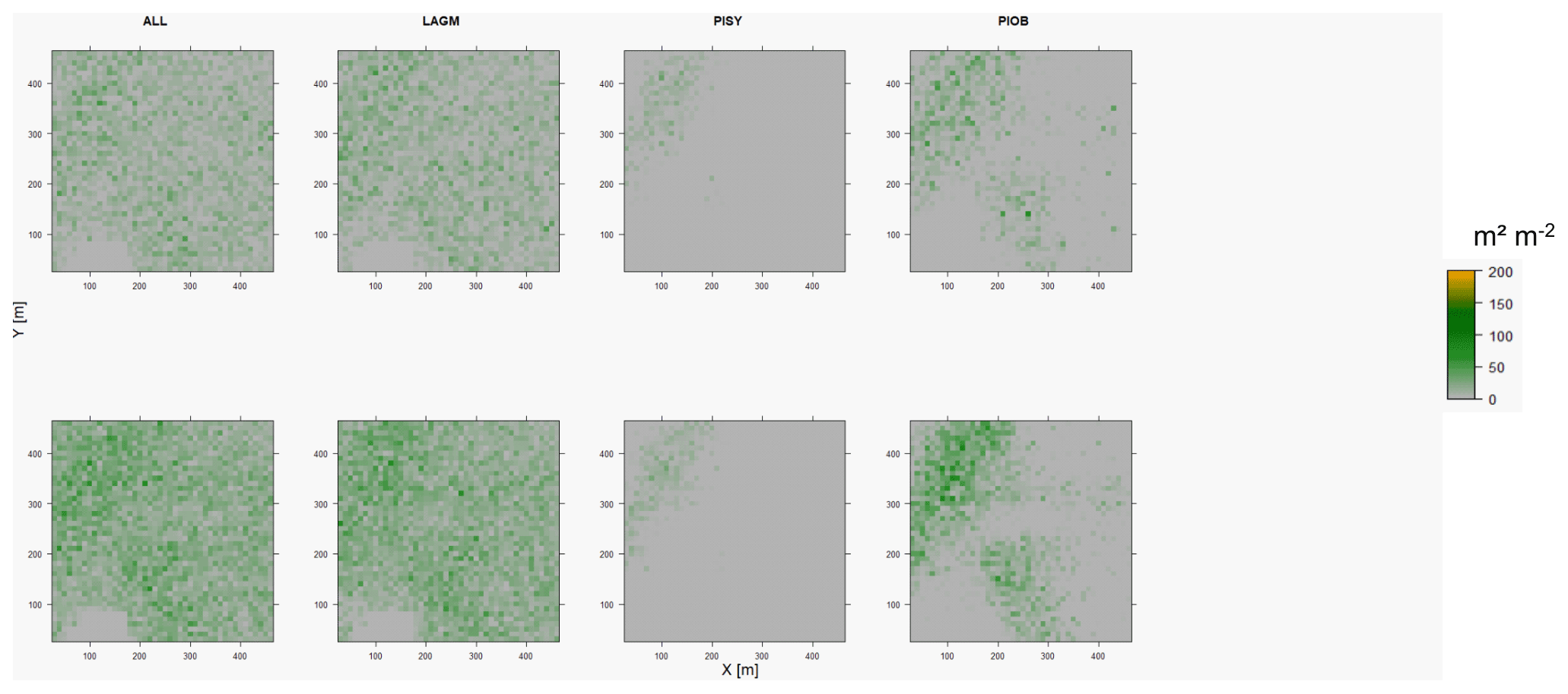
Figure D6Leaf area index (LAI) values of the CryoGrid grid aggregated at year 2020 at Nyurba. Upper row shows LAVESI–CryoGrid coupled; lower row shows LAVESI simulations. LAGM: Larix gmelinii; PIOB: Picea obovata; PISI: Pinus sibirica; PISY: Pinus sylvestris. Simulations with PISI were not possible.
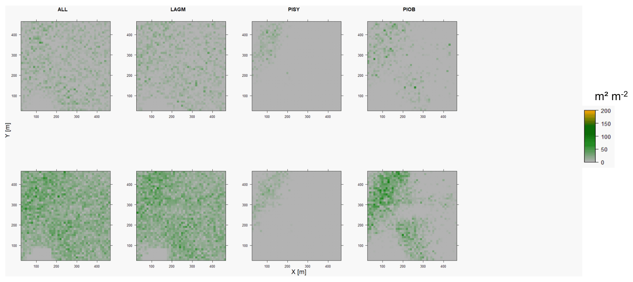
Figure D7Leaf area index (LAI) values of the CryoGrid grid aggregated at year 2025 at Nyurba. Upper row shows LAVESI–CryoGrid coupled; lower row shows LAVESI simulations. LAGM: Larix gmelinii; PIOB: Picea obovata; PISI: Pinus sibirica; PISY: Pinus sylvestris. Simulations with PISI were not possible.
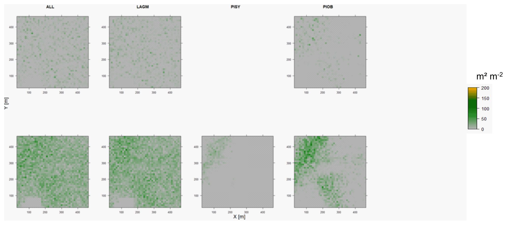
Figure D8Leaf area index (LAI) values of the CryoGrid grid aggregated at year 2030 at Nyurba. Upper row shows LAVESI–CryoGrid coupled; lower row shows LAVESI simulations. LAGM: Larix gmelinii; PIOB: Picea obovata; PISI: Pinus sibirica; PISY: Pinus sylvestris. Simulations with PISI and PISY coupled were not possible.

Figure D9Leaf area index (LAI) values of the CryoGrid grid aggregated at year 2015 at Spasskaya Pad. Upper row shows LAVESI–CryoGrid coupled; lower row shows LAVESI simulations. LAGM: Larix gmelinii; PIOB: Picea obovata; PISI: Pinus sibirica; PISY: Pinus sylvestris.
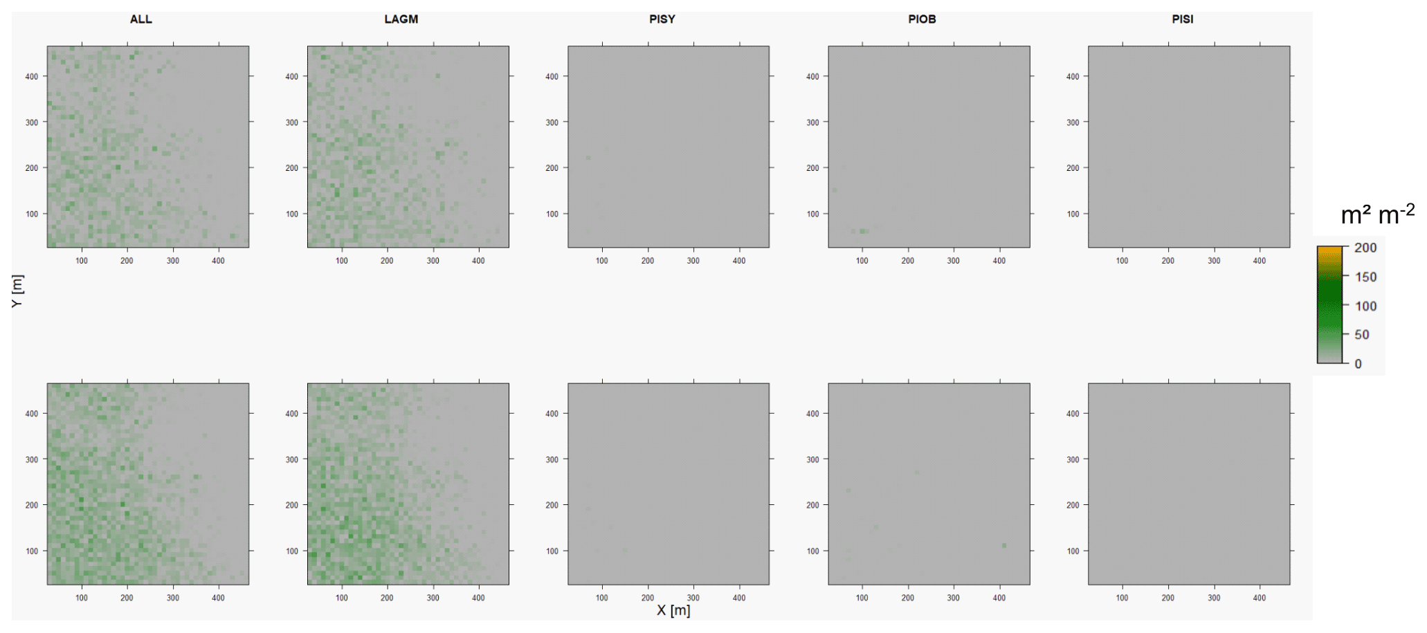
Figure D10Leaf area index (LAI) values of the CryoGrid grid aggregated at year 2020 at Spasskaya Pad. Upper row shows LAVESI–CryoGrid coupled; lower row shows LAVESI simulations. LAGM: Larix gmelinii; PIOB: Picea obovata; PISI: Pinus sibirica; PISY: Pinus sylvestris.
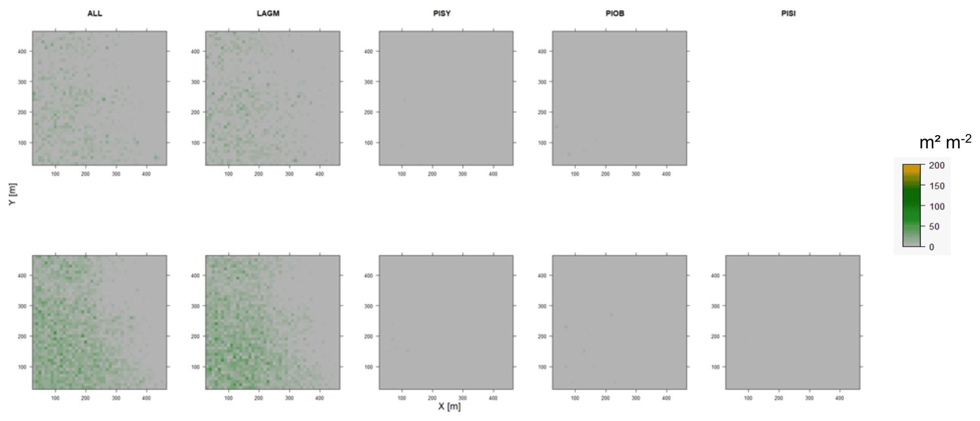
Figure D11Leaf area index (LAI) values of the CryoGrid grid aggregated at year 2025 at Spasskaya Pad. Upper row shows LAVESI–CryoGrid coupled; lower row shows LAVESI simulations. LAGM: Larix gmelinii; PIOB: Picea obovata; PISI: Pinus sibirica; PISY: Pinus sylvestris. Simulations with PISI coupled were not possible.
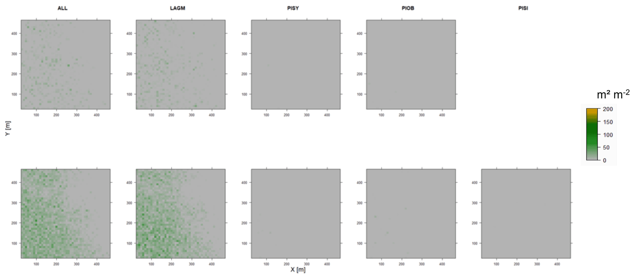
Figure D12Leaf area index (LAI) values of the CryoGrid grid aggregated at year 2030 at Spasskaya Pad. Upper row shows LAVESI–CryoGrid coupled; lower row shows LAVESI simulations. LAGM: Larix gmelinii; PIOB: Picea obovata; PISI: Pinus sibirica; PISY: Pinus sylvestris. Simulations with PISI coupled were not possible.

Figure E1Mean leaf area index aggregated east–west for each simulated focus area and time slice (2010–2030). Upper row shows LAVESI–CryoGrid coupled version; lower row shows only LAVESI.
The CryoGrid code is available on Zenodo (https://doi.org/10.5281/zenodo.5119987, Stuenzi et al., 2021c). The LAVESI branch used for this study is CryoGrid_multispecies, and the commit used for the simulations for this study is 93a9767 tagged as LAVESI–CryoGrid v1.0 (https://github.com/StefanKruse/LAVESI/releases/tag/1.0, last access: 3 February 2022), which is permanently stored on Zenodo (https://doi.org/10.5281/zenodo.5963455, Kruse et al., 2022c). The biomass data and tree-ring growth information for the species present at the region of interest are stored on Zenodo (https://doi.org/10.5281/zenodo.6145386, Kruse et al., 2022b; and https://doi.org/10.5281/zenodo.6145466, Kruse et al., 2022a).
SK and UH initiated the idea of coupling LAVESI with CryoGrid, which was jointly developed by SK, SMS, and ML. SK and SMS set up the coupled version and maintained the simulation runs together. JG developed the upgrade to implement multiple species efficiently in LAVESI, and SK realized the implementation of the LAVESI-related programming. SK analysed the data and drafted the first version of the paper, which was jointly edited by all authors.
The contact author has declared that neither they nor their co-authors have any competing interests.
Publisher's note: Copernicus Publications remains neutral with regard to jurisdictional claims in published maps and institutional affiliations.
We are grateful for the support of Sven N. Willner in parallelizing LAVESI. The data and experience gained on the successful Chukotka and central Yakutia expedition in 2018 was the basis for the developments, and we especially thank Luidmila A. Pestryakova for her support and leadership of the expedition, but we also thank all participants involved in the expedition. We thank Luca Farcas and Christopher Guth for their support in preparing samples and establishing tree-ring chronologies, as well as Ingo Heinrich from the GFZ dendro lab for support with the dendroecological analyses. We thank Iuliia Shevtsova for supporting the organization and analyses of the biomass data. We are especially grateful for the HPC support at AWI, mainly Natalya Rakowski and Malte Thoma for their assistance in the simulation setup. We would like to thank Cathy Jenks as well as two anonymous reviewers for proofreading and their comments that led to an improved version of the paper.
This research has been supported by the European Research Council, H2020 European Research Council (GlacialLegacy (grant no. 772852)), the Bundesministerium für Bildung und Forschung (grant no. 01LN1709A), and the Helmholtz Association (MOSES).
The article processing charges for this open-access publication were covered by the Alfred Wegener Institute, Helmholtz Centre for Polar and Marine Research (AWI).
This paper was edited by Hisashi Sato and reviewed by two anonymous referees.
Abaimov, A. P., Lesinski, J. A., Martinsson, O., and Milyutin, L. I.: Variability and Ecology of Siberian Larch Species, Swedish Univ. of Agricultural Sciences, Umeå (Sweden), Dept. of Silviculture, 75, ISSN 0348-8968, 1998.
Barber, V. A., Juday, G. P., and Finney, B. P.: Reduced growth of Alaskan white spruce in the twentieth century from temperature-induced drought stress, Nature, 405, 668–673, https://doi.org/10.1038/35015049, 2000.
Berner, L. T., Beck, P. S. A., Bunn, A. G., and Goetz, S. J.: Plant response to climate change along the forest-tundra ecotone in northeastern Siberia, Glob. Change Biol., 19, 3449–3462, https://doi.org/10.1111/gcb.12304, 2013.
Biskaborn, B. K., Brieger, F., Herzschuh, U., Kruse, S., Pestryakova, L., Shevtsova, I., Stuenzi, S., Vyse, S., and Zakharov, E.: Glacial lake coring and treeline forest analyses at the northeastern treeline extension in Chukotka, in: Russian-German Cooperation: Expeditions to Siberia in 2018. Berichte zur Polar-und Meeresforschung [Reports on polar and marine research, edited by: Kruse, S., Bolshiyanov, D., Grigoriev, M. N., Morgenstern, A., Pestryakova, L., Tsibizov, L., and Udke, A., Bremerhaven: Alfred Wegener Institute for Polar and Marine Research, 734, 139–147, https://doi.org/10.2312/BzPM_0734_2019, 2019.
Błasiak, A., Węgiel, A., Łukowski, A., Sułkowski, S., and Turski, M.: The effects of tree and stand traits on the specific leaf area in managed scots pine forests of different ages, Forests, 12, 396, https://doi.org/10.3390/f12040396, 2021.
Boike, J., Nitzbon, J., Anders, K., Grigoriev, M., Bolshiyanov, D., Langer, M., Lange, S., Bornemann, N., Morgenstern, A., Schreiber, P., Wille, C., Chadburn, S., Gouttevin, I., Burke, E., and Kutzbach, L.: A 16-year record (2002–2017) of permafrost, active-layer, and meteorological conditions at the Samoylov Island Arctic permafrost research site, Lena River delta, northern Siberia: an opportunity to validate remote-sensing data and land surface, snow, and permafrost models, Earth Syst. Sci. Data, 11, 261–299, https://doi.org/10.5194/essd-11-261-2019, 2019.
Bonan, G. B.: Forests and Climate Change: Forcings, Feedbacks, and the Climate Benefits of Forests, Science, 320, 1444–1449, https://doi.org/10.1126/science.1155121, 2008.
Bonan, G. B., Williams, M., Fisher, R. A., and Oleson, K. W.: Modeling stomatal conductance in the earth system: linking leaf water-use efficiency and water transport along the soil–plant–atmosphere continuum, Geosci. Model Dev., 7, 2193–2222, https://doi.org/10.5194/gmd-7-2193-2014, 2014.
Bunn, A., Korpela, M., Biondi, F. Campelo, F., Mérian, P., Qeadan, F., and Zang, C.: dplR: Dendrochronology Program Library in R. R package version 1.7.1, https://CRAN.R-project.org/package=dplR (last access: 3 January 2018), 2020.
Chen, H. Y., Klinka, K., Mathey, A.-H., Wang, X., Varga, P., and Chourmouzis, C.: Are mixed-species stands more productive than single-species stands: an empirical test of three forest types in British Columbia and Alberta, Can. J. Forest Res., 33, 1227–1237, https://doi.org/10.1139/x03-048, 2003.
Churakova, O. V., Siegwolf, R. T. W., Fonti, M. V., Vaganov, E. A., and Saurer, M.: Spring arctic oscillation as a trigger of summer drought in Siberian subarctic over the past 1494 years, Sci. Rep.-UK, 11, 1–10, https://doi.org/10.1038/s41598-021-97911-2, 2021.
Conrad, O., Bechtel, B., Bock, M., Dietrich, H., Fischer, E., Gerlitz, L., Wehberg, J., Wichmann, V., and Böhner, J.: System for Automated Geoscientific Analyses (SAGA) v. 2.1.4, Geosci. Model Dev., 8, 1991–2007, https://doi.org/10.5194/gmd-8-1991-2015, 2015.
DeAngelis, D. L. and Mooij, W. M.: Individual-based modeling of ecological and evolutionary processes, Annu. Rev. Ecol. Evol. Syst., 36, 147–168, https://doi.org/10.1146/annurev.ecolsys.36.102003.152644, 2005.
ESA: Land Cover CCI Product User Guide Version 2. Tech. Rep., http://maps.elie.ucl.ac.be/CCI/viewer/download/ESACCI-LC-Ph2-PUGv2_2.0.pdf (last access: 17 February 2022), 2017.
Gorelick, N., Hancher, M., Dixon, M., Ilyushchenko, S., Thau, D., and Moore, R.: Google Earth Engine: Planetary-scale geospatial analysis for everyone, Remote Sens. Environ., 202, 18–27, https://doi.org/10.1016/j.rse.2017.06.031, 2017.
Grimm, V. and Railsback, S. F.: Individual-based Modeling and Ecology, Princeton University Press, Princeton, NJ, ISBN 978-0-691-09666-7, 2005.
Grimm, V., Berger, U., DeAngelis, D. L., Polhill, J. G., Giske, J., and Railsback, S. F.: The ODD protocol: A review and first update, Ecol. Model., 221, 2760–2768, https://doi.org/10.1016/j.ecolmodel.2010.08.019, 2010.
Harris, I., Osborn, T. J., Jones, P., and Lister, D.: Version 4 of the CRU TS monthly high-resolution gridded multivariate climate dataset, Sci Data, 7, 1–18, https://doi.org/10.1038/s41597-020-0453-3, 2020.
Hersbach, H., Bell, B., Berrisford, P., Hirahara, S., Horányi, A., Muñoz-Sabater, J., Nicolas, J., Peubey, C., Radu, R., Schepers, D., Simmons, A., Soci, C., Abdalla, S., Abellan, X., Balsamo, G., Bechtold, P., Biavati, G., Bidlot, J., Bonavita, M., De Chiara, G., Dahlgren, P., Dee, D., Diamantakis, M., Dragani, R., Flemming, J., Forbes, R., Fuentes, M., Geer, A., Haimberger, L., Healy, S., Hogan, R. J., Hólm, E., Janisková, M., Keeley, S., Laloyaux, P., Lopez, P., Lupu, C., Radnoti, G., de Rosnay, P., Rozum, I., Vamborg, F., Villaume, S., and Thépaut, J.-N.: The ERA5 global reanalysis, Q. J. Roy. Meteor. Soc., 146, 1999–2049, https://doi.org/10.1002/qj.3803, 2020.
Herzschuh, U.: Legacy of the Last Glacial on the present-day distribution of deciduous versus evergreen boreal forests, Global Ecol. Biogeogr., 29, 198–206, https://doi.org/10.1111/geb.13018, 2020.
Herzschuh, U., Birks, H. J. B., Laepple, T., Andreev, A., Melles, M., and Brigham-Grette, J.: Glacial legacies on interglacial vegetation at the Pliocene-Pleistocene transition in NE Asia, Nat. Commun., 7, 1–11, https://doi.org/10.1038/ncomms11967, 2016.
Hijmans, R. J.: raster: Geographic Data Analysis and Modeling. R package version 3.0-12, https://CRAN.R-project.org/package=raster (last access: 30 March 2021), 2020.
Kharuk, V., Ranson, K., and Dvinskaya, M.: Evidence of Evergreen Conifer Invasion into Larch Dominated Forests During Recent Decades in Central Siberia, Eurasian J. For. Res., 10, 163–171, 2007.
Kharuk, V. I., Im, S. T., Petrov, I. A., Dvinskaya, M. L., Shushpanov, A. S., and Golyukov, A. S.: Climate-driven conifer mortality in Siberia, Global Ecol. Biogeogr., 30, 543–556, https://doi.org/10.1111/geb.13243, 2021.
Kirpotin, S. N., Callaghan, T. V., Peregon, A. M., Babenko, A. S., Berman, D. I., Bulakhova, N. A., Byzaakay, Arysia A. Chernykh, T. M., Chursin, V., Interesova, E. A., Gureev, S. P., Kerchev, I. A., Kharuk, V. I., Khovalyg, A. O., Kolpashchikov, L. A., Krivets, S. A., Kvasnikova, Z. N., Kuzhevskaia, I. V., Merzlyakov, O. E., Nekhoroshev, O. G., Popkov, V. K., Pyak, A. I., Valevich, T. O., Volkov, I. V., and Volkova, I. I.: Impacts of environmental change on biodiversity and vegetation dynamics in Siberia, Ambio, 50, 1926–1952, https://doi.org/10.1007/s13280-021-01570-6, 2021.
Konôpková, A., Vedernikov, K. E., Zagrebin, E. A., Islamova, N. A., Grigoriev, R. A., Húdoková, H., Petek, A, Kmeť, J., Petrík, P., Pashkova, A. S., Zhuravleva, A. N., and Bukharina, I. L.: Impact of the European bark beetle Ips typographus on biochemical and growth properties of wood and needles in Siberian spruce Picea obovata, Central European Forestry Journal, 66, 243–254, https://doi.org/10.2478/forj-2020-0025, 2020.
Krieger, G., Moreira, A., Fiedler, H., Hajnsek, I., Werner, M., Younis, M., and Zink, M.: TanDEM-X: A satellite formation for high-resolution SAR interferometry, IEEE T. Geosci. Remote, 45, 3317–3340, https://doi.org/10.1109/TGRS.2007.900693, 2007.
Kruse, S., Wieczorek, M., Jeltsch, F., and Herzschuh, U.: Treeline dynamics in Siberia under changing climates as inferred from an individual-based model for Larix, Ecol. Model., 338, 101–121, https://doi.org/10.1016/j.ecolmodel.2016.08.003, 2016.
Kruse, S., Gerdes, A., Kath, N. J., and Herzschuh, U.: Implementing spatially explicit wind-driven seed and pollen dispersal in the individual-based larch simulation model: LAVESI-WIND 1.0, Geosci. Model Dev., 11, 4451–4467, https://doi.org/10.5194/gmd-11-4451-2018, 2018.
Kruse, S., Gerdes, A., Kath, N. J., Epp, L. S., Stoof-Leichsenring, K. R., Pestryakova, L. A., and Herzschuh, U.: Dispersal distances and migration rates at the arctic treeline in Siberia – a genetic and simulation-based study, Biogeosciences, 16, 1211–1224, https://doi.org/10.5194/bg-16-1211-2019, 2019a.
Kruse, S., Herzschuh, U., Stünzi, S., Vyse, S., and Zakharov, E.: Sampling mixed-species boreal forests affected by disturbances and mountain lake and alas lake coring in Central Yakutia, in: Kruse, S., Bolshiyanov, D., Grigoriev, M. N., Morgenstern, A., Pestryakova, L., Tsibizov, L., and Udke, A., Russian-German Cooperation: Expeditions to Siberia in 2018, Berichte zur Polar-und Meeresforschung [Reports on polar and marine research], Alfred Wegener Institute for Polar and Marine Research, Bremerhaven, 148–153, https://doi.org/10.2312/BzPM_0734_2019, 2019b.
Kruse, S., Kolmogorov, A. I., Pestryakova, L. A., and Herzschuh, U.: Long-lived larch clones may conserve adaptations that could restrict treeline migration in northern Siberia, Ecol. Evol., 10, 10017–10030, https://doi.org/10.1002/ece3.6660, 2020.
Kruse, S., Frommel, I., Nitsche, C., Balanzategui, D., Heinrich, I., Herzschuh, U., Brieger, F., Schulte, L., Stuenzi, S. M., Pestryakova, L. A., and Zakharov, E. S.: Tree ring width chronologies of four Pinaceae species in boreal forests in Yakutia in 2018 (1.0), Zenodo [data set], https://doi.org/10.5281/zenodo.6145466, 2022a.
Kruse, S., Herzschuh, U., Shevtsova, I., Brieger, F., Schulte, L., Stuenzi, S. M., Pestryakova, L. A., and Zakharov, E. S.: Individual tree aboveground biomass of four Pinaceae species in boreal forests in Yakutia in 2018 (1.0), Zenodo [data set], https://doi.org/10.5281/zenodo.6145386, 2022b.
Kruse, S., Stuenzi, S. M., and Gloy, J.: StefanKruse/LAVESI: LAVESI-CryoGrid v1.0 (1.0), Zenodo [code], https://doi.org/10.5281/zenodo.5963455, 2022c.
Kuznetsova, L. V., Zakharova, V. I., Sosina, N. K., Nikolin, E. G., Ivanova, E. I., Sofronova, E. V., Poryadina, L, N., Mikhalyova, L. G., Vasilyeva, I. I., Remigailo, P. A., Gabyshev, V. A., Ivanova, A. P., and Kopyrina, L. I.: Flora of Yakutia: Composition and Ecological Structure, in: The Far North: Plant Biodiversity and Ecology of Yakutia, edited by: Troeva, E. I., Isaev, A. P., Cherosov, M. M., and Karpov, N. S., Springer, Dordrecht, the Netherlands, 3, 357–369, https://doi.org/10.1007/978-90-481-3774-9, 2010.
Langer, M., Westermann, S., Muster, S., Piel, K., and Boike, J.: The surface energy balance of a polygonal tundra site in northern Siberia – Part 1: Spring to fall, The Cryosphere, 5, 151–171, https://doi.org/10.5194/tc-5-151-2011, 2011.
Lawrence, D. M., Koven, C. D., Swenson, S. C., Riley, W. J., and Slater, A. G.: Permafrost thaw and resulting soil moisture changes regulate projected high-latitude CO2 and CH4 emissions, Environ. Res. Lett., 10, 94011, https://doi.org/10.1088/1748-9326/10/9/094011, 2015.
Lehsten, V., Mischurow, M., Lindström, E., Lehsten, D., and Lischke, H.: LPJ-GM 1.0: simulating migration efficiently in a dynamic vegetation model, Geosci. Model Dev., 12, 893–908, https://doi.org/10.5194/gmd-12-893-2019, 2019.
Liang, J., Crowther, T. W., Picard, N., Wiser, S., Zhou, M., Alberti, G., Schulze, E.-D., McGuire, A. D., Bozzato, F.,Pretzsch, H., de-Miguel, S., Paquette, A., Hérault, B., Scherer-Lorenzen, M., Barrett, C. B., Glick, H. B., Hengeveld, G. M., Nabuurs, G.-J., Pfautsch, S., Viana, H., Vibrans, A. C., Ammer, C., Schall, P., Verbyla, D., Tchebakova, N., Fischer, M., Watson, J. V., Chen, H. Y. H., Lei, X., Schelhaas, M.-J., Lu, H., Gianelle, D., Parfenova, E. I., Salas, C., Lee, E., Lee, B., Kim, H. S., Bruelheide, H., Coomes, D. A., Piotto, D., Sunderland, T., Schmid, B.,Gourlet-Fleury, S., Sonké, B., Tavani, R., Zhu, J., Brandl, S., Vayreda, J., Kitahara, F., Searle, E. B., Neldner, V. J., Ngugi, M. R., Baraloto, C., Frizzera, L., Bałazy, R., Oleksyn, J., Zawiła-Niedźwiecki, T., Bouriaud, O., Bussotti, F., Finér, L., Jaroszewicz, B., Jucker, T., Valladares, F., Jagodzinski, A. M., Peri, P. L., Gonmadje, C., Marthy, W., O'Brien, T., Martin, E. H., Marshall, A. R., Rovero, F., Bitariho, R., Niklaus, P. A., Alvarez-Loayza, P., Chamuya, N., Valencia, R., Mortier, F., Wortel, V., Engone-Obiang, N. L., Ferreira, L. V., Odeke, D. E., Vasquez, R. M., Lewis, S. L., and Reich, P. B.: Positive biodiversity-productivity relationship predominant in global forests, Science, 354, 6309, https://doi.org/10.1126/science.aaf8957, 2016.
Liang, M., Sugimoto, A., Tei, S., Bragin, I. V., Takano, S., Morozumi, T., Shingubara, R., Maximov, T. C., Kiyashko, S. I. Velivetskaya, T. A., and Ignatiev, A. V.: Importance of soil moisture and N availability to larch growth and distribution in the Arctic taiga-tundra boundary ecosystem, northeastern Siberia, Polar Sci., 8, 327–341, https://doi.org/10.1016/j.polar.2014.07.008, 2014.
MacDonald, G. M., Kremenetski, K. V., and Beilman, D. W.: Climate change and the northern Russian treeline zone, Philos. T. Roy. Soc. B, 363, 2283–2299, https://doi.org/10.1098/rstb.2007.2200, 2008.
Mamet, S. D., Brown, C. D., Trant, A. J., and Laroque, C. P.: Shifting global Larix distributions: Northern expansion and southern retraction as species respond to changing climate, J. Biogeogr., 46, 30–44, https://doi.org/10.1111/jbi.13465, 2019.
Mencuccini, M. and Bonosi, L.: Leaf/sapwood area ratios in Scots pine show acclimation across Europe, Can. J. Forest Res., 31, 442–456, https://doi.org/10.1139/cjfr-31-3-442, 2001.
Nitzbon, J., Langer, M., Westermann, S., Martin, L., Aas, K. S., and Boike, J.: Pathways of ice-wedge degradation in polygonal tundra under different hydrological conditions, The Cryosphere, 13, 1089–1123, https://doi.org/10.5194/tc-13-1089-2019, 2019.
Ohta, T., Vol, H. P., Hiyama, T., Tanaka, H., Kuwada, T., Maximov, T. C., Ohata, T., Fukushima, Y., Sciences, H., Problems, B., Science, L. T., Change, G., and Faculty, T. O.: Seasonal Variation in the Energy and Water Exchanges above and below a Larch Forest in Eastern Siberia, Hydrol. Process., 15, 1459–1476, https://doi.org/10.1002/hyp.219, 2001.
Pinheiro, J., Bates, D., DebRoy, S., and Sarkar, D.: nlme: Linear and Nonlinear Mixed Effects Models, R package version 3.1-140, https://CRAN.R-project.org/package=nlme (last access: 30 June 2019), 2019.
R Core Team: R: A Language and Environment for Statistical Computing, Vienna, Austria, https://www.r-project.org/ (last access: 10 January 2020), 2019.
Rees, W. G., Hofgaard, A., Boudreau, S., Cairns, D. M., Harper, K., Mamet, S., Mathisen, I., Swirad, Z., and Tutubalina, O.: Is subarctic forest advance able to keep pace with climate change?, Glob. Change Biol., 26, 3965–3977, https://doi.org/10.1111/gcb.15113, 2020.
Reich, P. B., Walters, M. B., Ellsworth, D. S., Vose, J. M., Voliin, J. C., Gresham, C., and Bowman, W. D.: Relationships of leaf dark respiration to leaf nitrogen, specific leaf area and leaf life-span: a test across biomes and functional groups, Oecologia, 114, 471–482, https://doi.org/10.1007/s004420050471, 1998.
Sarkar, D.: Lattice: Multivariate Data Visualization with R, Springer, New York, ISBN 978-0-387-75968-5, 2008.
Sato, H., Kobayashi, H., Iwahana, G., and Ohta, T.: Endurance of larch forest ecosystems in eastern Siberia under warming trends, Ecol. Evol., 6, 5690–5704, https://doi.org/10.1002/ece3.2285, 2016.
Shevtsova, I., Kruse, S., Herzschuh, U., Brieger, F., Schulte, L., Stuenzi, S. M., Pestryakova, L. A., and Zakharov, E. S.: Individual tree and tall shrub partial above-ground biomass of central Chukotka in 2018, PANGAEA [data set], https://doi.org/10.1594/PANGAEA.923784, 2020.
Shevtsova, I., Herzschuh, U., Heim, B., Schulte, L., Stünzi, S., Pestryakova, L. A., Zakharov, E. S., and Kruse, S.: Recent above-ground biomass changes in central Chukotka (Russian Far East) using field sampling and Landsat satellite data, Biogeosciences, 18, 3343–3366, https://doi.org/10.5194/bg-18-3343-2021, 2021.
Snell, R. S.: Simulating long-distance seed dispersal in a dynamic vegetation model, Global Ecol. Biogeogr., 23, 89–98, https://doi.org/10.1111/geb.12106, 2014.
Snell, R. S. and Cowling, S. A.: Consideration of dispersal processes and northern refugia can improve our understanding of past plant migration rates in North America, J. Biogeogr., 42, 1677–1688, https://doi.org/10.1111/jbi.12544, 2015.
Stocker, B. D., Roth, R., Joos, F., Spahni, R., Steinacher, M., Zaehle, S., Bouwman, L., and Prentice, I. C.: Multiple greenhouse-gas feedbacks from the land biosphere under future climate change scenarios, Nat. Clim. Change, 3, 666–672, https://doi.org/10.1038/nclimate1864, 2013.
Stuenzi, S. M., Boike, J., Cable, W., Herzschuh, U., Kruse, S., Pestryakova, L. A., Schneider von Deimling, T., Westermann, S., Zakharov, E. S., and Langer, M.: Variability of the surface energy balance in permafrost-underlain boreal forest, Biogeosciences, 18, 343–365, https://doi.org/10.5194/bg-18-343-2021, 2021a.
Stuenzi, S. M., Boike, J., Gädecke, A., Herzschuh, U., Kruse, S., Pestryakova, L. A., Westermann, S., and Langer, M.: Variability of the surface energy balance in permafrost-underlain boreal forest, ERL, 16, 084045, https://doi.org/10.1088/1748-9326/ac153d, 2021b.
Stuenzi, S. M., Kruse, S., Boike, J., Herzschuh, U., Westermann, S., and Langer, M.: Coupled multilayer canopy-permafrost model (CryoGrid) for the use with an individual-based larch vegetation simulator (LAVESI), Zenodo [code], https://doi.org/10.5281/zenodo.5119987, 2021c.
Sugimoto, A., Yanagisawa, N., Naito, D., Fujita, N., and Maximov, T. C.: Importance of permafrost as a source of water for plants in east Siberian taiga, Ecol. Res., 17, 493–503, https://doi.org/10.1046/j.1440-1703.2002.00506.x, 2002.
Walker, D. A., Raynolds, M. K., Daniëls, F. J. A. A., Einarsson, E., Elvebakk, A., Gould, W. A., Katenin, A. E., Kholod, S. S., Markon, C. J., Melnikov, E. S., Moskalenko, N. G., Talbot, S. S., Yurtsev, B. A., and the other members of the CAVM Team: The circumpolar Arctic vegetation map, J. Veg. Sci., 16, 267–282, https://doi.org/10.1658/1100-9233(2005)016[0267:TCAVM]2.0.CO;2, 2005.
Westermann, S., Langer, M., Boike, J., Heikenfeld, M., Peter, M., Etzelmüller, B., and Krinner, G.: Simulating the thermal regime and thaw processes of ice-rich permafrost ground with the land-surface model CryoGrid 3, Geosci. Model Dev., 9, 523–546, https://doi.org/10.5194/gmd-9-523-2016, 2016.
Wieczorek, M., Kruse, S., Epp, L. S., Kolmogorov, A., Nikolaev, A. N., Heinrich, I., Jeltsch, F., Pestryakova, L. A., Zibulski, R., and Herzschuh, U.: Dissimilar responses of larch stands in northern Siberia to increasing temperatures-a field and simulation based study, Ecology, 98, 2343–2355, https://doi.org/10.1002/ecy.1887, 2017.
Xian-Kui, Q. and Chuan-Kuan, W.: Comparison of foliar water use efficiency among 17 provenances of Larix gmelinii in the Mao'ershan area, Chinese Journal of Plant Ecology, 39, 352–361, https://doi.org/10.17521/cjpe.2015.0034, 2015.
Yoo, A. B., Jette, M. A., and Grondona, M.: SLURM: Simple Linux Utility for Resource Management. Lect Notes Comput Sc (including subseries Lecture Notes in Artificial Intelligence and Lecture Notes in Bioinformatics), 2862, 44–60, https://doi.org/10.1007/10968987_3, 2003.
Zeller, L., Liang, J., and Pretzsch, H.: Tree species richness enhances stand productivity while stand structure can have opposite effects, based on forest inventory data from Germany and the United States of America, Forest Ecosyst., 5, 4, https://doi.org/10.1186/s40663-017-0127-6, 2018.
Zhang, W., Miller, P. A., Smith, B., Wania, R., Koenigk, T., and Döscher, R.: Tundra shrubification and tree-line advance amplify Arctic climate warming: results from an individual-based dynamic vegetation model, Environ. Res. Lett., 8, 034023, https://doi.org/10.1088/1748-9326/8/3/034023, 2013.
Zweigel, R. B., Westermann, S., Nitzbon, J., Langer, M., Boike, J., Etzelmüller, B., and Schuler, T. V.: Simulating snow redistribution and its effect on ground surface temperature at a high-Arctic site on Svalbard, J. Geophys. Res.-Earth Surf., 126, e2020JF005673, https://doi.org/10.1029/2020jf005673, 2021.
- Abstract
- Introduction
- Methods
- Results
- Discussion
- Conclusions
- Appendix A
- Appendix B: Landscape defining the focus region's plot area
- Appendix C: CryoGrid model parameters and constants used
- Appendix D: Spatial distribution of the leaf area index (LAI) for mixed-species and pure-species simulations at the focus regions in 5-year steps
- Appendix E: Evolution of leaf area index (LAI) across the focus region simulation areas
- Data availability
- Author contributions
- Competing interests
- Disclaimer
- Acknowledgements
- Financial support
- Review statement
- References