the Creative Commons Attribution 4.0 License.
the Creative Commons Attribution 4.0 License.
 | 17 Mar 2022
Earth system model parameter adjustment using a Green's functions approach
Andrea Molod
Donifan Barahona
Atanas Trayanov
Dimitris Menemenlis
Gael Forget
We demonstrate the practicality and effectiveness of using a Green's functions estimation approach for adjusting uncertain parameters in an Earth system model (ESM). This estimation approach has previously been applied to an intermediate-complexity climate model and to individual ESM components, e.g., ocean, sea ice, or carbon cycle components. Here, the Green's functions approach is applied to a state-of-the-art ESM that comprises a global atmosphere/land configuration of the Goddard Earth Observing System (GEOS) coupled to an ocean and sea ice configuration of the Massachusetts Institute of Technology general circulation model (MITgcm). Horizontal grid spacing is approximately 110 km for GEOS and 37–110 km for MITgcm. In addition to the reference GEOS-MITgcm simulation, we carried out a series of model sensitivity experiments, in which 20 uncertain parameters are perturbed. These “control” parameters can be used to adjust sea ice, microphysics, turbulence, radiation, and surface schemes in the coupled simulation. We defined eight observational targets: sea ice fraction, net surface shortwave radiation, downward longwave radiation, near-surface temperature, sea surface temperature, sea surface salinity, and ocean temperature and salinity at 300 m. We applied the Green's functions approach to optimize the values of the 20 control parameters so as to minimize a weighted least-squares distance between the model and the eight observational targets. The new experiment with the optimized parameters resulted in a total cost reduction of 9 % relative to a simulation that had already been adjusted using other methods. The optimized experiment attained a balanced cost reduction over most of the observational targets. We also report on results from a set of sensitivity experiments that are not used in the final optimized simulation but helped explore options and guided the optimization process. These experiments include an assessment of sensitivity to the number of control parameters and to the selection of observational targets and weights in the cost function. Based on these sensitivity experiments, we selected a specific definition for the cost function. The sensitivity experiments also revealed a decreasing overall cost as the number of control variables was increased. In summary, we recommend using the Green's functions estimation approach as an additional fine-tuning step in the model development process. The method is not a replacement for modelers' experience in choosing and adjusting sensitive model parameters. Instead, it is an additional practical and effective tool for carrying out final adjustments of uncertain ESM parameters.
- Article
(3197 KB) - Full-text XML
- BibTeX
- EndNote


Earth system models (ESMs) include various parameters that govern the representation of unresolved, unrepresented, or underobserved processes in the models. The most sensitive parameters are typically adjusted during the last step of model development relative to observational targets. Currently, there is no agreed-upon methodology to adjust model parameters. As an illustration of the range of approaches and observational targets, Schmidt et al. (2017) describe the vast range of tuning strategies used for ESM development in US modeling centers. Parameter adjustment aims to improve the representation of various processes or key state fields in the model relative to a predetermined set of observational targets (Mauritsen et al., 2012; Hourdin et al., 2017).
ESM tuning is often done in a heuristic, trial-and-error manner, wherein one or more parameters are perturbed to new values based on diagnosing the causes of systematic error with the aim of improving the model's overall behavior (e.g., Watanabe et al., 2010; Yukimoto et al., 2012; Mauritsen et al., 2019; Voldoire et al., 2019; Golaz et al., 2019; Sellar et al., 2019; Danabasoglu et al., 2020). The observational targets can include, for example, radiation balance at the top of the atmosphere, surface temperature, sea ice variability, tropospheric wind, or even a derived target such as a “cloud object” (Posselt et al., 2015). In this approach, a typical tuning exercise comprises several iterations of suites of sensitivity experiments with one or more perturbed parameters. After each iteration, a comparison is performed against a set of observations, and another set of sensitivity experiments targeting either the same or another set of parameters and observations is conducted based on the results. This tuning exercise is highly dependent on the experience and expertise of model developers and on the application for which the model will be used.
There are three main drawbacks of heuristic optimization approaches. The first is that this method necessitates an analysis step between each sensitivity sweep, a time-consuming process. The second drawback is the large number of required simulations, since a new set of experiments is required for iteration of the process. The third drawback is the interdependence of each parameter's effect on the resulting ESM simulation. For example, both sea ice albedo and precipitation efficiency could affect the globally averaged radiation balance at the top of the atmosphere. The adjustment of one parameter or set of parameters at a time is suboptimal, because estimates of empirical parameters depend on each other and on model configuration, boundary conditions, etc.
Given unrestricted computer resources, one could randomly explore model parameter space exhaustively and choose the simulation that best fits all available observations. In practice, this type of exhaustive parameter exploration is not feasible, and we need tractable methods that combine objective methodologies with the model developer's experience to arrive at an optimized choice of model parameters.
To mitigate the drawbacks and computational cost of the above approaches, a number of more objective parameter calibration methods have been proposed for systematically choosing or fine-tuning the final set of optimized parameters. These methods include the use of Latin hypercube sampling techniques (Posselt et al., 2015), the downhill simplex method (Zhang et al., 2015), the multiple very fast simulated annealing (Zou et al., 2014), and Gauss–Newton line search algorithms (Tett et al., 2013, 2017; Roach et al., 2018). The above estimation methods require a large suite of experiments, which are computationally expensive. Therefore, the sensitivity experiments are typically carried out with very low resolution, atmosphere-only, or even single-column model configurations. The direct applicability of these methods for tuning an ESM may consequently be limited.
Another alternative to heuristic estimation approaches is the adjoint method. Using the adjoint method, one can adjust many parameters simultaneously. A successful example is provided by the Estimating the Circulation and Climate of the Ocean (ECCO) consortium, which used the adjoint method to adjust Massachusetts Institute of Technology general circulation model (MITgcm) ocean model parameters, initial conditions, and boundary conditions (Forget et al., 2015). Although the adjoint method provides robust results, developing a model's adjoint is time consuming, even when using an automatic differentiation software tool. Additionally, the adjoint method is computationally expensive because many forward-adjoint ESM simulations would be required to optimize a nonlinear model.
In this study, we will explore the applicability of the Green's functions approach of Menemenlis et al. (2005) to the calibration of an ESM – the Goddard Earth Observing System (GEOS) land/atmosphere model coupled to the MITgcm ocean model. Compared to other methods, the key advantages of the Green’s function approach are simplicity of implementation, robustness in the presence of nonlinearities, and explicit computation of the data kernel matrix. Compared to heuristic, trial-and-error approaches, the Green's functions approach optimizes uncertain parameters all at once as opposed to one at a time, hence taking into account linear dependencies between these parameters. Therefore, the Green's functions approach accounts for the combined impact of all the parameters while also establishing the individual impact of any one parameter on the solution and with respect to each observational target. Once the forward-model sensitivity experiments have been carried out, the optimization step can be repeated using different observational targets and weights at very small additional computational cost. Assuming that the linearization assumptions hold, only one forward-model sensitivity experiment is required per parameter to be adjusted, which reduces the computational cost relative to the heuristic and objective approaches listed in the previous paragraphs. While the application of an adjoint model requires substantial additional model development and coding efforts, all that is required to apply the Green’s function approach is the computation of ESM forward sensitivity experiments. Furthermore, while the adjoint method would require that the exact tangent linear of the ESM be well behaved, Green's functions provide an approximate linearization, which can be used to reduce the cost function even when the adjoint model is ill behaved. Finally, the explicit computation of the data kernel matrix makes available a vast array of tools from discrete linear inverse theory for deriving and analyzing the solutions.
The key drawback of the Green’s function approach is that computational cost increases linearly with the number of control parameters. Therefore, the method is only applicable to situations where a small number of control parameters need to be estimated. Despite these drawbacks, we will demonstrate that the Green's functions approach can be an invaluable addition to the repertoire of estimation tools used to adjust ESM model parameters.
The remainder of the paper is organized as follows: the mathematical formalism and the Green's functions method are presented in the next section. This presentation is followed by a description of the model, the experiments, and the used observational targets. Section 4 presents our chosen configuration results, followed by a section outlining the motivation for the configuration choices. Summary and conclusions are in Sect. 6.
The model used for this study is the GEOS-MITgcm coupled model. We briefly describe here the particular configurations of these two models as they are used in our study. The dynamical core and suite of physical parameterizations of the GEOS Atmospheric General Circulation Model (AGCM), along with the land model and aerosol model, are described in Molod et al. (2020) and in references therein. The turbulent surface layer parameterization, relevant for this study, is a modified version of the parameterization documented in Helfand and Schubert (1995). The wind stress and surface roughness model was modified by the updates of Garfinkel et al. (2011) for a mid-range of wind speeds and further modified by the updates of Molod et al. (2013) for high winds. The GEOS AGCM's cubed-sphere grid was configured to run with a nominal horizontal grid spacing of 100 km. The vertical grid is a hybrid sigma-pressure grid with 72 levels. The time step of integration was set to 450 s.
MITgcm has a finite-volume dynamical core (Marshall et al., 1997). It has a nonlinear free-surface and real freshwater flux (Adcroft and Campin, 2004) and a nonlocal K-profile parameterization scheme for mixing (Large et al., 1994). The MITgcm horizontal grid is the so-called Lat-Lon-Cap (Forget et al., 2015), and was configured to run with a nominal grid spacing of 100 km. The vertical grid is the z* height coordinates (Adcroft and Campin, 2004) and has 50 vertical levels. The time step of integration was set to 450 s, similar to the atmospheric model.
The GEOS-MITgcm atmosphere–ocean interface includes a skin layer (Price et al., 1978), configured for the simulations described here to impose a 1 d timescale on the interaction, and the communication between the ocean and atmosphere is updated at every atmospheric model time step (450 s). The sea ice dynamics model is provided by MITgcm and the sea ice thermodynamics model is from CICE 4.1 (Hunke and Lipscomb, 2010).
Algebraically, the ESM described in Sect. 2 can be expressed as a set of rules for time stepping a state vector,
where x(ti) is a discretized representation of the Earth system at time ti and function Mi represents ESM time-stepping rules for advancing the state vector from time ti to ti+1. The discretized evolution of the true Earth system, xt(ti), is assumed to differ from that of the numerical model by a vector of stochastic perturbations, η, so that
where η is assumed to have zero mean and covariance matrix Q. Consider a set of observations represented by vector yo, which are related to the discretized, time-evolving Earth system state vector by measurement function H, that is,
where ε represents a vector noise process assumed to have zero mean and covariance matrix R. In addition to measurement errors, vector ε includes all model and estimation “representation” errors, i.e., model data residuals that cannot be represented by Mi and η.
To fit the ESM to the available observations, we aim to minimize an objective cost function
which penalizes a weighted least-squares distance between optimized and prior model parameters (ηTQ−1η) and a weighted least-squares distance between simulation and observations (εTR−1ε), where T is the transpose operator and −1 indicates matrix inversion. It can be shown that minimization of Eq. (4) will produce the maximum likelihood solution for Gaussian inverse problems (Kalnay, 2002). For the Green's functions approach, we adjust a small, carefully chosen set of parameters η. To do this, we combine Eqs. (2) and (3) to obtain
where G represents a function of the combination of observation operator H with ESM time-stepping rules Mi. We assume that Eq. (5) can be linearized about a reference ESM simulation so that
where 0 is a null vector, G(0) represents the reference ESM simulation sampled by measurement function H, vector yd is the model data difference between observations and the reference simulation, and kernel matrix G can be thought of as a first-order multivariate Taylor expansion of G around η=0. The assumption here is that for a small enough perturbation, the model response is linear. Kernel matrix G can be derived by conducting an ESM perturbation experiment for each element of vector η. Specifically, the jth column of matrix G is
where ej is a perturbation vector filled with zeros except for element j, which is perturbed by scalar value ej. The minimization of Eq. (4) given Eq. (5) is a discrete linear inverse problem with solution
where
is the uncertainty covariance matrix for the optimized estimate ηa. Mathematically, the Green's function approach is equivalent to any linear Gaussian inverse problem, e.g., the adjoint method.
In practice, the Green's functions estimation method can be divided into the following six steps:
-
Run a reference ESM simulation using default values for model error parameters, i.e., η=0. The output from this experiment, sampled by observation operator H, provides G(0) in Eqs. (5) and (6).
-
Choose a set of observational targets, i.e., define operator H and vector yo in Eq. (3).
-
Estimate error covariance matrices Q and R – the model and observation/representation errors, respectively – that are needed to define cost function J in Eq. (4).
-
Run a set of model sensitivity experiments, where each element of vector η is perturbed, one at a time, by scalar value ej. These sensitivity experiments are used to construct kernel matrix G as per recipe given by Eq. (7). This step holds the biggest computational cost, far exceeding other steps.
-
Calculate a set of optimized model error parameters ηa using Eq. (8). Vector ηa can be used to compute an optimized linear combination and a projected cost under the assumption of linearity.
-
Run a new simulation using optimized parameters ηa. This optimized simulation can be compared with the optimized linear combination of sensitivity experiments in order to evaluate the linearization assumption.
Note that the choice of the observational targets and the definition of the covariance matrices (steps 2 and 3) can be later revised without the need to rerun a new set of experiments (step 4).
In this section, we illustrate the application of the six steps listed above.
4.1 Reference experiment
The 10-year reference experiment was configured with reference values of a set of parameters that we aimed to optimize. The model was configured to run in “perpetual year” mode, meaning that the external boundary conditions (solar insolation, greenhouse gas amount, and aerosol emissions) are kept to those of 2000. The “perpetual year” mode was chosen to optimize the model's equilibrium state relative to our climatology observational targets.
Table 1List of observational targets and covariance value.
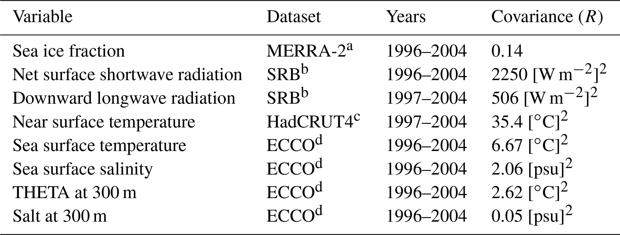
a GMAO (2016); bStackhouse et al. (2011); cOsborn and Jones (2014); dForget et al. (2015)
4.2 Observational targets
The motivation of this study was to set up a simple, systematic, reproducible, extensible, and efficient framework for improving the climatology of the new coupled model both now and as it undergoes development in the future. To start, we chose eight key observational targets (Table 1), each one chosen for the reasons outlined below. Ice fraction is directly relevant to all sea ice processes, and is important for an accurate representation of climate variability in the polar regions and climate feedbacks on the global scale. Accurate modeling of shortwave radiation at the surface indicates that the model can simulate the atmospheric and oceanic circulations' driving force. Shortwave radiation and downward longwave radiation indicate the realistic representation of cloud processes in the atmosphere. Near-surface temperature was added aiming to balance out ocean-only observational targets. Sea surface temperature (SST) is a fundamental climate variable that drives the atmosphere. Sea surface salinity (SSS) controls ocean circulation but is also a tracer of the global water cycle. Their equivalents at 300 m below sea level additionally constrain large-scale ocean transports. The observational targets were calculated separately for each season – DJF (December, January, February), MAM (March, April, May), JJA (June, July, August), SON (September, October, November) – and each seasonal mean was compared with the corresponding model output.
4.3 Definition of cost function
In this study, Q−1 is set to zero, i.e., the cost function does not explicitly include a priori knowledge about the range of possible parameter values. Some of the parameters, however, have intrinsic physical boundaries for the range of values. For these parameters, the resulting optimized parameters were checked and all were found to lie within the range of physically acceptable values. The error covariance matrix R is chosen to be diagonal. Because the estimation problem is highly overdetermined – the number of parameters to adjust is O(10) while the number of observations is O(106) – we expect that the assumption that R is diagonal will have minimal impact on the optimized estimate ηa. In general, the addition of non-diagonal elements of R would indicate linear dependence among observational errors, reducing the effective degrees of freedom. Since in our case the number of observations is far larger than the number of optimized parameters, we would still retain a very large number of independent observations as compared to optimized parameters. The variance was calculated separately for each observational target and defined to be the global, area-weighted, mean-squared difference between the climatology of the reference experiment and observations, that is
where the indices v, i, j, and s represent observation variable, longitude, latitude, and season (winter, spring, summer, and fall), the hat sign represents climatological seasonal mean values, and wi,j is an area weight with , giving each season a of the weight. The prior error variance of each variable is, therefore, a constant value. A consequence of our choice of the covariance matrix and the cost function is that the cost of the reference experiment is equal to one for each variable. For eight observational targets, the total cost of the reference experiment is eight. This definition gives equal weight to each of the eight observational targets and was found to provide a balanced solution in terms of each observational target's overall influence. The cost of the optimized experiment is expected to be smaller than one for each variable.
4.4 Sensitivity experiments
In addition to the reference experiment, 20 different 10-year sensitivity experiments were performed using the exact model configuration as the reference experiment but perturbing one of the uncertain parameters each time. The length of the simulations needed for the Green's functions optimization is related to the application of the model being optimized. For climate projection applications, where the long-term equilibrium of the model is paramount, it seems clear that longer simulations would be warranted in order to allow for model spin-up time. The primary application of the coupled model presented here is seasonal to decadal prediction, and so the optimization is done to include (ideally to minimize) the initial model drift.
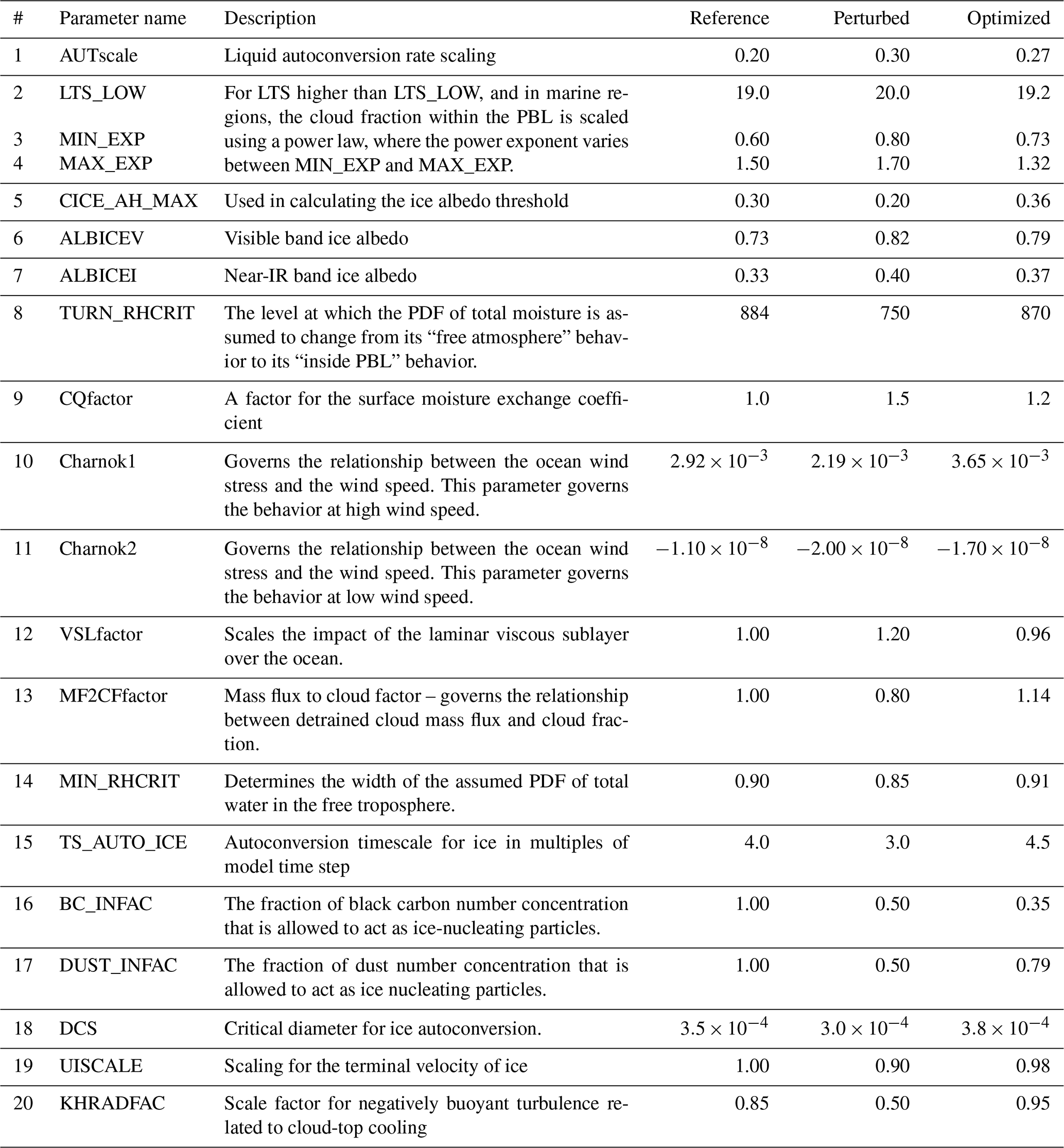
The reference and perturbed parameter values and a short description of the parameters are listed in Table 2. We used the 20 sensitivity experiments to estimate the model's sensitivity to each of the perturbed parameters based on the Green's functions formalism. The perturbed parameter values where chosen based on expert advice. For some of the parameters, the value was chosen based on physically realistic values from past experience. In some of the cases, the perturbed value was chosen arbitrarily due to a large parameter uncertainty. Note that there is no risk of overfitting due to the large number of observational targets (eight observational targets, two-dimensional fields, four seasons ≈300 000 targets). Methods to penalize a large number of parameters are therefore not needed in this case.
4.5 Optimized parameters
The optimized parameters are given in the last column of Table 2. It can be seen that only half of the optimized parameter values fall between the reference and the perturbed value, indicating a large unpredictability in model response to the change in those parameters. Nevertheless, the difference between the optimized parameter and the reference value (ηa) did not exceed the difference between the perturbed parameter value and the reference value (η), except for one parameter, i.e., TS_AUTO_ICE. This may indicate that our choice of the perturbed values was within a realistic range – particularly when considering that Q−1 was set to zero, suggesting that the optimized parameter's range was not constrained by the cost function.
4.6 Assessing the performance of the Green's functions methodology
Once the Green's functions methodology provides the optimized parameters, a projected cost can be derived directly from the sensitivity experiments using the optimized parameters. This derivation can be done before actually running the optimized simulation with the optimized parameters. The projected cost provides a first indication of the expected cost reduction, assuming linearity. After a new optimized experiment is performed, the projected cost can be compared with the optimized experiment's cost to assess the correctness of the assumption of linearity.
Figure 1 (and Table 3) shows that the total cost reduction of the optimized experiment (shown on the right) relative to the reference experiment (shown on the left) is 9 % (similar to the cost reduction found in Zhang et al. (2015)). Figure 1 (and Table 3) also shows the projected cost, which is the cost one would have if the model response to parameter perturbations were entirely linear. Most of the cost reduction seen in the projected (second from the right) experiment is realized in the optimized experiment. The total cost of each of the 20 sensitivity experiments is larger than the cost of the simulation with the optimized parameters. Figure 2 shows the normalized cost for each of the eight observational targets in the same order as in Fig. 1. Figure 2 shows that the cost is lowest in the optimized experiment (the rightmost bar in each cluster) for five out of the eight observational targets. For one of the observational targets (sea ice fraction), the cost of the optimized experiment is smaller than the reference but several sensitivity experiments have lower cost. For two observational targets, the optimized experiment cost is higher than the cost of the reference experiment. This cost increase happens for surface temperature over land and downward longwave radiation. The longwave radiation had a cost increase of 2 %. The more considerably increased cost of 16 % in the surface temperature is related to our choice of observational targets. Five out of the eight observational targets are ocean-only variables, only one is land-only, and two cover both land and ocean. This asymmetry between land and ocean constraints seems to have pulled the parameters to values that benefit the ocean more than the land. The proof of concept illustrated in this study, although clearly demonstrating the overall cost reduction with this method, also illustrates the need to choose the desired observational targets carefully.
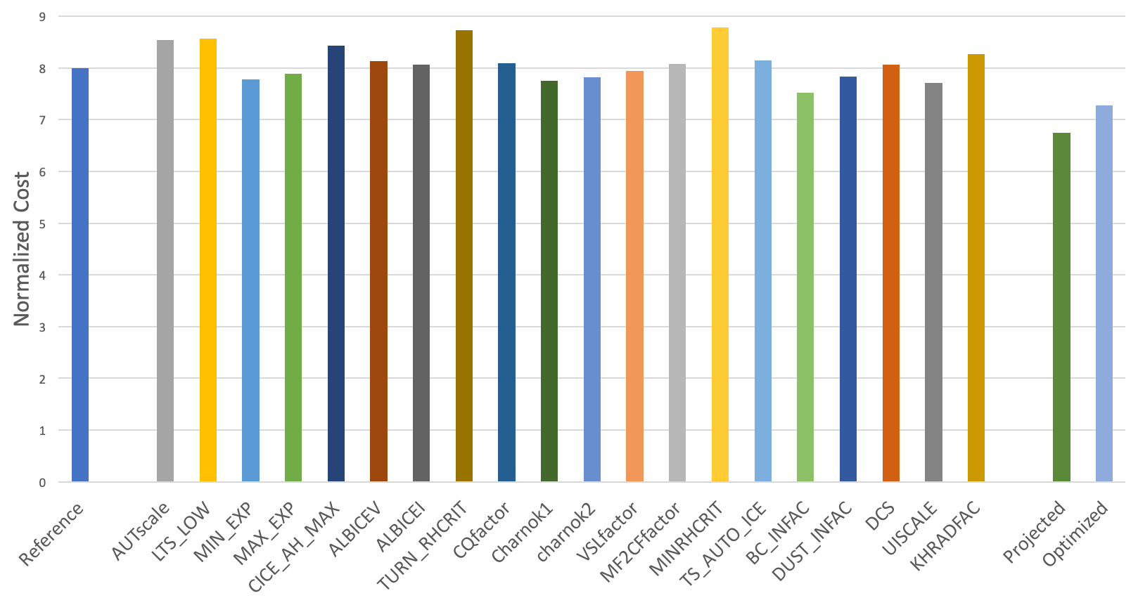
Figure 1The total cost of the reference experiment, the optimized experiment, and the 20 perturbed experiments. Projected cost is also indicated.
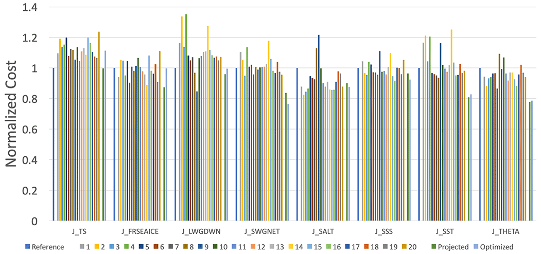
Figure 2The cost of the reference experiment and the 20 perturbed experiments for each of the observational targets. Projected and optimized costs are also indicated.
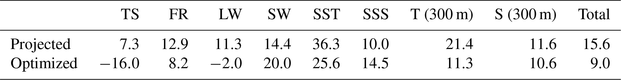
Table 3Explained variance in percentage. Negative values represent reduction of explained variance. TS: near-surface temperature; FR: sea ice fraction; LW: downward longwave radiation; SW: net surface shortwave radiation; SST: sea surface temperature; SSS: sea surface salinity; T (300): THETA at 300 m; S (300): salt at 300 m.
The cost reduction was also found to be rather homogeneous across many regions around the globe. Figure 3 shows that for net shortwave radiation, the total cost reduction was 20 % relative to the reference experiment. Most of the oceans exhibit a large reduction in the cost, particularly over the Antarctic Circumpolar Current (ACC) and in the stratocumulus regions in the eastern Pacific's subtropics. In comparison with these cost reductions over the oceans, the land still exhibits marginal increases in cost over wide regions of North America and Southeast Asia.
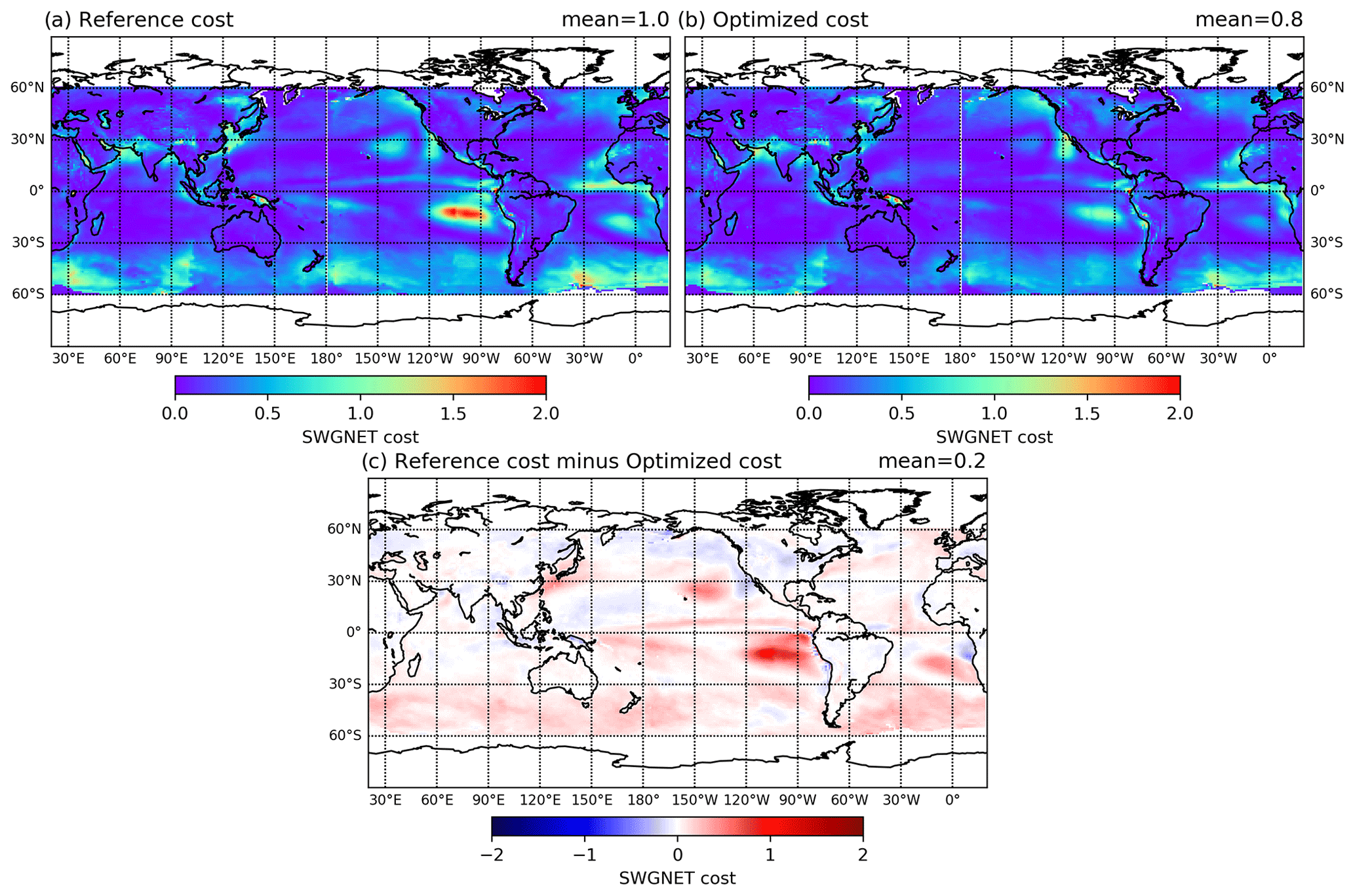
Figure 3The net shortwave radiation cost for the reference (a), the optimized experiments (b), and their difference (c).
The actual cost reduction of the various variables seen in the optimized experiment is also generally consistent with the projected cost. Figure 4 shows the projected cost reduction for the net shortwave radiation, which is in broad agreement with the actual cost reduction of the optimized experiment seen in Fig. 3c. In this case, the cost of the optimized experiment was even smaller than the projected cost. Overall agreement between the projected cost and optimized experiment cost suggests that the linearity assumption that underlies the Green's functions methodology holds sufficiently well for the approach to be useful.
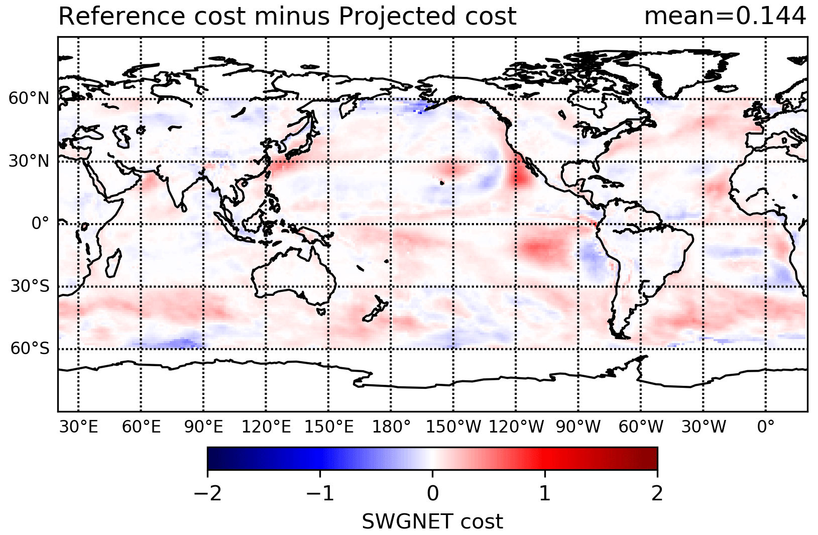
Figure 4Net shortwave radiation cost difference between the projected value and the reference experiment.
The surface temperature, which exhibits an overall 16 % increase in cost (Fig. 5), also shows some large regions of cost reduction over North America and Greenland. However, the cost in North Asia and Europe is increased. In terms of the cost's seasonality, it was found that DJF and MAM had the highest cost increase, while JJA months had the smallest overall cost reductions. These results suggest that the misrepresentation of land ice processes in the new and the old configurations is responsible for the high cost. Surface temperature is the variable that had the least projected cost reduction; thus, it was expected to exhibit the worst performance in terms of the optimized experiment cost. Including more land-related observational targets, such as snow fraction and soil moisture, could improve the cost of surface temperature. This inclusion can assist in constraining model performance above land, balancing the ocean-only constraints. Downward longwave radiation also exhibits cost increase, but here the increase is 2 %. In terms of the other variables, the cost of sea ice fraction was reduced by 8.2 %, and the four ocean-only variables showed cost reduction between 10 and 25 %, indicating an improved representation of the ocean circulation.
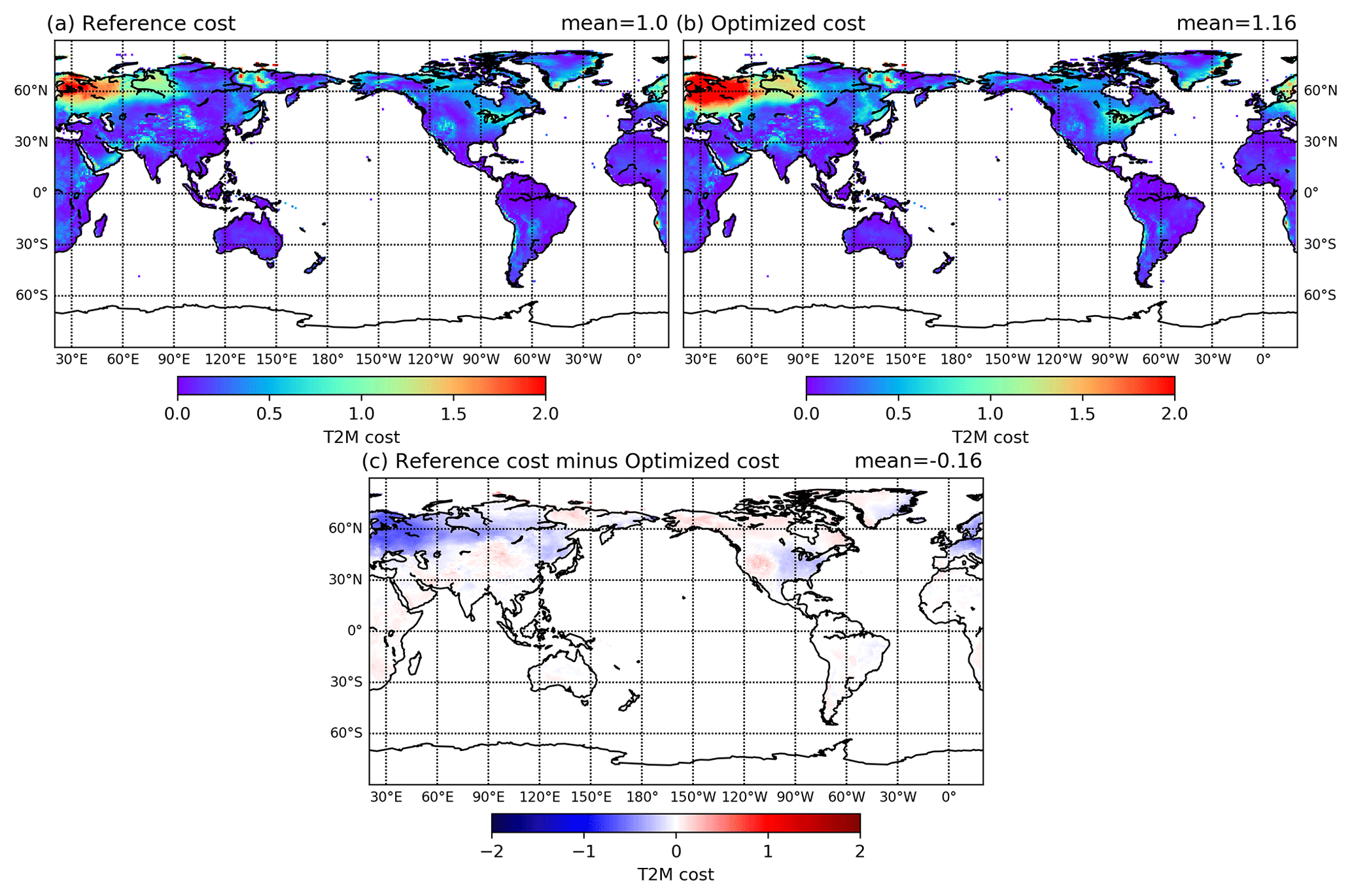
Figure 5The 2 m temperature cost for the reference (a) and the optimized experiments (b), and their difference (c).
The parameter estimation experiment presented in the previous section describes our current best practice, which was guided by a series of sensitivity experiments with different configurations, where different variations of the methodology were tested. Below, we discuss sensitivity to the choice of (1) prior covariance matrices, (2) observational targets, and (3) the number of control parameters. Many other sensitivity experiments can be designed. The goal of this section is not to cover all the options, but rather to provide an additional dimensional depth of the Green's functions methodology. In the end, the future choice of the Green's functions “flavor” should reflect the goals of the optimization exercise.
5.1 Sensitivity to choice of prior covariance matrices
In general, the error covariance matrices Q and R are not known and difficult to estimate. For the Green's functions approach, however, the number of observations is generally much larger than the number of parameters being estimated, which simplifies the selection of Q and R. First, the small number of control parameters limits the solution's degrees of freedom; therefore, the choice of Q and R, if they are reasonable, is not expected to change the solution ηa much – but it will impact posterior uncertainty, P. Second, the data kernel matrix G is small enough to be defined explicitly; therefore, many interesting properties of the solution can be derived and evaluated. Third, the solution of Eqs. (8) and (9), once the kernel matrix G has been derived, is trivial; therefore, it is possible to test the impact of particular choices of Q and R, as is done next.
The sensitivity to the choice of covariance matrices Q and R in Eq. (4) is evaluated using a pared-down configuration, perturbing only three parameters. The pared-down configuration is used to simplify the discussion and better illustrate the response of the optimized solution to different covariance matrices. The perturbed parameters were AUTscale, LTS_LOW, and two sea ice parameters (ALBICEV and ALBICEI) perturbed together. The output from the methodology for this choice is a set of scaling factors for the parameters. When more than one parameter is perturbed in one experiment, the same scaling factor is applied to all the experiment parameters. In this configuration, unlike in our best-practice configuration, the observational targets were multi-year means, and the cost was not computed separately for each season. The observational targets are also similar to the best-practice configuration, except that the 500 mbar height was used in place of the surface temperature over land, and the net radiation replaced the two radiation components.
We tested four different options for the prior error variance, the diagonal elements of matrix R:
where, are the variable, longitude, latitude, season, time indexes, respectively. The tilde symbol () represents seasonal means and N is the number of years. The first option (a) uses the area-weighted variance of the observations instead of the mean-squared misfits used in Eq. (10). The second option (b) is the spatially and seasonally variable time variance of the observations, the third option (c) is the square of the maximal absolute difference between observations and the reference experiment, and the fourth option (d) is an area-weighted variance of the difference between the observations and the reference experiment. All four estimates of R are calculated separately for each variable. The four estimates of R aim to represent a range of plausible estimates for the actual error variance and allow us to explore the effect on the resulting parameters and cost.
We calculated optimized parameters, ηa, for each of the four definitions of R assuming that Q=∞, i.e., no prior information about the control parameters, and again assuming that Q=I, the identity matrix, meaning that we have the same amount of confidence in the prior values of each control parameter. These two estimates of Q represent two extreme situations.
Table 4 shows the eight different combinations of the parameters based on the four options for the observations' covariance and two different parameters governing the covariance matrices. In general, all configurations generate realistic values in terms of the order of magnitude, but parameters differ in detail. The Q=I case tends to keep parameters closer to their initial value (relative to Q=∞), as expected.
Table 5 shows the cost associated with each of the eight experiments. Looking at the Q=∞ cases, defining the cost based on Eq. (11a) reduced the cost by 7.7 % but the relative importance of each variable varied substantially. For example, 500 mbar height cost was very small for the reference (0.024) and the fact that the optimized experiment increased the cost by 33.7 % did not affect the total cost. Also, the sea ice contribution to the cost was much larger than the temperature and salinity at 300 m below the sea surface. Option (11b) was found to provide only marginal cost reduction. Option (11c) demonstrated the largest cost reduction (the smallest ratio in the J_total column). However, most of the projected cost reduction was restricted to the 500 mbar height target, while the cost of most of the other variables was not reduced, particularly in the case of the ocean targets. This is in contrast with option (11d), for which the cost reduction was spread more uniformly across the observational targets. All of these considerations led to our choice of option (11d) as the best practice. The Q=I was not chosen because the range of the parameters is in itself often quite uncertain and because optimized parameter values were found to remain reasonable without the need for adding this additional constraint to the cost function. This choice is certainly worth revisiting in a future study.
After running a new model simulation with the optimized parameters based on Eq. (11d) and the Q=∞ case, the total cost reduction was found to be 6 % – 2.9 % less than the projected value, but still not small (Table 5). The 500 mbar height contributes to most of the reduction, and the sea ice cost was increased by about 25 %. A possible explanation for the 500 mbar target being the main contributor to the cost reduction is that there were a small number of grid points in which the error was reduced substantially, particularly at high latitudes (not shown). This result suggests an experiment in which a spatially dependent weight is used to reduce the magnitude of the outliers. The current cost implementation has dependency on the model squared error. This dependency favors the correction of a small number of points with large errors relative to a large number of points with small errors. Choosing absolute error instead of squared error would have changed the tendency to favor the correction of a small number of grid points with large errors. Nevertheless, the simpler experiment configuration was a successful choice to explore the sensitivity to the covariance matrix designs.
Table 4Optimized parameters of the three perturbed parameters experiments based on two different definitions of the parameters' covariance matrix Q and four definitions of the error covariance matrix (Eq. 11a–11d).


5.2 Sensitivity to choice of number of parameters
Here, we evaluate the sensitivity of the cost to the number of optimized parameters. We calculated the projected cost reduction for four cases which used a subset of the first 5, 10, 15, and all 20 parameters from Table 2. We focus here on an optimization based on the multi-year means. An increased number of parameters is expected to translate into a reduced cost as we fit the model to more parameters. In the following results, we decided to remove the 500 mbar height from the cost function in order to spread the cost across more variables. Generally, there is nothing wrong with having most of the cost reduced in one of the observational targets, but we decided here to seek a more balanced cost reduction. An additional change here and in the following sections is the separation of the net surface radiation target into net shortwave and downward longwave radiation, as they are independent and both have SRB (surface radiation budget) observational counterparts. The choice of downward longwave radiation rather than the net was made due to the direct dependence of upward longwave radiation on the SST (which is already a constraint).
We tested the projected cost reduction as a function of the optimized parameter number (Fig. 6). We found that the projected cost was reduced from 6 to 25 % when going from 5 optimized parameters to 20. The cost reduction was gradual, showing an additional reduction with the increase of the optimized parameters. The largest cost reduction was found between 5 and 10 optimized parameters.
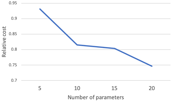
Figure 6Cost relative to the reference experiment as a function of the number of optimized parameters based on annual means.
5.3 Annual mean versus seasonal mean data constraints
Here, we used nine sensitivity experiments, with nine optimized parameters, to look at the sensitivity of the optimized parameters to seasonality. Two sets of parameters were calculated based on multi-year means (annual, Table 6) and based on multi-year seasonal means (seasonal, Table 6). Calculation of the optimized parameters comes after performance of the simulations, so the input simulations are the same for both options. The only difference between the annual and seasonal suites is the configuration of the cost function provided to the Greens' functions methodology.
The most noteworthy difference between the annual and seasonal results was found in the Charnock parameter that controls surface winds. Although the difference between parameters is smaller than 10 %, the projected cost differences are large, with the annually based optimization reducing the cost by about 15 % and the seasonally based optimization reducing the cost by about 9 %. This result is expected, as seasonally based data have more variability and we use the same number of parameters to optimize model results to a larger number of observations.
Optimizing for seasonal observational targets is expected to be essential for improving seasonal variability. Therefore, despite the less efficient cost reduction for the seasonal targets, we decided to continue to focus on experiments with seasonal observational targets. For these two sets of experiments, we did not choose to rerun the model with optimized parameters, but instead decided to increase the number of optimized parameters by performing additional simulations.
Table 6Optimized parameters of the nine perturbed parameters experiments configured with Q=∞ and option (11d).
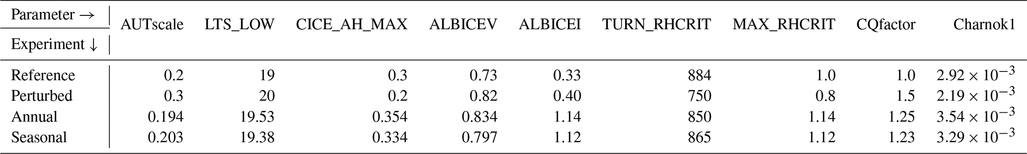
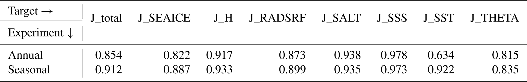
Table 7Proj./ref. cost of the nine perturbed parameters experiment configured with Q=∞ and option (11d).
5.4 Length of the optimization period
This sensitivity test was performed with the 20-parameter set of simulations. The appropriate length of the sensitivity experiments was chosen based on the intended application of our tuned model for seasonal and decadal prediction. It seems clear that for a different application of the model, say climate projection, the length of the sensitivity experiments, optimization, and observational targets must be long enough to reach a climate equilibrium. Within the scope of seasonal to decadal prediction, to examine the impact of the optimization period, we performed three Green's function calculations: one that optimizes the parameters based on the first 5 years of the runs (2000–2005), one that uses the last 5 years of the runs (2005–2010), and another that uses the whole 10 years (2000–2010) as in Sect. 4. The motivation here was to learn about the impact of model drift after initialization on the optimization. The 2000–2005 optimization projected a 15.3 % cost reduction, the 2005–2010 optimization projected a 12.4 % cost reduction, and the 2000–2010 optimization projected a 15.6 % cost reduction. The optimized experiments were only performed with the total and latter time period optimization results, and the 2005–2010 optimized parameters had a cost reduction of 7.1 % relative to 9 % for the 2000–2010 experiment. One of the plausible reasons for less cost reduction when optimizing the latter period only is that 2005–2010 had fewer than two El Niño cycles, and it was too short for the calculation of the model climatology. The 10-year experiment had three full El Niño cycles, and its climatology represents the model climatology more adequately. The 10-year optimization, therefore, is found to enable better parameter optimization.
This study demonstrates the applicability of the Green's functions approach – introduced in Menemenlis et al. (2005) for a forced ocean simulation – to the adjustment of uncertain parameters for a coupled ocean—atmosphere simulation. In this proof-of-concept study, we computed the response of the coupled ocean–atmosphere simulation to the perturbation of the 20 parameters listed in Table 1. These 20 perturbation experiments were subsequently used to optimize the values of the 20 parameters. The observational targets were long-term seasonal means of the eight fields listed in Table 2. The optimization increased the explained variance by up to 25 % (for SST in Table 3).
The Green's functions approach assumes that the response of the model to small perturbations is approximately linear. This assumption does not rigorously hold for atmospheric, oceanic, or coupled ocean–atmosphere models because of nonlinear weather and climate phenomena such as synoptic storms and El Niño–Southern Oscillation (ENSO) variability. Therefore, a key consideration is that the perturbation experiments be sufficiently long to average out nonlinear weather and lower-frequency phenomena. This study shows that 10-year long simulations can be sufficient to enable successful application of the Green's functions approach.
The cost reduction was spread across most of the observational targets, though our configuration of observational targets may have been responsible for the cost increase in two amongst them – the targets associated with land areas that are underrepresented in our cost function. In the end, the choice of the observational targets should reflect the objective of the study and, probably, there is no single set of observational targets that is adequate for all applications a priori. Our proof-of-concept study and the experiments that show the impact of different choices in the details readily reflect the tradeoffs among data constraints that can be important considerations.
Increasing the number of optimized parameters reduced the overall cost, an effect which seems to be quasi-linear with the number of parameters, but further investigation into this is required. Increasing the temporal resolution of the observational targets from annual to seasonal increased the cost further – a result of the increasing number of observational targets. Adding seasonality into parameter adjustments is viewed as one of the next logical steps in this regard. We also tested four different methods to calculate the error covariance matrix, and found that using the error of the reference experiment produced the most balanced results in terms of accounting for all observational targets.
This study shows that the Green's functions methodology can benefit the earth system modeling community by providing a more structured yet practical method to tune the complex global models. The Green's functions methodology has several advantages that are worth emphasizing here: (a) it is simple to implement and it does not require internal amendments to the model code; (b) it is relatively cheap for a small number of parameters – one extra sensitivity experiment per parameter; (c) one can generate virtual predictions and calculate projected cost for a very large number of cost configurations without running new experiments; (d) it offers a systematic way to optimize parameters accounting for a possible dependent response of the model to a change of different parameters; (e) the optimization process can be extended with more sensitivity experiments and it can also be revisited with a different set of parameters; and (f) the sensitivity experiments can be done in parallel, suggesting potential scalability.
Identifying the most important uncertain parameters for applying Green's functions methodology still requires close familiarity with models and there is no replacement for the experience of the modelers when using this methodology. Therefore it is viewed as a valuable framework to further leverage modelers' expertise to fine-tune model parameters, standardize practices across the various modeling centers, and improve model products beyond the present state of the art.
Data leading to this publication were made available as part of a Zenodo repository at https://doi.org/10.5281/zenodo.5507631 (Strobach, 2021). This repository includes models' code and configuration files, postprocessed data from model simulations and observational targets, and Green's functions-related scripts, including those generating the figures and tables.
ES ran the simulation and performed the experiments. AM, DB, AT, DM, and GF contributed to the design of the experiments and writing the manuscript.
The contact author has declared that neither they nor their coauthors have any competing interests.
Publisher's note: Copernicus Publications remains neutral with regard to jurisdictional claims in published maps and institutional affiliations.
The SRB data were obtained from the NASA Langley Research Center Atmospheric Sciences Data Center NASA/GEWEX SRB Project. This research was made possible by grants from the NASA Modeling, Analysis, and Prediction (MAP) and Physical Oceanography (PO) programs. GEOS development was funded under NASA MAP-supported GMAO “core” funding. Dimitris Menemenlis carried out research at the Jet Propulsion Laboratory, California Institute of Technology, under contract with NASA. High-end computing resources were provided by the NASA Center for Climate Simulation (NCCS).
This paper was edited by Fabien Maussion and reviewed by two anonymous referees.
Adcroft, A. and Campin, J.-M.: Rescaled height coordinates for accurate representation of free-surface flows in ocean circulation models, Ocean Model., 7, 269–284, https://doi.org/10.1016/j.ocemod.2003.09.003, 2004. a, b
Danabasoglu, G., Lamarque, J.-F., Bacmeister, J., Bailey, D. A., DuVivier, A. K., Edwards, J., Emmons, L. K., Fasullo, J., Garcia, R., Gettelman, A., Hannay, C., Holland, M. M., Large, W. G., Lauritzen, P. H., Lawrence, D. M., Lenaerts, J. T. M., Lindsay, K., Lipscomb, W. H., Mills, M. J., Neale, R., Oleson, K. W., Otto-Bliesner, B., Phillips, A. S., Sacks, W., Tilmes, S., van Kampenhout, L., Vertenstein, M., Bertini, A., Dennis, J., Deser, C., Fischer, C., Fox-Kemper, B., Kay, J. E., Kinnison, D., Kushner, P. J., Larson, V. E., Long, M. C., Mickelson, S., Moore, J. K., Nienhouse, E., Polvani, L., Rasch, P. J., and Strand, W. G.: The Community Earth System Model Version 2 (CESM2), J. Adv. Model. Earth Sy., 12, e2019MS001916, https://doi.org/10.1029/2019MS001916, 2020. a
Forget, G., Campin, J.-M., Heimbach, P., Hill, C. N., Ponte, R. M., and Wunsch, C.: ECCO version 4: an integrated framework for non-linear inverse modeling and global ocean state estimation, Geosci. Model Dev., 8, 3071–3104, https://doi.org/10.5194/gmd-8-3071-2015, 2015. a, b, c
Garfinkel, C. I., Molod, A. M., Oman, L. D., and Song, I.-S.: Improvement of the GEOS-5 AGCM upon updating the air-sea roughness parameterization, Geophys. Res. Lett., 38, L18702, https://doi.org/10.1029/2011GL048802, l18702, 2011. a
GMAO: Global Modeling and Assimilation Office, MERRA-2 tavg1_2d_ocn_Nx: 2d, 1-Hourly, Time-Averaged, Single-Level, Assimilation, Ocean Surface Diagnostics V5.12.4, Goddard Earth Sciences Data and Information Services Center (GES DISC), Greenbelt, MD, USA, https://doi.org/10.5067/Y67YQ1L3ZZ4R, 2016. a
Golaz, J.-C., Caldwell, P. M., Van Roekel, L. P., Petersen, M. R., Tang, Q., Wolfe, J. D., Abeshu, G., Anantharaj, V., Asay-Davis, X. S., Bader, D. C., Baldwin, S. A., Bisht, G., Bogenschutz, P. A., Branstetter, M., Brunke, M. A., Brus, S. R., Burrows, S. M., Cameron-Smith, P. J., Donahue, A. S., Deakin, M., Easter, R. C., Evans, K. J., Feng, Y., Flanner, M., Foucar, J. G., Fyke, J. G., Griffin, B. M., Hannay, C., Harrop, B. E., Hoffman, M. J., Hunke, E. C., Jacob, R. L., Jacobsen, D. W., Jeffery, N., Jones, P. W., Keen, N. D., Klein, S. A., Larson, V. E., Leung, L. R., Li, H.-Y., Lin, W., Lipscomb, W. H., Ma, P.-L., Mahajan, S., Maltrud, M. E., Mametjanov, A., McClean, J. L., McCoy, R. B., Neale, R. B., Price, S. F., Qian, Y., Rasch, P. J., Reeves Eyre, J. E. J., Riley, W. J., Ringler, T. D., Roberts, A. F., Roesler, E. L., Salinger, A. G., Shaheen, Z., Shi, X., Singh, B., Tang, J., Taylor, M. A., Thornton, P. E., Turner, A. K., Veneziani, M., Wan, H., Wang, H., Wang, S., Williams, D. N., Wolfram, P. J., Worley, P. H., Xie, S., Yang, Y., Yoon, J.-H., Zelinka, M. D., Zender, C. S., Zeng, X., Zhang, C., Zhang, K., Zhang, Y., Zheng, X., Zhou, T., and Zhu, Q.: The DOE E3SM Coupled Model Version 1: Overview and Evaluation at Standard Resolution, J. Adv. Model. Earth Sy., 11, 2089–2129, https://doi.org/10.1029/2018MS001603, 2019. a
Helfand, H. M. and Schubert, S. D.: Climatology of the Simulated Great Plains Low-Level Jet and Its Contribution to the Continental Moisture Budget of the United States, J. Climate, 8, 784–806, https://doi.org/10.1175/1520-0442(1995)008<0784:COTSGP>2.0.CO;2, 1995. a
Hourdin, F., Mauritsen, T., Gettelman, A., Golaz, J.-C., Balaji, V., Duan, Q., Folini, D., Ji, D., Klocke, D., Qian, Y., Rauser, F., Rio, C., Tomassini, L., Watanabe, M., and Williamson, D.: The Art and Science of Climate Model Tuning, B. Am. Meteorol. Soc., 98, 589–602, https://doi.org/10.1175/BAMS-D-15-00135.1, 2017. a
Hunke, E. and Lipscomb, W.: CICE: The Los Alamos sea ice model documentation and software user's manual version 4.0 LA-CC-06-012, Tech. Rep. LA-CC-06-012, http://www.ccpo.odu.edu/~klinck/Reprints/PDF/cicedoc2015.pdf (last access: 15 March 2022), 2010. a
Kalnay, E.: Atmospheric Modeling, Data Assimilation and Predictability, Cambridge University Press, https://doi.org/10.1017/CBO9780511802270, 2002. a
Large, W. G., McWilliams, J. C., and Doney, S. C.: Oceanic vertical mixing: A review and a model with a nonlocal boundary layer parameterization, Rev. Geophys., 32, 363–403, https://doi.org/10.1029/94RG01872, 1994. a
Marshall, J., Adcroft, A., Hill, C., Perelman, L., and Heisey, C.: A finite-volume, incompressible Navier Stokes model for studies of the ocean on parallel computers, J. Geophys. Res.-Oceans, 102, 5753–5766, https://doi.org/10.1029/96JC02775, 1997. a
Mauritsen, T., Stevens, B., Roeckner, E., Crueger, T., Esch, M., Giorgetta, M., Haak, H., Jungclaus, J., Klocke, D., Matei, D., Mikolajewicz, U., Notz, D., Pincus, R., Schmidt, H., and Tomassini, L.: Tuning the climate of a global model, J. Adv. Model. Earth Sy., 4, M00A01, https://doi.org/10.1029/2012MS000154, 2012. a
Mauritsen, T., Bader, J., Becker, T., Behrens, J., Bittner, M., Brokopf, R., Brovkin, V., Claussen, M., Crueger, T., Esch, M., Fast, I., Fiedler, S., Fläschner, D., Gayler, V., Giorgetta, M., Goll, D. S., Haak, H., Hagemann, S., Hedemann, C., Hohenegger, C., Ilyina, T., Jahns, T., Jimenéz-de-la Cuesta, D., Jungclaus, J., Kleinen, T., Kloster, S., Kracher, D., Kinne, S., Kleberg, D., Lasslop, G., Kornblueh, L., Marotzke, J., Matei, D., Meraner, K., Mikolajewicz, U., Modali, K., Möbis, B., Müller, W. A., Nabel, J. E. M. S., Nam, C. C. W., Notz, D., Nyawira, S.-S., Paulsen, H., Peters, K., Pincus, R., Pohlmann, H., Pongratz, J., Popp, M., Raddatz, T. J., Rast, S., Redler, R., Reick, C. H., Rohrschneider, T., Schemann, V., Schmidt, H., Schnur, R., Schulzweida, U., Six, K. D., Stein, L., Stemmler, I., Stevens, B., von Storch, J.-S., Tian, F., Voigt, A., Vrese, P., Wieners, K.-H., Wilkenskjeld, S., Winkler, A., and Roeckner, E.: Developments in the MPI-M Earth System Model version 1.2 (MPI-ESM1.2) and Its Response to Increasing CO2, J. Adv. Model. Earth Sy., 11, 998–1038, https://doi.org/10.1029/2018MS001400, 2019. a
Menemenlis, D., Fukumori, I., and Lee, T.: Using Green's Functions to Calibrate an Ocean General Circulation Model, Mon. Weather Rev., 133, 1224–1240, https://doi.org/10.1175/MWR2912.1, 2005. a, b
Molod, A., Suarez, M., and Partyka, G.: The impact of limiting ocean roughness on GEOS-5 AGCM tropical cyclone forecasts, Geophys. Res. Lett., 40, 411–416, https://doi.org/10.1029/2012GL053979, 2013. a
Molod, A., Hackert, E., Vikhliaev, Y., Zhao, B., Barahona, D., Vernieres, G., Borovikov, A., Kovach, R. M., Marshak, J., Schubert, S., Li, Z., Lim, Y.-K., Andrews, L. C., Cullather, R., Koster, R., Achuthavarier, D., Carton, J., Coy, L., Friere, J. L. M., Longo, K. M., Nakada, K., and Pawson, S.: GEOS-S2S Version 2: The GMAO High-Resolution Coupled Model and Assimilation System for Seasonal Prediction, J. Geophys. Res.-Atmos., 125, e2019JD031767, https://doi.org/10.1029/2019JD031767, 2020. a
Osborn, T. J. and Jones, P. D.: The CRUTEM4 land-surface air temperature data set: construction, previous versions and dissemination via Google Earth, Earth Syst. Sci. Data, 6, 61–68, https://doi.org/10.5194/essd-6-61-2014, 2014. a
Posselt, D., Fryxell, B., Molod, A., and Williams, B.: Quantitative Sensitivity Analysis of Physical Parameterizations for Cases of Deep Convection in the NASA GEOS-5 Model, J. Climate, 29, 151029073005006, https://doi.org/10.1175/JCLI-D-15-0250.1, 2015. a, b
Price, J. F., Mooers, C. N. K., and Van Leer, J. C.: Observation and Simulation of Storm-Induced Mixed-Layer Deepening, J. Phys. Oceanogr., 8, 582–599, https://doi.org/10.1175/1520-0485(1978)008<0582:OASOSI>2.0.CO;2, 1978. a
Roach, L. A., Tett, S. F., Mineter, M. J., Yamazaki, K., and Rae, C. D.: Automated parameter tuning applied to sea ice in a global climate model, Clim. Dynam., 50, 51–65, 2018. a
Schmidt, G. A., Bader, D., Donner, L. J., Elsaesser, G. S., Golaz, J.-C., Hannay, C., Molod, A., Neale, R. B., and Saha, S.: Practice and philosophy of climate model tuning across six US modeling centers, Geosci. Model Dev., 10, 3207–3223, https://doi.org/10.5194/gmd-10-3207-2017, 2017. a
Sellar, A. A., Jones, C. G., Mulcahy, J. P., Tang, Y., Yool, A., Wiltshire, A., O'Connor, F. M., Stringer, M., Hill, R., Palmieri, J., Woodward, S., de Mora, L., Kuhlbrodt, T., Rumbold, S. T., Kelley, D. I., Ellis, R., Johnson, C. E., Walton, J., Abraham, N. L., Andrews, M. B., Andrews, T., Archibald, A. T., Berthou, S., Burke, E., Blockley, E., Carslaw, K., Dalvi, M., Edwards, J., Folberth, G. A., Gedney, N., Griffiths, P. T., Harper, A. B., Hendry, M. A., Hewitt, A. J., Johnson, B., Jones, A., Jones, C. D., Keeble, J., Liddicoat, S., Morgenstern, O., Parker, R. J., Predoi, V., Robertson, E., Siahaan, A., Smith, R. S., Swaminathan, R., Woodhouse, M. T., Zeng, G., and Zerroukat, M.: UKESM1: Description and Evaluation of the U.K. Earth System Model, J. Adv. Model. Earth Sy., 11, 4513–4558, https://doi.org/10.1029/2019MS001739, 2019. a
Stackhouse Jr., P. W., Gupta, S. K., Cox, S. J., Zhang, T., Mikovitz, J. C., and Hinkelman, L. M.: The NASA/GEWEX surface radiation budget release 3.0: 24.5-year dataset, Gewex news, 21, 10–12, 2011. a
Strobach, E.: Data for the paper: Earth System Model Parameter Adjustment Using a Green's Functions Approach (Version v1), Zenodo [code/data set], https://doi.org/10.5281/zenodo.5507631, 2021. a
Tett, S. F., Mineter, M. J., Cartis, C., Rowlands, D. J., and Liu, P.: Can top-of-atmosphere radiation measurements constrain climate predictions? Part I: Tuning, J. Climate, 26, 9348–9366, 2013. a
Tett, S. F. B., Yamazaki, K., Mineter, M. J., Cartis, C., and Eizenberg, N.: Calibrating climate models using inverse methods: case studies with HadAM3, HadAM3P and HadCM3, Geosci. Model Dev., 10, 3567–3589, https://doi.org/10.5194/gmd-10-3567-2017, 2017. a
Voldoire, A., Saint-Martin, D., Sénési, S., Decharme, B., Alias, A., Chevallier, M., Colin, J., Guérémy, J.-F., Michou, M., Moine, M.-P., Nabat, P., Roehrig, R., Salas y Mélia, D., Séférian, R., Valcke, S., Beau, I., Belamari, S., Berthet, S., Cassou, C., Cattiaux, J., Deshayes, J., Douville, H., Ethé, C., Franchistéguy, L., Geoffroy, O., Lévy, C., Madec, G., Meurdesoif, Y., Msadek, R., Ribes, A., Sanchez-Gomez, E., Terray, L., and Waldman, R.: Evaluation of CMIP6 DECK Experiments With CNRM-CM6-1, J. Adv. Model. Earth Sy., 11, 2177–2213, https://doi.org/10.1029/2019MS001683, 2019. a
Watanabe, M., Suzuki, T., O’ishi, R., Komuro, Y., Watanabe, S., Emori, S., Takemura, T., Chikira, M., Ogura, T., Sekiguchi, M., Takata, K., Yamazaki, D., Yokohata, T., Nozawa, T., Hasumi, H., Tatebe, H., and Kimoto, M.: Improved Climate Simulation by MIROC5: Mean States, Variability, and Climate Sensitivity, J. Climate, 23, 6312–6335, https://doi.org/10.1175/2010JCLI3679.1, 2010. a
Yukimoto, S., Adachi, Y., Hosaka, M., Sakami, T., Yoshimura, H., Hirabara, M., Tanaka, T., Shindo, E., Tsujino, H., Deushi, M., Mizuta, R., Yabu, S., Obata, A., Nakano, H., Koshiro, T., Ose, T., and Kitoh, A.: A New Global Climate Model of the Meteorological Research Institute: MRI-CGCM3, J. Meteorol. Soc. Japan, 90A, 23–64, https://doi.org/10.2151/jmsj.2012-A02, 2012. a
Zhang, T., Li, L., Lin, Y., Xue, W., Xie, F., Xu, H., and Huang, X.: An automatic and effective parameter optimization method for model tuning, Geosci. Model Dev., 8, 3579–3591, https://doi.org/10.5194/gmd-8-3579-2015, 2015. a, b
Zou, L., Qian, Y., Zhou, T., and Yang, B.: Parameter Tuning and Calibration of RegCM3 with MIT–Emanuel Cumulus Parameterization Scheme over CORDEX East Asia Domain, J. Climate, 27, 7687–7701, https://doi.org/10.1175/JCLI-D-14-00229.1, 2014. a
- Abstract
- Introduction
- Earth system model description
- Mathematical formalism and methodology
- Proof of concept optimization
- Discussion: motivation for choices in methodology
- Summary and Concluding Remarks
- Code and data availability
- Author contributions
- Competing interests
- Disclaimer
- Acknowledgements
- Review statement
- References