Empirical Lagrangian parametrization for wind-driven mixing of buoyant particles at the ocean surface

Turbulent mixing is a vital component of vertical particulate transport, but ocean global circulation models (OGCMs) generally have low-resolution representations of near-surface mixing. Furthermore, turbulence data are often not provided in OGCM model output. We present 1D parametrizations of wind-driven turbulent mixing in the ocean surface mixed layer that are designed to be easily included in 3D Lagrangian model experiments. Stochastic transport is computed by Markov-0 or Markov-1 models, and we discuss the advantages and disadvantages of two vertical profiles for the vertical diffusion coefficient K_z. All vertical diffusion profiles and stochastic transport models lead to stable concentration profiles for buoyant particles, which for particles with rise velocities of 0.03 and 0.003 m s⁻¹ agree relatively well with concentration profiles from field measurements of microplastics when Langmuir-circulation-driven turbulence is accounted for. Markov-0 models provide good model performance for integration time steps of Δt≈30 s and can be readily applied when studying the behavior of buoyant particulates in the ocean. Markov-1 models do not consistently improve model performance relative to Markov-0 models and require an additional parameter that is poorly constrained.

1 Introduction

Lagrangian models are essential tools to examine the transport of particulates in the ocean on a variety of spatial and temporal scales (Van Sebille et al., 2018) and have been used to study the movement of plastic particulates (Onink et al., 2019), oil (Samaras et al., 2014) and fish larvae (Paris et al., 2013). However, especially in the field of marine plastic modeling, most large-scale modeling studies consider only virtual particles (henceforth referred to as particles) that float and remain at the ocean surface (Lebreton et al., 2018; Liubartseva et al., 2018; Onink et al., 2019, 2021), essentially simplifying the three-dimensional ocean into a 2D system. While this does reduce the complexity of models, ultimately vertical transport processes need to be considered in order to have a complete understanding of oceanic particulate transport (Wichmann et al., 2019; Van Sebille et al., 2020).

In the case of buoyant particulates (particulates with a density lower than seawater), buoyancy is expected to return any particulates to the ocean surface. However, instead of all buoyant particulates accumulating at the ocean surface, both field measurements (Kukulka et al., 2012; Kooi et al., 2016b) and regional large-eddy simulation (LES) model studies (e.g., Liang et al., 2012; Yang et al., 2014; Brunner et al., 2015; Taylor, 2018) indicate vertical concentration profiles throughout the mixed layer (ML). These profiles arise due to the balance between the particulate buoyancy and turbulent mixing flows, which are largely driven by wind and wave breaking at the ocean surface (Chamecki et al., 2019). While such profiles are commonly used to correct surface measurements of particulates such as microplastics (e.g., Law et al., 2014; Egger et al., 2020), it is difficult to recreate such vertical mixing profiles in the ML outside of LES models, as vertical turbulent processes generally act on much smaller scales than is explicitly resolved in ocean global circulation models (OGCMs) (Taylor, 2018). In addition, while it is possible to represent mixing using the parametrization from Kukulka et al. (2012), this approach is only valid for depths up to several meters, while the mixed-layer depth (MLD) can be hundreds of meters deep (Chamecki et al., 2019).

In this study we present numerical simulations of buoyant virtual particles in the ML with four 1D wind-driven mixing parametrizations. These mixing parametrizations have been specifically designed such that the code can be easily adapted to function within large-scale 3D Lagrangian models running with OGCM data, for cases where the vertical spatial scales might be too coarse to explicitly represent turbulent processes or where turbulence data might not be provided as model output. Using these parametrizations we calculate the vertical equilibrium profiles of buoyant particles within the ML as a function of the particle rise velocities, the 10 m wind speed and the MLD. Buoyant particles are found below the ML (Pieper et al., 2019; Choy et al., 2019; Egger et al., 2020), but diffusive mixing at such depths is likely not due to wind-driven turbulent mixing and therefore goes beyond the scope of this study. We test two methods for solving stochastic differential equations and consider vertical diffusion coefficient profiles based on the K-profile parameterization (KPP) model (Large et al., 1994) and Kukulka et al. (2012), which was extended by Poulain (2020). The modeled concentration profiles are then compared with measurements of vertical concentration profiles of microplastics.

2 Model framework

2.1 Lagrangian stochastic transport

Turbulence in the ocean occurs over a wide range of spatial and temporal scales, with Kolmogorov length and timescales of $\mathit{\eta }=({\mathit{\nu }}^{\mathrm{3}}/\mathit{ϵ}{)}^{\mathrm{1}/\mathrm{4}}=\mathrm{3}\times {\mathrm{10}}^{-\mathrm{4}}$ m and ${\mathit{\tau }}_n=(\mathit{\nu }/\mathit{ϵ}{)}^{\mathrm{1}/\mathrm{2}}=\mathrm{0.1}$ s (Landahl and Christensen, 1992) for turbulent kinetic energy $\mathit{ϵ}={\mathrm{10}}^{-\mathrm{4}}$ m² s⁻² (Gaspar et al., 1990) and kinematic viscosity of seawater $\mathit{\nu }={\mathrm{10}}^{-\mathrm{6}}$ m² s⁻¹ (Riisgård and Larsen, 2007). The vertical resolution of OGCMs is typically on the order of meters and is therefore not capable of explicitly resolving all turbulent processes. Instead, turbulence due to sub-grid-scale processes is generally represented stochastically. In our 1D vertical model, we simulate positively buoyant particles that are vertically transported due to stochastic turbulence and the particle rise velocity w_rise. For such particles, the particle trajectory Z(t) can be computed with a stochastic differential equation (SDE) (Gräwe et al., 2012) as follows:

$$\begin{array}{}\text{(1)}& {\displaystyle }Z(t+\mathrm{d}t)=Z\left(t\right)+(w_{\mathrm{rise}}+{\partial }_z{K}_z)\mathrm{d}t+\sqrt{\mathrm{2}{K}_z}\mathrm{d}W,\text{(2)}& {\displaystyle }Z\left(\mathrm{0}\right)=\mathrm{0},\end{array}$$

where K_z=K_z(Z(t)) is the vertical diffusion coefficient and ${\partial }_z{K}_z=\partial K_z/\partial z$, dW​​​​​​​ is a Wiener increment with zero mean and variance dt, and we define the vertical axis z as positive upward with z=0 at the air–sea interface. The Euler–Maruyama (EM) scheme (Maruyama, 1955) is the simplest numerical approximation of Eq. (1), where infinitesimal terms dt and dW are replaced with the finite terms Δt and ΔW. Equation (1) can then be rewritten as follows (Gräwe et al., 2012):

$$\begin{array}{}\text{(3)}& {\displaystyle }{w}^{\prime }\left(t\right)={\partial }_z{K}_z+{\displaystyle \frac{\mathrm{1}}{\mathrm{\Delta }t}}\sqrt{\mathrm{2}{K}_z}\mathrm{\Delta }W,\text{(4)}& {\displaystyle }Z(t+\mathrm{\Delta }t)=Z\left(t\right)+\left(w_{\mathrm{rise}}+w^{\prime }\left(t\right)\right)\mathrm{\Delta }t,\end{array}$$

where w^′ is the stochastic velocity perturbation due to turbulence. The turbulent transport has both a deterministic drift term and a stochastic term. This is the most basic form of representing turbulent particle transport, as turbulent perturbations on the particle position are assumed to be uncorrelated (Berloff and McWilliams, 2003). The drift term assures that the well-mixed condition is met, which states that an initially uniform particle distribution must remain uniform even with inhomogeneous turbulence (Brickman and Smith, 2002; Ross and Sharples, 2004). This approach, termed a Markov-0 (M-0) or random walk model, assumes that turbulent fluctuations exhibit no autocorrelation on timescales Δt, which for global-scale Lagrangian simulations can range from 30 s (Lobelle et al., 2021) to 30 min (Onink et al., 2019). However, measurements from Lagrangian ocean floats show this is an oversimplification, as coherent oceanic flow structures can induce velocity autocorrelations that can persist for significantly longer timescales (Denman and Gargett, 1983; Brickman and Smith, 2002).

A higher-order approach is the Markov-1 (M-1) model, which assumes a degree of autocorrelation of particle velocities set by the Lagrangian integral timescale T_L. The turbulent velocity perturbation is now expressed as a Langevin equation, and with an EM numerical scheme the particle trajectory Z(t) is computed as follows (Mofakham and Ahmadi, 2020):

$$\begin{array}{}\text{(5)}& {\displaystyle }Z(t+\mathrm{\Delta }t)=Z\left(t\right)+\left(w_{\mathrm{rise}}+w^{\prime }\left(t\right)\right)\mathrm{\Delta }t,\text{(6)}& {\displaystyle }{w}^{\prime }(t+\mathrm{\Delta }t)=\mathit{\alpha }{w}^{\prime }\left(t\right)+{\partial }_z{\mathit{\sigma }}_w^{\mathrm{2}}\mathrm{\Delta }t+\sqrt{{\displaystyle \frac{\mathrm{2}(\mathrm{1}-\mathit{\alpha }){\mathit{\sigma }}_w^{\mathrm{2}}}{\mathrm{\Delta }t}}}\mathrm{\Delta }W,\end{array}$$

where $\mathit{\alpha }=\mathrm{1}-\mathrm{\Delta }t/T_{\mathrm{L}}$ and ${\mathit{\sigma }}_w^{\mathrm{2}}={\mathit{\sigma }}_w^{\mathrm{2}}(z,t)$ is the variance of w^′, and we assume Δt≤T_L. The influence of the initial turbulent fluctuations on subsequent fluctuations is set by α, which in turn depends on the ratio between the integration time step Δt and T_L. However, empirical and theoretical estimates for T_L range from 6–7 s (Kukulka and Veron, 2019) to 15–30 min (Denman and Gargett, 1983), and T_L can also be depth dependent (Brickman and Smith, 2002). In large-eddy simulation (LES) models, $T_{\mathrm{L}}=\mathrm{4}e/\mathrm{3}{C}_{\mathrm{0}}\mathit{ϵ}$, where e is the sub-grid scale turbulent kinetic energy, C₀ is a model constant determining diffusion in the velocity space and ϵ is the turbulent kinetic energy dissipation rate (Kukulka and Veron, 2019), but e and ϵ are not commonly available variables in the output of OGCMs. However, it does indicate why model T_L estimates vary widely, as T_L describes the autocorrelation of the particle velocity from its initial velocity due to unresolved sub-grid processes, which depends on the model resolution and setup in a given study. Since there is not a clear indication of the true value of T_L, we consider a range of values $\mathit{\alpha }\in [\mathrm{0},\mathrm{0.1},\mathrm{0.3},\mathrm{0.5},\mathrm{0.7},\mathrm{0.95}]$, corresponding to $T_{\mathrm{L}}\in [\mathrm{1},\mathrm{1.1},\mathrm{1.4},\mathrm{2},\mathrm{3.3},\mathrm{20}]\times \mathrm{\Delta }t$. As the depth dependence of T_L is uncertain, we make the simplification that ${\partial }_z{T}_{\mathrm{L}}={\partial }_z\mathit{\alpha }=\mathrm{0}$. Since Δt≤T_L, we use $K_z={\mathit{\sigma }}_w^{\mathrm{2}}\mathrm{\Delta }t$ (Brickman and Smith, 2002), which means that Eq. (6) becomes

$$\begin{array}{}\text{(7)}& w^{\prime }\left(t\right)=\mathit{\alpha }{w}^{\prime }\left(t\right)+{\partial }_z{K}_z+{\displaystyle \frac{\mathrm{1}}{\mathrm{d}t}}\sqrt{\mathrm{2}(\mathrm{1}-\mathit{\alpha })K_z}\mathrm{\Delta }W.\end{array}$$

In this form, it is clear that Eq. (7) is equivalent to Eq. (4) when α=0. This is because when α=0, velocity perturbations w^′ are assumed to be uncorrelated over timescales ≥Δt, which is equivalent to the M-0 formulation. M-1 stochastic models generally should lead to improved representation of diffusion in Lagrangian models (Berloff and McWilliams, 2003; Van Sebille et al., 2018), but it does require insight into turbulence statistics that have not yet been extensively studied in Lagrangian settings. For that reason, while even higher order Markov models are theoretically possible (Berloff and McWilliams, 2003), we limit this study to just the M-0 and M-1 approaches.

All Lagrangian simulations are run using Parcels v2.2.1 (Delandmeter and Sebille, 2019), which has been used for 1D, 2D and 3D particle oceanographic simulations (Fischer et al., 2021; Onink et al., 2021; Lobelle et al., 2021). The simulations start with 100 000 particles released at Z(0)=0 and run for 12 h. The model is one dimensional with horizontal velocities set to zero. The time-invariant vertical diffusion profiles are calculated with a 0.1 m vertical resolution, where the K_z value at the exact particle location is linearly interpolated from these profiles. The vertical transport is calculated according to Eqs. (3) and (4) for M-0 simulations and Eqs. (5) and (7) for M-1 simulations. We take Δt=30 s, where the integration time step is a compromise between accounting for turbulent transport on short timescales and computational cost for when the 1D model is integrated into a larger 3D Lagrangian model. We consider high, medium and low buoyancy particles with rise velocities of $w_{\mathrm{rise}}\in [\mathrm{0.03},\mathrm{0.003},\mathrm{0.0003}]$ m s⁻¹, which for plastic polyethylene (ρ=980 kg m⁻³) particles corresponds to spherical particles with diameters of 2.2, 0.4 and 0.1 mm (Enders et al., 2015). However, these particle sizes are rough indications of approximate particle sizes, as the buoyancy of particle depends on a combination of the particle size, shape, polymer density and degree of biofouling (Kooi et al., 2016b; Brignac et al., 2019; Kaiser et al., 2017). Relative to peak stochastic velocity perturbations w^′ calculated from the vertical diffusion coefficients described in Sect. 2.2, the rise velocity of the high-buoyancy particles dominate w^′ except for the highest wind speeds, while turbulence dominates buoyancy for the medium- and low-buoyancy particles for almost all wind conditions (Table A1). The surface wind stress is computed from $u_{\mathrm{10}}\in [\mathrm{0.85},\mathrm{2.4},\mathrm{4.35},\mathrm{6.65},\mathrm{9.3}]$ m s⁻¹. The model domain is $z\in [-\mathrm{100},\mathrm{0}]$ m, where we apply a ceiling boundary condition (BC) in which particles that cross the surface boundary are placed at z=0. This BC assures that neither buoyancy or turbulence can transport particles out of the water column. Vertical concentration profiles are computed by binning the final particle locations into 0.5 m bins, and the concentrations are then normalized by the total number of particles in the simulation. The variability of the profiles at each depth level is calculated as the standard deviation over the final hour of each simulation.

2.2 Vertical diffusion profiles

Two vertical diffusion coefficient profiles are used, with the first based on Kukulka et al. (2012) and Poulain (2020). Kukulka et al. (2012) parameterized the near-surface vertical diffusion coefficient $K_z^{\mathrm{S}}$ due to breaking waves as follows:

$$\begin{array}{}\text{(8)}& K_z^{\mathrm{S}}=\mathrm{1.5}{u}_{*\mathrm{w}}\mathit{\kappa }{H}_{\mathrm{s}},\end{array}$$

for $z>-\mathrm{1.5}{H}_{\mathrm{s}}$, where κ=0.4 is the von Karman constant, H_s is the significant wave height and u_*w is the friction velocity of water. The significant wave height H_s is parameterized as $H_{\mathrm{s}}=\mathrm{0.96}{g}^{-\mathrm{1}}{\mathit{\beta }}_{*}^{\mathrm{3}/\mathrm{2}}{u}_{*\mathrm{a}}^{\mathrm{2}}$, where g=9.81 m s⁻² is the acceleration of gravity, ${\mathit{\beta }}_{*}=c_{\mathrm{p}}/u_{*\mathrm{a}}$ is the wave age (c_p being the characteristic phase speed of the surface waves) and $u_{*\mathrm{a}}=\mathit{\tau }/{\mathit{\rho }}_{\mathrm{a}}$ is the friction velocity of water. The friction velocity of air is based on the air density ρ_a=1.22 kg m⁻³ and the surface wind stress $\mathit{\tau }=C_{\mathrm{D}}{\mathit{\rho }}_{\mathrm{a}}{u}_{\mathrm{10}}^{\mathrm{2}}$, where u₁₀ is the 10 m wind speed and C_D is the drag coefficient (Large and Pond, 1981). Similarly, $u_{*\mathrm{w}}=\mathit{\tau }/{\mathit{\rho }}_{\mathrm{w}}$ with the seawater density ρ_w=1027 kg m⁻³. Following Kukulka et al. (2012), we assume a fully developed sea state with ${\mathit{\beta }}_{*}=\mathrm{35}$. The Kukulka et al. (2012) parametrization is valid only for $z\approx -\mathrm{1.5}{H}_{\mathrm{s}}$, and we extend the parametrization for greater depths using the eddy viscosity profile ν_z, as found for oscillating grid turbulence by Poulain (2020):

$$\begin{array}{}\text{(9)}& {\mathit{\nu }}_z=\left\{\begin{array}{l}{\mathit{\nu }}^{\mathrm{S}}\text{ if }z>-\mathit{\gamma }{H}_{\mathrm{s}}\\ {\mathit{\nu }}^{\mathrm{S}}\left(\mathit{\gamma }{H}_{\mathrm{s}}{)}^{\mathrm{3}/\mathrm{2}}\right|z{|}^{-\mathrm{3}/\mathrm{2}}\text{ if }z<-\mathit{\gamma }{H}_{\mathrm{s}},\end{array}\right.\end{array}$$

where ν^S is the near-surface eddy viscosity and γ=1.0 is a multiple of H_s that sets the depth to which ν^S is constant. This approach agrees with Kukulka et al. (2012) in predicting constant mixing for $z>-H_{\mathrm{s}}$, where the eddy viscosity then drops proportional to $z^{-\mathrm{3}/\mathrm{2}}$ for greater depths. Oscillating grid turbulence (OGT) experiments are commonly used to study wave- and wind-induced turbulence (Fernando, 1991). As OGT experiments have been shown to reproduce turbulence decay laws of velocities and dissipation rates observed in the ocean ML (Thompson and Turner, 1975; Hopfinger and Toly, 1976; Craig and Banner, 1994), this provides some confidence in the modeling of the decay of near-surface eddy viscosity, although direct validation with field measurements of eddy viscosity have yet to occur. The diffusion coefficient K_z depends on ν_z as $K_z={\mathit{\nu }}_z/{\mathrm{Sc}}_{\mathrm{t}}$, where Sc_t is the turbulent Schmidt number, and assuming ${\partial }_z{\mathrm{Sc}}_{\mathrm{t}}=\mathrm{0}$, combining Eqs. (8) and (9) results in

$$\begin{array}{}\text{(10)}& K_z=\left\{\begin{array}{l}{K}_z^{\mathrm{S}}+K_{\mathrm{B}}=\mathrm{1.5}{u}_{*\mathrm{w}}\mathit{\kappa }{H}_{\mathrm{s}}+K_{\mathrm{B}}\text{ if }z>-\mathit{\gamma }{H}_{\mathrm{s}}\\ K_z^{\mathrm{S}}\left(\mathit{\gamma }{H}_{\mathrm{s}}{)}^{\mathrm{3}/\mathrm{2}}\right|z{|}^{-\mathrm{3}/\mathrm{2}}+K_{\mathrm{B}}=\mathrm{1.5}{u}_{*\mathrm{w}}\mathit{\kappa }{\mathit{\gamma }}^{\mathrm{3}/\mathrm{2}}{H}_{\mathrm{s}}^{\mathrm{5}/\mathrm{2}}|z{|}^{-\mathrm{3}/\mathrm{2}}\\ +K_{\mathrm{B}}\text{if}z<-\mathit{\gamma }{H}_{\mathrm{s}}\end{array}\right.,\end{array}$$

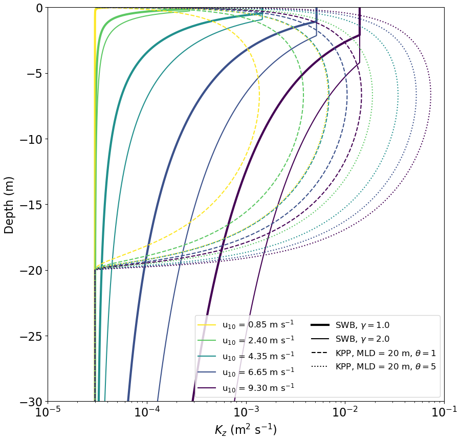
where $K_{\mathrm{B}}=\mathrm{3}\times {\mathrm{10}}^{-\mathrm{5}}$ m² s⁻¹ is the dianeutral diffusion below the MLD (Waterhouse et al., 2014). The diffusion is thus constant for $z>-\mathit{\gamma }{H}_{\mathrm{s}}$, below which $K_z\propto |z{|}^{-\mathrm{3}/\mathrm{2}}$, while the magnitude of K_z increases for higher wind speeds (Fig. 1). Poulain (2020) implies γ=1.0, while Kukulka et al. (2012) estimates γ≈1.5, and thus to test the model sensitivity we consider $\mathit{\gamma }\in [\mathrm{0.5},\mathrm{1.0},\mathrm{1.5},\mathrm{2.0}]$ (Fig. 1). As $z\to -\mathrm{\infty }$, $|z{|}^{-\mathrm{3}/\mathrm{2}}\to \mathrm{0}$, and therefore we include the bulk dianeutral diffusion K_B to account for vertical mixing at depths below the influence of surface wave-driven turbulence. As both Kukulka et al. (2012) and Poulain et al. (2019) considered turbulence generated by breaking surface waves, we refer to this diffusion approach as surface wave breaking (SWB) diffusion.

The second vertical diffusion coefficient profile is a local form of the KPP (Large et al., 1994; Boufadel et al., 2020), where K_z is given by

$$\begin{array}{}\text{(11)}& K_z=\left({\displaystyle \frac{\mathit{\kappa }{u}_{*\mathrm{w}}}{\mathit{\varphi }}}\mathit{\theta }\right)\left(\right|z|+z_{\mathrm{0}})\left(\mathrm{1}-{\displaystyle \frac{\left|z\right|}{\mathrm{MLD}}}\right)+K_{\mathrm{B}},\end{array}$$

where ϕ=0.9 is the “stability function” of the Monin–Obukhov boundary layer theory, θ is a Langmuir circulation (LC) enhancement factor and z₀ is the roughness scale of turbulence. As such, K_z​​​​​​​ rises from a small non-zero value at z=0 to a maxima at $z=\mathrm{1}/\mathrm{3}\mathrm{MLD}$, before dropping to K_z=K_B for z≤MLD (Fig. 1). In the original KPP formulation $K_z(z\le \mathrm{MLD})=\mathrm{0}$ since the theory only applies to the surface mixed layer, and thus we add the same bulk dianeutral diffusion term K_B as with the SWB profile (Eq. 10). Boufadel et al. (2020) examined a case where LC-driven turbulence was considered negligible, and thus θ=1.0. However, the presence of LC can increase turbulent mixing by a factor θ=3–4 (McWilliams and Sullivan, 2000) and has been shown to strongly affect the vertical concentration profiles of buoyant microplastic particles in LES experiments (Brunner et al., 2015; Kukulka and Brunner, 2015). Therefore, we examine $\mathit{\theta }\in [\mathrm{1.0},\mathrm{2.0},\mathrm{3.0},\mathrm{4.0},\mathrm{5.0}]$. The roughness scale z₀, which can represent the surface roughness due to surface waves, depends on the wind speed and the wave age (Zhao and Li, 2019), and following Kukulka et al. (2012) we consider a wave age ${\mathit{\beta }}_{*}=c_{\mathrm{p}}/u_{*\mathrm{a}}=\mathrm{35}$ that is equivalent to $\mathit{\beta }=c_{\mathrm{p}}/u_{\mathrm{10}}=\mathrm{1.21}$. According to Zhao and Li (2019), the roughness scale is given by

$$\begin{array}{}\text{(12)}& z_{\mathrm{0}}=\mathrm{3.5153}\times {\mathrm{10}}^{-\mathrm{5}}{\mathit{\beta }}^{-\mathrm{0.42}}{u}_{\mathrm{10}}^{\mathrm{2}}/g.\end{array}$$

For w₁₀=0.85–9.30 m s⁻¹, this means $z_{\mathrm{0}}=\mathrm{2.38}\times {\mathrm{10}}^{-\mathrm{6}}$–$\mathrm{2.86}\times {\mathrm{10}}^{-\mathrm{4}}$ m. To test the model sensitivity to z₀, we also consider an alternative scenario where $z_{\mathrm{0}}=\mathrm{0.1}\times H_{\mathrm{s}}=\mathrm{1.76}\times {\mathrm{10}}^{-\mathrm{3}}$–$\mathrm{2.10}\times {\mathrm{10}}^{-\mathrm{1}}$ m, following the same formulation $H_{\mathrm{s}}=\mathrm{0.96}{g}^{-\mathrm{1}}{\mathit{\beta }}_{*}^{\mathrm{3}/\mathrm{2}}{u}_{*\mathrm{a}}^{\mathrm{2}}$ as in Kukulka et al. (2012). This increases K_z for z≈0 but does not significantly affect the magnitude K_z at greater depths (Fig. B1). The original KPP theory does not explicitly account for surface wave breaking, which would lead to larger non-zero K_z at z=0. While we do not claim that setting $z_{\mathrm{0}}=\mathrm{0.1}\times H_{\mathrm{s}}$ means that our KPP profile accounts for surface wave breaking turbulent mixing, it allows us to investigate the influence higher near-surface mixing would have on the modeled vertical concentration profiles. The MLD is the maximum depth of the surface ocean boundary layer formed due to interaction with the atmosphere, and in KPP theory the MLD is defined as the depth where the bulk Richardson number Ri_B is first equal to a critical value Ri_crit. In the original formulation Ri_crit=0.3 (Large et al., 1994), but Ri_B can be difficult to compute in the field as this requires data for both vertical density and velocity shear profiles. In this study we prescribe MLD =20 m, as this falls within the range of the MLD for field data used to evaluate the model (see Sect. 2.3).

Figure 1 Vertical diffusion coefficient profiles for SWB and KPP diffusion under varying wind conditions. The KPP diffusion profile is calculated with z₀ according to Eq. (12).

2.3 Field data

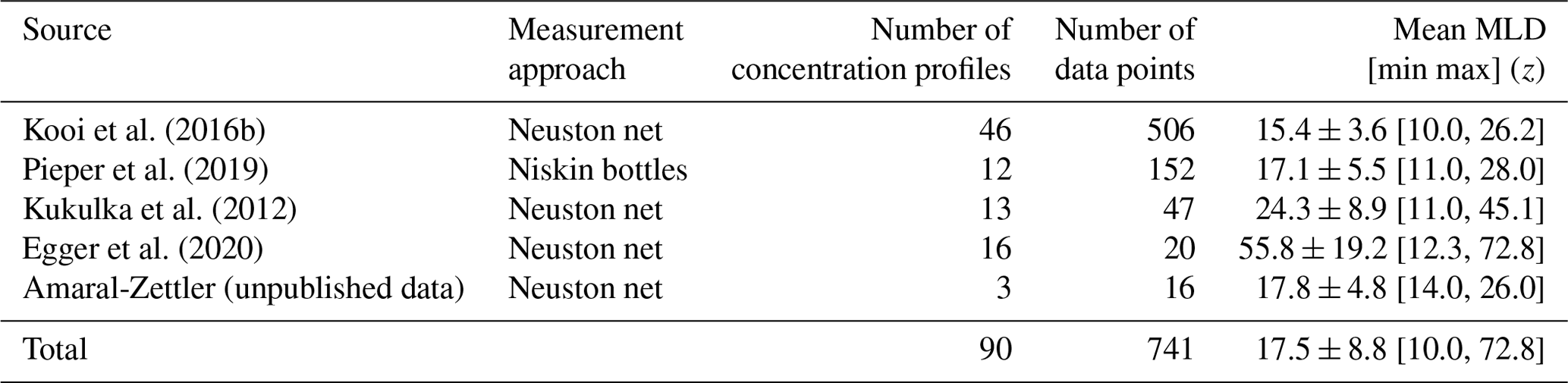
We compiled a dataset of vertical plastic concentration profiles collected within the surface mixing layer to validate the modeled concentration profiles (Table 1), with a total of 90 profiles with 741 data points. Only Kooi et al. (2016b) directly measured the rise velocity of a subsample of the collected microplastic particulates, and showed that these particles were positively buoyant. However, the presence of all the other sampled particulates near the open ocean surface indicates they are unlikely to be negatively buoyant. For all stations the wind speed was recorded and the MLD was determined from conductivity–temperature–depth (CTD) data based on a temperature threshold (de Boyer Montégut et al., 2004). The majority of the samples were collected in the North Atlantic (Kukulka et al., 2012; Kooi et al., 2016b; Pieper et al., 2019) and in regions with a relatively shallow MLD. Since wind-driven turbulent mixing is not expected to influence the concentration depth profile below the MLD, we do not consider any measurements collected below 73 m. Measurements were collected with surface wind speeds up to 10.7 m s⁻¹, with the majority of sampled concentrations being collected for u₁₀=3.4–7.9 m s⁻¹ (535 of the 741 data points).

Almost all of measurements were collected with neuston nets, either multi-level nets simultaneously sampling fixed depth intervals (Kooi et al., 2016b) or using multi-stage nets that consecutively sample fixed depths or depth ranges (Kukulka et al., 2012; Egger et al., 2020; Amaral-Zettler (unpublished data)). These nets have mesh sizes of 0.33 mm and will generally sample high- and medium-buoyancy (w_rise=0.03–0.003 m s⁻¹) particulates, which for non-biofouled polyethylene would have a diameter greater than the mesh size (2.2 and 0.4 mm). In contrast, low-buoyancy particulates (w_rise=0.0003 m s⁻¹) are typically not sampled in neuston nets (Kooi et al., 2016b), likely in part due to smaller particulate sizes. Pieper et al. (2019) filtered samples collected via Niskin bottles with a 0.8 µm filter and thus was able to filter out smaller particulates with lower rise velocities.

All measured microplastic concentrations are normalized by total amount of plastic measured within a vertical profile. In order to compare the average normalized field concentration with the modeled profiles, we bin the normalized field concentrations into 0.5 m depth bins and calculate the standard deviation for each depth bin. Comparison of the modeled concentration profiles with the binned normalized field measurements is done via the root-mean-square error (RMSE):

$$\begin{array}{}\text{(13)}& \mathrm{RMSE}=\sqrt{{\displaystyle \frac{\mathrm{1}}{n}}\sum _{i=\mathrm{0}}^n(C_{\mathrm{f},i}-C_{\mathrm{m},i})},\end{array}$$

where C_f,i and C_m,i are the binned normalized field measurement and modeled concentration within depth bin i. Model evaluation for the low-buoyancy particles is not possible with the available field measurements as low-buoyancy particles are typically too small to be sampled with neuston nets, and the Pieper et al. (2019) dataset alone is too small.

Kooi et al. (2016b)Pieper et al. (2019)Kukulka et al. (2012)Egger et al. (2020)

Table 1 Overview of the sources of field measurements of microplastic concentration profiles. The uncertainty in the mean MLD is the standard deviation.

3 Results

Starting with all particles at z=0 for t=0, M-0 models with both KPP and SWB diffusion lead to stable vertical concentration profiles (Fig. 2), where the equilibrium concentration profile is already established within 1–2 h (Fig. C1). For both diffusion profiles, there is progressively deeper mixing of particles with increasing wind speeds and decreasing buoyancy. While with both SWB and KPP diffusion low-buoyancy particles always get mixed below the surface, for medium- and high-buoyancy particles there exist minimum wind speeds below which all particles remain at the surface. These limits are similar for both diffusion types for medium-buoyancy particles (u₁₀≥2.40 m s⁻¹), but high-buoyancy particles only mix below the surface with SWB diffusion if u₁₀≥9.30 m s⁻¹. However, once mixing below the ocean surface occurs, KPP diffusion always leads to deeper mixing of particles than SWB diffusion due to higher subsurface K_z values.

The concentration profiles for medium- and low-buoyancy particles are largely unaffected by reducing Δt below 30 s (Fig. F1). However, for high-buoyancy particles with SWB diffusion the concentration profile more strongly depends on Δt due to the applied boundary condition. For Δt=30 s, the M-0 model shows all particles remain near the ocean surface, but shorter Δt values indicate that deeper mixing of particles already occurs for u₁₀=6.65 m s⁻¹. With KPP diffusion, all high-buoyancy particles remain at the surface even with Δt=1 s, as K_z at z=0 remains too low to overcome the high rise velocity.

Even though KPP diffusion with θ=1.0 and z₀ following (Zhao and Li, 2019) predicts deeper mixing of particles than with SWB diffusion (γ=1.0), both approaches underpredict the mixing of particles relative to field observations. For KPP diffusion, this can be corrected by accounting for LC-driven mixing, which leads to deeper mixing of particles for both medium- and low-buoyancy particles (Figs. 3 and D1). For medium-buoyancy particles this generally leads to better model agreement with lower RMSE values between the modeled and averaged field data concentration profiles (Fig. 5). However, for high-buoyancy particles LC-driven circulation is not enough as particles remain at the ocean surface for all wind conditions even for θ=5.0 (Fig. D2), as K_z for z≈0 is too low to overcome the inherent particle buoyancy. Only when LC-driven is combined with higher near-surface K_z values by setting $z_{\mathrm{0}}=\mathrm{0.1}\times H_{\mathrm{s}}$ do we see any below-surface mixing of high-buoyancy particles when θ>3.0 and u₁₀≥9.30 m s⁻¹. Increased near-surface K_z values have a lesser influence on the concentration profiles of medium- and low-density particles, as these particles were already being mixed below the surface even without larger z₀ values. For SWB diffusion we obtain deeper mixing of all particles by increasing γ>1.0 (Figs. 3, D1 and D2), which improves model performance relative to observations (Fig. 5). While increasing γ does not affect the peak magnitude of the near-surface K_z values, it increases the depth until which K_z is constant. This therefore results in stronger overall mixing (Fig. 4), which in turn leads to the deeper mixing of the particles.

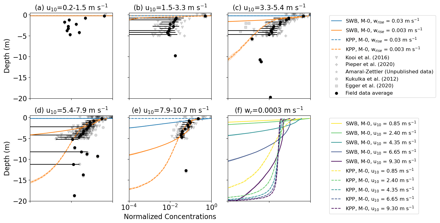
Figure 2 Vertical concentrations of buoyant particles for KPP and SWB diffusion using M-0 models. Panels (a)–(e) show the vertical concentration profiles for high- and medium-buoyancy particles with increasing wind speeds. The KPP profiles are calculated for θ=1.0 and z₀ according to Eq. (12). The grey markers indicate field measurements, with darker shades indicating more measurements, while the binned field measurement average and standard deviation are shown by the black markers. Panel (f) shows the vertical concentration profiles for low-buoyancy particles under increasing wind conditions. Shading around the profiles indicates the profile's standard deviation at each depth level.

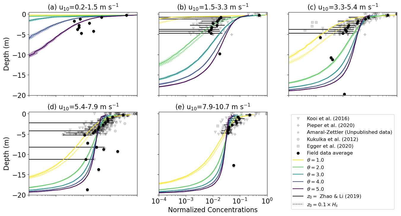
Figure 3 Vertical concentrations of buoyant particles for KPP diffusion using M-0 models for w_r=0.003 m s⁻¹. The KPP profiles are calculated for $\mathit{\theta }=[\mathrm{1.0},\mathrm{2.0},\mathrm{3.0},\mathrm{4.0},\mathrm{5.0}]$ and with either $z_{\mathrm{0}}=\mathrm{0.1}\times H_{\mathrm{s}}$ or according to Eq. (12). The grey markers indicate field measurements, with darker shades indicating more measurements, while the binned field measurement average and standard deviation are shown by the black markers. Shading around the profiles indicates the profile's standard deviation at each depth level.

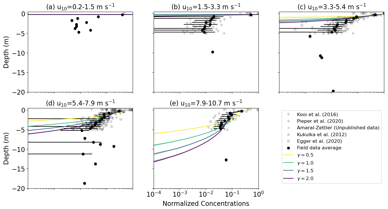
Figure 4 Vertical concentrations of buoyant particles for SWB diffusion under varying wind conditions with w_r=0.003 m s⁻¹. The SWB diffusion profile is calculated with $\mathit{\gamma }\in [\mathrm{0.5},\mathrm{1.0},\mathrm{1.5},\mathrm{2.0}]$. The grey markers indicate field measurements, with darker shades indicating more measurements, while the binned field measurement average and standard deviation are shown by the black markers. Shading around the profiles indicates the profile's standard deviation at each depth level.​​​​​​​

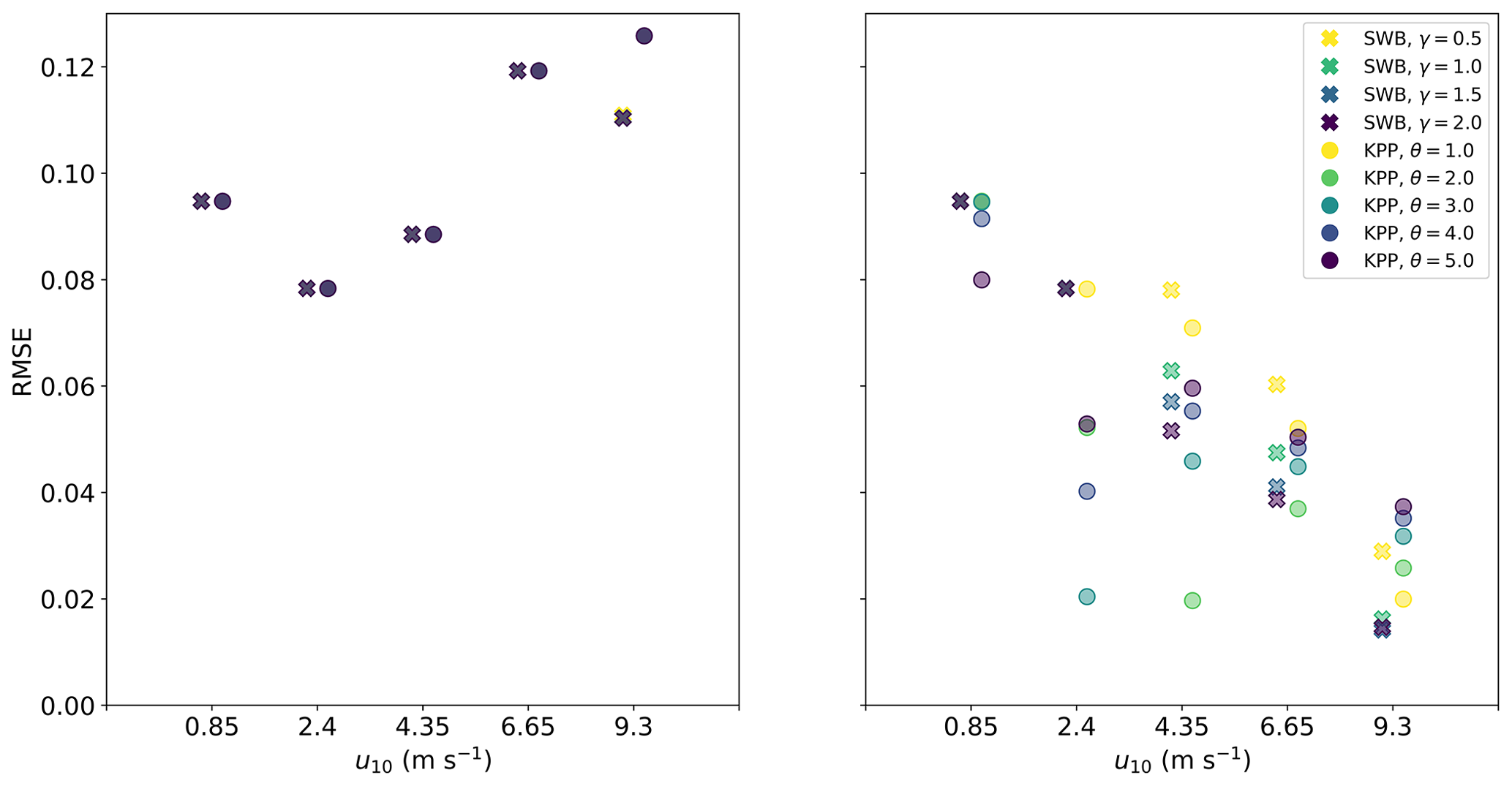
Figure 5 RMSE between field measurements and modeled concentration profiles for M-0 models with KPP and SWB diffusion under different wind conditions. All KPP diffusion simulations were with z₀ according to Eq. (12).

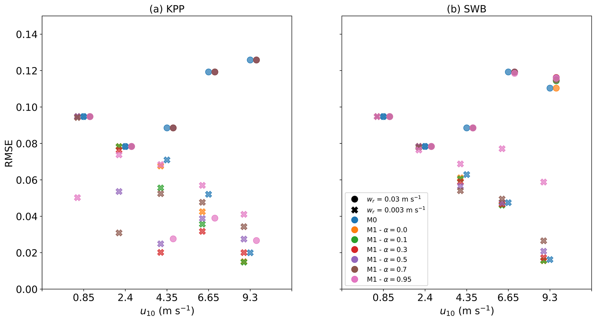
With both KPP and SWB diffusion, M-1 models show deeper mixing of particles as α→1 (Fig. 6). Relative to the field measurements, M-1 models can at best slightly improve model performance over M-0 models (Fig. 7). However, improved model performance is not shown across all particle sizes and wind conditions, and there is not a consistent α value leading to the smallest RMSE values.

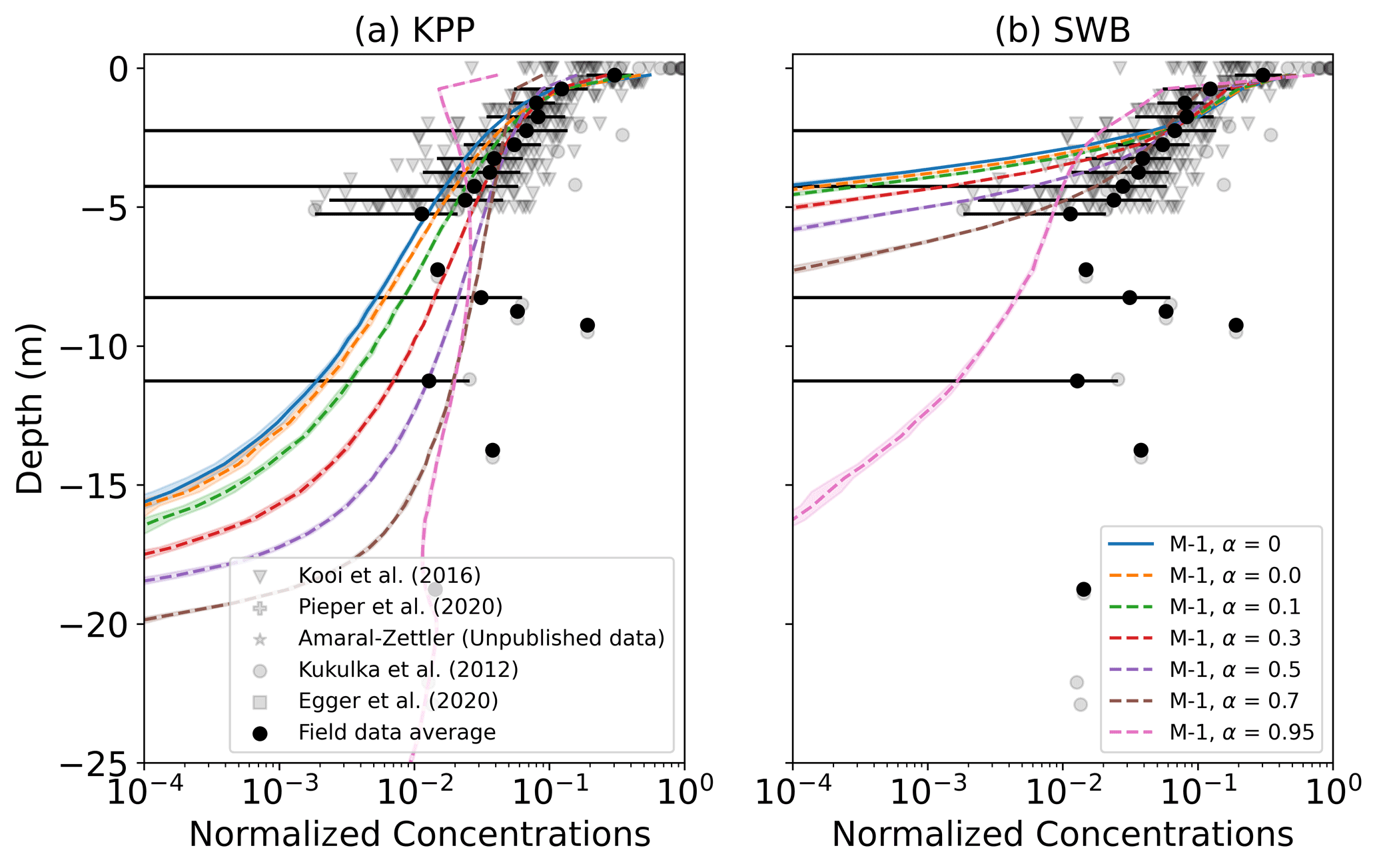
Figure 6 Vertical concentrations of buoyant particles for (a) KPP and (b) SWB diffusion using M-0 and M-1 models with varying values for α. The grey markers indicate field measurements, with darker shades indicating more measurements, while the binned field measurement average and standard deviation are shown by the black markers. Shading around the profiles indicates the profile's standard deviation at each depth level. The KPP profiles are for θ=1.0 and z₀ according to Eq. (12). All profiles are for u₁₀=6.65 m s⁻¹ and medium-buoyancy particles (w_rise=0.003 m s⁻¹).

Figure 7 RMSE between field measurements and modeled concentration profiles for M-0 and M-1 models with (a) KPP and (b) SWB diffusion under different wind conditions and with varying values of α. All KPP diffusion simulations were with θ=1.0 and z₀ according to Eq. 12.

4 Discussion

The parametrizations presented in this study are intended for use in 3D Lagrangian experiments using OGCM data and therefore should yield numerically stable results for the relatively large integration time steps used in large-scale Lagrangian vertical transport modeling (Lobelle et al., 2021). While there are more stable schemes available than the EM scheme used in this study (Gräwe et al., 2012), the EM scheme is computationally the cheapest and yields concentration profiles that match reasonably well with observations. Both M-0 and M-1 models show largely convergent concentration profiles for Δt=30 s, which would make both approaches feasible with regards to computational cost. However, we would currently recommend using a M-0 model. M-1 models have the additional tuning parameter α representing the autocorrelation of turbulent velocity fluctuations, which is poorly constrained in the literature. Using spatially invariant α values at best slightly improved model performance in comparison with M-0 models, and constraining α is not possible from these results. M-1 models may improve modeling of vertical diffusive transport, but more work is required to further constrain the value and vertical profile of α. Finally, numerous formulations of the M-1 drift term have been proposed (e.g., Mofakham and Ahmadi, 2020; Brickman and Smith, 2002) which can lead to large differences in the modeled profiles. In this study we used the non-normalized Langevin equation from Mofakham and Ahmadi (2020), but other formulations could be explored in future work.

While the concentration profiles of medium- and low-buoyancy particles are unaffected by decreasing the integration time step Δt<30 s, using higher Δt values underestimates the depth to which high-buoyancy particles are mixed when using SWB diffusion. This is because for high Δt values, the upward non-stochastic component of Eq. (6), which scales with Δt, dominates the stochastic component, which scales with $\sqrt{\mathrm{\Delta }t}$. With KPP diffusion the vertical profile for high-buoyancy particles appears unaffected by Δt, but this is because the near-surface K_z values are significantly lower than with SWB diffusion. One possibility to correct for this is to apply a different BC, such as a reflective BC. While the concentration profiles for medium- and low-buoyancy particles are not strongly affected by such a reflective BC (Fig. G1), the reflective BC does show deeper particle mixing with SWB diffusion. However, for Δt=30 s the depth of mixing is now overestimated compared to smaller Δt values (Fig. G2), as with Δt=30 s and w_r=0.03 m s⁻¹ the particle would be reflected up to 0.9 m below the ocean surface solely due to the model numerics. In addition, earlier studies have shown that reflecting BC can cause spurious increases in particle concentration near the boundary (Ross and Sharples, 2004; Nordam et al., 2019). Therefore, changing the BC to a reflective BC would not improve the concentration profiles of high-buoyancy particles. Depending on the model application and setup, the error in the concentration profile depth (𝒪(1) m for high-buoyancy particles) might be acceptable. Otherwise, the error can be reduced by using a smaller integration time step where that is computationally feasible.

Considering the KPP and SWB diffusion profiles, the results in this study are inconclusive with regards to which approach performs better relative to field observations. For high-buoyancy particles, SWB diffusion leads to slightly deeper particle mixing, while only if the KPP diffusion profile accounts for LC-driven turbulence and has higher near-surface K_z values can it similarly show below-surface mixing of high-buoyancy particles for u₁₀≥9.30 m s⁻¹. With medium- and low-buoyancy particles the KPP profile leads to much deeper mixing compared with SWB diffusion where γ=1.0 Poulain (2020), especially when accounting for LC-driven turbulence, and this appears to agree better with field observations. However, for SWB diffusion the value of γ is uncertain, as Poulain (2020) and Kukulka et al. (2012) define γ=1.0 and γ≈1.5, respectively. Higher γ values lead to approximately equal model performance relative to field observations as with KPP diffusion. However, the model evaluation is largely based on field measurements collected in the top 5 m of the water column, and it is below this depth that we see greater differences in the KPP and SWB vertical concentration profiles. In addition, the currently available data collected with neuston nets does not allow for model evaluation for the low-buoyancy particles in either scenario. As such, more field measurements (including smaller-sized particles) would be necessary to fully evaluate model performance for all particles sizes with the two diffusion profiles.

With regards to necessary data to calculate the diffusion profiles, the SWB approach has the benefit that it only requires surface wind stress data, while KPP diffusion additionally requires MLD data. In addition, while our results indicate that accounting for LC-driven turbulent mixing improves KPP diffusion model performance, determining which θ value to use is not trivial. McWilliams and Sullivan (2000) demonstrated that θ is inversely proportional to the Langmuir number (La), which is defined as $\mathrm{La}=\sqrt{u_{*\mathrm{w}}/U_{\mathrm{S}}}$ with U_S as the surface Stokes drift. The Langmuir number can conceivably be calculated using OGCM data, but the details of such an implementation will be left for future work with 3D Lagrangian models. However, KPP diffusion does have the advantage that it has been widely used and validated in various model setups (Boufadel et al., 2020; McWilliams and Sullivan, 2000; Large et al., 1994), while such extensive validation has not yet occurred for SWB diffusion. Finally, the influence of wind forcing on turbulence is generally assumed to be limited to the surface mixed layer (Chamecki et al., 2019), while with the SWB profile wind-generated turbulence can extend far below the MLD (Figs. 1 and E1), possibly overestimating turbulent mixing at such depths. KPP theory does limit wind-driven turbulent mixing to the surface mixed layer, while either a constant K_z value or other K_z profiles could be used for sub-MLD mixing, such as the K_z estimates for internal tide mixing as proposed by de Lavergne et al. (2020).

Ideally, KPP theory would be expanded to account for surface wave breaking, which could lead to higher near-surface K_z values as seen with MLD diffusion. While such a theoretical approach is beyond the scope of this paper, we show that artificially elevating near-surface K_z values by increasing the surface roughness z₀ has a smaller influence on the overall concentration profile than LC-driven mixing, as similarly shown by (Brunner et al., 2015). Therefore, although we recommend future work incorporating surface wave breaking into KPP theory, our current KPP diffusion approach representing LC-driving mixing through θ does already seem to capture the majority of turbulent mixing dynamics.

In all cases, the vertical concentration profiles stabilized to vertical equilibrium profiles, similar to what has been shown for buoyant particles in LES model studies (Liang et al., 2012; Yang et al., 2014; Brunner et al., 2015; Taylor, 2018). The modeled concentration profiles generally resembled the profiles from field measurements of microplastic concentrations under different wind conditions (Kooi et al., 2016b; Kukulka et al., 2012), but the averaged concentration profiles of the field measurements are quite noisy. This could be partly due to inhomogeneity in the particle buoyancy, as the collected microplastic particulates have varying sizes and rise velocities (Kooi et al., 2016b; Egger et al., 2020). Additionally, we sorted the field measurements based on wind conditions, but other underlying oceanographic conditions such as the MLD can still vary significantly even with similar wind speeds. Unfortunately, we lack additional data of the oceanographic conditions at the time of sampling, which currently prohibits more high-level comparisons of the field and model concentration profiles. Compared with the field data, the variance in the modeled concentration profiles is significantly smaller. This is in part also due to assuming constant environmental conditions over 12 h for the model simulations, while wind and other oceanographic conditions can change on much shorter timescales over the ocean surface. To further improve vertical transport model verification, more measurements would be required, covering a wider range of oceanographic conditions (such as for wind conditions higher than u₁₀=10.7 m s⁻¹) and with a high spatial sampling resolution also for depths $z<-\mathrm{5}$ m. Ideally these measurements would also sample small, neutrally buoyant particulates, but we acknowledge this is difficult with the sampling techniques commonly used today. At the same time, we would encourage conducting more ocean field measurements of near-surface vertical eddy diffusion coefficient and/or eddy viscosity profiles, as this will allow further validation of the K_z profiles predicted by the KPP and SWB theory with actual ocean near-surface mixing measurements.

The parameterizations have been validated for high and medium rise velocities, and at least for KPP diffusion with θ>1.0 the concentration profiles resemble those calculated from field observations. This provides confidence in the turbulence estimates from the KPP approach, and as these are independent of the type of particle that might be present, this would suggest the KPP approach can also be applied to neutral or negatively buoyant particles. However, as model verification was only possible for microplastic particulates with rise velocities between approximately 0.03 and 0.003 m s⁻¹, we would advise additional model verification for other particle types where the necessary field data are available. In the case of SWB diffusion, turbulent mixing seems underestimated when further from the ocean surface when γ=1.0, but increasing to γ=1.5–2.0 does correct for this. However, as SWB diffusion has not yet been as extensively tested and verified as KPP diffusion, we advise more caution and additional validation with field observations before applying this diffusion approach to other particle types.

5 Conclusions

We have developed a number of 1D surface mixing parametrizations designed to be readily applied in large-scale oceanic Lagrangian model experiments using OGCM data. Where possible, we would recommend using the turbulence fields from the OGCM to assure turbulent transport of the particles is consistent with that of other model tracers. However, if the turbulence fields are unavailable then particularly parametrizations with KPP diffusion with LC-driven mixing are shown to produce modeled vertical concentration profiles that match relatively well with field observations of microplastics. The parametrizations generally perform well for time steps of Δt=30 s, but for high-buoyancy particles users need to take care to use sufficiently short time steps, especially with SWB diffusion. Verification was only possible for positively buoyant particles larger than 0.33 mm (which generally have rise velocities ≤0.003 m s⁻¹), but the parametrizations should also be applicable to other particle types. The parametrizations can therefore be applied to investigate the influence of turbulent mixing on the vertical transport of (microplastic) particles within a 3D model setup, and ultimately gain a more complete understanding of the fate of such particles in the ocean.

Appendix A: $w_{\mathrm{r}}/w^{\prime }$ ratios for various turbulence scenarios

Table A1 Ratios $w_{\mathrm{r}}/w^{\prime }$ between the rise velocity w_r and the peak stochastic velocity perturbation w^′ for KPP and SWB diffusion. The peak w^′ is the maximum value of Eq. (3). The peak w^′ values for KPP diffusion are calculated for $\mathit{\theta }\in [\mathrm{1.0},\mathrm{3.0},\mathrm{5.0}]$ and for z₀ following Eq. (12). The peak w^′ values for SWB diffusion are independent of γ.

Appendix B: Influence of z₀ on diffusion profiles

Figure B1 Vertical diffusion coefficient profiles for KPP diffusion under varying wind conditions with θ=1.0. The KPP diffusion profile is calculated with either z₀ according to Eq. (12) or $z_{\mathrm{0}}=\mathrm{0.1}\times H_{\mathrm{s}}$.

Appendix C: Time evolution of concentration profiles

Figure C1 Vertical concentrations of buoyant particles for KPP diffusion at times t=0–12 h. The KPP diffusion profile is calculated with θ=1.0, u₁₀=6.65 m s⁻¹, and z₀ according to Eq. (12).

Appendix D: Influence of θ for KPP diffusion

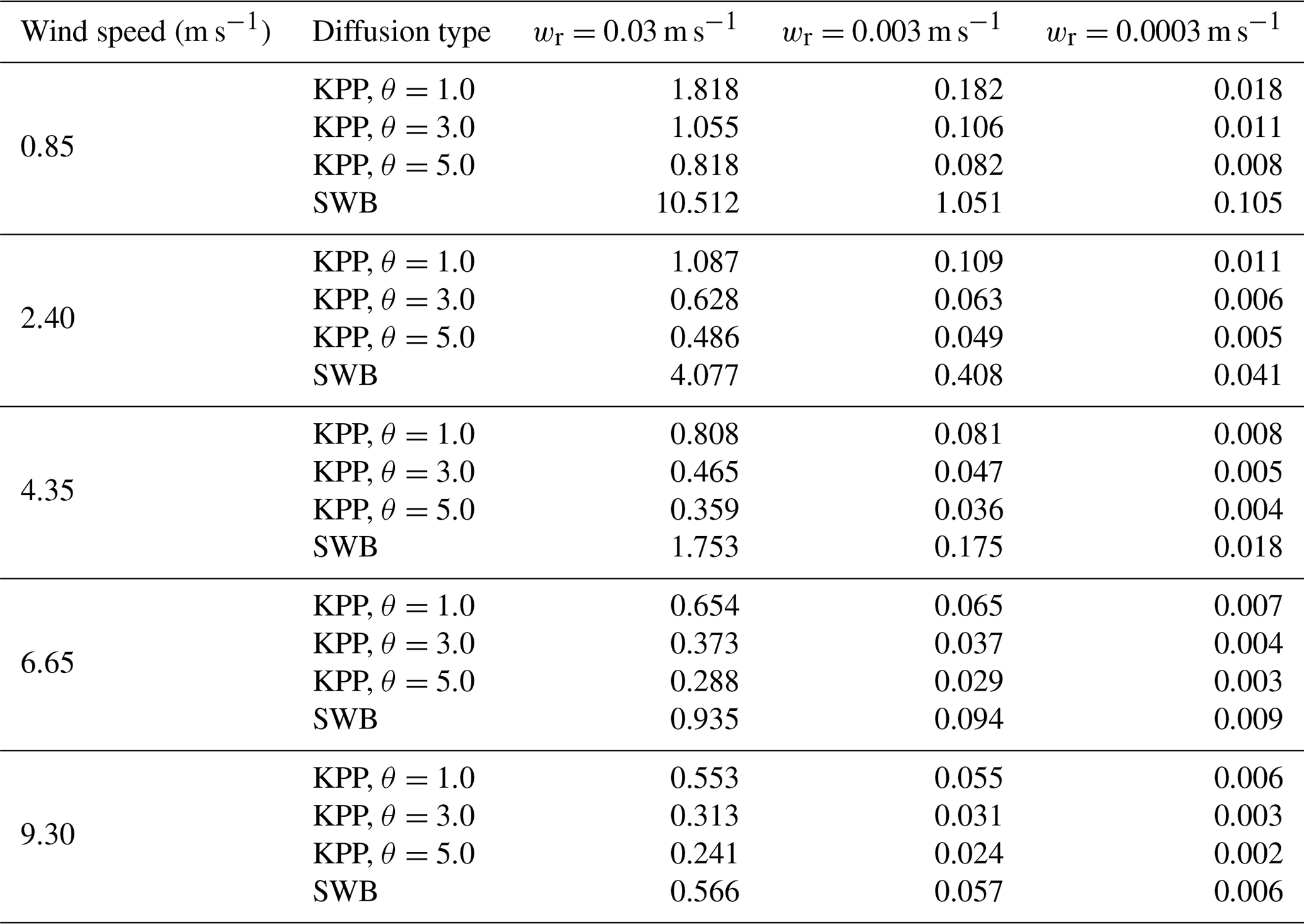
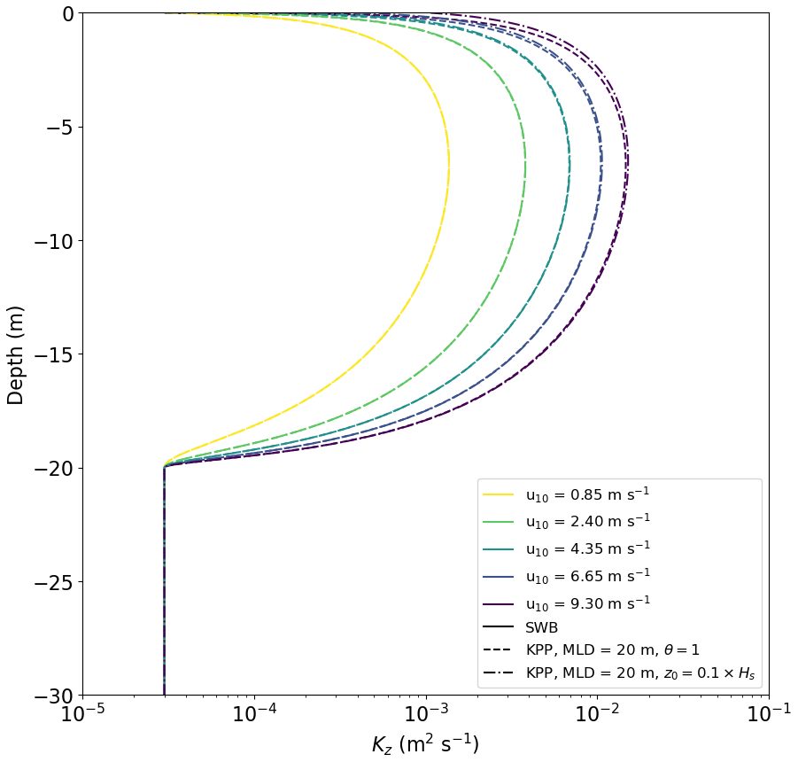
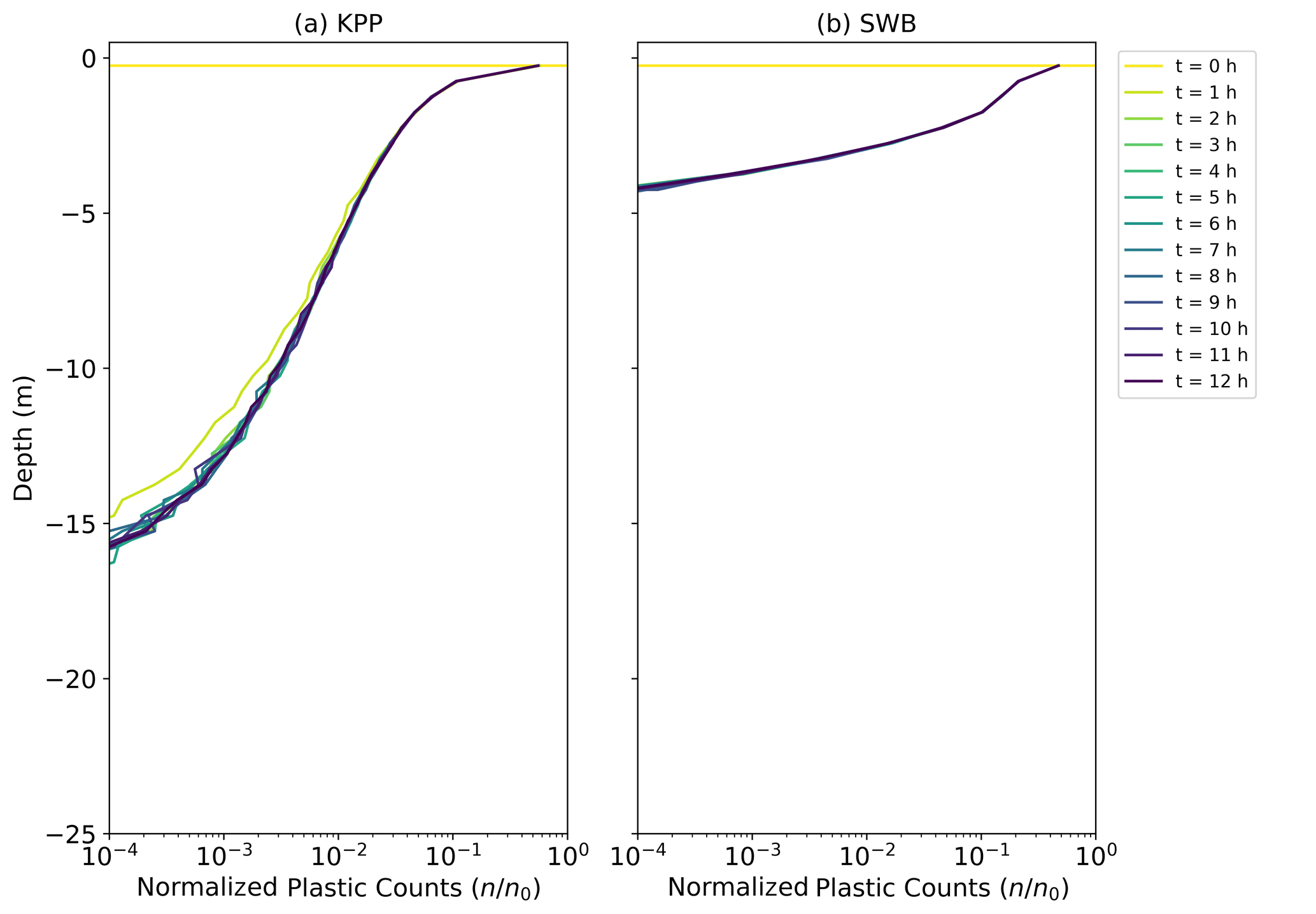
Figure D1 Vertical concentrations of buoyant particles for KPP diffusion under varying wind conditions with w_r=0.0003 m s⁻¹. The KPP diffusion profile is calculated with either z₀ according to Eq. (12) or $z_{\mathrm{0}}=\mathrm{0.1}\times H_{\mathrm{s}}$ and for $\mathit{\theta }\in [\mathrm{1.0},\mathrm{2.0},\mathrm{3.0},\mathrm{4.0},\mathrm{5.0}]$. The grey markers indicate field measurements, with darker shades indicating more measurements, while the binned field measurement average and standard deviation are shown by the black markers. Shading around the profiles indicates the profile's standard deviation at each depth level.

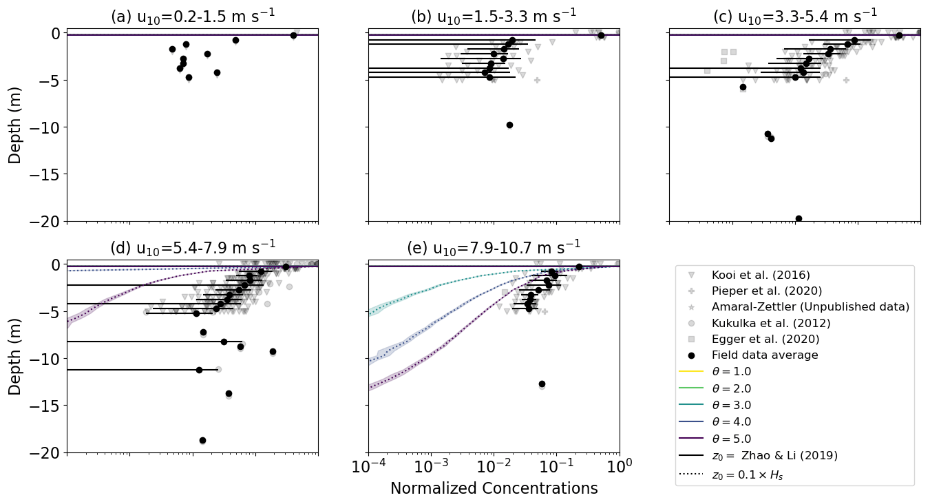
Figure D2 Vertical concentrations of buoyant particles for KPP diffusion under varying wind conditions with w_r=0.03 m s⁻¹. The KPP diffusion profile is calculated either with z₀ according to Eq. (12) or $z_{\mathrm{0}}=\mathrm{0.1}\times H_{\mathrm{s}}$ and for $\mathit{\theta }\in [\mathrm{1.0},\mathrm{2.0},\mathrm{3.0},\mathrm{4.0},\mathrm{5.0}]$. The grey markers indicate field measurements, with darker shades indicating more measurements, while the binned field measurement average and standard deviation are shown by the black markers. Shading around the profiles indicates the profile's standard deviation at each depth level.

Appendix E: Influence of γ for SWB diffusion

Figure E1 Vertical concentrations of buoyant particles for SWB diffusion under varying wind conditions with w_r=0.0003 m s⁻¹. The SWB diffusion profile is calculated with $\mathit{\gamma }\in [\mathrm{0.5},\mathrm{1.0},\mathrm{1.5},\mathrm{2.0}]$. The grey markers indicate field measurements, with darker shades indicating more measurements, while the binned field measurement average and standard deviation are shown by the black markers. Shading around the profiles indicates the profile's standard deviation at each depth level.

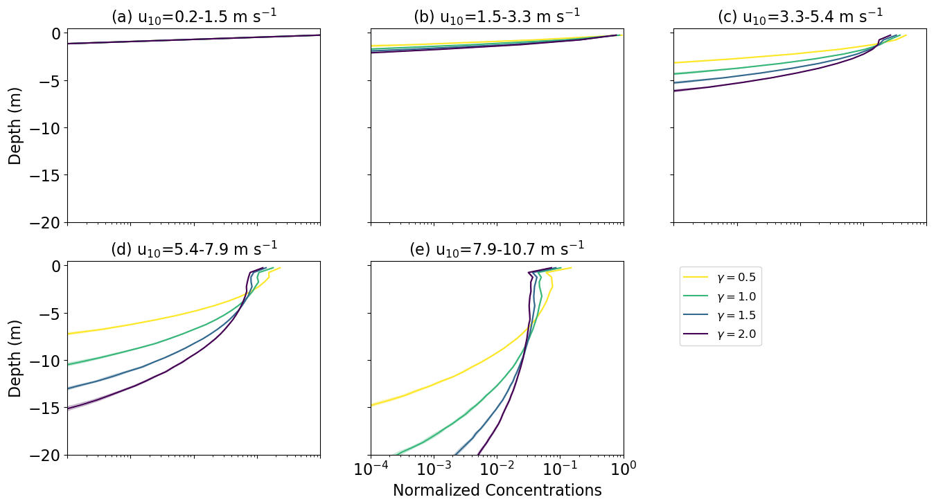
Figure E2 Vertical concentrations of buoyant particles for KPP diffusion under varying wind conditions with w_r=0.03 m s⁻¹. The SWB diffusion profile is calculated with $\mathit{\gamma }\in [\mathrm{0.5},\mathrm{1.0},\mathrm{1.5},\mathrm{2.0}]$. The grey markers indicate field measurements, with darker shades indicating more measurements, while the binned field measurement average and standard deviation are shown by the black markers. Shading around the profiles indicates the profile's standard deviation at each depth level.

Appendix F: Influence of Δt

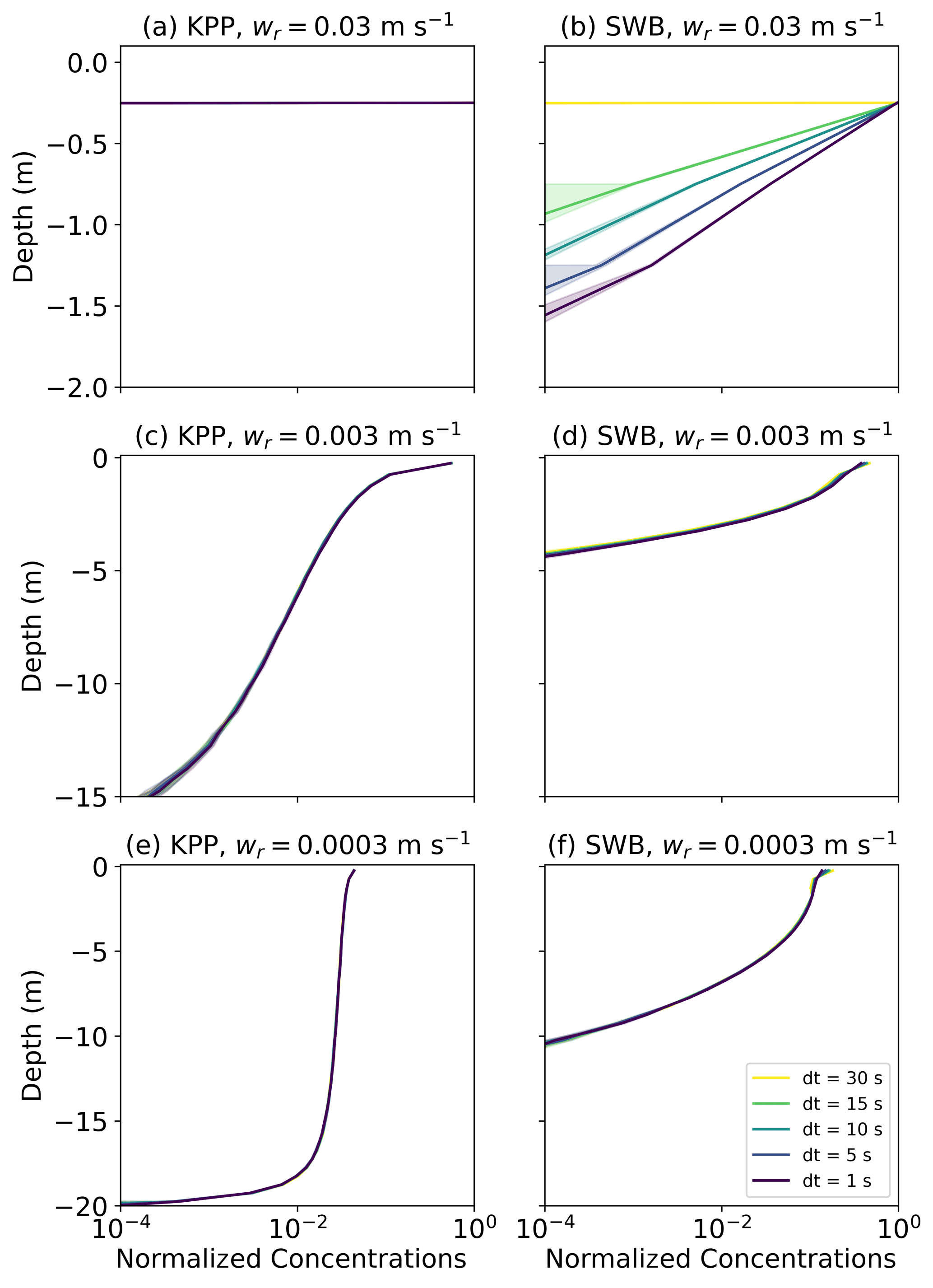
Figure F1 Vertical concentrations of buoyant particles for (a, c, e) KPP and (b, d, f) SWB diffusion using M-0 models with varying values for w_rise and $\mathrm{\Delta }t\in [\mathrm{30},\mathrm{15},\mathrm{10},\mathrm{5},\mathrm{1}]$ s. All profiles are for u₁₀=6.65 m s⁻¹. Shading around the profiles indicates the profile's standard deviation at each depth level. The KPP profiles are computed with θ=1.0 and z₀ according to Eq. (12), while the SWB profile is computed with γ=1.0.

Appendix G: Influence of boundary conditions

Figure G1 Vertical concentrations of buoyant particles for (a) KPP and (b) SWB diffusion using M-0 models for reflective and ceiling BCs. Shading around the profiles indicates the profile's standard deviation at each depth level. All profiles are for u₁₀=6.65 m s⁻¹. The KPP profiles are computed with θ=1.0 and z₀ according to Eq. (12), while the SWB profile is computed with γ=1.0.

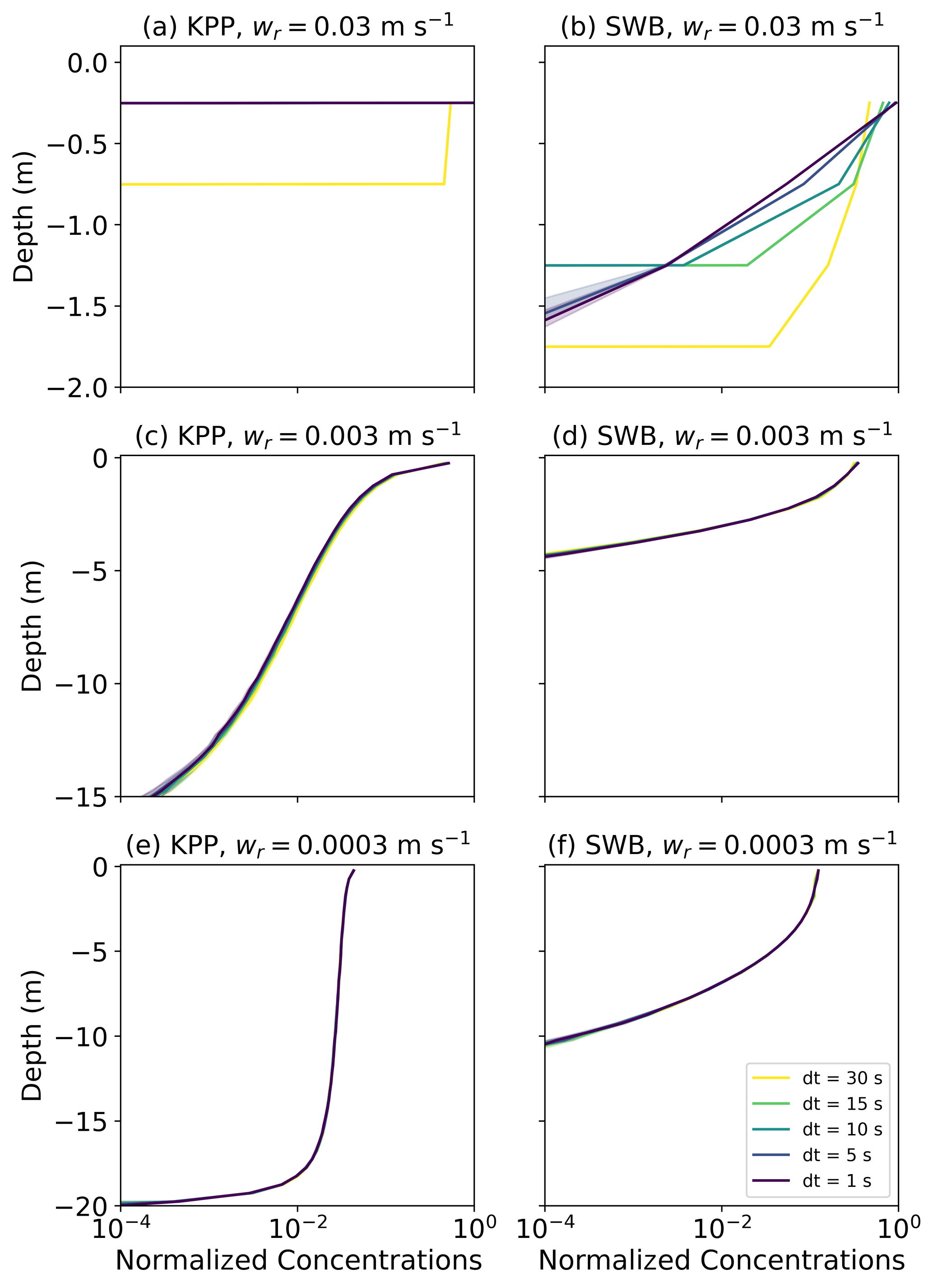
Figure G2 Vertical concentrations of buoyant particles for (a, c, e) KPP and (b, d, f) SWB diffusion using M-0 models with varying values for w_rise and $\mathrm{\Delta }t\in [\mathrm{30},\mathrm{15},\mathrm{10},\mathrm{5},\mathrm{1}]$ s with a reflective BC. All profiles are for u₁₀=6.65 m s⁻¹. Shading around the profiles indicates the profile's standard deviation at each depth level. The KPP profiles are computed with θ=1.0 and z₀ according to Eq. (12), while the SWB profile is computed with γ=1.0.