A three-dimensional variational data assimilation system for aerosol optical properties based on WRF-Chem v4.0: design, development, and application of assimilating Himawari-8 aerosol observations

This paper presents a three-dimensional variational (3DVAR) data assimilation (DA) system for aerosol optical properties, including aerosol optical thickness (AOT) retrievals and lidar-based aerosol profiles, developed for the Model for Simulating Aerosol Interactions and Chemistry (MOSAIC) within the Weather Research and Forecasting model coupled to Chemistry (WRF-Chem) model. For computational efficiency, 32 model variables in the MOSAIC_4bin scheme are lumped into 20 aerosol state variables that are representative of mass concentrations in the DA system. To directly assimilate aerosol optical properties, an observation operator based on the Mie scattering theory was employed, which was obtained by simplifying the optical module in WRF-Chem. The tangent linear (TL) and adjoint (AD) operators were then established and passed the TL/AD sensitivity test. The Himawari-8 derived AOT data were assimilated to validate the system and investigate the effects of assimilation on both AOT and PM_2.5 simulations. Two comparative experiments were performed with a cycle of 24 h from 23 to 29 November 2018, during which a heavy air pollution event occurred in northern China. The DA performances of the model simulation were evaluated against independent aerosol observations, including the Aerosol Robotic Network (AERONET) AOT and surface PM_2.5 measurements. The results show that Himawari-8 AOT assimilation can significantly improve model AOT analyses and forecasts. Generally, the control experiments without assimilation seriously underestimated AOTs compared with observed values and were therefore unable to describe real aerosol pollution. The analysis fields closer to observations improved AOT simulations, indicating that the system successfully assimilated AOT observations into the model. In terms of statistical metrics, assimilating Himawari-8 AOTs only limitedly improved PM_2.5 analyses in the inner simulation domain (D02); however, the positive effect can last for over 24 h. Assimilation effectively enlarged the underestimated PM_2.5 concentrations to be closer to the real distribution in northern China, which is of great value for studying heavy air pollution events.

1 Introduction

Atmospheric aerosols have considerable impacts on weather, climate, and human health (Menon et al., 2002; Qian et al., 2009; Gao et al., 2015). They are involved in many physical and chemical processes in the atmosphere, such as directly scattering and absorbing solar radiation, sources of cloud condensation nuclei, and air pollution (Pöschl, 2005; Gao et al., 2015; Q. Chen et al., 2019). Conventional observations such as surface mass concentration measurements play an important role in aerosol analysis and monitoring. For instance, the China National Environmental Monitoring Centre (CNEMC, http://www.cnemc.cn/en/, last access: 1 May 2021) has established a nationwide monitoring network consisting of more than 1500 stations since 2013 to provide near-time data of pollutants, including PM_2.5, PM₁₀, SO₂, NO₂, CO, and O₃. However, conventional observations alone are insufficient to describe three-dimensional aerosol distribution in detail because monitoring stations are mostly located in urban areas and aerosol profiles, which are important for studying aerosol transport, are scarce. Light extinction is an inherent property of aerosols, and different aerosol particles have different extinctions, and thus optical observations are utilized to study aerosols. Compared with conventional observations, Remote sensing optical properties can cover a much larger domain (Kaufman et al., 2002) and provide detailed aerosol profiles (Young and Vaughan, 2009), which are bound to extend the aerosol study. Furthermore, with the development of remote sensing technology, more aerosol optical properties have become available. For example, Moderate Resolution Imaging Spectroradiometer (MODIS) aerosol optical thickness (AOT) data have been widely used (Liu et al., 2011; Schwartz et al., 2012; Saide et al., 2013), Aerosol Robotic Network (AERONET; http://aeronet.gsfc.nasa.gov/, last access: 25 July 2021) (Holben et al., 1998) AOT observations have been used for aerosol analyses (Rubin et al., 2017; Dai et al., 2019), and AOT retrievals from the Japanese Himawari-8, a next-generation geostationary meteorological satellite, have been operationally used since 2015 (Sekiyama et al., 2016). Additionally, aerosol extinction or backscattering coefficients detected by ground-based lidar (Wang et al., 2014; Cheng et al., 2019) or space-borne lidar such as Cloud-Aerosol Lidar and Infrared Pathfinder Satellite Observation (CALIPSO) have also been employed to analyze aerosol profiles (Sekiyama et al., 2010).

Besides, numerical simulations conducted by atmospheric chemistry models or air quality models have increasingly played an essential role in aerosol analysis and prediction. Significant progress has been achieved in recent years; however, accurate aerosol modeling remains challenging given the large uncertainties associated with aerosol emissions, initial conditions, and complex interactions with meteorological processes. Solving these uncertainties is of great significance for improving aerosol modeling. Data assimilation (DA), a statistically optimal approach combining observations with numerical model outputs, can reduce uncertainties in the initial aerosol fields. Chemical DA, especially aerosol DA, has gradually developed to improve the prediction of air quality in recent years. In early studies of aerosol DA, the optimal interpolation (OI) technique was employed to assimilate the total mass concentrations of PM_2.5 or PM₁₀ using a control variable scheme (Tombette et al., 2009). The variational algorithm was also employed in some studies. Niu et al. (2008) used the three-dimensional variational (3DVAR) technique to assimilate dust aerosol observations based on one control variable and obtained a positive assimilation result. With an understanding of the aerosol chemical mechanism, as well as the improvement of computing performance, multi-variable aerosol DA studies were conducted, which mainly focused on the development of the 3DVAR technique and Coupled Chemistry Meteorology Model (CCMM). For example, the open-source Grid-point Statistical Interpolation (GSI) tool presented by National Centers for Environmental Prediction (NCEP) (Wu et al., 2002; Kleist et al., 2009) has been widely applied to aerosol DA (Pagowski et al., 2010; Liu et al., 2011; Jiang et al., 2013; Feng et al., 2018; Pang et al., 2018). The GSI tool was preliminarily developed for the Goddard Chemistry Aerosol Radiation and Transport (GOCART) aerosol scheme (Chin et al., 2000) using the 3DVAR algorithm. To overcome the systematic underestimation of the GOCART scheme in the assimilation context, researchers developed an aerosol DA system based on the Model for Simulating Aerosol Interactions and Chemistry (MOSAIC) aerosol scheme (Li et al., 2013; Zang et al., 2016; Wang et al., 2020; Liang et al., 2020). For instance, Li et al. (2013) lumped eight aerosol species within MOSAIC into five control variables and then constructed a 3DVAR DA system to assimilate PM_2.5 mass concentrations, and the results showed that DA has a beneficial effect on both the initial field and PM_2.5 forecasts within a 24 h period. Although the four-dimensional variational (4DVAR) technique has been extensively used in operations (Gauthier at al., 2007; Benedetti et al., 2019) and has also been employed to assimilate atmospheric chemical compositions such as O₃, SO₂, and CO based on the simple offline chemical transport model (CTM) (Eibern and Schmidt, 1999; Elbern and Schmidt, 2001), it is greatly challenging to develop a 4DVAR DA system coupled with the sophisticated aerosol model such as MOSAIC because of the high computational cost and complex adjoint model. Consequently, the 3DVAR algorithm is still commonly used for aerosol DA.

As mentioned above, optical properties have great potential for studying aerosols, and thus it is natural to incorporate them into models via assimilation. The key issue of directly assimilating aerosol optical properties is the establishment of an observation operator and its adjoint for variational methods. Liu et al. (2011) added the forward AOT operator and its adjoint module within the Community Radiative Transfer Model (CRTM) (Han et al., 2006) to the GSI for the first time and successfully assimilated MODIS AOTs. This extended assimilation tool was then employed to assimilate various AOT retrievals from different platforms (Schwartz et al., 2012; Saide et al., 2014; Tang et al., 2017; Pang et al., 2018; Ha et al., 2020) and achieved encouraging results. Similar to AOT, assimilating lidar aerosol profiles also involves the complex forward operator and its adjoint (Cheng et al., 2019; Wang et al., 2014). In order to simplify the observation operator, an approximate approach was utilized to directly assimilate aerosol profiles. For example, Liang et al. (2020) employed the Interagency Monitoring of Protected Visual Environments (IMPROVE) equation, which is the linear link between the extinction coefficient and aerosol chemical species mass, as the forward operator to construct a 3DVAR DA system and then assimilated ground-based lidar aerosol profiles and PM_2.5 mass concentrations simultaneously. In addition, some researchers have used sequential approaches, such as the ensemble Kalman filter, to advance aerosol DA (Schutgens et al., 2010; Yumimoto et al., 2016; Sekiyama et al., 2016; Dai et al., 2019). Nevertheless, the ensemble-based aerosol forecasts are very expensive due to the heavy computational load, especially for online meteorology–chemistry modeling, and it is thus difficult to widely implement them in the operational air quality DA systems (Pang and Wang, 2021).

Following Li et al. (2013) and You (2017), this study further extends the assimilation of aerosol optical properties. Using an observation operator based on the Mie scattering theory, a comprehensive 3DVAR DA system aiming for aerosol optical properties, including AOT retrievals and aerosol profiles, is developed for the MOSAIC aerosol scheme within the Weather Research and Forecasting model coupled to Chemistry (WRF-Chem) model for the first time. The remainder of this paper is organized as follows. Section 2 presents the aerosol DA system in detail. The data and experimental methods used in this study are described in Sect. 3. The background error statistics necessary for the assimilation experiment are analyzed in Sect. 4. The results are summarized in Sect. 5, discussing the assimilation effects. Finally, a summary is presented in Sect. 6, along with discussions on the limitations of this study and suggestions for future research.

2 Aerosol data assimilation design

2.1 Model description

WRF-Chem is an advanced online coupled meteorology–aerosol model (Grell et al., 2005) that can simultaneously simulate meteorological fields and atmospheric chemical compositions including aerosols. It has been widely used in air quality forecasting and aerosol-related studies (Chen et al., 2016). Aerosol processes are treated by modules or schemes in WRF-Chem, such as GOCART (Chin et al., 2000), MOSAIC (Zaveri et al., 2008), and Modal Aerosol Dynamics Model for Europe (MADE) (Ackermann et al., 1998). There is no size information except total mass for sulfate, black carbon (BC), and organic carbon (OC), while there is only size information for dust and sea salt in GOCART, in addition to no description of second organic aerosol (SOA), resulting in its numerical efficiency. Due to more detailed descriptions of dust, GOCART has been applied more extensively in dust aerosol research. MADE is a modal aerosol scheme that describes more aerosol species than GOCART, including sulfate, ammonium salt, black carbon, organic carbon, sea salt, nitrate, dust, and SOA. Moreover, it employs three log-normal modes, that is, Aitken, accumulation, and coarse, to describe aerosol size distributions in detail. Although such a scheme is ideal for aerosols, it consumes more computational resources; therefore, its applications are limited. As a newly developed scheme, MOSAIC is a sectional aerosol scheme that incorporates tradeoffs between detailed descriptions of aerosol chemical species, size distributions, and computational cost. Previous studies have shown that this scheme has a good ability to simulate the compound aerosol pollution process in China (Gao et al., 2015; D. Chen et al., 2016, 2019). The MOSAIC scheme divides atmospheric aerosols into eight species, including BC, OC, nitrate (NO${}_{\mathrm{3}}^{-}$), sulfate (SO${}_{\mathrm{4}}^{\mathrm{2}-}$), chloride (Cl⁻), sodium (NA⁺), ammonium salt (NH${}_{\mathrm{4}}^{+}$), and other unclassified inorganic mass (OIN). At the same time, four or eight discrete size sections or bins are employed to represent the size distribution of each species. In this study, we selected four bins for computational efficiency. The first, second, third, and fourth size sections are set to be 0.0390625–0.15625, 0.15625–0.625, 0.625–2.5, and 2.5–10.0 µm, respectively. The sum of the eight species in the first three sections corresponds to PM_2.5, whereas the sum of all the sections corresponds to PM₁₀. This approach ensures that aerosols are represented efficiently and accurately. Thus, it can be concluded that the MOSAIC aerosol mechanism of multiple species in multi-particle size sections has an advantage in anthropogenic aerosol studies over other schemes. Therefore, we conducted aerosol analyses and forecasts using MOSAIC, and a DA system was developed for the MOSAIC scheme.

The WRF-Chem version 4.0 was used to perform assimilation simulation experiments. Both physical and chemical parameterization schemes are indispensable for numerical simulations. The main parameterization schemes used in this study include the WRF single-moment six-class microphysics scheme (WSM6, Hong and Lim, 2006), the Rapid Radiative Transfer Model for General Circulation Model (RRTMG) longwave and shortwave radiation scheme (Iacono et al., 2008), the Noah land surface scheme (Chen and Dudhia, 2001), the Yonsei University (YSU) atmospheric boundary layer scheme (Hong and Lim, 2006), the Grell–Freitas convective parameterization scheme, the Fast-J photolysis scheme (Ruggaber et al., 1994), the Regional Acid Deposition Model, Version 2 (RADM2, Stockwell et al., 1990), the Modal Aerosol Dynamics Model for Europe (MADE, Ackermann et al., 1998) and Second Organic Aerosol Model (SORGAM, Schell et al., 2001) anthropogenic emissions, and the MOSAIC_4bin scheme described above.

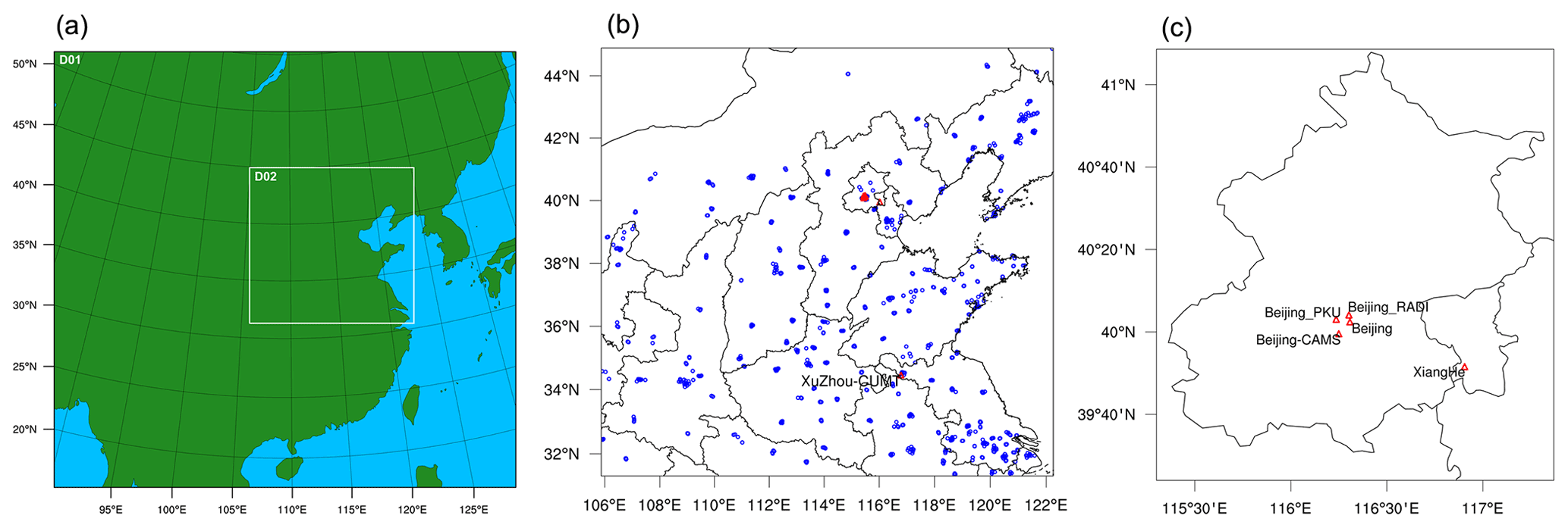
Figure 1 Configuration of the two-level nested domain used in this study (a), the monitoring stations in Domain 2 (D02) (b), and a zoomed-in map for AERONET sites in Beijing area (c), including Beijing, Beijing-CAMS, Beijing_PKU, Beijing_RADI, and XiangHe. There are a total of 683 surface ambient air quality monitoring stations represented by little blue circles, which are mainly located in urban areas, as well as six AERONET sites represented by red triangles in D02. All the maps are plotted with NCAR Command Language Version 6.6.2.

The configuration of the two-level nested simulation domain is shown in Fig. 1a, including most of East Asia in Domain 1 (hereafter denoted as D01) with a horizontal grid spacing of 27 km, and the entirety of northern China as well as parts of East and Central China in Domain 2 (hereafter denoted as D02) with a horizontal resolution of 9 km, one-third that of D01. To ensure a detailed simulation of aerosol vertical distributions, 40 vertical layers were modeled in the simulation, and it is worth mentioning that the vertical axis is on hybrid sigma-pressure levels with a resolution decreasing with height. The lowest layer is at the surface, whereas the top reaches 50 hPa.

2.2 Basic formulation

The 3DVAR algorithm has been extensively used for aerosol analysis and forecasts, such as the GSI tool, because of its high computational efficiency and the advantages of handling unconventional observations. Thus, it was employed to construct a DA system aiming for aerosol optical properties in this study. The 3DVAR algorithm can produce an aerosol analysis field with minimum analysis error covariance after a correction to the background field through the introduction of various observation information. For this purpose, an incremental approach was adopted, similar to the operational use in meteorology (Courtier et al., 1998). In its incremental formulation, 3DVAR attempts to minimize the cost function J.

$$\begin{array}{}\text{(1)}& J\left(\mathit{\delta }\mathit{x}\right)={\displaystyle \frac{\mathrm{1}}{\mathrm{2}}}\mathit{\delta }{\mathit{x}}^{\mathrm{T}}{\mathbf{B}}^{-\mathrm{1}}\mathit{\delta }\mathit{x}+{\displaystyle \frac{\mathrm{1}}{\mathrm{2}}}{\left(\mathbf{H}\mathit{\delta }\mathit{x}-\mathit{d}\right)}^{\mathrm{T}}{\mathbf{R}}^{-\mathrm{1}}\left(\mathbf{H}\mathit{\delta }\mathit{x}-\mathit{d}\right),\end{array}$$

where δx is the increment, corresponding to an aerosol state vector that defines the state variables of three-dimensional grid, also known as control variables in the DA process. At the minimum, the resulting analysis increment δx^a is added to the background x^b to provide the analysis x^a. B is the background error covariance matrix, and d is the innovation vector, which is expressed as follows:

$$\begin{array}{}\text{(2)}& \mathit{d}=\mathit{y}-H\left[{\mathit{x}}^{\mathrm{b}}\right],\end{array}$$

where y is the observation vector. H is a suitable linear approximation of the observation operator H in the vicinity of x^b, known as the tangent linear (TL) operator, and its transpose is the adjoint (AD) operator (see below). R is the observation error covariance matrix. Section 5 describes the calculation of B. In most cases, observations are independently conducted, and thus R is assumed to be a diagonal matrix without correlations among different observation errors considered. In general, observation errors associated with AOT retrievals are determined by measurement and representation errors (Elbern and Schmidt, 2001; Schwartz et al., 2012; Jiang et al., 2013). According to Yumimoto et al. (2016), the observation error of Himawari-8 AOT retrievals is set to 0.06 in this study. However, further studies into observation errors of aerosol optical properties are necessary.

The search for a minimum solution to the cost function usually involves a numerical iterative process using a descent algorithm. However, it is difficult to solve using Eq. (1) because it includes the inverse of B. We used the methods of Li et al. (2013) to deal with the inversion of B. First, B can be represented as the product of submatrices (Bannister, 2008), B=DCD^T, where D is the background error standard deviation (SD) matrix and C is the background error correlation matrix. Second, a Cholesky factorization is applied to C because it is a symmetric and positive definite matrix. The Cholesky factorization is as follows:

$$\begin{array}{}\text{(3)}& \mathbf{C}={\mathbf{C}}^{\mathrm{1}/\mathrm{2}}{\left({\mathbf{C}}^{\mathrm{1}/\mathrm{2}}\right)}^{\mathrm{T}},\end{array}$$

where the matrix ${\mathbf{C}}^{\mathrm{1}/\mathrm{2}}$ is a lower triangular matrix. Using this Cholesky factorization, we can transform the control variables δx to δz through

$$\begin{array}{}\text{(4)}& \mathit{\delta }\mathit{x}={\mathbf{DC}}^{\mathrm{1}/\mathrm{2}}\mathit{\delta }\mathit{z}.\end{array}$$

Finally, substituting Eq. (4) into Eq. (1), we obtain the desired form of Eq. (1) as follows:

$$\begin{array}{}\text{(5)}& \begin{array}{rl}J\left(\mathit{\delta }\mathit{z}\right)& ={\displaystyle \frac{\mathrm{1}}{\mathrm{2}}}\mathit{\delta }{\mathit{z}}^{\mathrm{T}}\mathit{\delta }\mathit{z}+{\displaystyle \frac{\mathrm{1}}{\mathrm{2}}}{\left({\mathbf{HDC}}^{\mathrm{1}/\mathrm{2}}\mathit{\delta }\mathit{z}-\mathit{d}\right)}^{\mathrm{T}}\\ & \times {\mathbf{R}}^{-\mathrm{1}}\left({\mathbf{HDC}}^{\mathrm{1}/\mathrm{2}}\mathit{\delta }\mathit{z}-\mathit{d}\right).\end{array}\end{array}$$

The transformed cost function is generally better conditioned, and thus this transformation expedites convergence when it is iteratively minimized. Along with the cost function J(δz) computed at each iterative step, the derivative of J(δz) with respect to δz is computed as follows:

$$\begin{array}{}\text{(6)}& \mathrm{\nabla }J\left(\mathit{\delta }\mathit{z}\right)=\mathit{\delta }\mathit{z}+{\left({\mathbf{DC}}^{\mathrm{1}/\mathrm{2}}\right)}^{\mathrm{T}}{\mathbf{H}}^{\mathrm{T}}{\mathbf{R}}^{-\mathrm{1}}\left({\mathbf{HDC}}^{\mathrm{1}/\mathrm{2}}\mathit{\delta }\mathit{z}-\mathit{d}\right).\end{array}$$

The iteration starts with δz=0 and does not finish until the convergence condition is met or it reaches the maximum number of iterations. The descent algorithm used is the limited memory BFGS method (L-BFGS) (Liu and Nocedal, 1989). Finally, a return from the resulting δz at the minimum to δx^a is obtained through Eq. (4).

2.3 Control variables

As discussed above, the basic framework of Li et al. (2013) was employed to develop a DA system. To assimilate aerosol optical properties, a set of control variables different from those of Li et al. (2013) was designed, which are key elements in the DA system. The control variables vary with the aerosol scheme. Because the background field x^b was simulated with the MOSAIC_4bin scheme within WRF-Chem described in Sect. 2.1, the control variables should be designed according to the MOSAIC aerosol scheme. A total of 32 model variables represent the mass concentrations of eight species in the four bins within MOSAIC. If these model variables are directly taken as control variables, the resulting increments directly correspond to the model variables and can be added to the background to produce an analysis without intermediate conversions. However, such a number of control variables, much more than those in meteorological DA, will cause a heavy burden on computational and memory resources and even lead to computational non-convergence when the cost function is iteratively minimized. Therefore, a reduction in the model variables is essential for a stable and efficient assimilation system, meaning that the model variables should be lumped into fewer control variables in the DA process. The control variables generally depend on the available observations to be assimilated. For example, when assimilating routine aerosol measurements, such as the total mass concentrations of PM_2.5 and PM₁₀, the lumped control variables represent the total mass concentrations of different aerosol species without the size information included. For instance, the four model variables for sulfate. so4_a01, so4_a02, so4_a03, and so4_a04, were reduced to two control variables: one was the sum of so4_a01, so4_a02, and so4_a03, and the other was so4_a04 itself (Wang et al., 2020). However, for aerosol optical properties, the size information must be reserved within the control variables because aerosol particles with different size distributions have significantly different light extinctions. Nevertheless, some species have similar optical characteristics, including density and complex refractive indices, such as sulfate (SO${}_{\mathrm{4}}^{\mathrm{2}-}$), nitrate (NO${}_{\mathrm{3}}^{-}$), and ammonium salt (NH${}_{\mathrm{4}}^{+}$) (Barnard et al., 2010). Thus, we lumped these species so that the species treated by the assimilation system were reduced to black carbon; organic carbon; the summation of sulfate, nitrate, and ammonium salt; the summation of chlorides and sodium salts, which are quite rare inland; and other unclassified inorganics, and these five species were denoted by EC, OC, SSN, CN, and OIN, respectively (You, 2017); the size information of these species was retained using the same four bins as in Sect. 2.1. Consequently, there are a total of 20 control variables, named after EC1, EC2, EC3, EC4, OC1, OC2, OC3, OC4, SSN1, SSN2, SSN3, SSN4, CN1, CN2, CN3, CN4, OIN1, OIN2, OIN3, and OIN4, where the numbers 1, 2, 3, and 4 represent the four size sections, respectively. These control variables can easily be obtained from the model variables and represent the mass concentrations of the five aerosol species within the four bins. It should be noted that the direct result of assimilating is to generate the increments of 20 control variables above here, and the increments of lumped variables should be distributed into individual model variable within MOSAIC. For instance, the increment of SSN1 is equal to the summation of that of the model variables so4_a01, no3_a01, and nh4_a01. For simplicity, the distribution ratio was determined using the mass concentration background error SD for each model variable. When the increment of each model variable is obtained, directly adding that to its background value will produce an aerosol analysis.

2.4 Observation operator and its adjoint

The observation operator transforms the control variables into an equivalent of each observed quantity at the observation locations. Thus, a comparison between the simulations and observations can be performed, upon which the resulting increments depend. A nonlinear operator based on the Mie scattering theory was employed to directly assimilate aerosol optical properties. Specifically, the 20 control variables described in Sect. 2.3 are used to compute optical parameters, such as aerosol extinction coefficient at every model grid point, and then both horizontal and vertical interpolations of the simulations from the model grid to observation locations are performed. This approach ensures that the simulated and observed quantities are comparable to each other. The process of the forward observation operator is to compute aerosol optical properties through the control variables, as shown in Fig. 2, based on the work of Wang et al. (2014) and Barnard et al. (2010).

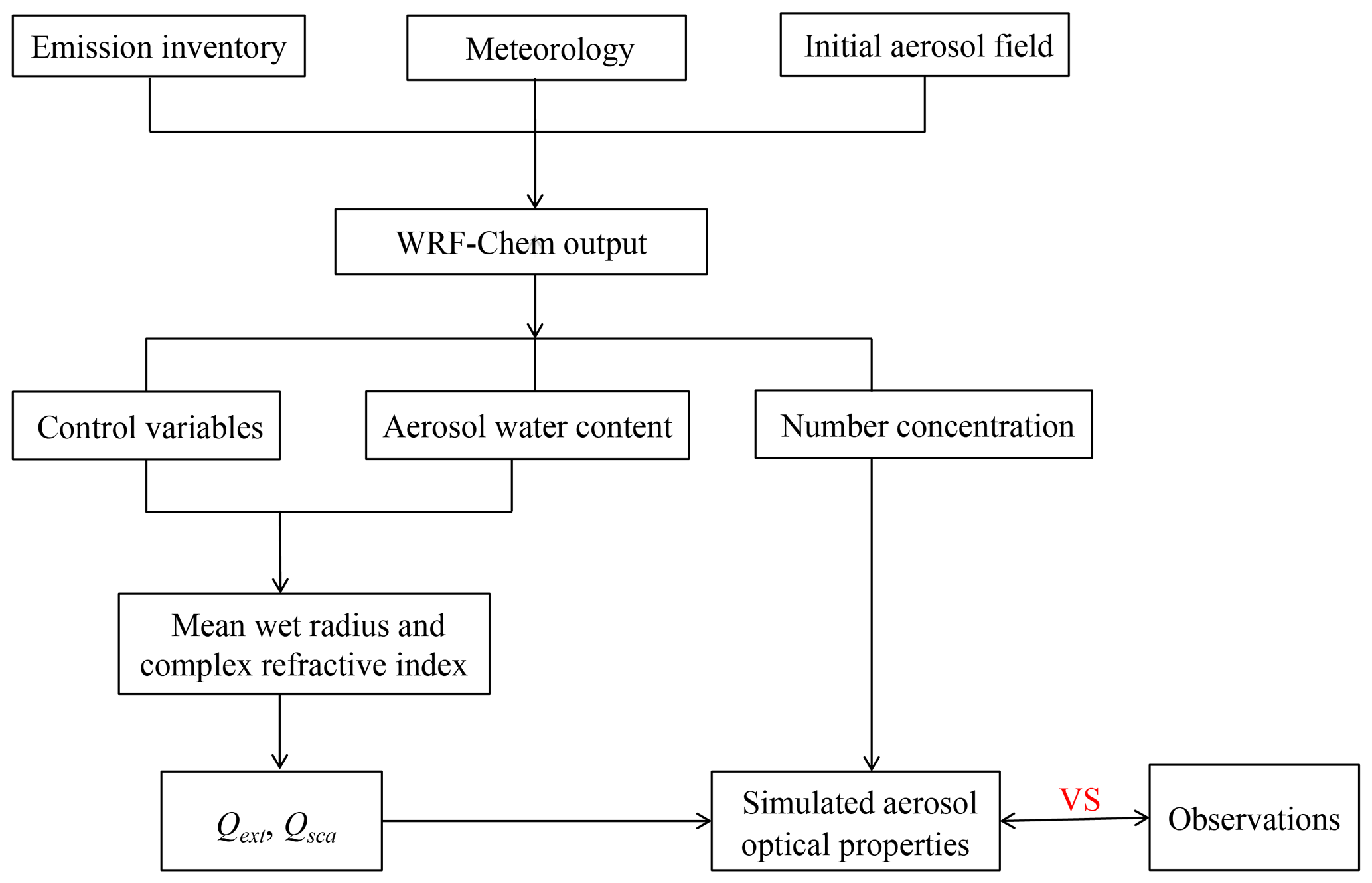
Figure 2 Diagram describing the forward observation operator used to transform aerosol mass concentrations to optical parameters. Q_ext and Q_sca are extinction and scattering efficiencies, respectively, which are functions of the size parameter and complex refractive index.

Although computing aerosol optical properties with WRF-Chem outputs involves many aerosol variables, as shown in Fig. 2, for simplicity, only mass concentrations measured routinely were set as the control variables. The forward operator is composed of several steps as follows. First, it is assumed that aerosol chemical species are internally mixed along with water in each bin. Given the densities of five assimilated species and water, individual volume is easily obtained so that the mean wet radius r_i assigned to each bin can be computed by dividing the total volume by the number concentration N_i, assuming that the particles are spherical, where the subscript i denotes the size bin. The particle size parameter is of significant importance to optical properties and is determined by $x=\mathrm{2}\mathit{\pi }{r}_i/\mathit{\lambda }$, where λ is the incident wavelength. Each species is associated with a complex index of refraction, and while these indices depend on λ, they vary little in the shortwave range where aerosols are remotely measured. The indices at a wavelength of 550 nm were therefore used to compute the averaged refractive index m_i for each size bin by means of volume averaging for simplicity, which was reduced from the optical properties (OP) module in WRF-Chem that employs the RRTMG scheme to compute a set of refractive indices in the range of both long and short waves. It is worth noting that the incident wavelength λ is set as an input parameter according to aerosol retrievals so that the size parameter can be accurately computed. Second, when the mean wet radius r_i and complex refractive index m_i are given, optical efficiencies such as extinction efficiency Q_ext and scattering efficiency Q_sca can be obtained through Mie calculations, and this step is crucial to the whole forward operator. Because Mie calculation involves the operations of a complex variable, it is very difficult to establish the computing codes and their adjoint codes. Fortunately, some Mie calculation modules have been successfully developed by previous researchers and have been widely applied in related studies. Among these modules, the routines provided by Wiscombe (1979) behave perfectly in terms of computational stability and efficiency, and thus we can obtain optical efficiencies at each grid point of three dimension by repeatedly calling it within a loop. This approach ensures that optical efficiencies are accurately calculated; however, this requires more computation time owing to complex nonlinear operations of Mie scattering, and developing its adjoint is faced with great challenges and difficulties, which will have an adverse impact on operational use. The methodology described by Ghan et al. (2001) was used to efficiently calculate optical efficiencies by the OP module in WRF-Chem (Fast et al., 2006). It employs a Chebyshev polynomial expansion to fit extinction efficiency, absorption efficiency, scattering efficiency, asymmetry factor, and backscattering efficiency based on a sample generated from Mie calculations; for example, Q_ext can be given by

$$\begin{array}{}\text{(7)}& Q_{\mathrm{ext}}=\exp \left[\sum _{i=\mathrm{1}}^M{A}_i{T}_i\left(s\right)\right],\end{array}$$

where $s=(\mathrm{2}\log r_i-\log r_{max}-\log r_{min})/(\log r_{max}-\log r_{min})$, a logarithm of the wet radius r_i , and both r_maxand r_min are known parameters. T_i(s) is the Chebyshev polynomial of order i, and M is the number of terms in the expansion. The coefficients A_i depend on the averaged refractive index for the size bin in question, and they are found using bilinear interpolation over a set of stored coefficients. Once A_i is obtained, Q_ext is easily computed using Eq. (7). This method is fast and results in maximum errors of just a few percent. More details regarding this methodology can be found in Fast et al. (2006). Similarly, optical efficiencies are determined by the wet radius r_i, refractive index m_i, and wavelength λ more efficiently than the Mie calculation, which also reduces the difficulties of developing the DA system. Hence, we directly transported the OP module to construct the forward observation operator. To perform efficiently, some routine codes unnecessary for the assimilation system were removed so that the forward codes were dramatically reduced compared to the OP module, which is convenient for establishing the TL and adjoint codes. Finally, optical properties are determined by summation across all four size bins. For example, the extinction coefficient is given by

$$\begin{array}{}\text{(8)}& b_{\mathrm{ext}}=\sum _{i=\mathrm{1}}^{\mathrm{4}\mathrm{bins}}{N}_i\mathit{\pi }{r}_i^{\mathrm{2}}{Q}_{\mathrm{ext}}\left(r_i,m_i,\mathit{\lambda }\right),\end{array}$$

and AOT is the column integration of b_ext over the vertical layers. Obviously, the optical properties simulated by the forward operator are distributed over the three-dimensional grid points. To directly compare the observations, spatial interpolation is needed.

As mentioned in Sect. 2.2, the TL and AD operators are used to compute the cost function and its derivative with respect to the control variables, respectively. Source code transformation based on the chain rule is usually used to construct TL and adjoint codes, which is an augmentation of forward operator codes that have been already established and tested. Adjoint coding involves strict rules (Zou et al., 1997; Giering and Kaminski, 1998) and is also a heavy task if completed manually. The TL and adjoint codes were generated using the automatic differentiation tool TAPENADE V.3.15 (Hascoët and Pascual, 2013), which is available at http://www-tapenade.inria.fr:8080/tapenade/index.jsp (last access: 1 May 2021). If a source program and its independent input variables and dependent output variables are given, the tool can generate the TL and adjoint programs, easing the burden of hand coding. The generated TL and adjoint codes were examined to ensure that they were correct prior to real application, and they passed TL/AD sensitivity test; for more details on how to check the TL and adjoint codes, please refer to Zou et al. (1997). Manual interventions are required when these generated codes are incorporated into the DA system, especially in the case of variable calculations on three-dimensional grid points. In addition, because the optical parameters are computed independently at each point, the forward, TL, and adjoint codes are properly organized in a parallel mode to further reduce the computation time.

With the increase in aerosol observations, the simultaneous assimilation of aerosol observations from various platforms has become a trend, combined assimilation of various optical properties in particular has made great progress in recent years (Escribano et al., 2017; C. Chen et al., 2019; Tsikerdekis et al., 2021). This can be achieved by adding the summation associated with the corresponding observation items to the second term in the cost function described by Eq. (1). For this purpose, the system was developed to assimilate as many aerosol measurements as possible so that it has more potential for aerosol analysis and forecasting. In contrast to aerosol optical properties, assimilating mass concentrations is elementary and easily performed using only a simple linear operator. The system developed here can assimilate optical properties, including the extinction coefficient, backscattering coefficient, AOT, and even total attenuated backscattering coefficient (Sekiyama et al., 2010), and mass concentrations, including total PM_2.5 or PM₁₀ mass and individual chemical species mass, simultaneously or separately, with a rational introduction of desired observational data, making it possible for further study.

3 Data and methods

Two comparative experiments were performed to assess the performance of assimilating aerosol optical properties, which have the same model configurations as that described in Sect. 2.1 and a spin-up time of 24 h. The only difference between them is in the initial aerosol field. One is the reference experiment without any observations assimilated, simply taking the previous 24 h aerosol forecasts as an initialization, referred to as “control”, while the other takes the aerosol analysis after assimilating satellite-derived AOT as an initialization to simulate their subsequent variations, referred to as “assimilation”. Both experiments employed the final (FNL) Operational Global Analysis data at a resolution of 1^∘ × 1^∘ and a 6 h interval from the National Centers for Environmental Prediction (NCEP) (National Centers for Environmental Prediction/National Weather Service/NOAA/U.S. Department of Commerce, 2000) to generate the initial and lateral boundary conditions of the meteorological fields. The 2017 Multi-resolution Emission Inventory for China (MEIC) collated by Tsinghua University (Zheng et al., 2018) was used for simulation. The experiment period started on 23 November 2018 and ended on 29 November 2018, lasting 1 week, with a cycle of 24 h, during which an aerosol episode occurred in northern China and considerable observational data were available.

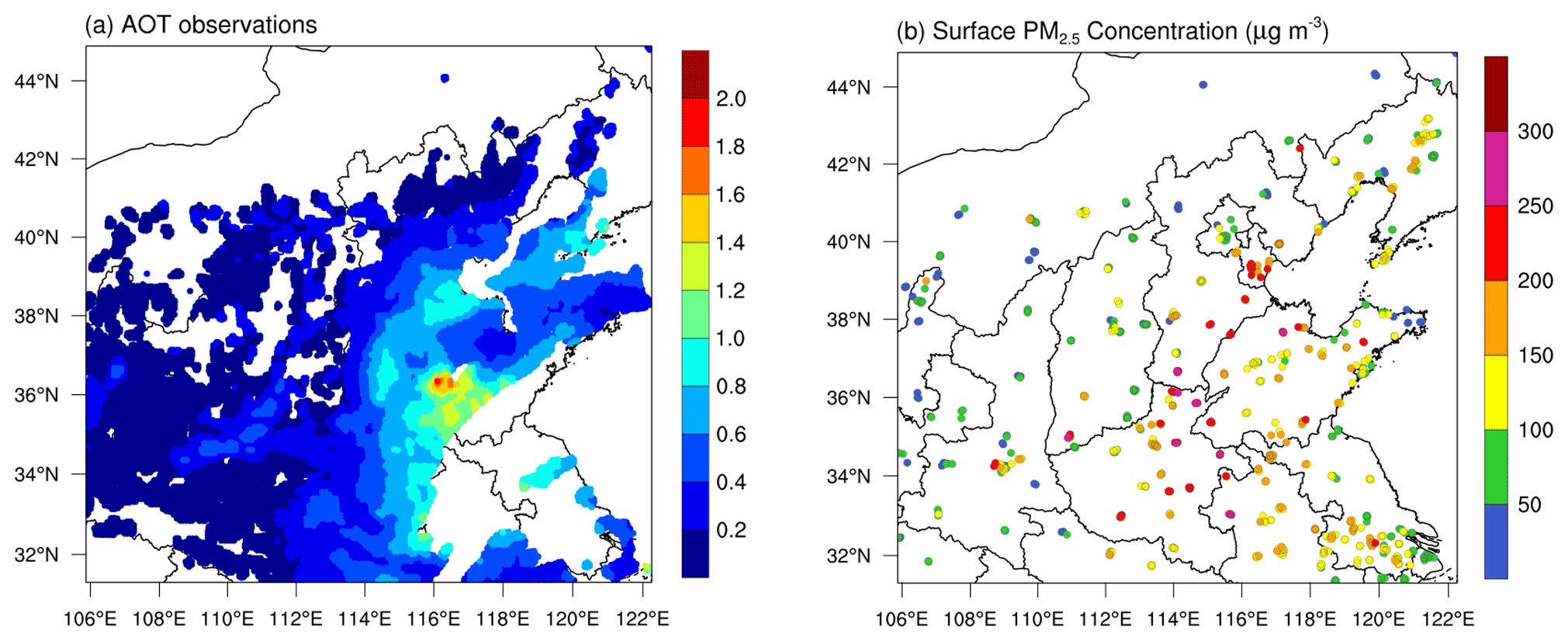
Figure 3 Observations of the thinned Himawari-8 AOTs (a) and surface PM_2.5 mass concentration (b) in D02 at 03:00 UTC on 25 November 2018.

The Himawari-8 AOT product was selected for assimilation by this system because it has a much higher temporal coverage than that of polar-orbiting satellites, which is promising for aerosol DA, and has also been successfully assimilated using other methods (Sekiyama et al., 2016; Yumimoto et al., 2016; Dai et al., 2019). The Himawari-8 level 2 AOT is retrieved at 500 nm with a 10 min observation interval and 0.05^∘ spatial resolution; however, the data are noticeably noisy. The level 3 AOT, including AOT_Pure and AOT_Merged, an improved hourly product, is an optimal estimation of AOT at a certain time rather than an estimate of the average state over an hour. AOT_Pure is a subset of level 2 AOT with strict quality control of cloud contamination, and AOT_Merged is the spatial and temporal optimum interpolation of AOT_Pure within an hour (Kikuchi et al., 2018). In this study, we focused on assimilating the latest version of the Himawari-8 level 3 AOT_Merged at 500 nm, which contains as many AOT retrievals as possible with a horizontal resolution of 0.05^∘ × 0.05^∘. The original AOT data are commonly thinned before directly assimilating to avoid seriously overestimated increments caused by the much higher spatial resolution of AOT data than that of the model (Yumimoto et al., 2016; Dai et al., 2019; Ha et al., 2020). Similar to Ha et al. (2020), we thinned the original AOT data over the D01 mesh (27 km) and D02 mesh (9 km), respectively, using the mean value of all the data points in one grid cell. A case of thinned AOTs retrieved at 03:00 UTC on 25 November 2018 in D02 is shown in Fig. 3a, the number of data is 13100, with a maximum value of 1.801. The AOT observations represent a heavy aerosol pollution episode that occurred in northern China, yet there is a lack of aerosol information in some heavily polluted regions due to cloud contamination, meaning that optical retrievals alone are not sufficient to thoroughly study aerosols. The Himawari-8 AOT is retrieved in the visible and near-infrared bands, so the observation coverage differs with time of day. Nevertheless, the observations at 03:00 UTC can nearly cover the whole of China (except some western areas). Hence, we chose the 03:00 UTC rather than 00:00 UTC, as used in usual experiments, as the initial time to perform a 24 h prediction of aerosols for the purpose of research.

To evaluate the performance of Himawari-8 AOT assimilation, three common statistical metrics, including the correlation coefficient (CORR), root-mean-squared error (RMSE), and mean bias (BIAS), were utilized (Boylan and Russell, 2006). It should be noted that compared with observations is the WRF-Chem D02 simulation, the results given below were computed using D02 outputs. First, we investigated the effects of AOT assimilation on AOT simulations using assimilated Himawari-8 AOTs and independent observations, including MODIS AOT and AERONET AOT observations. Second, we investigated the effects of assimilating AOTs on PM_2.5 analysis and forecasting using hourly surface mass concentration observations (Fig. 1b) released by the China National Environmental Monitoring Centre (CNEMC). For instance, the PM_2.5 mass concentration observed at 03:00 UTC on 25 November 2018 in D02 is shown in Fig. 3b, indicating a severe pollution zone in northern China, which is largely consistent with the spatial representation of Himawari-8 AOTs.

4 Statistics of background error covariance

Background error covariance is an important issue in data assimilation, which not only specifies the spread of observation information in the background field, namely the way in which the observations affect the background values, but also determines the relative weight of observational and background information across the analysis field. In practice, however, the error covariance B matrix is too large for a multi-variable aerosol DA to be calculated numerically. For instance, the number of D02 grid points used here is in the order of 10⁶, in addition to 20 state variables, the number of elements in B is, therefore, 10⁷ × 10⁷. This size will result in difficulty for computing and storing B, therefore a simplification of B is required. Following the studies of Bannister (2008) and Li et al. (2013), the B matrix was reduced to background error SD D, horizontal correlation matrix, and vertical correlation matrix, which can be computed separately. These three submatrices have dramatically fewer dimensions than B, and thus they become computationally treatable. Because the forecast error is unknown, most studies use model outputs to statistically estimate error covariance via modeling or parameterization, such as the National Meteorological Center (NMC) method (Parrish and Derber, 1992), which has been regularly used to calculate background error covariance for traditional meteorological fields such as temperature and wind and is also appropriate for aerosol mass concentrations (Benedetti and Fisher, 2007; Liu et al., 2011; Li et al., 2013). This study also utilizes the NMC method to calculate background error SDs, horizontal correlation, and vertical correlation based on differences between 48 and 24 h forecasts valid at the same time (i.e., 00:00 UTC) within a period of 1 month (November 2018). Because each aerosol state variable has a different background error covariance from others, which has been demonstrated by error statistics (see below), there is a need to estimate the error covariance for each variable to achieve better assimilation performance.

The error SD D matrix of each variable is diagonal and was directly estimated as a domain average at every model level using WRF-Chem D01 and D02 outputs, respectively, and its vertical distribution (only for D02) is shown in Fig. 4. These SDs differ among aerosol variables. In terms of values, SSN2, SSN3, OIN2, and OIN4 have larger error SDs than the others, with SSN2 having the largest value. The background error SDs are related to the aerosol species mass concentration. In general, variables with higher mass concentrations tend to have larger error SDs. For example, the simulation domain is far from the sea, and sea salt aerosols are very rare. As a result, no matter which size bin, the species CN has significantly lower error SDs below 0.05 µg m⁻³, which is much lower than the other variables. These error SDs display a relatively rapid decrease with height apart from SSN2 and SSN3​​​​​​​, but diminishing rates vary among aerosol variables. The fine structures of the error SD vertical distribution are related to the boundary layer heights. There is a noticeable increase in the SSN2 and SSN3 error SDs at the boundary layer height (approximately 1000 m).

Figure 4 Vertical profiles of background error SDs in mass concentration for aerosol control variables EC1, EC2, EC3, EC4, OC1, OC2, OC3, OC4, SSN1, SSN2, SSN3, SSN4, CN1, CN2, CN3, CN4, OIN1, OIN2, OIN3, and OIN4 in the data assimilation process, which were calculated using WRF-Chem D02 forecasts for 1 month, i.e., November 2018.​​​​​​​

The horizontal correlation matrix determines the propagation of observation information from the observation site to the surrounding area in the horizontal direction. Similar to Li et al. (2013), we assumed that different aerosol variables are not correlated; therefore, only auto-correlations of one variable at different distances were taken into consideration. For further simplification, we assumed that horizontal correlations are isotropic (Kahnert, 2008), which means that horizontal correlations are just a function of distance and have nothing to do with direction. Consequently, the horizontal correlation can be fitted using a one-dimensional Gaussian function. The correlation between two arbitrary points x₁ and x₂ can be expressed as $c(x_{\mathrm{1}},x_{\mathrm{2}})=\exp [-(x_{\mathrm{1}}-x_{\mathrm{2}}{)}^{\mathrm{2}}/\mathrm{2}{L}_v^{\mathrm{2}}]$, where L_v is the only unknown parameter and is the horizontal correlation length scale of each state variable. The correlation increases as the distance decreases, when the distance decreases to zero it obtains a maximum of 1. Thus, L_v is defined as the distance at which the correlation decreases to $e^{-\mathrm{1}/\mathrm{2}}$ and can be calculated via model outputs. This distance averaged over the model domain was used as an estimate of L_v. The introduction of L_v reduces the relatively complex two-dimensional correlation matrix to a parameter that is able to completely describe the structure of horizontal correlation, undoubtedly simplifying the computing and storage of the horizontal correlation matrix. The estimated L_v in D02 for individual aerosol state variable is given in Table 1. The estimated correlation length scales are significantly different among the distinct species. Thus, out of all aerosol variables, SSN3 has the largest scale at 47 km, indicating that the influence of SSN3 observations could spread farther than other variables and has a larger domain improvement across the background field. In contrast, CN3 has the smallest scale (12.8 km) and spreads the least based on observational information. Overall, SSN species have relatively large correlation length scales among species of the same size section, except for in the fourth bin. Additionally, the same aerosol species in different size sections have distinctly different error correlation length scales; for example, OIN3 has a larger scale than OIN2. Such differences among the correlation length scales indicate the need to use multi-species concentrations within the four size bins as control variables.

Table 1 Horizontal correlation length scales for individual aerosol state variables.

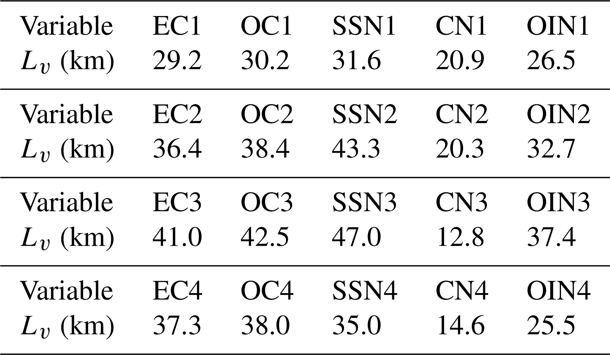
Figure 5 Vertical auto-correlations of background errors for aerosol state variables within the third size bin, i.e., EC3, OC3, SSN3, CN3, and OIN3. These statistics are directly estimated by the NMC method using WRF-Chem D02 outputs. Both axes are logarithmic and the contour interval is 0.1.

Background error vertical correlation plays an important role in the vertical spread of aerosol observation information. On the one hand, it has more complicated structures instead of isotropy compared to the horizontal correlation because of the discontinuity-like transition of the vertical distributions between the boundary layer and the free atmosphere above, and such structures are difficult to represent using an analytic function. On the other hand, the vertical correlation, which is the nz × nz (here, nz is equal to 40) matrix, is much smaller than the horizontal correlation matrix. As a result, the vertical correlation was directly estimated using model outputs. Because the vertical correlation of every variable is similar, the computed vertical correlations only for control variables in the third size bin are shown in Fig. 5. A salient and common feature of these vertical correlations is that they decrease with height and have strong relation to the boundary layer heights, which means that aerosols are mainly stacked in the boundary layer and tend to accumulate closer to the ground. At the same time, consistent with the horizontal correlations, vertical correlations differ among aerosol variables. SSN3 has a relatively large vertical scale, whereas CN3 has a relatively small vertical scale, which is consistent with the horizontal features.

5 Results

5.1 Effects on AOT simulations

AOT is of great value for studying aerosol activities, which can be simulated by the forward operator within the DA system. In general, assimilating AOT certainly improves its analysis according to the basic principle of the 3DVAR algorithm unless it is not successfully assimilated. It is noted that the wavelength variable necessary for computing AOTs described in Sect. 2.4 was set to be 500 nm, the wavelength at which the Himawari-8 AOTs are retrieved. A comparison between the simulated AOTs in the background field and analysis is usually employed to demonstrate the positive effects of assimilation. For illustration, the simulated AOTs and the so-called AOT increments at an initialization of 03:00 UTC on 25 November 2018 are shown in Fig. 6. The increments, which are differences between the analysis and the background field, can be considered the changes generated by assimilation, including magnitude and range, and these increments are spatially consistent with the observations, which means that the observations have an important effect on the assimilation results. Obviously, the simulated AOTs in the background field are dramatically underestimated (Fig. 6a) compared with the observed Himawari-8 AOTs (Fig. 3a), while the analysis brings the AOTs closer to the observations, which is indicated by the prominently positive increments (Fig. 6c). At the same time, assimilation also decreases the AOTs over other regions, with negative increments marked in blue. The background field is generally unable to describe the real pollution, especially in the case of heavy pollution; however, the analysis after assimilation can provide a relatively accurate pollution situation (Fig. 6b).

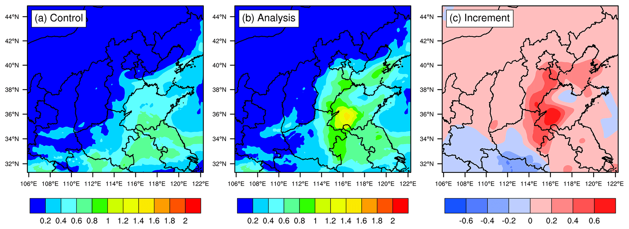
Figure 6 Spatial distributions of simulated AOTs in the background field (a) and analysis (b) and the increments (c), which are differences between the analysis and the background field. For illustration, distributions in D02 at a model initialization of 03:00 UTC on 25 November 2018 are given, which are similar to other results during the experiment period (i.e., from 23 to 29 November 2018).

Figure 7 Scatter plots of the simulated AOTs colocated in D02 vs. (a) the observed Himawari-8 AOTs and (b) Terra MODIS AOTs. These data were a set of all initializations from 23 to 29 November 2018; blue points are the control experiment, while red points are the assimilation experiment. The solid line is the 1 : 1 line where simulated values are equal to observed values, and the dashed lines correspond to 1 : 2 and 2 : 1.

The distributions shown in Fig. 6 express the effects of assimilating AOT on its analysis. To quantitatively evaluate the effects, the three metrics described above, CORR, RMSE, and BIAS, were computed through all the data pairs between the simulated and observed AOTs after spatial interpolation from regular grid points to the corresponding observational locations. Higher scores for the metrics CORR, RMSE, and BIAS would demonstrate better assimilation performance and vice versa. Besides, the assimilated Himawari-8 AOTs were used to compute the metrics, and another independent observation MODIS AOT was employed to fully evaluate the effects of assimilation on the analysis. The Terra MODIS level 2 AOT data (MOD04_L2) were used for validation in this study. As this polar-orbiting satellite passes over the Equator at 10:30 LT, we collected all the data between 00:00 and 06:00 UTC, rather than at a given time, to obtain more observations, matching the simulated values at the initial time (i.e., 03:00 UTC). It is worth mentioning that MODIS AOT is retrieved at 550 nm and the simulated AOT is at 500 nm, which will have a small and thus not largely significant effect on the evaluation. The experiment lasted for a week in cycles of 24 h, which contained seven initializations, and thus we gathered the simulated AOTs at all the initializations to achieve a general evaluation result. The comparisons between the observed and simulated AOTs are presented using scatter plots, as shown in Fig. 7, where Fig. 7a represents the comparison with Himawari-8 and Fig. 7b shows a comparison with MODIS. The comparison with Himawari-8 AOTs reveals that the analyses have a better performance as CORR increases from 0.524 to 0.868, RMSE decreases from 0.280 to 0.147, and BIAS is reduced by about 77 % after assimilation. Similar results are found in the comparison with the MODIS AOTs. Red points are distributed more densely and more parallel to the 1 : 1 line than the blue points, indicating that the analyses are closer to the observations. All three metrics demonstrated positive effects from assimilation on the analysis. Usually AOT at higher wavelengths (550 nm) is smaller than AOT at lower wavelengths (500 nm), and thus the bias would be even more negative if comparing AOT simulations with MODIS AOT for both control and analysis, which is demonstrated by the indicator BIAS in Fig. 7. For instance, BIAS is −0.031 when comparing with Himawari-8 AOT, while BIAS is −0.140 against MODIS AOT after assimilation. In summary, the assimilation system can successfully introduce AOT observations into the model to generate a more accurate initial field.

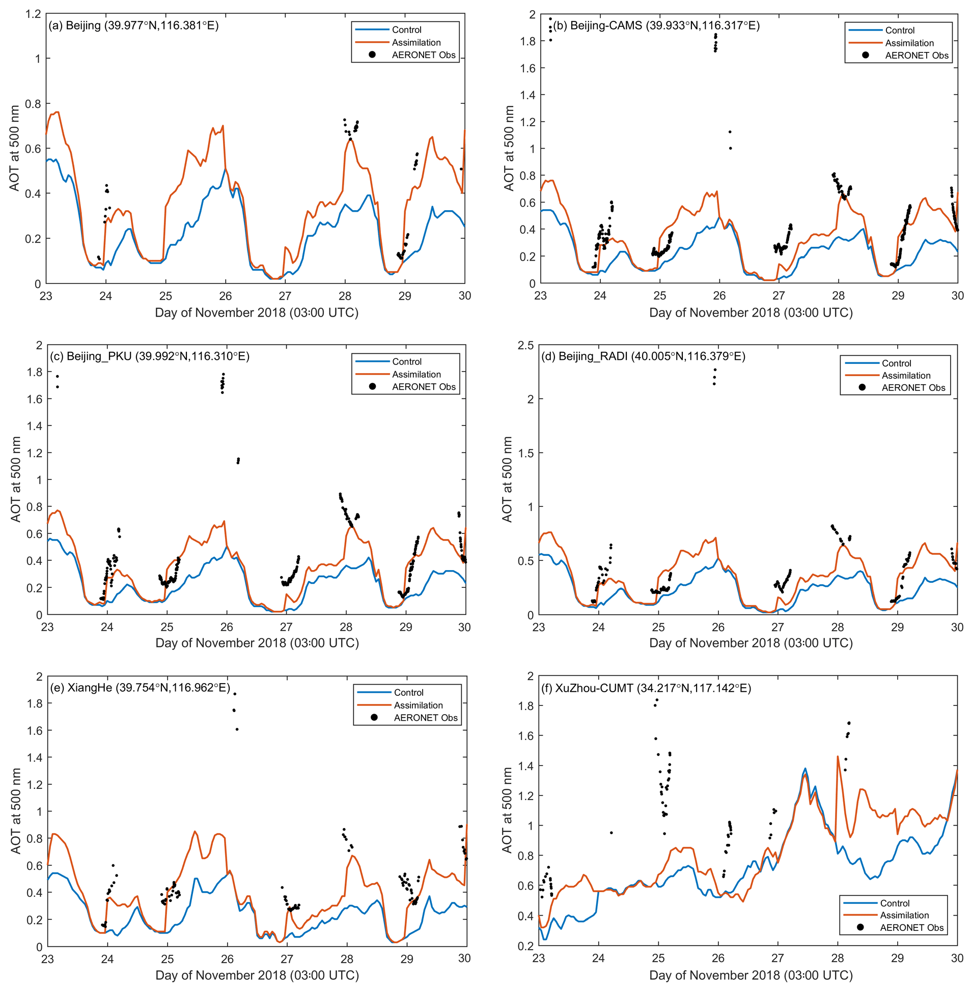
Figure 8 Time series of the simulated AOTs colocated in D02 and AERONET AOT observations at (a) Beijing, (b) Beijing-CAMS, (c) Beijing_ PKU, (d) Beijing_RADI, (e) XiangHe, and (f) Xuzhou-CUMT during the whole forecasting period. Both simulated AOTs and observed AOTs are at 500 nm. The brown line is the control experiment, while the light blue line is the assimilation experiment, and the AERONET observations are represented by black dots, which are only available under clear-sky conditions.

Similar to other studies (Dai et al., 2019; Ha et al., 2020), an independent validation of the simulated hourly AOTs from both the control and assimilation experiments was conducted through a comparison with AERONET observations to further investigate the effects of assimilation on forecasting. There are a total of six AERONET sites in D02: Beijing, Beijing-CAMS, Beijing_PKU, Beijing_RADI, XiangHe, and Xuzhou-CUMT, which are marked with red triangles in Fig. 1b. The sites can provide various AOT retrievals at different wavelengths, and those at 500 nm were selected for validation. In this study, we took level 2.0 and 1.5 (if level 2.0 data are not available) AERONET AOTs, which are cloud-screened (Smirnov et al., 2000), and used them to evaluate satellite observations. Figure 8 depicts the time series of the simulated AOTs and observations at six AERONET sites from 23 to 30 November 2018. Compared with observations, the control experiment dramatically underestimated AOTs at all sites, while the assimilation experiment significantly enlarged AOTs so that they became closer to the observations. This indicates that assimilation significantly improves AOT simulation. As can be seen, the assimilation benefits vary with sites; for instance, assimilation improves the AOT simulation, as well as the forecasting time, at Xuzhou-CUMT less than that at other sites (Fig. 8f); for example, the assimilation benefits for analyses can reach 24 h in the case of 25 November, while they last less than 24 h in the case of 24 November. The available observations largely account for this variation. A high-pollution event took place on 26 November in northern China so that AOTs over 1.6 were measured in Beijing (Fig. 8b), which can also be demonstrated by ground-level PM_2.5 observations (not shown here), but there are few Himawari-8 observations for the event to be assimilated due to cloud contamination. As a result, the assimilation experiment had the same performance as the control experiment, which is unable to describe the high-pollution event. It has been concluded that the introduction of AOT observations by assimilation is beneficial to capture heavy pollution levels (Rubin et al., 2017).

5.2 Effects on PM_2.5 simulations

PM_2.5 mass concentrations draw large attention from both the public and researchers. They can be directly modeled using WRF-Chem and are conventionally measured at ambient air quality monitoring stations. As the DA system was developed based on the MOSAIC scheme, it should hopefully improve aerosol analyses and subsequent forecasts, especially for PM_2.5. Northern China is located in D02 and is known for its high levels of air pollution; therefore, WRF-Chem D02 outputs were directly employed to investigate the effects of assimilating Himawari-8 AOTs on regional PM_2.5 forecasts.

Figure 9 Spatial distribution of surface PM_2.5 concentrations simulated at an initialization of 03:00 UTC on 25 November 2018 in (a) the control experiment and (b) the assimilation experiment and (c) the increment that is the difference between (b) and (a). These quantities are in units of µg m⁻³ and colocated in D02.

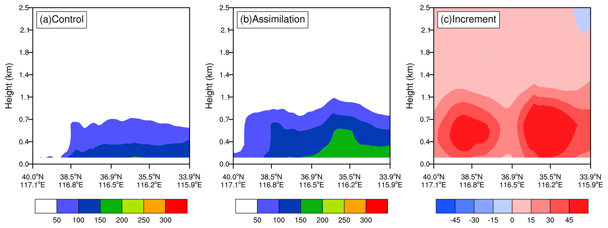
Figure 10 Vertical cross section of PM_2.5 in the background field (a), analysis (b), and the increment (c) in D02 at 03:00 UTC on 25 November 2018.

As described in Sect. 2.3, the assimilation process will produce the increments of 20 control variables. Of course, we can analyze every increment to assess the effects of AOT assimilation on the corresponding aerosol species simulations. Because there is a lack of observations for aerosol species at each size section, the total increment of PM_2.5 is analyzed instead, which is simply a summation of increments over five assimilated species in the first, second, and third size bins. For illustration, Fig. 9 only shows the simulated surface PM_2.5 concentrations in the background field and corresponding analyses at an initialization of 03:00 UTC on 25 November 2018, as well as the increments. The control experiment underestimated PM_2.5 concentrations in northern China compared with the observed values (Fig. 3b). For example, the PM_2.5 concentrations in Tianjin marked by the small black triangle in Fig. 9 reached more than 200 µg m⁻³, while the simulated values in the background field were less than 150 µg m⁻³ (Fig. 9a). The evidently positive increments generated by assimilation enlarge PM_2.5 analyses (Fig. 9c), making them closer to the observations, and the analyses are therefore able to describe heavy pollution. At the same time, negative increments decrease overestimation in some places. The PM_2.5 increments are spatially consistent with AOT observations (Fig. 3a), which means that aerosol optical properties have been transformed into mass concentrations using the observation operator and then incorporated into the model. The analyses are superior to the background field in terms of pollution magnitude; however, the heavy pollution band in northern China was simulated further to the east compared with the observations. This might be ascribed to model deficiency in the representation of three-dimensional aerosol species. Since AOT is an atmospheric column measurement, it naturally includes the information of aerosol vertical distributions. Consequently, AOT assimilation can improve aerosol vertical distributions as well. A vertical cross section of PM_2.5 at 03:00 UTC on 25 November 2018 is shown in Fig. 10; this cross section is through Tianjin. Similar to surface PM_2.5, suspended PM_2.5 mass concentrations in the upper air are also enlarged with a wide range from the ground to about 1 km by significantly positive increments generated by assimilation (Fig. 10c). Despite having no observational PM_2.5 profiles to compare it with, the vertical distribution in analyses is believed to be closer to the real distribution in terms of the ground PM_2.5 level (Fig. 10b). It should be noted that the vertical increments are determined by the background error vertical correlation. In summary, AOT assimilation is certainly helpful to improve the three-dimensional descriptions of PM_2.5.

Assimilation directly aims to improve aerosol analyses. As shown in Fig. 11, the data dots between simulated and observed PM_2.5 concentrations were also analyzed according to the three metrics. From Fig. 11, the red points (standing for analyses) do not have a significantly better performance than their blue counterparts for the control experiment, yet the metrics demonstrate the slight positive effects of AOT assimilation on aerosol analyses, increasing CORR from 0.485 to 0.530, decreasing RMSE from 60.66 to 56.40 µg m⁻³, and reducing BIAS by 4.97 µg m⁻³. This improvement is less significant than that of directly assimilating PM_2.5 concentrations (Wang et al., 2020); however, the use of PM_2.5 concentrations to evaluate the effects of AOT assimilation is not objective and comprehensive because there is a discrepancy between PM_2.5 and AOT observations. For example, no assimilation benefits in some highly polluted areas are generated because of the lack of AOT retrievals, and thus the PM_2.5 observations cannot reflect the benefits from AOT assimilation. Besides, AOT is an atmospheric column measurement while PM_2.5 is a surface measurement. Therefore, if you have an aerosol plume that is not close to the surface, AOT can be increased by increasing the aerosol concentration of that plume, whereas PM_2.5 can remain almost unaffected by that change.

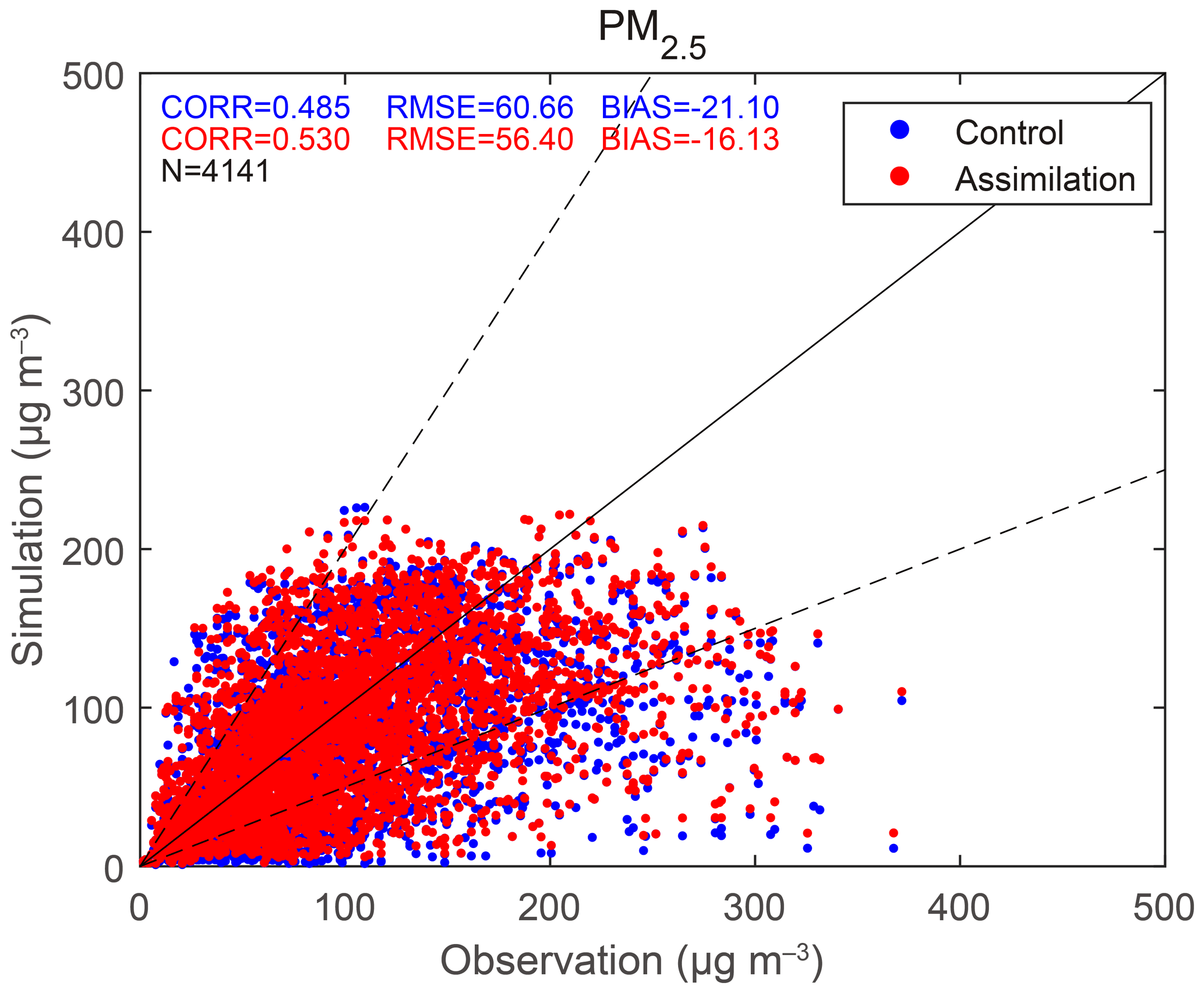
Figure 11 Scatter plots of the simulated PM_2.5 concentrations in the control experiment and corresponding analyses in the assimilation experiment vs. the observations. Like Fig. 7, these data are also colocated in D02 and a set of all initializations. Blue points stand for the control experiment, while red points stand for the assimilation experiment.

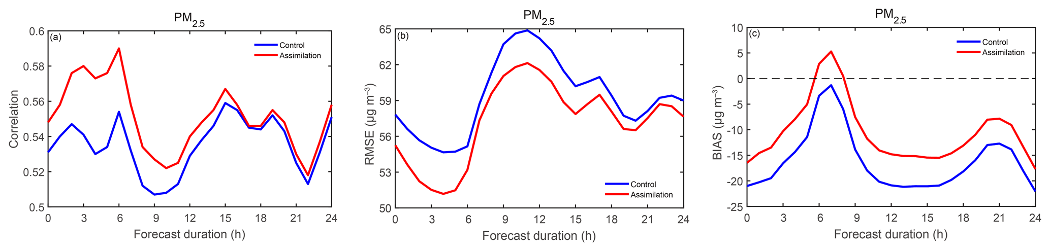
Figure 12 Statistical metrics (a) CORR, (b) RMSE, and (c) BIAS for surface PM_2.5 forecast performances in D02 regarding the forecast range, which are computed as an average over seven analysis steps. The blue line is the control experiment, and the red line is the assimilation experiment.

To investigate the effects of AOT assimilation on PM_2.5 forecasts, time series of three metrics regarding the forecast range (i.e., 24 h) were computed using hourly WRF-Chem D02 outputs and observations. As shown in Fig. 12, in terms of both CORR and RMSE, the assimilation experiment performed better than the control experiment, indicating that the benefits for analyses from AOT assimilation can last up to 24 h. It is noted that the assimilation benefits vary with integration time, decreasing in a fluctuating manner. The computed BIAS indicates that AOT assimilation improves PM_2.5 forecasts within 24 h but can vary for certain times. As discussed above, assimilation significantly enlarges the simulated PM_2.5 concentrations, but an overcorrection, namely that the simulated values surpass observations, occurs approximately 7–8 h from the initial time (Fig. 12c), which may be ascribed to the dramatically noisy AOT retrievals, as well as an imperfection of the observation operator for aerosol optical properties.

The time series of the simulated PM_2.5 concentrations and observations during the entire experimental period are shown in Fig. 13, which are hourly averaged over 683 stations in D02. The blue line denotes the control experiment, the red line denotes the assimilation experiment, and the observations are represented using the black line. Overall, the mean PM_2.5 concentrations simulated by the assimilation experiment were closer to the observations than the control experiment, which is beneficial for describing the real heavy pollution in northern China. Statistically, the CORR, RMSE, and BIAS between the black curve and blue curve were 0.645, 20.74 µg m⁻³, and −16.25 µg m⁻³, respectively, while CORR, RMSE, and BIAS between the black curve and the red curve were 0.732, 15.12 µg m⁻³, and −9.81 µg m⁻³, respectively, which means that the assimilation experiment had a better performance in PM_2.5 forecasts than the control experiment. These metrics indicate that AOT assimilation improves regional PM_2.5 forecasts, especially in the case of heavy pollution.

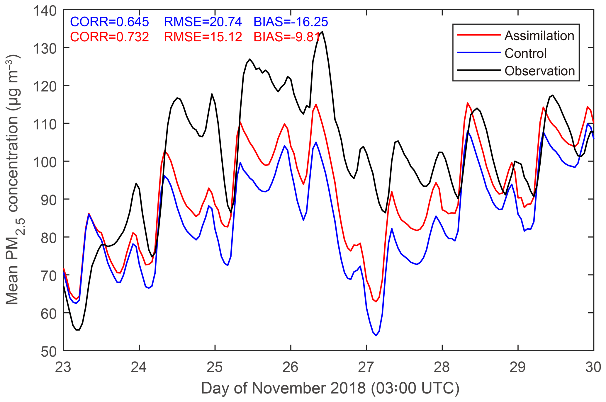
Figure 13 Time series of surface PM_2.5 simulated by the control experiment (blue) and the assimilation experiment (red) as well as corresponding observations (black), as averages over 683 stations in D02. The simulations are representative of hourly 0–23 h forecasts in D02 from 03:00 UTC every day during the whole forecasting period using WRF-Chem.

6 Summary and discussions

A 3DVAR DA system was independently developed to directly assimilate aerosol optical properties. This system was built based on the framework of Li et al. (2013) and developed for the MOSAIC scheme within WRF-Chem, a sophisticated aerosol model, rather than the GOCART scheme employed by CRTM. MOSAIC divides aerosol particles into eight species that are described in four size bins so that there are 32 mass concentration model variables. For computational efficiency, the 32 model variables were lumped into 20 aerosol state variables, which are representative of the mass concentrations of five assimilated species within the four size bins. An optical module was added to assimilate aerosol optical properties, which consisted of the forward observation operator and its TL and AD codes. We properly reduced the OP module (Fast et al., 2006) in WRF-Chem to establish the forward operator, then the TL and AD codes were generated using an automatic differentiation tool and tested to ensure that they were correct. The system can (simultaneously or separately) assimilate aerosol optical properties such as extinction coefficient profiles, AOTs, and mass concentrations, and these should be applied for further studies in the future.

Himawari-8 AOTs were assimilated to validate the system and investigate the effects of assimilation on both AOT and PM_2.5 simulations. A heavy air pollution event occurred in northern China from 23 to 29 November 2018; therefore, this period was chosen for the simulation experiment. Two comparative experiments with a spin-up time of 24 h were performed, continuously lasting for a week with a cycle of 24 h. The control experiment took the previous 24 h aerosol forecasts as an initialization, while the assimilation experiment employed analyses after assimilating Himawari-8 AOTs to initialize the simulations. WRF-Chem D02 outputs were compared with the assimilated AOTs, independent MODIS AOTs, AERONET AOT observations, and surface PM_2.5 mass concentration observations.

Background error statistics, including SDs, horizontal correlation length scales, and vertical correlations of 20 control variables, were estimated using monthly WRF-Chem outputs based on the NMC method, which are also necessary for the assimilation process. Our results showed that background error statistics distinctly vary among these control variables, which also illustrates the necessity of building a multi-variable aerosol DA system.

Assimilation significantly improves AOT analyses and forecasts. In general, the control experiment without assimilation seriously underestimated AOTs compared with the observed values. The analyses perform better in terms of the statistical metrics CORR, RMSE, and BIAS in comparison with both assimilated and independent AOTs than the background field. The analyses closer to observations improve AOT simulations, which is of great value in the study of AOT distribution during high-pollution events. The improvement in AOT simulations indicates that the system successfully assimilated AOT observations into the model to form an accurate initial field.

Subject to the basic formulation, the DA process directly aims to improve aerosol analyses. In terms of statistical metrics, assimilating Himawari-8 AOTs improves PM_2.5 analyses (but not significantly); in D02 and the assimilation benefits can last more than 24 h. Assimilation significantly enlarges the underestimated PM_2.5 concentrations to be closer to the real distribution in northern China during heavy pollution. The averaged surface PM_2.5 concentrations over D02 were better simulated during the whole pollution period after assimilation compared with corresponding observations, which means that AOT assimilation improves regional PM_2.5 simulations.

In this study, the observation errors of AOT retrievals were simply set as a constant. However, they should be determined by the retrieval uncertainty, or should be variable at least. Additionally, different thinning schemes for AOT retrievals may have different results. Consequently, these questions should be studied further. As more aerosol optical property observations become available, combined assimilation of optical properties and routine observations, such as aerosol extinction profiles and mass concentrations, has become popular. As described above, the system developed in this study has great potential for assimilating various observations. Assimilating AOTs here is a preliminary study, and combined assimilation studies should be performed in the future.