Calibrating the soil organic carbon model Yasso20 with multiple datasets

Soil organic carbon (SOC) models are important tools for assessing global SOC distributions and how carbon stocks are affected by climate change. Their performances, however, are affected by data and methods used to calibrate them. Here we study how a new version of the Yasso SOC model, here named Yasso20, performs if calibrated individually or with multiple datasets and how the chosen calibration method affects the parameter estimation. We also compare Yasso20 to the previous version of the Yasso model. We found that when calibrated with multiple datasets, the model showed a better global performance compared to a single-dataset calibration. Furthermore, our results show that more advanced calibration algorithms should be used for SOC models due to multiple local maxima in the likelihood space. The comparison showed that the resulting model performed better with the validation data than the previous version of Yasso.

1 Introduction

Soils are the second-largest global carbon pool, and hence even small changes in this pool impact the global carbon cycle (Peng et al., 2008). However, soil organic carbon (SOC) and associated changes are difficult and laborious to measure (Mäkipää et al., 2008). They can also vary drastically over space due to differences in litterfall, site, and soil type as well as climate (Jandl et al., 2014; Mayer et al., 2020). Hence, SOC models are important tools for estimating current global soil carbon stocks and their future development (Manzoni and Porporato, 2009). Numerous SOC models have been developed in the past decades (Parton, 1996; Camino-Serrano et al., 2018; Thum et al., 2019) to quantify the global SOC stocks and estimate the effects of different drivers, such as changing environmental conditions, on SOC stocks (Sulman et al., 2018; Wiesmeier et al., 2019).

While the majority of SOC models rely on linear equations representing the movement of C within the soil, there have been studies showing the need to represent at least some of the SOC processes such as the microbial influence by non-linear equations (Zaehle et al., 2014; Liang et al., 2017) or that the state structure of the model affects what kind of data can be used to calibrate it (Tang and Riley, 2020). More complicated SOC models addressing these arguments have been developed, for example Millennial (Abramoff et al., 2018), and modules including additional drivers affecting the C pools have been included in existing SOC models, such as nitrogen (Zaehle and Friend, 2010) and phosphorus (Davies et al., 2016; Goll et al., 2017) cycles. Their implementation is hindered, though, by the fact that detailed data are needed to constrain the model parameterization, but individual measurement campaign datasets are often limited in size and lacking in nuance of the SOC state (Wutzler and Reichstein, 2007; Palosuo et al., 2012). Consequently, multiple datasets representing different processes should be used to parameterize the models in order to capture the multitude of SOC dynamics, but combining observation datasets with varying spatial scales, measurement temporal densities, inherent assumptions, and structural errors can cause issues with adequately incorporating all the information (Oberpriller et al., 2021). The chosen calibration methodology is additionally affected by the same issues based on its approach of fitting the data.

Litter-bag decomposition experiments (Harmon et al., 2009) provide information on the faster decomposition processes, but their applicability to longer-term assessments has been questioned (Moore et al., 2017). Furthermore, even in current studies it is common to use only data from one litter-bag decomposition experiment campaign (for example Kyker-Snowman, 2020) due to the differences in experimental setups and physical properties of the litter bags, making direct comparison of results difficult. Organic carbon content can be measured from soil samples, but those measurements provide a limited snapshot because of the large number of measurements needed to detect changes and the slow dynamics of SOC (Mayer et al., 2020). Additionally, the SOC in these measurements cannot effectively be fractionated into different state components used in the models. Hence, assumptions need to be made on the amount of short-lived SOC to approximate the amount of long-lived SOC. There are also other aspects of litter that are known to affect the decomposition rate, e.g. the bigger the size of the woody litter the slower the decomposition is (Harmon et al., 2000), which requires detailed and specific observations to inform models.

The Yasso07 model (Tuomi et al., 2009) was developed to address some of these challenges. In it, both the litter inputs and the soil carbon are divided into chemically measurable fractions that decompose at their own rate, which are affected by environmental conditions, specifically ambient temperature and moisture. This direct link between the model state and litter input allowed using different litter decomposition experiment data to constrain model parameters. One of the core ideas in the development of Yasso07 is that the parameterization process itself is done simultaneously with multiple datasets reflecting different parts of the SOC decomposition process in a Bayesian calibration framework (Zobitz et al., 2011). As a part of this approach, a litter-bag-specific leaching term was introduced in order to be able to use information from several litter-bag experiments at the same time (Tuomi et al., 2011b).

While the initial Yasso07 calibration addressed challenges regarding the variety of data required, it did not touch in detail on the issues affecting the actual SOC model parameterization process. First, Yasso07 did not calibrate all the parameters simultaneously with all the data, but instead calibrated the parameters in segments for which the previously calibrated parameters were set as constant when calibrating the next set of parameters (Tuomi et al., 2011a). While this makes the calibration process easier, it naturally also affects the results and associated uncertainties. Second, there have been no standard methods established to evaluate how the inclusion of additional datasets impacts the general performance of SOC models. In other words, does using multiple datasets improve the model estimates? Naturally, this applies to Yasso07 as well. Third, there have been studies which indicate that the choice of parameterization method does matter in ecosystem modelling (Lu et al., 2017). It is reasonable to assume that this would also hold true for SOC systems wherein there could be multiple parameter sets that can potentially produce a local fit into the data. Last, but not least, the previous Yasso07 calibration workflow was not easily repeatable and reproducible to allow inclusion of new datasets and algorithms.

In this study, we built upon previous Yasso developments to present a model formulation that expanded on how the environmental drivers affect the decomposition. The data used to calibrate the model are the same for both versions with the exception of the measurement data regarding long-term carbon allocation. For Yasso07, a time series dataset from southern Finland was used, while for Yasso20, approximated steady-state SOC measurements from across the world were used to constrain the relevant parameters. Additionally, we use a more advanced model calibration method in association with a stricter protocol on what kind of data points were used for calibration and an open-source R package for data inclusion, repetition, and reproduction of calibration. The model and produced parameter set will be referred to as Yasso20 hereinafter. Our redesigned calibration protocol leverages the BayesianTools R package (Hartig et al., 2019), an open-source general-purpose tool for Bayesian model calibration. Using BayesianTools in our workflow, we not only established a more reproducible and standardized application of Yasso20 calibration, but also leveraged interfacing with multiple calibration algorithms and examined the role of the calibration method.

Due to the nature of the available SOC-related datasets we hypothesize the following: (i) the SOC model performs better globally if multiple datasets are simultaneously used to constrain it compared to a SOC model calibrated with an individual dataset despite the numerous assumptions required for combining the different information; (ii) the likelihood space created by these multiple datasets is uneven with multiple maxima to the degree that more advanced parameter methods are necessary for the end result not to be dependent on the starting point; and (iii) these changes in the model formulation and the calibration protocol will improve how the Yasso model projections perform compared to the previous model version.

The first hypothesis is tested by calibrating Yasso with individual datasets as well as the combined datasets with the resulting performances compared using numerous validation datasets. All these calibrations are done for all the parameters simultaneously. The second hypothesis is tested by comparing the Yasso parameter values produced by parameter estimation methods of varying complexity and how well they converge. Furthermore, the more extensive calibration process has allowed constraining more details in the new Yasso formulation, which is introduced here as well.

2 Methods

2.1 Yasso model description

The Yasso model is based on four basic assumptions on litter decomposition and soil carbon cycle: (1) litter consists of four groups of organic compounds (sugars, celluloses, wax-like compounds, and lignin-like compounds) that decompose at their own rate independent of origin (Berg et al., 1982). (2) Decomposition of any group results either in formation of carbon dioxide (CO₂) or another compound group (Oades, 1988). (3) The decomposition rate is affected by environment temperature and moisture (Olson, 1963; Meentemeyer, 1978; Liski et al., 2003). (4) The diameter size of woody litter determines the decomposition rate (Swift, 1977). Yasso20 is the next version of Yasso (Liski et al., 2005) and Yasso07 models (Tuomi et al., 2009, 2011b) and continues to build on these same assumptions. The main formulation contribution in Yasso20 compared to the previous versions is the added nuance in how climate drivers affect the different pools, which in turn is possible here due to the improved calibration scheme. For the purposes of the calibration here, another assumption was necessary: (5) the most stable soil carbon compounds are only formed in the soil as a result of bonding with mineral surfaces (Stevenson, 1982). The following model formulations apply for Yasso20.

Based on the previously established assumptions, litter can be divided into four fractions according to its chemical composition. Compounds soluble in a polar solvent (water) represent sugars (W), and those soluble in a non-polar solvent (ethanol or dichloromethane) represent wax-like compounds (E). Compounds hydrolysable in acid (for example, sulfuric acid) represent celluloses (A), and the non-soluble and non-hydrolysable residue represents lignin-like compounds (N). Additionally, there is a fifth compartment, humus (H), which represents long-lived, stable soil organic carbon produced by interaction with mineral compounds in the soil. As the carbon compounds are broken down by the decomposition processes, they become either new compounds belonging to another compartment or CO₂. The decomposition rate of each compartment is considered independent of the litter origin and is affected by a temperature, moisture, and size component.

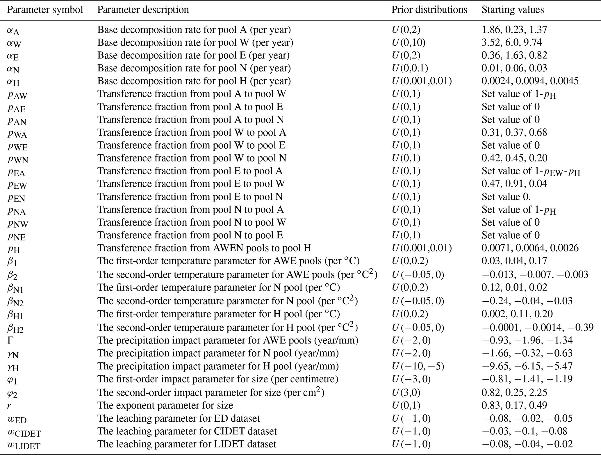
Table 1 The parameters, prior distributions, and initial values used in this calibration study. The initial values for the different chains were randomly drawn from the prior distribution (U: uniform). If the starting value is listed as a set value, then the parameter was not varied in the calibration and the given value was used for all chains.

The masses (x) of the compartments at time t are denoted by vector $\mathit{x}\left(t\right)=\left[x_{\mathrm{A}}\right(t),x_{\mathrm{W}}(t),x_{\mathrm{E}}(t)$,  x_N(t),  x_H(t)]. The Yasso model uses an annual time step and determines the changes in those masses according to

$$\begin{array}{}\text{(1)}& {\displaystyle \frac{\partial \mathit{x}\left(t\right)}{\partial t}}=M\left(\mathit{\theta },c\right)\mathit{x}{\left(t\right)}^T+b\left(t\right),\end{array}$$

where b(t) is the litter input to the soil at the time t, θ is the set of parameters driving decomposition as defined in Table 1, and c contains the factors controlling the decomposition. Not only are accurate soil moisture estimates challenging to obtain for the measurements used here, but a vast majority of them are from the surface. Thus, air temperature T and precipitation P were used as the environmental drivers along with the woody litter diameter d. Operator M is the product of the decomposition, as presented by K, and mass fluxes between compartments, as depicted by F:

$$\begin{array}{}\text{(2)}& {\displaystyle }M\left(\mathit{\theta },c\right)=F\left(\mathit{\theta }\right)K\left(\mathit{\theta },c\right),\text{(3)}& {\displaystyle }F\left(\mathit{\theta }\right)=\left[\begin{array}{ccccc}-\mathrm{1}& p_{\mathrm{WA}}& p_{\mathrm{EA}}& p_{\mathrm{NA}}& \mathrm{0}\\ p_{\mathrm{AW}}& -\mathrm{1}& p_{\mathrm{EW}}& p_{\mathrm{NW}}& \mathrm{0}\\ p_{\mathrm{AE}}& p_{\mathrm{WE}}& -\mathrm{1}& p_{\mathrm{NE}}& \mathrm{0}\\ p_{\mathrm{AN}}& p_{\mathrm{WN}}& p_{\mathrm{EN}}& -\mathrm{1}& \mathrm{0}\\ p_{\mathrm{H}}& p_{\mathrm{H}}& p_{\mathrm{H}}& p_{\mathrm{H}}& -\mathrm{1}\end{array}\right],\text{(4)}& {\displaystyle }K\left(\mathit{\theta },c\right)=\text{diag}.\end{array}$$

Here, parameters $p_{ij}\in [\mathrm{0},\mathrm{1}]$ denote the flows from compartment i(i∈{A,W,E,N}) to j(j∈{A,W,E,N,H}) and are included in the parameter vector θ. The decomposition rates k_i(θ,c) were calculated according to

$$\begin{array}{}\text{(5)}& k_i\left(\mathit{\theta },c\right)={\displaystyle \frac{{\mathit{\alpha }}_i}{J}}h\left(d\right)\left(\mathrm{1}-e^{{\mathit{\gamma }}_{i}P}\right){\sum }_{j=\mathrm{1}}^J{e}^{{\mathit{\beta }}_{i\mathrm{1}}{T}_j+{\mathit{\beta }}_{i\mathrm{2}}{T}_j^{\mathrm{2}}},\end{array}$$

where the base decomposition rate α_i, temperature parameters β_i1 and β_i2, and precipitation parameter γ_i for compartments i∈{A,W,E,N,H} are all a part of the parameter set θ. The temperature- and precipitation-dependent rate parameters are the same for compartments AWE, but both N and H compartments are given their own separate parameter values. In order to capture the annual temperature cycle more efficiently, the average monthly temperatures for all 12 months are given as an input with the model averaging over their impacts as seen in Eq. (5). The total annual precipitation is used instead of monthly precipitation as seasonal variation such as snowfall or heavy rainfall followed by long dry stretches would hinder the calibration if the monthly precipitation was used. The temperature and precipitation equations are established in Tuomi et al. (2008). Woody litter decomposition rate in response to diameter (d) is described in h(d) based on Tuomi et al. (2011a) as follows:

$$\begin{array}{}\text{(6)}& h\left(d\right)=min\left({\left(\mathrm{1}+{\mathit{\phi }}_{\mathrm{1}}d+{\mathit{\phi }}_{\mathrm{2}}{d}^{\mathrm{2}}\right)}^r,\mathrm{1}\right),\end{array}$$

where φ₁, φ₂, and r are parameters included in the parameter set θ.

Given initial state x₀, average environmental conditions c, and constant litter input b(t)=b, the model prediction can be computed by solving the differential equation in Eq. (1). The solution becomes

$$\begin{array}{}\text{(7)}& \mathit{x}\left(t\right)=M{\left(\mathit{\theta },c\right)}^{-\mathrm{1}}\left(e^{M\left(\mathit{\theta },c\right)t}\left(M\left(\mathit{\theta },c\right)x_{\mathrm{0}}+b\right)-b\right),\end{array}$$

where the matrix exponential is determined numerically. In a steady-state situation $x={lim}_{t\to \mathrm{\infty }}x\left(t\right)$, Eq. (7) becomes

$$\begin{array}{}\text{(8)}& x=-M{\left(\mathit{\theta },c\right)}^{-\mathrm{1}}b.\end{array}$$

Yasso20 improvements

Two main changes were introduced to the Yasso20 version here compared to the earlier Yasso07 version. The first change was that the temperature input for Yasso20 is given as the mean monthly temperature for each month of the year instead of the mean annual temperature and associated annual temperature amplitude. This was done in order to better represent the more nuanced global temperature profiles.  For example, the previous scheme was indifferent to whether the winter was long or short, which is expected to affect the annual decomposition. The second change was to differentiate the climate driver impacts between the AWE, N, and H pools instead of using the same parameter values for all the model C pools. This was done because previous research established that more complex carbon compounds require more energy to be broken up (Davidson and Janssens, 2006), which indicates that the parameters representing those dynamics should also differ between pools. It is expected that these changes will affect the model performance and the calibration results themselves, especially as this allows the environmental conditions to impact the pools differently. Thus, this changed model version was determined to be a new version of the model. We do not compare Yasso20 performance to Yasso07 here. All model parameters given in Table 1 were targeted in the calibration.

2.2 Datasets used in the calibration

Several datasets were simultaneously used to calibrate the model in order represent different processes related to soil carbon cycling: decomposition bag time series data from the Canadian Intersite Decomposition Experiment (CIDET; Trofymov and the CIDET Working Group, 1998), the Long-Term Intersite Decomposition Experiment (LIDET; Gholz et al., 2000) and European Intersite Decomposition Experiment (ED; Berg et al., 1991a, b) projects, a collection of global soil organic carbon measurements gathered by Oak Ridge National Laboratory (Zinke et al., 1986), and a woody matter decomposition dataset from Mäkinen et al. (2006). In addition to these large datasets, a smaller litter-bag decomposition dataset from Hobbie et al. (2005) was used to evaluate how much the addition of a comparatively small number of data points affects the calibration results and an independent validation dataset for the other calibration parameters. These datasets along with additional details are listed in Table 2.

Table 2 The measurement datasets used in this research.

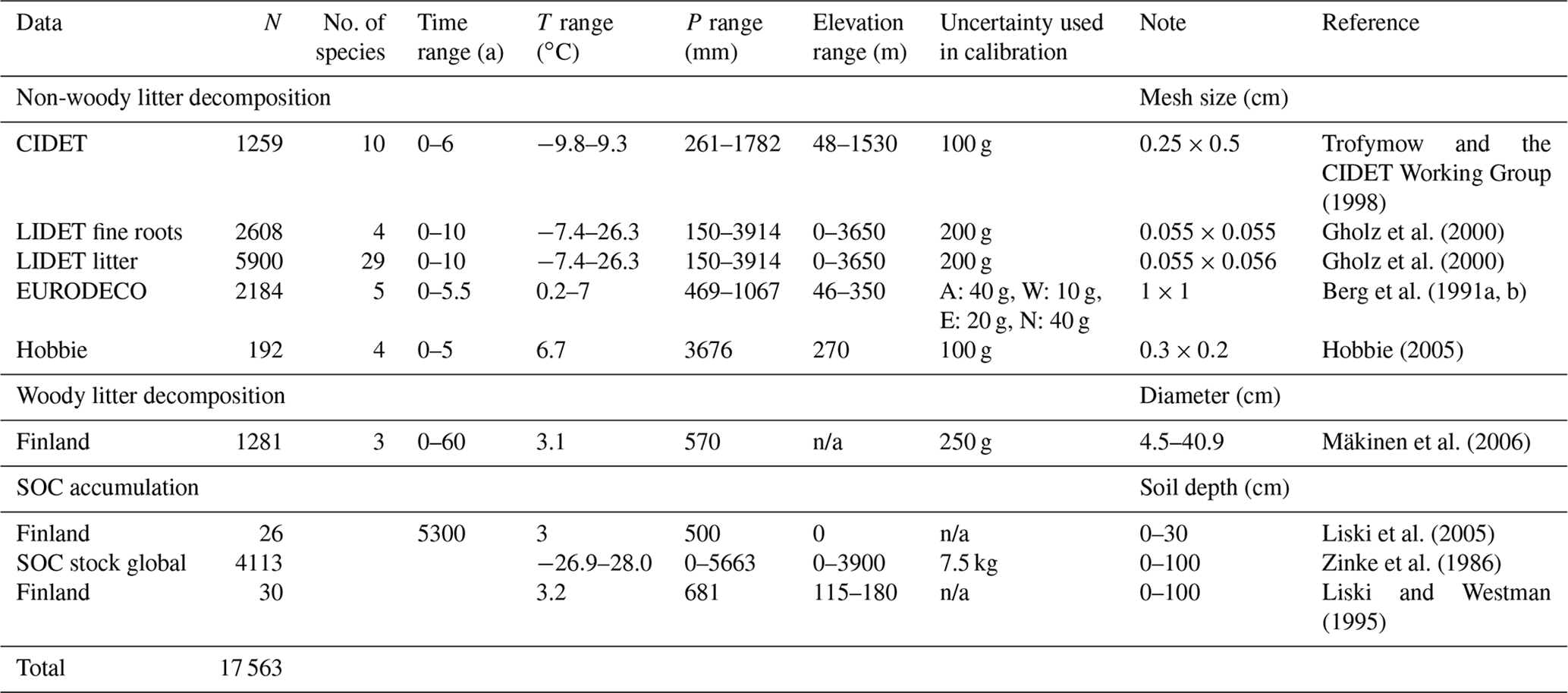
n/a: not applicable

CIDET, LIDET, and ED are litter-bag decomposition time series with litter left to decompose in a mesh bag and the remaining mass measured at chosen time intervals over several years. Each dataset had the experiments with multiple different species, with the initial chemical composition also provided by the dataset, and different sites. Furthermore, while CIDET and LIDET only measured the remaining mass, ED also determines the AWEN fraction from one of the replicant samples, which allows us to directly compare it to the Yasso20 state variables. However, while in CIDET and LIDET the remaining mass has ash removed, in ED ash is still included in the remaining mass. The mean monthly temperatures and precipitation have been measured at each test site with the annual precipitation being summed up from the monthly precipitation values.

The global SOC measurement dataset from Oak Ridge National Laboratory (Zinke et al., 1986) is a collection of data from numerous unrelated projects that have measured SOC as a part of their campaign. As such, there are no uniformly applicable protocols for these measurements. For the purposes of the calibration, the data are assumed to represent the steady-state SOC at that location and each measurement is treated as independent from the others even if they are from the same location. Furthermore, we only used SOC measurements that were below 20 kg C m⁻² in the calibration. Values higher than those were found in high latitudes and considered to be results of waterlogging, peat formation, or permafrost, which are processes not described in Yasso20. The litter input was determined by combining the global gross primary production (GPP) map from Beer et al. (2010) with the global NPP–GPP (NPP: net primary production) relationship set to 0.5 at the measurement locations due to lack of specific information on the NPP–GPP there. The Olson classification (Olson et al., 2001) regarding the local ecosystem type was used to roughly divide the ecosystems into grasslands, semi-forests, and forests. The litter fractioning for these different systems is given in Table S1. In addition, SOC chronosequence data from Liski et al. (1998) and plot-level measurements of Liski and Westman (1995) were used as a validation dataset.

The woody decomposition data used here are from Mäkinen et al. (2006), which include measurements of multiple trees in different stages of decomposition over several decades in Finland. There are no signifiers to connect the measurements from different years or to indicate how much the tree diameter has been reduced over time because the data were not chronosequence data for the same trees. As such, the measurements were considered independent and representative of decomposition of a tree trunk of that size.

The same litter-bag and woody data were used to calibrate both Yasso07 and Yasso20. The sole exception regarding the litter-bag data is that the whole ED dataset was used in Yasso07 calibration, while in Yasso20 we removed decomposition data from manipulation experiments. However, Yasso07 H pool parameters were not parameterized with the Oak Ridge data. Instead, the chronosequence data from Liski et al. (1998) were used in its calibration with climate and litterfall drivers derived from southern Finland conditions (Tuomi et al., 2009). As already established, this dataset was not used in Yasso20 calibration and was only applied as a validation dataset.

Dataset uncertainties

The information on the uncertainty related to the measurements was limited. With CIDET and LIDET there are generally four replicants, sometimes fewer, from which the standard deviation in remaining mass can be calculated. Similar standard deviation is available for the ED measurements, but it is only determined for the total mass loss and not for the AWEN pool measurements used here. Furthermore, there are other aspects affecting the uncertainties such as the ED measurements containing ash or LIDET measurement time series showing more noise than the CIDET measurements. For the global SOC dataset and the woody matter decomposition datasets no such replicant deviation is available nor is there any other established uncertainty. There are other similar measurement campaigns for which uncertainty estimates are given, but it is not clear how directly they can be applied for the datasets used here. Consequently, here we used our expert opinion to determine the different dataset uncertainties relative to each other (Table 1) as we felt this was a more transparent manner to acknowledge the current limitations regarding assigning the uncertainties.

Systematic differences in the litter-bag properties affected the use of different datasets (Tuomi et al., 2009, 2011b). In general, high mass loss rates were positively correlated with a large mesh size of the litter bags and high precipitation in our datasets. This is because the decomposing material in the litter bags is partially “washed away” into the surrounding soil by water flow and is thus removed from the bag due to processes other than decomposing. To correct for this, we added a leaching term to Eq. (1) as follows:

$$\begin{array}{}\text{(9)}& {\displaystyle \frac{\mathrm{d}x\left(t\right)}{\mathrm{d}t}}=\left(A\left(\mathit{\theta },c\right)-{\mathit{\omega }}_{\mathrm{site}}P{\mathbf{I}}_{\mathrm{5}}\right)x\left(t\right)+b\left(t\right),\end{array}$$

where ω_site is the dataset-specific leaching term and I₅ is a 5×5 identity matrix. This approach was simplified as there are multiple components expected to affect the leaching process and other systematic errors, but it was necessary to establish even this simplistic initial approach for the work here.

Finally, long-lived carbon compounds represented by the H pool in the Yasso model are not produced in decomposition litter bags as they require organo-mineral associations, which are unlikely to occur in the litter layer and are only possible in the soil. Because of this p_H (transfer fraction from AWEN pools to pool H) could have non-zero values only with the Oak Ridge global SOC dataset.

2.3 Calibration protocol

We used the BayesianTools R-Package (Hartig et al., 2019) in our calibration workflow for its standardized and flexible implementation of Markov chain Monte Carlo (MCMC) algorithms with external models, as well as for its post-MCMC diagnostic functionality. While our main aim in this paper was not to compare MCMC algorithms, once the interface was established with the BayesianTools, it was trivial to leverage the common setup and test the performances of different MCMC flavours as implemented by the package. We found this exercise helpful as our calibration problem involves a relatively high-dimensional and irregular likelihood surface. It has been previously shown that for such systems the efficacy of the calibration may differ between algorithms (Lu et al., 2017). Thus, we tested two robust and efficient algorithms: differential evolution Markov Chain with snooker updater (DEzs; ter Braak and Vrugt, 2008) and differential evolution adaptive Metropolis algorithm with snooker updater (DREAMzs; Vrugt et al., 2009; Laloy and Vrugt, 2012; Vrugt, 2016), in addition to the long-established adaptive Metropolis (AM) algorithm (Haario et al., 2001).

All three algorithms use Markov chains to explore the parameter space and generate samples from the posterior. However, AM uses a single chain, whereas DEzs and DREAMzs use multiple interacting chains simultaneously. While DREAM emerged from DE, DREAM further uses adaptive subspace sampling to accelerate convergence (Vrugt, 2016). All three algorithms use proposal distributions to generate successive candidate samples and grow the chains. However, AM uses a multivariate Gaussian distribution as the proposal, which is most effective when the target distribution (also called the posterior) is also Gaussian. DEzs and DREAMzs algorithms use the differential evolution principle to optimize the multivariate proposals (with snooker jumps to increase the diversity of the proposals) as well as automatically adjust the scale and orientation of the proposal distribution according to the target distribution (Vrugt et al., 2009; Vrugt, 2016). As a result of these properties, especially when not tuned properly, AM can take much longer to complete the high-dimensional parameter search and can suffer from premature convergence when multiple distant local optima are present (Vrugt, 2016; Lu et al., 2017). DEzs and DREAMzs can potentially resolve non-Gaussian, high-dimensional, and multimodal target distributions more effectively without much configuration (Laloy and Vrugt, 2012; Lu et al., 2017).

In our calibration protocol, we ran three chains for each algorithm through which DEzs and DREAMzs further tripled each chain. We initialized these chains from the prior distributions (Table 1) using the random sample generator of the BayesianTools package. Each chain was run for 1.5×10⁶ iterations, and the last 1.5×10⁵ iterations were used to compute the posterior probability distributions after removing the burn-in. Convergence diagnostics were checked by visually inspecting the trace plots of the chains, as well as calculating the multivariate R statistic of Gelman and Rubin (1992).

For the likelihood function we used a simple approach whereby the uncertainties are assumed to be normally distributed and independent of each other. In the litter-bag experiments, because the absolute uncertainty remains the same over time while the amount of decomposing litter decreases, the relative uncertainty increases over time. There are uncertainty dynamics affecting the data in reality that are not accounted for here such as more nuanced time dependence of the uncertainties, uncertainty auto-correlation in a time series, and non-normally distributed uncertainties. Due to not having reliable information to properly assess how these effects should be included into the likelihood calculations here, we chose the described basic approach. This is considered to make it more straightforward to later add the missing uncertainty dynamics as approximations of them become available and examine how those inclusions affect the calibration results.

Initially the calibration was done with all the parameters associated with the Yasso20 model. However, if the estimated parameter values for the p terms in Eq. (3) were within three decimals from either 0 or 1, they were set to the nearest limit value of 0 or 1, after which the calibration was redone. During the calibration, the p value parameterization can never settle at 0 or 1, and hence it is impossible to know what the real p value is that close to the limit. The calibration results presented here only had four p values that were not set: p_WA, p_WN, p_EW, and p_EA. Parameters p_AW and p_NA were set to 1 and the other AWEN-related p values were set to 0. Furthermore, since we assumed that only decomposition in the W pool results in CO₂, we estimated only p_EW and set p_EA to be the E pool remnant from 1 with p_EN set to 0.

2.4 Validation protocol

Each of the litter decomposition experiments (CIDET, LIDET, and ED) was randomly split into two: data used for calibration (80 % of the measurements) and data used for validation (20 % of the measurements). Furthermore, the random division is done so that the whole measurement time series from one bag is always fully either in calibration or validation data. It was also verified that each site and species was approximately equally represented in both the calibration and the validation data. Due to the noise and bias in both the global SOC measurement datasets in addition to the separate processes included in those calibrations, we did not divide them into calibration and validation parts but used all the data for calibration.

The experiments were conducted by calibrating the Yasso model individually with the calibration data from each litter-bag decomposition dataset (CIDET only, LIDET only, ED only) as well as a joint calibration that used all the calibration data detailed before (i.e. CIDET, LIDET, ED, Mäkinen, global SOC). The leaching parameter was individually calibrated for each decomposition bag dataset during the joint calibration. In addition, the Hobbie3 dataset (Hobbie, 2005) was used as an independent validation dataset. Since there was no information on its leaching parameter, that was set to zero in the validation runs. The validation for each calibration was done with all the separate validation datasets. Similar validation dataset is created with the Mäkinen wood decomposition data with 20 % of the data points set aside for validation purposes. There was, however, no independent calibration done with the Mäkinen dataset as there is not enough data there to constrain the model completely, and in the validation analysis the focus was on how it performed over wood size instead of time.

The global Oak Ridge SOC dataset was not split into calibration and validation parts for two reasons. First, as it was the only dataset calibrating the H parameters, there was no efficient to way to evaluate how the addition of new data would have impacted the model performance regarding this dataset. Second, the dataset was found to be so noisy that the randomized choosing of the validation data points already affected the results to a noticeable degree. Due to this, the H parameter calibration was evaluated with two separate small datasets. First, SOC measurements from several plots in Hyytiälä, Finland (Liski and Westman, 1995), where the dominant tree species of each plot is known, were used to test if Yasso20 was able to calculate an approximately correct SOC value for the plots. The SOC values for plots with the same dominant species were averaged for the comparison with the litterfall used for each species listed in the Supplement (Table S2). Second, an SOC chronosequence from Liski et al. (1998) was used to determine if Yasso20 is able to realistically simulate the SOC accumulation over timescales of hundreds of years. In this dataset there are 26 soil age gradient data points from the Finnish coast, which have been used to approximate the SOC accumulation in the soil over hundreds of years after the ice age. Tree litter and climate driver data from Hyytiälä, Finland, were used here as the main focus is on whether the simulated system reaches steady state in the same time window as the measurements. The climate driver data used for these validation runs are included in Table S3.

2.5 Yasso07–Yass020 comparison protocol

During the calibration of Yasso07, there was no separate validation dataset aside from the CIDET, LIDET, and ED, and all the data were used for the parameterization. Because of that we do not use those validation datasets for the model performance comparison. Instead, only the Hobbie3 validation dataset and the Hyytiälä plots are used to determine if there is any notable improvement in Yasso20 performance compared to Yasso07. For the litter-bag data, the comparison shall be the root mean square error (RMSE), while for the Hyytiälä plots the comparison is how the model-projected steady-state SOC compares to the measured plot values.

To assess the differences in the model over long-term decomposition, both models were used to model the decomposition of a hypothetical straw litter (A = 620 g, W = 50 g, E = 20 g, N = 310 g) over a 100-year time period with the Hyytiälä, Finland, climate drivers. This is not based on any measurement time series and is purely a synthetic test.

Figure 1 The global calibration results with the different calibration methods.

3 Results

3.1 Calibration performance

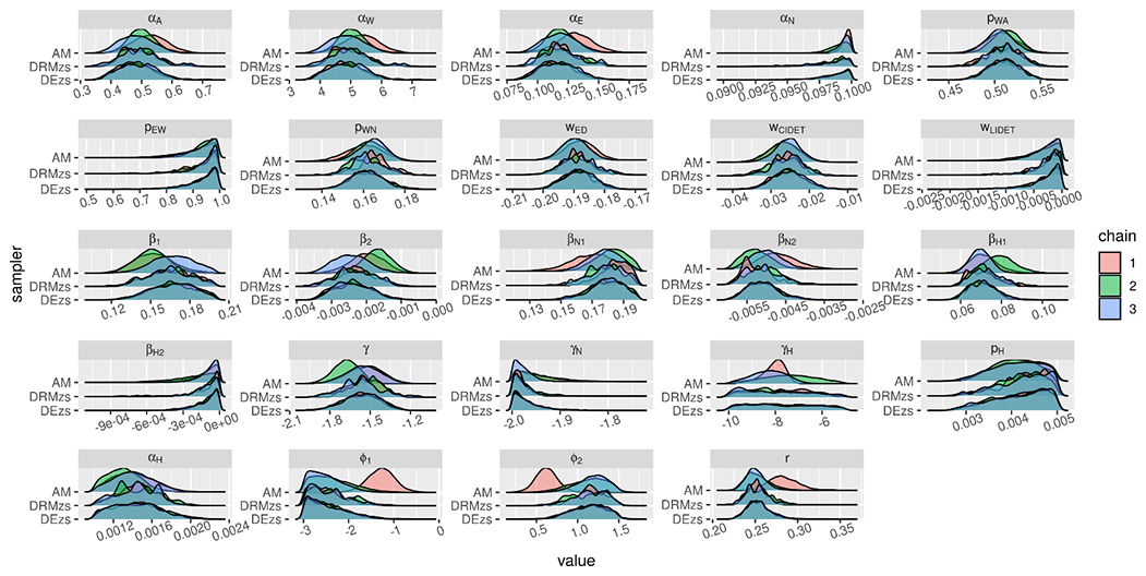
The first step was to determine if there is a notable difference in how the different calibration methods perform with the global dataset. All three calibration methods (AM, DEzs, DREAMzs) produced similar maximum a posteriori (MAP) values for global (joint) calibration when all data streams were used (Fig. 1, Table S4). Closer examination of different chains, though, shows that while DEzs and DREAMzs converged to the same parameters, individual AM chains instead produced different parameter distributions, and thus the calibration itself did not converge. The AM chain parameter distributions already settled into these distributions based on the initial parameter values given to them, and even after doubling the number of iterations (not shown) the distributions remained the same. In our view, this is indicative of what would happen if a simple single-chain calibration was done with SOC models. The Gelman–Rubin (G–R) statistics for the different calibration methods (Table S4) reflect these differences in convergence as well, with DEzs having the values within the acceptable boundary while values for AM are above acceptable ranges. DREAMzs also performs generally well but shows more divergence with the parameter values than DEzs. Similar behaviour was seen when running the individual dataset calibrations; individual AM chains would mix well but converged at different values from each other (not shown). Per global calibration diagnostics of different algorithms, we decided to report the rest of the results with the DEzs algorithm for clarity as its estimates converged best out of the three examined methods. When the global calibration with the DEzs algorithm was repeated with the Hobbie3 dataset included, the resulting parameter distributions were nearly identical to the calibration done without the Hobbie3 dataset included (not shown).

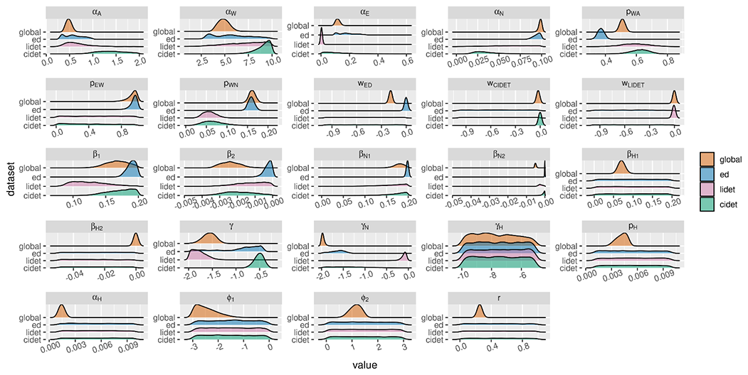
Figure 2 The estimated parameter distributions using DEzs with different calibration datasets.

3.2 Parameter estimates and correlations

The next step was to examine how the use of multiple datasets simultaneously affected the calibrated parameter sets compared to when using only individual datasets for calibration. The parameter sets produced by the calibrations differ from each other to a meaningful degree in both the parameter mean value and the associated uncertainty range (Fig. 2; Table S5). Despite that, though, there are certain patterns in the parameter sets: the pool decomposition rate relationships remain the same in that W has the quickest turnover rate followed by A, with N being the slowest to decompose. With the climate terms, both CIDET and LIDET calibrations have difficulties in settling on the climate terms while covering a multitude of different climate types, while ED calibration, whereby the climate differences between measurement locations are minor, produces a relative narrow climate parameter estimate. The global calibration, however, does clearly converge around certain climate parameters even if the uncertainty range remains wide. And even though the ED dataset has the most detail about the AWEN distribution, the AWE decomposition rates estimated based on it do not appear to converge, with multiple peaks in the parameter distributions.

Figure 3 Parameter correlations for the global calibration with the DEzs algorithm.

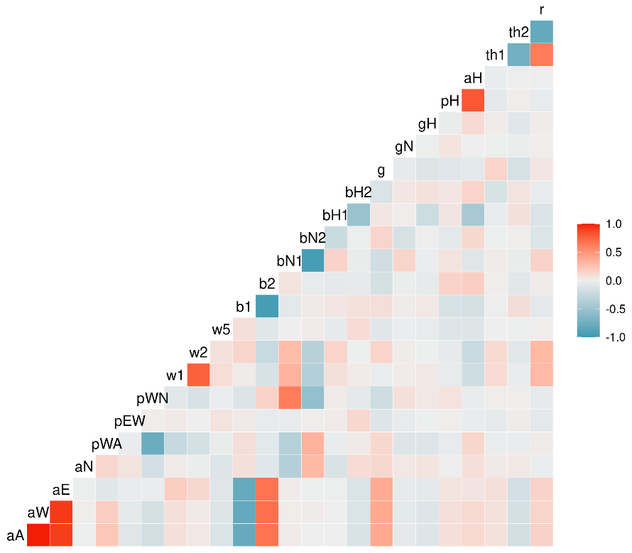
To further examine the parameter calibration, we analysed the correlations between different parameter values produced by the DEzs algorithm from the global calibration (Fig. 3), which shows that the correlations are the strongest between processes affecting the same pools. The p terms, which had been set to 0 and 1, were excluded from the correlation analysis since they did not vary during the calibration. The AWE pool decomposition rates have strong positive correlations between the decomposition rates and with the climate driver terms affecting decomposition in them. Similarly, there is strong negative correlation between the temperature terms affecting the same pools and a strong positive correlation between the H pool terms. There are both strong positive and negative correlations with the size-related parameters. While the exact correlation values changed depending on the calibration dataset, the general relationships remained similar (not shown).

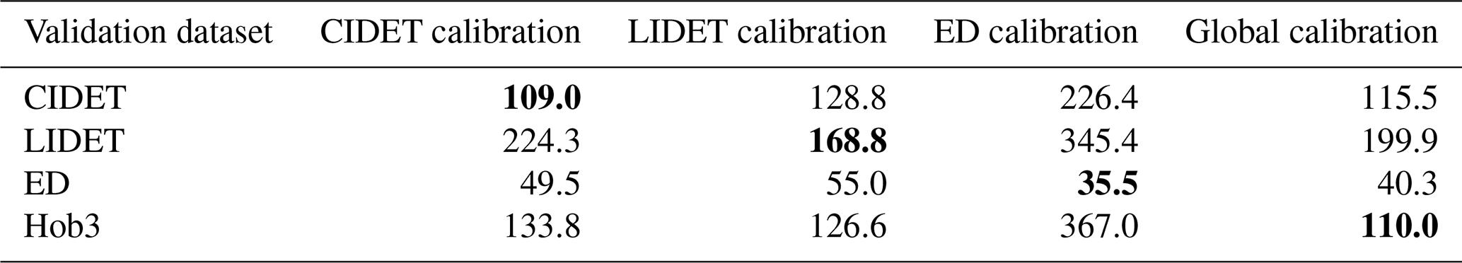
Table 3 The RMSE values for the different validation datasets when the model is run with the MAP values from the calibrations done with the different datasets. As with the measurements, the RMSE unit here is grams. The lowest RMSE for a particular dataset is bolded.

3.3 Validation and comparison to Yasso07

The final step was to validate how the different parameter sets perform with separate validation datasets and determine if there are notable systematic errors with regard to the climate driver data. For each dataset, the RMSE values are at their lowest when using the parameter sets calibrated with that specific dataset (Table 3), though the global parameter set produced RMSE values close to those lowest values. However, when using the parameter sets calibrated by datasets other than that one the validation data have been chosen from, the RMSE values became higher, indicating worse model performance. When the RMSE analysis was done with the Hobbie3 dataset, the global parameter showed the best performance. It should be noted that since in the ED dataset measurements are for each individual AWEN pool, the individual measurements are smaller in value than the total mass measurements of CIDET, LIDET, and HOB3. Consequently, the RMSE values for ED are smaller than those for CIDET, LIDET, and HOB3 datasets.

Table 4 Averaged measured SOC and projected SOC values with both Yasso07 and Yasso20 for forest plots in Hyytiälä, Finland, classified by measurement site (units: kg C m⁻²).

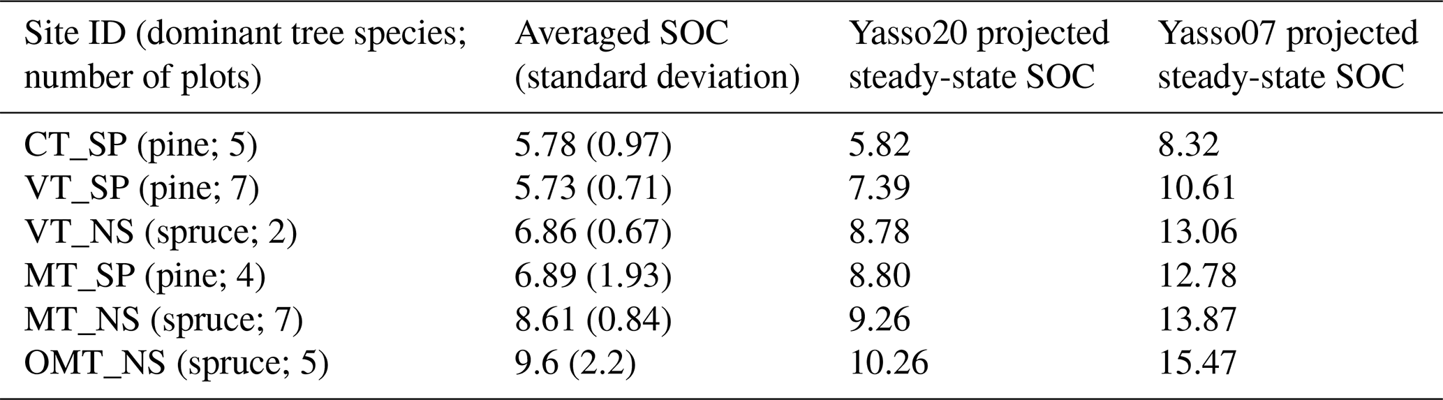
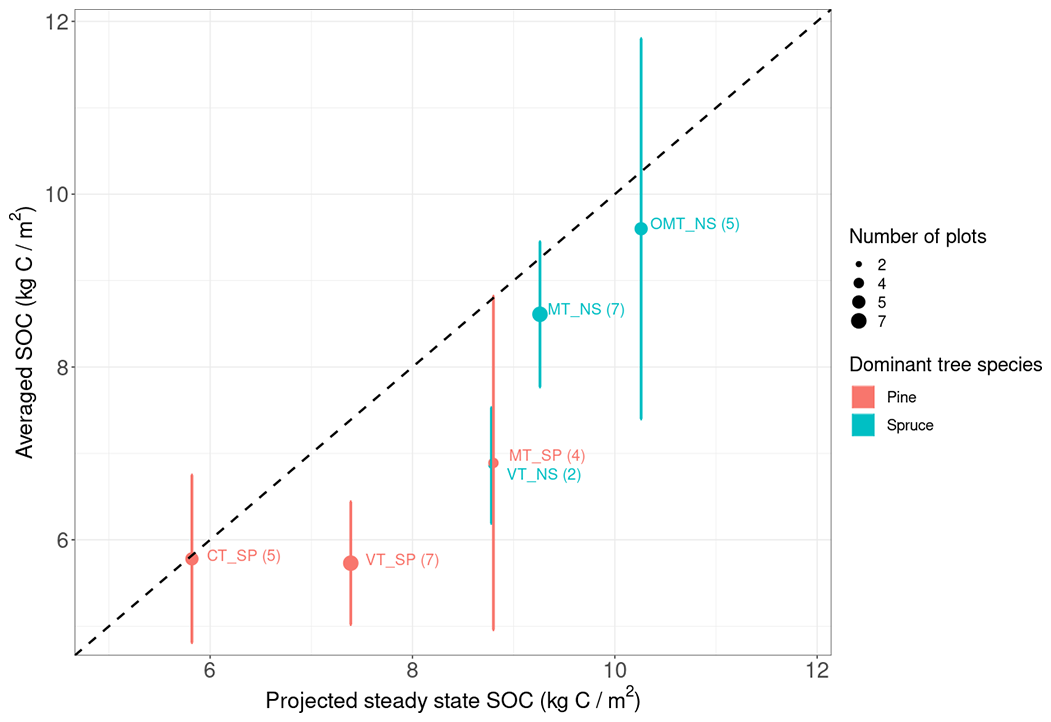
Figure 4 The projected steady-state SOC compared to the averaged measured SOC values in plots from multiple measurement sites.

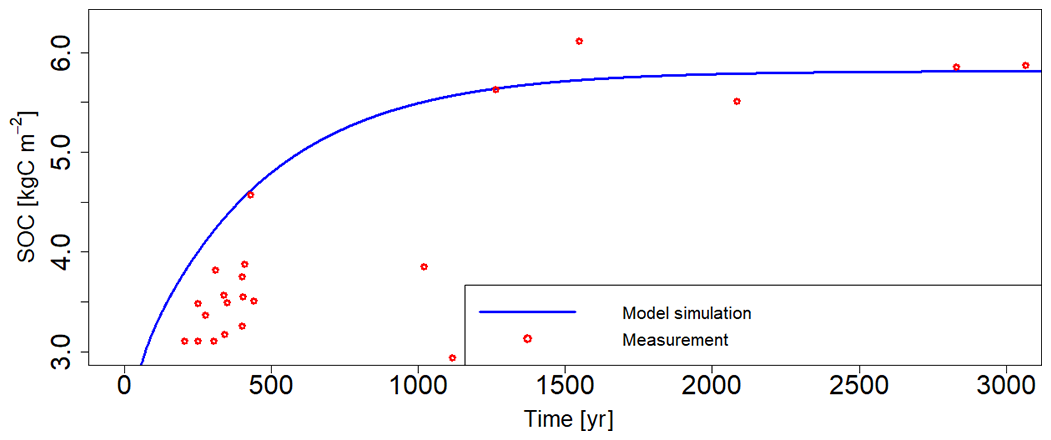
Figure 5 Measurement-based (red dots) and model-based (blue line) projections of SOC accumulation on the Finnish coast after the end of the ice age.

With regard to the long-term SOC projections, the comparisons with the Hyytiälä forest plot measurements (Table 4; Fig. 4) indicate that at least in the Nordic forests Yasso20 potentially slightly overestimates the steady-state SOC, with the largest differences still being below 2 kg C m⁻². It should be noted, though, that there is notable variance within the measurements in addition to the uncertainty related to the driver data. The chronosequence data (Fig. 5) show that the model projection saturates in approximately 1000 years, similarly to the measurements.

When examining how Yasso20 performs relative to Yasso07, the RMSE for Yasso07 projections is 118.2 g compared to the Yasso20 RMSE of 110 g. With the Hyytiälä forest plot measurements (Table 4), in all plots Yasso07 overestimated the SOC by at least 3 kg C m⁻² more than Yasso20. However, when examining the distribution of carbon into different pools in these steady states (not shown), more meaningful differences were revealed. For Yasso07, only ∼37 % of the SOC was in the long-lived H pool, while ∼50 % of the carbon was in the N pool. By comparison, with Yasso20 projections ∼54 % of the carbon is in the long-lived H pool and ∼27 % in the N pool.

Figure 6 The remaining decomposing carbon for a hypothetical straw litter in Hyytiälä, Finland, climate conditions when simulated with Yasso07 (solid red) and Yasso20 (dashed blue) with a (a) 20-year and (b) 100-year time window.

The hypothetical straw litter decomposition (Fig. 6) shows that while the total carbon remainder amounts for the two models are close to each other for the first 10 years, after that there is a clear divergence between the model projections, with Yasso07 having more remaining carbon than Yasso20. More detailed inspection of the results (not shown) found that this difference was due to the N pool decomposing at a much slower rate than in Yasso07 than in Yasso20. This also causes less carbon to accumulate in the H pool in Yasso07 than in Yasso20, with the latter having approximately twice as much carbon in the H pool than the former after 50 years. When repeated with warmer climate drivers (not shown), the Yasso07 time series projection decreases at a faster rate than the Yasso20 time series projection.

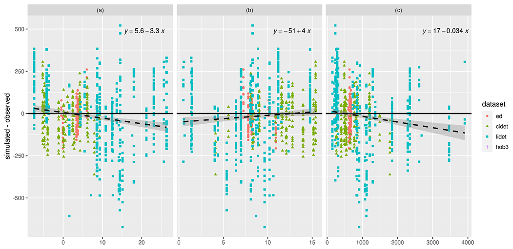
Figure 7 Residual analysis between simulated and observed carbon remnant on (a) mean temperature (^∘C), (b) temperature variation (^∘C), and (c) total precipitation (mm yr⁻¹) at the validation site.

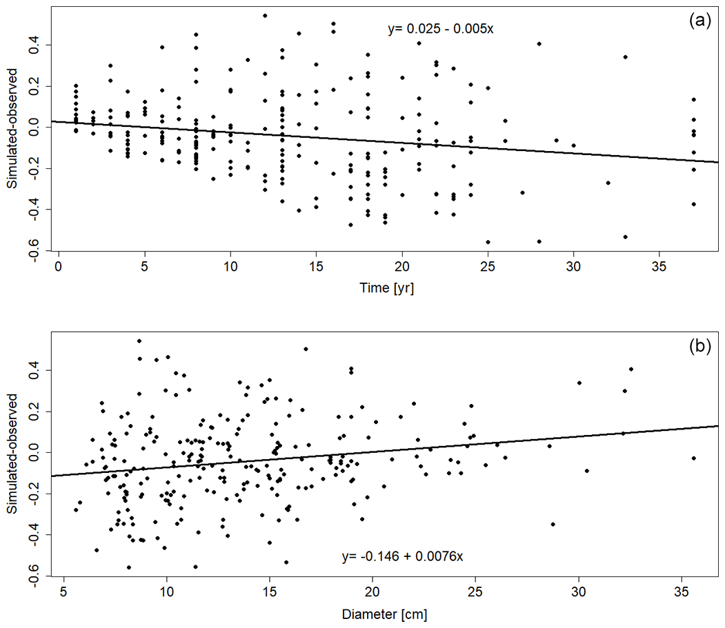
Figure 8 Residual analysis between simulated and observed carbon remnants of wood decomposition from Mäkinen et al. (2006) on (a) decomposition time and (b) diameter.

3.4 Residual analysis

When checking residuals from the litter-bag experiments against mean annual temperature, annual temperature variation, and total annual precipitation (Fig. 7), there appears to be a tendency for Yasso20 to increasingly underestimate the remaining litter-bag C with growing average mean temperature and precipitation. The error does not, though, show any signal when looking at the temperature variation within the year. With the woody decomposition residuals (Fig. 8), there is a slight negative trend over time and a slight positive trend over size. Both are minor, though, and the residuals for the woody decomposition are relatively evenly distributed for the validation dataset.

4 Discussion

4.1 The benefit of calibrating with multiple datasets

Our results show that simultaneously using multiple datasets from different environments improves the general applicability of the SOC model even when the simplistic leaching factor approach had to be used to be able to compare different litter-bag datasets and detailed uncertainty estimates were lacking, confirming our first hypothesis. This is in line with prior studies arguing for larger representation in the calibration data (Zhang et al., 2020). Furthermore, a more detailed analysis of different calibrations shows (Fig. 2) that the information from multiple datasets is in truth even necessary for the calibration, as when calibrating only with one dataset, the decomposition parameter uncertainty ranges were either large or, in the case of the more nuanced EURODECO dataset, did not even appear to converge. Something that was not examined in this study was how the uncertainties for the different datasets should be defined. Even if the assigned measurement uncertainties were correct for each dataset, combining them introduces structural uncertainties that should also be accounted for (MacBean et al., 2016). A potential method to address this would be to estimate the dataset uncertainties along with the model parameters, as done, for example, in Cailleret et al. (2020), but applying this approach to the SOC system will require a more thorough analysis in order to assess how it impacts the results.

Further inclusion of smaller dataset

Even with this global calibration, individual locations can be affected by specific SOC decomposition conditions not currently accounted for in models (Malhotra et al., 2019). Naturally, if smaller datasets of SOC and decomposition measurements are available from locations affected by specific decomposition dynamics, for example agricultural soils that are treated in a very specific manner, it would be logical to use that local information to constrain the SOC model to better suit that location. However, the results here raise questions on how those smaller datasets should be implemented in the model calibration. The inclusion of the Hobbie3 dataset did not meaningfully impact the calibration results (not shown), which is reasonable considering how small that litter-bag dataset (N=192) is compared to the totality of the other datasets ($N=\sim \mathrm{17}\mathrm{000}$ of which $N_{\mathrm{litter}\mathrm{bag}}=\sim \mathrm{12}\mathrm{000}$) used in the calibration. This indicates that due to the sheer size of the global calibration dataset, smaller local datasets cannot effectively be used just by adding them to the joint calibration process. Additionally, while the smaller datasets such as the Hobbie3 dataset contain site-specific information, they are measurements similar to the ones within CIDET and LIDET, and thus there is no reason to believe they would provide additional insight into the global application. There are other options, though, by either using the globally estimated parameter ranges as the priors for a calibration with the local data, re-weighing the different datasets based on expert opinion (Oberpriller et al., 2021), or employing a hierarchical calibration approach (Tian et al., 2020; Fer et al., 2021), but the impact of these approaches should be separately researched and tested. Our study still successfully provided a global parameter set that increases the applicability of the Yasso model and informs global SOC estimates.

4.2 Calibration method

Here we showed that by using a DEzs calibration algorithm, we were able to simultaneously use multiple different types of datasets to constrain the soil organic carbon (SOC) model Yasso and produce a converging parameter set. Additionally, using a more conventional model calibration approach, here the adaptive Metropolis (AM), showed that it was vulnerable to the local likelihood maxima and that the resulting parameter sets were strongly affected by the starting values. This supports our second hypothesis that more advanced calibration methods are necessary to better explore the likelihood surface and estimate SOC model parameters due to the trade-offs between the parameter values that result in equifinality in the parameter space. Furthermore, even the more stable calibration method produced different results for different individual datasets used to calibrate. More advanced calibration methods, though, then need to be applied to minimize the impact of the resulting uneven parameter space and produce Gelman–Rubin values within more acceptable ranges (Gelman and Rubin, 1992). Something that was curious in our results was that DEzs converged better than DREAMzs (Table S4) despite the latter being a more state-of-the-art method (Vrugt, 2016). We were not able to specifically determine the reason for this in our tests here; was it something related to the behaviour of the parameter space or to some aspect of the technical implementation?

4.3 Impact of prior parameter information

One of the fundamental challenges for calibrating SOC models is lack of experimental information regarding the model parameter value distributions. Therefore, we used generally broad uniform prior distributions for the calibration here. However, it is still important to evaluate the calibration results based on our understanding of the overall system behaviour. For example, initially we used wider priors for parameters p_H and α_H (results not shown), which in turn resulted in the calibration producing a p_H value of ∼0.08 and, consequently, a much higher H pool decomposition rate. As this did not fit the system behaviour seen, i.e. with the bare fallow experiments (Menichetti et al., 2019) or the soil chronosequence (Fig. 3), we applied a narrower prior constraint on the related parameters. Another, and a more complicated, example is that when using wider prior constraints for the N pool decomposition rate parameter α_N, the calibration resulted in the N pool being largely insensitive to the temperature and moisture drivers. While there are no direct measurements of the lignin pool temperature sensitivity, there have been studies showing that the energy needed for breaking down SOC compounds increased with complexity (Davidson and Janssens, 2006; Karhu et al., 2010), indicating that the N pool should be temperature-sensitive. Here we chose to constrain α_N to a lower range, which in turn forced a climate driver sensitivity for it. All these examples illustrate that prior information and expert opinion should directly inform the calibration, and the calibration results themselves should be further reassessed in their physical meaning.

4.4 How Yasso20 performs in comparison to Yasso07

When comparing the litter-bag validation dataset performances of Yasso07 and Yasso20, there is an improvement with Yasso20 even though both models have been calibrated largely with the same litter-bag data. This underlines the fact that the added model detail and reconsidered calibration process have a positive impact on the model projections. What is more striking, though, is that Yasso20 did perform better across the board with the Hyytiälä SOC data than Yasso07 when the latter model's long-term SOC component was calibrated with Finnish conditions. This result argues that while local calibration data are important, even for those specific locations there could be a benefit in including global data in the calibration. These results validate the third hypothesis concerning the impact of the presented improvements on model performance.

A more thorough analysis of the model projections revealed a more fundamental difference in the model dynamics than initially indicated by the comparison datasets. In Yasso07 the N pool decomposes much slower, which impacts the rest of the decomposition dynamics and causes less long-lived H pool carbon to be formed during the soil decomposition. As a consequence of differences in the calibration procedures and the resulting model versions, Yasso07 projects higher SOC values than Yasso20 with the same input values, and these model versions would also react differently to changes in climate conditions and litter input.

The Yasso07 dynamics are most likely due to a combination of multiple factors, which highlights the complicated process of SOC model calibration. As Yasso07 was calibrated in segments, the woody decomposition parameters were calibrated after the AWEN H pool parameters were determined from the global litter-bag experiments and Finnish SOC measurements. When looking at the calibration results from individual datasets (Fig. 2) there are parameter sets there which have similarly low decomposition rates for the N pool as Yasso07. Depending on how the different measurement datasets were weighed, it might be that those datasets that favoured slower N pool decomposition had more impact than with Yasso20 calibration. Finally, in Yasso20 the climate driver parameters are different between the AWE and N pools, and while the temperature terms are close to each other, the precipitation terms do differ from each other, while in Yasso07 they would be the same. This would affect the Yasso07 dynamics during calibration. The calibration is made even more vulnerable to all these factors because a vast majority of the litter-bag data used here are from the first 6 years of decomposition during which Yasso07 and Yasso20 are very close to each with regard to total carbon remaining (Fig. 6). In such a situation it is very possible that less-developed calibration protocols can lead to unrealistic system dynamics that still appear to produce good results within limited time windows.

4.5 Leaching

As established in Sect. 2.2, in order to compare the measurements from different litter-bag experiments, there needs to be a parameter that accounts for the litter-bag type's impact on the mass loss rate (Tuomi et al., 2009). When testing with independent litter-bag data, we see that even with this added assumption, the global calibration produces a better fit than the calibration based on individual litter-bag campaigns (Table 3). This supports using data from multiple litter-bag campaigns in model calibration. However, in the results it is evident that not only are the leaching parameters estimated to be essentially zero when calibrating only with individual decomposition bag datasets (Table S5), but also when simultaneously calibrating with all the datasets, only the ED dataset ends up having a meaningfully non-zero value. First of all, this indicates that the current straightforward formulation for leaching is insufficient; as with the individual dataset calibrations, the other parameter values are able to produce fits where there is no leaching despite knowledge that it is a factor. Second, even when calibrating multiple datasets simultaneously, the calibration appears to apply the leaching effect to only one of the datasets even when it should affect all of them.

A further complication is that the differences in RMSE results (Table 3) suggest that there are systematic differences between the datasets resulting from various sources such as the experimental setup or environmental differences. As a consequence, calibrating with these kinds of datasets will result in systematic differences in model performance as established in Oberpriller et al. (2021) and as can be seen in how CIDET- and LIDET-calibrated Yasso performs with the ED dataset and vice versa. By being a corrective term, the leaching factor introduced here will also reflect all those other elements causing the systematic differences, for example different mycorrhizal environments, instead of just being about the physical properties of the litter bag. Due to all these factors, the leaching impact needs to be further studied and the relevant equations need to first be formulated with experimental data specifically gathered for that purpose. There also needs to be additional work in trying to better quantify what those other systematic error elements are so that they can be better addressed.

4.6 Humus formation and the need for the layer Yasso

There is an important point concerning the parameterized humus (H) formation term p_H here. The long-term H formation can only take place in the soil itself as it requires the presence of mineral compounds (Schmidt et al., 2011), which is why only the global soil carbon dataset in this study could be used to constrain H parameters. However, they are only point measurements with no information on how the state changes over time. Therefore, we have to assume that the measurements represent the approximated steady state from an assumed litterfall. This not only causes larger parameter uncertainties, but the estimated p_H parameter value will also represent the fraction of the total litterfall that ends up in the H pool, while in reality with the surface vegetation litter there needs to be an additional mechanism that transfers the carbon compounds to soil while root litter is already in that environment. Consequently, if examining litter decomposition taking place only in the soil, such as with roots, it is likely that p_H for that soil system would be larger than what is estimated here. This would fit previous research suggesting that the root biomass specifically appears to be connected to the amount of long-term carbon in the soil as more of it would be able to form H compounds than the surface vegetation (Clemmensen et al., 2013; Jackson et al., 2017). However, currently the amount of data that would allow efficiently separating the above- and below-soil decomposition processes during the calibration process is limited. Additionally, beyond this, there is the presence of mineral compounds and other conditions that affect how efficiently H is formed that should be included when formalizing H formation (Rasmussen et al., 2018). Better addressing the formation of H is a crucial development step for the model, but the current approach provides an initial way to estimate the H pool size and quantity.

4.7 Temperature and precipitation impact

At first glance it appears that the current version of Yasso20 overestimates SOC decomposition (i.e. underestimates SOC amount) at higher precipitation and temperature values, as indicated by the negative trend in Fig. 7. In the current formulation of environmental drivers (Eq. 5), only the lower precipitation values decrease the decomposition rate, with the system becoming insensitive to increases in precipitation after a certain threshold. However, it is known that at higher moisture levels the SOC decomposition rates decrease (Keiluweit et al., 2017). A more informative driver of moisture conditions (e.g. monthly soil moisture) and a more realistic response function could help disentangle the reasons behind this trend in the residuals in the future. The current version of Yasso20 uses precipitation as the driver instead of soil moisture because the decomposition bags from the datasets used as constraints here are on the surface and were thus expected to be primarily controlled by precipitation. In light of current findings, further steps in Yasso model development towards using soil moisture as model drivers are planned.

Closer examination of the error distribution over the climate drivers, though, suggests some more complexity. Even at the lower precipitation values, while both CIDET and ED data errors cluster approximately equally around zero, the LIDET data points show a shift towards negative errors, similarly to at higher precipitation values. Thus, it appears that the issue is at least partially due to the dataset itself rather than the pure precipitation signal. Similar behaviour can be seen with mean temperature, although it is not as pronounced. Thus, there is seemingly a systematic error when simulating the LIDET data with the global calibration parameter sets. It is unclear if this is due to something with the measurements, something with the processes, or if the climate driver data are not similarly representative of the conditions as with the other datasets used.

4.8 Litter size impact on decomposition

In the current Yasso20 implementation, the woody litter diameter does not change during the decomposition process, while in reality the wood shrinks as it decomposes. This explains why when comparing the model results to the tree decomposition validation dataset (Fig. 8), the model overestimates the decomposition rate for decades-old tree stems with a measured diameter of approximately 10 cm. In those cases, the model assumes that was the size of the trunks when the decomposition started and, consequently, the size impact is smaller than it should be. While the model still performs well with the validation database regardless of this, it is an important aspect to consider when applying the Yasso20 model with woody decomposition.

5 Conclusions

Soil organic carbon (SOC) models should be constrained by data from multiple different ecosystems reflecting the various dynamics affecting the SOC decomposition process. Using data from multiple datasets produced parameter sets which performed better in a global comparison than parameter sets calibrated with information from individual datasets, highlighting the necessity of using more data. However, the traditional AM calibration method had difficulties converging to a single parameter set when used with multiple datasets, most likely due to the numerous local likelihood maxima within the likelihood space, and our deliberate choice for avoiding detailed algorithm-specific configurations, which reduces repeatability and re-applicability. Consequently, our results showed that more advanced methods such as DEzs should be used when calibrating SOC models. Furthermore, we identified numerous aspects for which further detailed data are needed to better constrain the model processes in question, for example regarding the leaching parameter that allows comparison of different litter decomposition bag experiments or better connecting varying soil moisture conditions to changes in SOC.