the Creative Commons Attribution 4.0 License.
the Creative Commons Attribution 4.0 License.
 | 11 Jan 2022
Modeling reservoir surface temperatures for regional and global climate models: a multi-model study on the inflow and level variation effects
Yurii Shevchuk
Georgiy Kirillin
Pedro M. M. Soares
Rita M. Cardoso
José P. Matos
Ricardo M. Rebelo
António C. Rodrigues
Pedro S. Coelho
The complexity of the state-of-the-art climate models requires high computational resources and imposes rather simplified parameterization of inland waters. The effect of lakes and reservoirs on the local and regional climate is commonly parameterized in regional or global climate modeling as a function of surface water temperature estimated by atmosphere-coupled one-dimensional lake models. The latter typically neglect one of the major transport mechanisms specific to artificial reservoirs: heat and mass advection due to inflows and outflows. Incorporation of these essentially two-dimensional processes into lake parameterizations requires a trade-off between computational efficiency and physical soundness, which is addressed in this study. We evaluated the performance of the two most used lake parameterization schemes and a machine-learning approach on high-resolution historical water temperature records from 24 reservoirs. Simulations were also performed at both variable and constant water level to explore the thermal structure differences between lakes and reservoirs. Our results highlight the need to include anthropogenic inflow and outflow controls in regional and global climate models. Our findings also highlight the efficiency of the machine-learning approach, which may overperform process-based physical models in both accuracy and computational requirements if applied to reservoirs with long-term observations available. Overall, results suggest that the combined use of process-based physical models and machine-learning models will considerably improve the modeling of air–lake heat and moisture fluxes. A relationship between mean water retention times and the importance of inflows and outflows is established: reservoirs with a retention time shorter than ∼ 100 d, if simulated without inflow and outflow effects, tend to exhibit a statistically significant deviation in the computed surface temperatures regardless of their morphological characteristics.
- Article
(4010 KB) - Full-text XML
- Companion paper
- BibTeX
- EndNote


Numerical weather prediction (NWP) and climate modeling are essential tools in research and applied science applications (e.g., Bauer et al., 2015; Forster, 2017; Jacob et al., 2020). Motivated by the need to increase the reliability of climate and weather projections, the core numerical models undergo continuous improvements aiming at the best compromise between model representativity and computational efficiency (Flato et al., 2013). Air–lake heat and moisture fluxes affect the near-surface atmospheric layers and are essential to accurate estimation of the future climate or weather forecast. Therefore, parameterization of inland waterbodies in atmospheric modeling has quickly evolved to increase the accuracy of the land–atmosphere boundary layers (Bennington, 2014; Xue et al., 2017; F. Wang et al., 2019). According to previous studies, the presence of waterbodies significantly affects the turbulent heat exchange with the atmosphere (Philips, 1972; Bates et al., 1993; Niziol et al., 1995; Lofgren, 2006; Notaro et al., 2013; Wright et al., 2013). In northern latitudes, surface waters tend to absorb heat in summer and release it in autumn, damping the temperature fluctuations in their vicinity and creating a lag in both diurnal and annual cycles of the air temperature, as well as increased precipitation (Dutra et al., 2010; Nordbo et al., 2011; Samuelsson et al., 2010; Subin et al., 2012). Overall, missing the lake and reservoir effects has been shown to deteriorate the results of regional and global climate simulations (Ljungemyr et al., 1996; Long et al., 2007; Deng et al., 2013; Dutra et al., 2010; Samuelsson et al., 2010; Subin et al., 2012; Le Moigne et al., 2016; Irambona et al., 2018).
Waterbodies display larger thermal inertia than the surrounding land areas due to the high specific heat capacity of water and the vertical turbulent heat transport from the water surface to its deeper layers. Furthermore, they absorb a higher fraction of solar radiation than land due to a lower albedo and a higher transparency. The heat storage and thermal characteristics of inland waterbodies, acting primarily but not only through water column stability, are influenced by bathymetry, surface area, turbidity, and ice conditions (Schertzer, 1997; Rouse et al., 2003; Oswald and Rouse, 2004; Magee and Wu, 2017). Surface heat fluxes, in particular the evaporation rate, are also affected by advection due to inflows and outflows (e.g., deepwater withdrawal) and by water level (WL) fluctuations (Rimmer et al., 2011; Friedrich et al., 2018). These fluctuations are usually much more pronounced in reservoirs than in natural lakes. Herewith, neglecting the aforementioned water budget variations may lead to errors in surface heat flux predictions, especially in reservoirs.
The progressive increase in the spatial resolution of general circulation models (GCMs) and regional climate models (RCMs) resulted in wide implementation of coupled one-dimensional (1-D) models simulating surface energy fluxes in waterbodies, neglecting, however, the variation of inflows, outflows, and WL. The coupled lake and reservoir models differ among each other mainly by the vertical mixing parameterization, classified into three major categories: eddy diffusion models, turbulence models, and bulk mixed layer models. In eddy diffusion models, vertical turbulent mixing is defined by eddy diffusion parameterized as a function of velocity and stratification strength in the form of the gradient Richardson number (e.g., HOSTETLER model, Hostetler and Bartlein, 1990; SEEMOD, Zamboni et al., 1992; LIMNMOD, Karagounis et al., 1993; MINLAKE, Fang and Stefan, 1996; CLM, Oleson et al., 2004; CLM4-LISSS, Subin et al., 2012; WRF-Lake, Gu et al., 2015). More complex approaches, based on the k−ε turbulence model, parameterize eddy diffusion based on the Kolmogorov–Prandtl relationship (Svensson, 1978; Burchard et al., 1999; Goudsmit et al., 2002; Stepanenko and Lykossov, 2005). Bulk mixed layer models rely on the self-similarity concept for the temperature–depth profile in the stratified layer and integral budgets for the mixed and bottom layers (Kraus and Turner, 1967; Mironov et al., 2010). The performance of some of these models has already been evaluated in modeling intercomparison studies (e.g., Perroud, 2009; Stepanenko et al., 2010, 2013; Thiery et al., 2016; Huang et al., 2019; Y. Wang et al., 2019; Guseva et al., 2020). Generally, these intercomparison studies evaluated the model performance with application to one to three lakes, usually with very particular morphological characteristics (e.g., very deep or very shallow), over a limited time period. Overall, the results of these studies had an important impact on the further development of the models. In particular, they highlighted the need for intercomparison research projects that include a larger number of waterbodies and a longer modeling simulation.
Data-driven models such as artificial neural networks (ANNs) have not yet been considered for the parameterization of lakes in climate models. Nevertheless, they have been successfully used to estimate mean daily and hourly water temperatures in rivers (e.g., Chenard and Caissie, 2008; Hebert et al., 2014) and in lakes (Sharma et al., 2008; Samadianfard et al., 2016; Read et al., 2019). The approach is particularly advantageous when the modeled processes are complex and nonlinear (Sharma et al., 2008), as in the case of surface water temperature (SWT). In view of the trade-off between results quality and computational efficiency, data-driven models have potential advantages in estimating the effect of lake inflows and outflows on SWT, which motivates their inclusion in model intercomparison studies.
Currently, the major challenge in the parameterization of lakes and reservoirs in climate models is the need to ensure that the models' response is consistent and accurate considering the wide range of morphological characteristics and the high variability of the meteorological forcing. While incorporation of inflows and outflows may crucially improve the quality of model predictions, the increased complexity can restrain extension of process-based models and require alternative data-based approaches.
In this study, we evaluate the importance of the energy transfers due to water inflows and outflows when modeling surface water energy fluxes in artificial reservoirs and elaborate a methodology to improve this essential aspect of RCMs and GCMs. For this purpose, we (i) model 24 Portuguese reservoirs by using four models. These are a 2-D model to define a calibrated and validated baseline scenario, two 1-D models without the parameterization of inflows or outflows, and an ANN to (ii) assess the modeling error in SWT of lakes (similar to a seepage lake) and reservoirs potentially associated with atmosphere–lake interactions and (iii) compare the performance and computational requirements of different approaches to predict the evolution of SWT in lakes (similar to a seepage lake) and reservoirs.

Figure 1Location of the simulated waterbodies (ordered according to the simulated mean volume from smallest to largest).
Portugal is located in southern Europe and has a typical Mediterranean climate. Maximum daily mean air temperature ranges from 13 ∘C in the central highlands to 25 ∘C in the southeast region. The minimum daily mean air temperature ranges from 5 ∘C in the northern and central regions to 18 ∘C in the south (Soares et al., 2012a). Complex topography and coastal processes define the spatial and temporal heterogeneity of precipitation, which differs from a relatively wet annual maximum above 2800 mm yr−1 in the mountainous northwest to a much drier 400 mm yr−1 in the tendentially flat southeast (Soares et al., 2012b; Cardoso et al., 2013).
The 24 reservoirs selected for this study are almost entirely located in mainland Portugal apart from Alto Lindoso (R19) and Alqueva (R24) reservoirs, which are shared with neighboring Spain (Fig. 1).
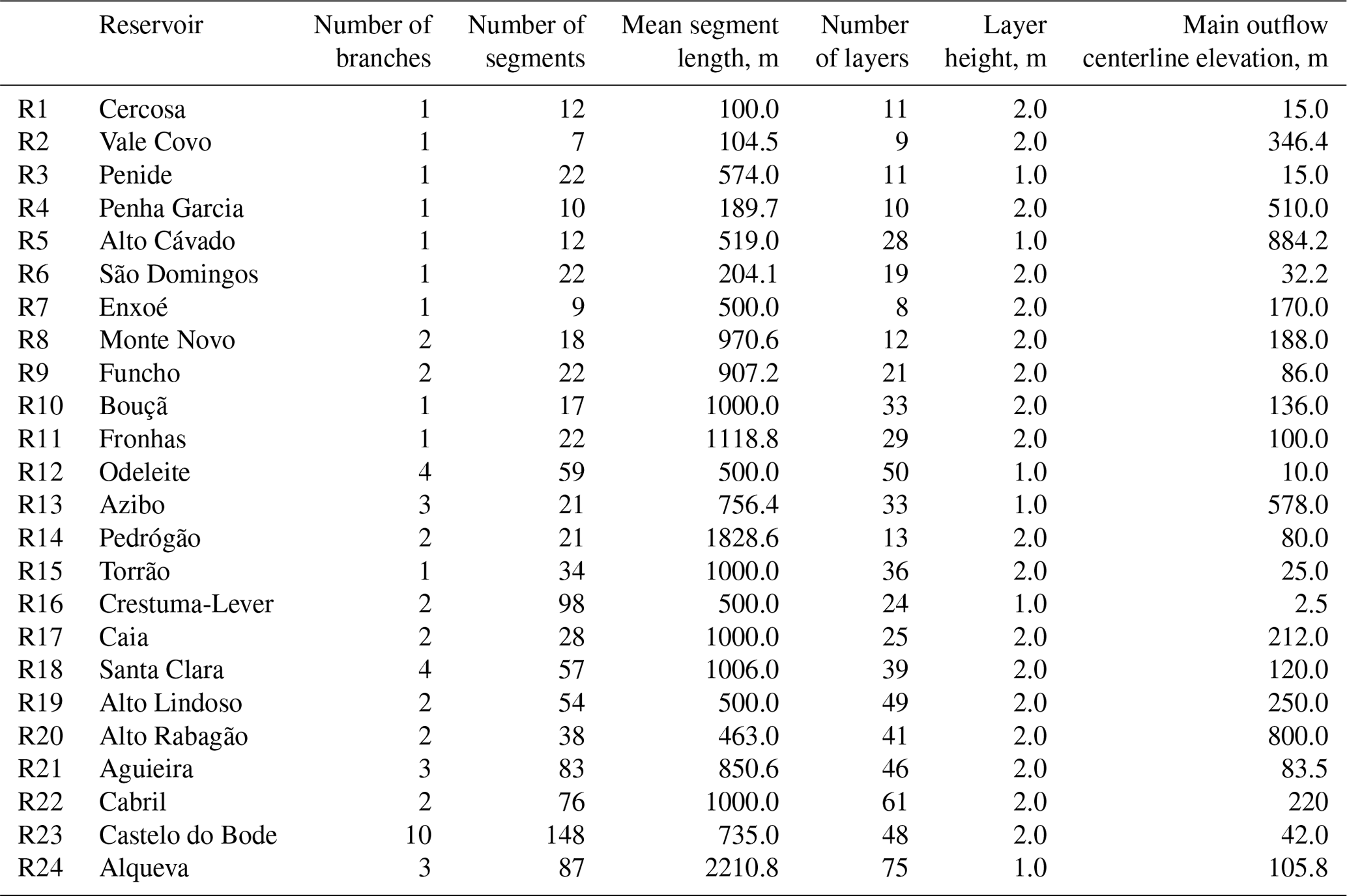
The reservoirs were selected for the study based on their water residence time (WRT) and morphological characteristics (volume, depth, surface area) (Table 1). Most of reservoirs are classified as warm monomictic, with a stratified period during the warmer months (May–September) and one mixing period each year during the colder part of the year from October to April. As exceptions, Cercosa (R1) and Torrão (R15) are weakly stratified, while Penide (R3), Penha Garcia (R4), Enxoé (R7), and Crestuma-Lever (R16) (a run-of-the-river hydropower scheme located in the north coastal region) are well mixed during the entire year.
Table 1Morphometric details of the reservoirs and main water uses.
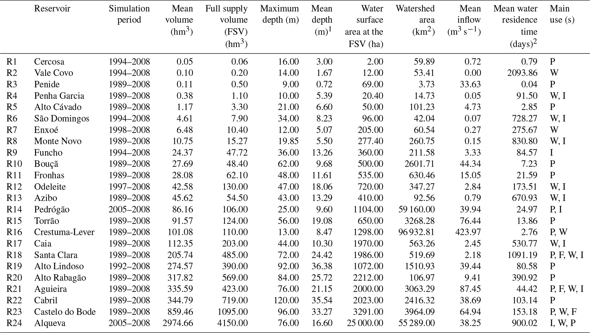
a P – power generation; W – water supply; I – irrigation; F – flood prevention. 1 The mean depth results from the division of the mean volume and the mean water surface area. 2 The mean water residence time is the ratio between the mean volume of the reservoir and the mean inflow.
3.1 Models and scenarios
To evaluate the importance of inflow and outflow in SWT simulations, a 2-D numeric model and two 1-D models were applied. Table 2 shows a full description of the scenarios considered in the development of this study.
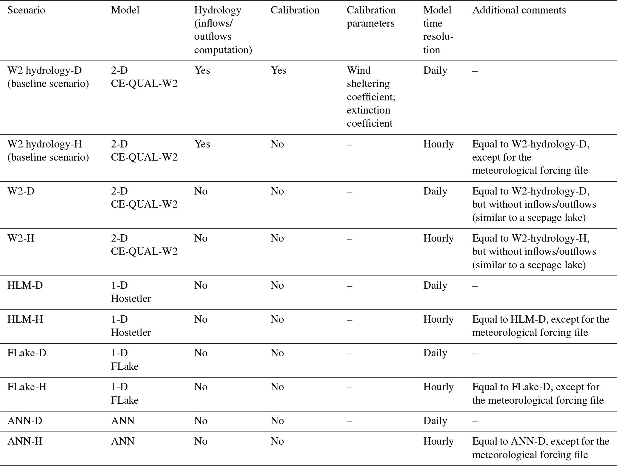
Since the model validation was limited by the scarcity of temperature profile measurements and observed time series of SWT, a major challenge of this study consisted of developing realistic baseline scenarios (forcing data and targets; W2 hydrology scenarios) having the necessary continuity and heterogeneity to evaluate the performance of different models. To overcome this limitation, a well-established 2-D model, CE-QUAL-W2 version 3.6 (Cole and Wells, 2008), was validated with observed data and used to create the baseline scenario forced with daily and hourly meteorological datasets covering a period of 20 years from 1989 to 2008 (with the exceptions described in Table 1). The 2-D model, forced with daily meteorology and monthly inflows and outflows, was calibrated by minimizing the mean absolute error (MAE) between simulated water temperature profiles and measurements spanning the period from 1989 to 2008 made in each reservoir, in all cases near the dam (W2 hydrology-D). After each model run, results were compared with the observed datasets and if needed the calibration parameters were retuned manually. The wind-sheltering coefficient (WSC) and the extinction coefficient for water were the only parameters modified at each model run. These parameters varied in the range from 0.1 to 1.0 and from 0.25 to 1.0, respectively. Data on the mean water extinction coefficient were available for four reservoirs: Bouçã (μ=0.27; σ= 0.05), Crestuma-Lever (μ=0.67; σ= 0.15) −0.67, Cabril (μ=0.27; σ= 0.05), and Castelo do Bode (μ=0.26; σ= 0.05); therefore, they were not calibrated. All 1-D simulations were performed with a constant water extinction coefficient value of 0.45, corresponding to the reference value suggested by Cole and Wells (2008). According to the eutrophication criteria defined by the OECD (1982), this value of water transparency is associated with eutrophic unstable systems and is also close to the mean value of 0.37 obtained from the four reservoirs listed above.
An alternative baseline scenario was produced by forcing the model with hourly meteorology (daily values were used for the first one), enabling evaluation of the sub-daily convection effects on the overall results. Daily and hourly baseline scenarios were designated “W2 hydrology-D” and “W2 hydrology-H”, respectively.
To assess the importance of heat transfer and mixing within the waterbodies, the two W2 hydrology scenarios were modified and simulated in a steady-state “constant mass budget” excluding precipitation, inflows, or outflows. These steady-state scenarios were designated “W2”. Apparently, W2 simulations maintain a constant water level corresponding to the full supply level (FSL). SWT time series, obtained with both scenarios W2 hydrology and W2, were compared using statistic error measures (see Sect. 3.3 for more details), assessing the relationship between the reservoir WRT and the error resulting from the neglect of advection due to inflows and outflows (as mentioned in the Introduction, a common feature of contemporary GCMs and RCMs).
The baseline scenarios (W2 hydrology) were defined to address the following questions.
- i.
How large is the uncertainty associated with the neglect of inflows and outflows?
- ii.
How adequate is the performance of simplified 1-D models compared with the state-of-the-art calibrated 2-D model, including parameterization of inflows and outflows as well as WL variation? What is the relative contribution to the final model error of the inflow and outflow neglect vs. neglect of the wind sheltering in meteorological forcing?
- iii.
Can we identify conceptual differences in representation of the fundamental physical processes (such as differences in the conceptualization of diurnal variations of SWT) by 1-D and 2-D models through the comparison of outputs from daily versus hourly forcing?
- iv.
How well can ANN simulate the evolution of a reservoir SWT?
The reliability of the baseline scenarios (W2 hydrology) for representation of the reservoir thermal regime has been demonstrated by the model calibration results and is supported by the outcomes of a large number of successful model applications worldwide (vide Cole and Wells, 2008). Using 2-D modeling results as a baseline “benchmark” scenario for validating 1-D models allows the isolation of the errors associated with the quality of meteorological forcing and observed data (e.g., water temperature datasets) while providing the continuity usually unavailable from observational datasets. Hence, the error obtained when comparing 1-D versus 2-D model results is to be regarded as an analytical variable encapsulating differences among the different scenarios and not the conventional model error (model output versus observed data).
While generally accurate, the use of calibrated 2-D models in the scope of complex GCMs and RCMs is restricted by high computational costs. Therefore, the next step of the analysis aimed at evaluation of more computationally effective 1-D models typically used to parameterize waterbodies within GCMs and RCMs. The reservoirs were simulated with a 1-D eddy diffusion model based on the approach considered by Hostetler and Bartlein (1990) and a 1-D bulk mixed layer model (FLake), both forced with hourly and daily meteorological data. Meteorological datasets considered in the modeling process included air temperature (∘C), relative humidity (%), wind velocity (m s−1), wind direction (rad), cloud fraction (0 to10), and shortwave solar radiation (W m−2). These datasets were considered in all models with the following exceptions: wind direction is not considered for 1-D model forcing, and the ANN modeling relies on the air temperature, relative humidity, and wind velocity datasets only.
The eddy diffusion model considers the vertical variation of both eddy diffusion and cross-sectional area. Simulations were undertaken using the maximum depth. In turn, FLake operates with volume-integrated equations. Accordingly, its simulations were performed based on the mean reservoir depth. Results obtained with the 1-D models, without any reservoir-specific calibration, were compared with the baseline scenarios obtained with the 2-D model (W2 hydrology). In addition to the 1-D models, SWT in all the reservoirs was modeled with an artificial neural network (ANN) trained using the momentum gradient-based optimization algorithm (Qian, 1999). SWTs from both daily and hourly 2-D baseline scenarios (W2 hydrology), covering the period from 1989 to 2004 and the predictor variables described in Table 3, were used to improve the input data dimension (Fig. 2).
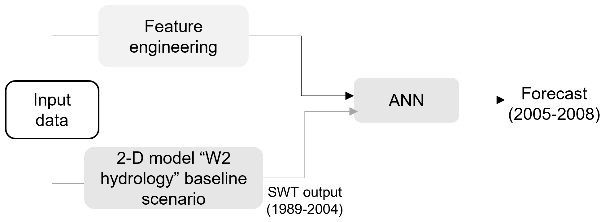
Table 3Predictor variables considered for the training and validation of the ANN.
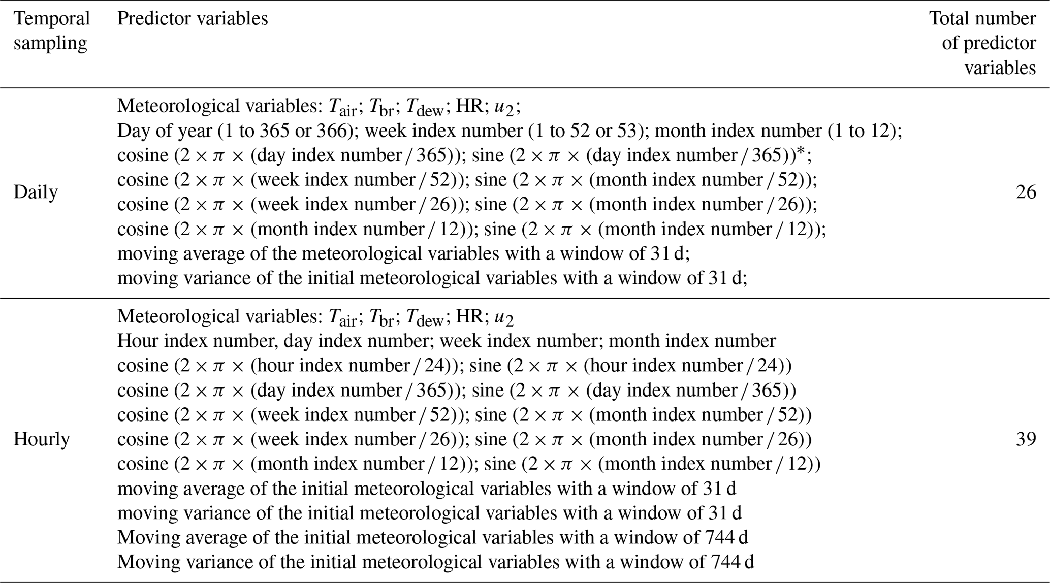
*Cosine and sine series reproduce cyclical yearly variations that can be recognized by the ANN in the inputs without any breaks (as is the case if linear series such as the day of year are used: large jump from 365 to 1 at the beginning of a new year).
Two different temporal resolutions of the input meteorological data, daily and hourly, were used to train and validate the ANNs; 80 % of the data was used for finding optimal network weights (of which 70 % was directly applied in the training and 30 % was employed in validation). This 80 % covered 16 years from 1989 to 2004. The daily discretization resulted in a dataset with N= 5843 entries, while the hourly discretization produced N= 140 232. The remaining 20 % of data had no intervention in the search for optimal network weights and covered the period from 2005 to 2008. This period, considered for the ANN forecast, included three dry years of 2005, 2007, and 2008 and one wet year, 2006. All the years were warm except for the cold year of 2008. The daily discretization resulted in a dataset with N= 1461 entries, while the hourly discretization produced N= 35 064. When the reservoir total simulation period (see Table 1) was shorter than 20 years, the dimension of the test dataset was preserved, and the training and validation datasets were reduced. The raw input data used to train the networks included the SWT obtained from the baseline scenarios prepared with the 2-D model, air temperature (Tair), inflow water temperature (Tbr), dew point temperature (Tdew), relative humidity (HR), and wind velocity (u2). In order to improve model performance additional time series were included as input. They were defined to provide implicit information about seasonal changes (Table 3).
The input time series were subsequently standardized through removal of the mean and scaling to unit variance. After the initial tests, which included different network architectures, backpropagation algorithms, regularization strategies, learning rate rules, activation functions, parameter initialization, and the extraction and transformation of features from the input meteorological data, the algorithm was selected whose results were in the best agreement with SWT from the baseline scenario simulated with the 2-D model (see Sect. 3.3 for more details). Beside accuracy, the computation time can also be a critical factor in the suitability of models to be used within GCMs or RCMs. The simplified 1-D models considered in this study have a clear advantage regarding the computation time when compared with more complex 1-D and 2-D approaches – a condition that was at the core of their development and that is directly linked with the neglect of inflows and outflows. Recognizing the importance of computational efficiency, the analysis included the quantification of the overall computation times for the process-based physical models and for the ANN. This evaluation was produced with a 2.21 GHz Quad-Core Intel Core i7 (memory: 16 GB 1600 MHz DDR3) by repeating each simulation 20 times.
3.1.1 2-D water quality and hydrodynamic modeling – CE-QUAL-W2
Due to the lateral and layer averaging of the governing equations, the 2-D hydrodynamic and water quality model CE-QUAL-W2 version 3.6 (Cole and Wells, 2008) is particularly suitable for modeling relatively long and narrow waterbodies, where transverse variations in velocities, temperatures, and constituents are negligible. Outlet geometry, outflows, and in-pool densities are the input to the selective withdrawal algorithm that calculates vertical withdrawal zone limits. Among the two model options of the withdrawal – line sinks, which are wide in relation to dam width (), and point sinks, which are narrow in relation to dam width () – only point sinks were considered. The point-sink approximation assumes the flow is radial both longitudinally and vertically (Cole and Wells, 2008). Therefore, for the outflow structure definition, the centerline elevation of the structure was included in the model (Table 4). Additionally, as suggested by Cole and Wells (2008), the algorithm was allowed to retrieve water from the top elevation of the computational grid. The model has been widely applied to stratified water surface systems such as lakes and reservoirs around the world, including Portugal (e.g., Diogo et al., 2008; Almeida et al., 2015). In order to illustrate the performance of CE-QUAL W2 in reservoir thermal simulations, Cole and Wells (2008) describe the calibration results obtained for 70 reservoirs. In their study, the MAE obtained for all reservoirs was smaller than 1.0 ∘C, and for many of them much smaller. The result can be considered outstanding, especially considering that errors were partially related to the quality of the boundary conditions and forcing meteorological data. The Ultimate algorithm was considered to be the solution for the numerical transport for temperature and constituents (Cole and Wells, 2008). Surface heat exchange was computed with the term-by-term algorithm described by Cole and Wells (2008). The reservoirs' bathymetry was defined from 1:25 000 topographic charts of the watersheds. Hence, each reservoir's computational grid is described by a specific number of branches, segments, and layers (Table 4).
3.1.2 Eddy diffusion model – Hostetler model (HLM)
The governing equation for the 1-D eddy diffusion model is based on Hostetler and Bartlein (1990):
where T, t, z, A, km, K, Cw, and Φ are water temperature (∘C), time (s), depth (m), area (m2), molecular diffusion ( m2 s−1), eddy diffusion (m2 s−1), the volumetric heat capacity of water (J m−3 ∘C−1), and a heat source term (W m−2), respectively. Within the model, eddy diffusion is computed at each depth with the analytical representation developed by Henderson-Sellers (1985) as a function of the 2 m wind velocity (u2) and a latitude-dependent parameter of the Ekman profile.
The surface boundary condition is described by the following equation.
The net surface heat flux (qn) (W m−2), which is the algebraic sum of solar radiation, atmospheric radiation, latent and sensible heat fluxes, and back radiation, was computed with the equilibrium temperature approach defined by Edinger et al. (1968), while latent and sensible heat fluxes were computed explicitly from surface water temperature with the same expressions defined in Cole and Wells (2008). In this study the heat transferred from the sediments to the water column has been neglected. Accordingly, the bottom boundary condition takes the following form.
The solution of the heat diffusion equation was obtained by resorting to the implicit numeric Crank–Nicolson scheme with centered differences in space and time. Convective mixing is conceptualized by a full-depth mixing scheme that detects buoyancy-induced instabilities and mixes all layers from the surface down to the unstable layer while preserving the available energy. HLM has accurately predicted water temperature profiles of several lakes located in the United States (e.g., Hostetler and Bartlein, 1990; Hostetler and Giorgi, 1995), and a modified version of the model is currently used in the Community Land Model that is coupled with the International Centre for Theoretical Physics (ICTP) Regional Climate Model version 4 (RegCM4) (Bennington et al., 2014). The model governing equation and the parameterization of eddy diffusion are also the base of the 1-D lake model included in the Weather Research and Forecasting (WRF) model (LISSS) (Xiao et al., 2016).
3.1.3 FLake model
The FLake model was developed for use in NWP and is currently implemented in several NWP models, for example the Consortium for Small-scale Modeling (COSMO) from the German Weather Service (Mironov et al., 2010), the High Resolution Limited Area Model (HIRLAM) from the Finnish Meteorological Institute, the Icosahedral Nonhydrostatic (ICON) model from the German Weather Service, and the Integrated Forecast System (IFS) from the European Centre for Medium-Range Weather Forecasts. The model has also been used to evaluate the effects of lakes in the climate system (Gula and Peltier, 2012; Le Moigne et al., 2016) and in future scenarios for lake water temperature and mixing regimes (Kirillin, 2010; Shatwell et al., 2019). Conceptually, FLake belongs to the family of “bulk” mixed layer models (Kraus and Turner 1967), widely used in lake studies (e.g., DYRESM: Magee and Wu, 2017; GLM: Hipsey et al., 2019; CSLM: MacKay, 2019). A distinguishing feature of FLake consists of the extension of the bulk approach on the stratified part of the lake water column from the base of the mixed layer down to the lake bottom. The extension relies on the concept of thermocline self-similarity (Kitaigorodskii and Miropolsky, 1970), i.e., preserved shape of the temperature profile in the stratified part of the water column. In FLake, a waterbody can be represented as a two-layered system, wherein the vertical profile of water temperature is parameterized as
where z is the vertical coordinate, h is the surface mixed layer depth, D is the lake depth, Ts is the mixed layer temperature and, Tb the temperature at the water–sediment interface in the bottom, and ΦT (ζ) is the self-similarity function (dimensionless temperature).
3.1.4 Artificial neural network
The prototyping and building of the ANN were implemented with the Python library NeuPy (Shevchuk, 2015). NeuPy uses Tensorflow (an open-source platform for machine learning) as a computational back end for deep learning models (Abadi et al., 2016). The momentum algorithm used in the selected ANN is an iterative first-order optimization method that uses a gradient calculated from the average loss of a neural network (usually the mean squared error). The “momentum” applies to information about past gradients during the training in a way that promotes a gradual transition in the balance between stability and rate of change (Qian, 1999).
In addition to the input and output layers, the chosen network has one hidden layer with 24 nodes. Each of these used rectified linear activation functions (ReLus). Training data were shuffled before training, weights were randomly initiated, and the loss function included the MSE (see further below) to measure the accuracy of the results. Additionally, it used L2 regularization (the adopted regularization constant was 0.002). The step decay algorithm was used to regularize the learning rate (initial value 0.05, reduction frequency 750).
3.2 Forcing and calibration data
The W2 hydrology scenario was forced by monthly records of inflow and discharge for the period 1989–2008. To characterize inflow daily temperatures of 70 reservoir tributaries, a total of 31 air and water temperature linear regressions were additionally computed from 8492 pairs of values ( 274; SD ±565). The mean R2 considering all regressions varied from 0.75 to 0.90 ( 0.82; SD ±0.03). The calibration of the baseline scenario was performed on 677 water temperature profiles ( 53 per reservoir) and 3738 surface observed values ( 163 per reservoir). The hydrometric and water quality data were collected by the Portuguese Environmental Agency, Energies of Portugal, and the Alqueva Development and Infrastructure Company; they are available from https://snirh.apambiente.pt/ (last access: 5 January 2022).
A deeper insight into the relationship between the air and surface temperatures may be obtained by application of more detailed semi-stochastic models (Toffolon and Piccolroaz, 2015), while the effects of the reservoir volume (depth) and the flow would require specific attention in this case (Calamita et al., 2021).
3.2.1 Meteorology
The hourly meteorological datasets of air temperature, relative humidity, and wind velocity used as forcing of reservoir models were produced by a high-resolution (9 km horizontal grid spacing) simulation with the Weather Research and Forecasting model (WRF; Skamarock et al., 2008) forced by 20 years of ERA-Interim reanalysis (1989–2008) and nested in a domain with a 27 km × 27 km cell size. A more detailed description of the model set-up and simulation results are provided by Soares et al. (2012a) and Cardoso et al. (2013). The WRF hindcast simulation results were extensively validated for inland surface variables, namely temperatures and precipitation in Portugal (Soares et al., 2012a), Iberian precipitation (Cardoso et al., 2013), and wind (Soares et al., 2014; Rijo et al., 2018; Nogueira et al., 2019). Cloud cover datasets were derived from mean monthly values described in the climatological normal of Portugal (1951–1980), while solar shortwave radiation was computed with an algorithm based on the EPA method (Thackston and Parker, 1971). Cloud cover reduction of shortwave radiation uses the approach defined by Wunderlich (1972). The daily meteorological datasets, also used to force the models, correspond to the daily mean values obtained from the hourly meteorological datasets.
3.3 Evaluation metrics
Model assessment was undertaken by relying primarily on the mean bias (bias), the mean absolute error (MAE), the root mean square root error (RMSE), the centered root mean square error (RMSEc), the coefficient of determination (R2), and the Kling–Gupta efficiency (KGE) (Kling et al., 2012). The metrics were computed with the following equations, where mi and oi are the modeled and observed values, and and are their means.
Here, r is the Pearson coefficient, σm is the standard deviation of the modeled values, σo is the standard deviation of the observed values, µm is the modeled value mean and µo is the observed value mean.
When assessing differences between the models, mi and oi are the values obtained for reservoir and lake simulations, respectively.
4.1 Model calibration and validation
The wind-sheltering coefficient reducing the wind effect on the surface fluxes was found to be the most relevant calibration parameter for the 2-D model (W2 hydrology-D scenario). The overall mean value of the wind-sheltering coefficient was of 0.6, with a minimum value of 0.1 in Bouçã (R10) and a maximum of 1.0 in Fronhas (R11), Pedrógão (R14), Aguieira (R21), and Alqueva (R24) reservoirs. The light extinction coefficient was also adjusted during calibration with its value varying from 0.25 to 1.0 ( 0.38; SD ±0.22). Other coefficients involved in the water temperature calibration had a significantly smaller effect and were kept with their default values: 1 m2 s−1 for longitudinal eddy viscosity and diffusivity, 70 m2 s−1 for the Chézy coefficient, and 0.45 for solar radiation percentage absorbed in the surface layer (β). The water temperature profiles and surface temperature time series obtained at the downstream edge of the reservoirs (near the dams) suggested that the reservoirs were reasonably well simulated by the 2-D model (W2 hydrology-D scenario) after the calibration forced with daily meteorology. When comparing the model results with a total of 3608 observed surface temperature values (Fig. 3a), the MAE varied from 0.87 to 3.54 ∘C ( 1.89 ∘C; SD ±0.40 ∘C), the RMSE varied from 1.49 to 4.58 ∘C ( 2.41 ∘C SD ±0.50 ∘C), and the KGE values varied from 0.61 to 0.96 ( 0.78; SD ±0.09). The three highest RMSE values were obtained for reservoirs with short WRT, suggesting that the major source of inaccuracy was attributed to the inflow temperatures (R11: 4.58 ∘C, WRT: 21.6 d; R1: 3.44 ∘C, WRT: 0.79 d; R4: 3.44 ∘C, 91.50 d). For the 677 observed water temperature profiles (Fig. 3b), the MAE varied from 1.64 to 2.62 ∘C ( 2.14 ∘C; SD ±1.35 ∘C) (Fig. 3c), the RMSE varied from 1.77 to 3.52 ∘C ( 2.46 ∘C; SD ±1.49 ∘C) (Fig. 3d), and the KGE values varied from 0.62 to 0.76 ( 0.71; SD ±0.04) (Fig. 3e). The results show that a KGE value above 0.6 describes a reasonable fit between both datasets.
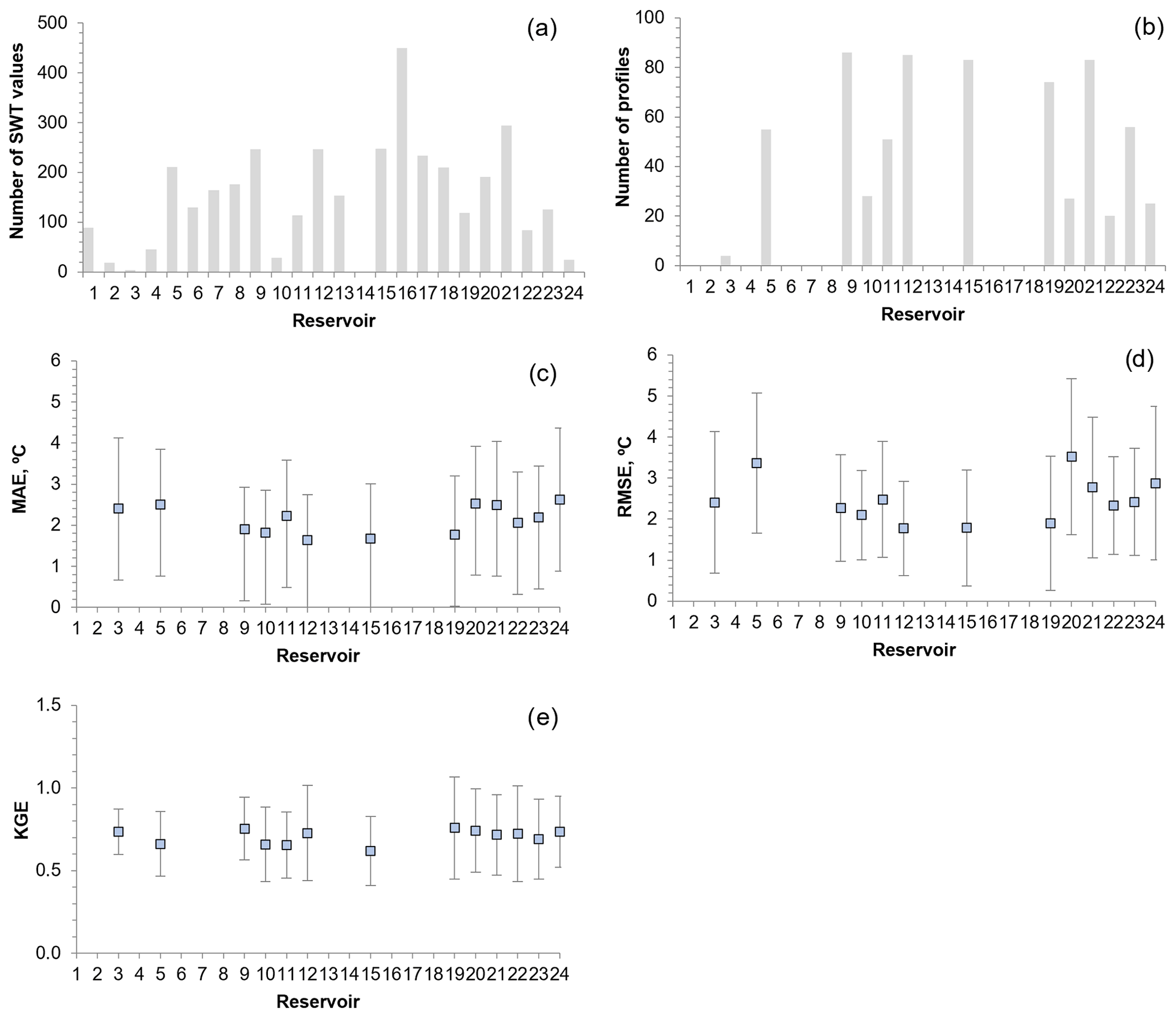
Figure 3Number of SWT values (a) and number of water temperature profiles (b) observed in the 24 reservoirs. MAE and standard deviation (c), RMSE and standard deviation (d), and KGE and standard deviation (e) between 2-D baseline scenario (W2 hydrology; daily meteorology) simulations and observed water temperature profiles.
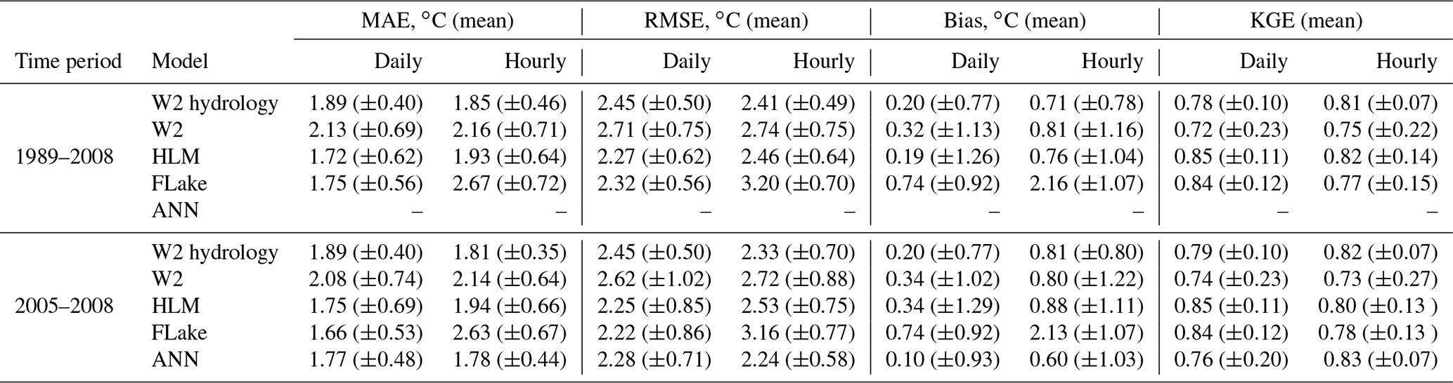
Additionally, daily and hourly SWT results were compared with the observed SWT values in order to assess the performance of the different models and the influence of the model time resolution. Simulations with the daily time step had a similar accuracy in all models (Table 5), with the HLM results being slightly closer to the observed time series. Daily metrics were obtained by comparing SWT values observed at a specific hour in the reservoirs with the daily averages obtained with the model. Therefore, they tend to level the metric results for each model, in particular the bias (Table 5). In simulations with the hourly time step, the 2-D model performed expectedly the best among the process-based models, highlighting the robustness of the baseline scenario (W2 hydrology-H). FLake had a worse performance than HLM considering the hourly results, which can be attributed to differences in the conceptualization of diurnal variations of SWT. Complete mixing within the mixed layer of FLake reduced the diurnal temperature variations (Martynov et al., 2010). The differences in the diurnal SWT variability were observed across all reservoirs.
Table 5MAE, RMSE, bias, and KGE (with standard deviation) between observed SWT values and SWT values obtained with all models, forced with daily and hourly meteorology for the 24 waterbodies.
The ANN performed best in terms of similarity to observations. The results obtained for each dataset show that the RMSE obtained with the 2-D model and with the ANN had fewer variations across all reservoirs than the results obtained with the 1-D models (Fig. 4). This result can be attributed to the wind forcing treatment by 1-D models. The latter do not consider the wind-sheltering effect, which was the most relevant parameter for calibration of the 2-D model, reducing the wind velocity by around 34 %. The response to wind stress of elongated reservoirs depends strongly on whether the dominant wind is directed across or along the reservoir main axis (Mackay, 2019). Therefore, wind direction can significantly affect SWT predictions by influencing surface mass and heat fluxes, which is evaluated in more detail in Sect. 4.3. Additionally, the comparison of W2 hydrology and W2 scenario results suggests that the SWTs of reservoirs R3, R10, and R22 were particularly affected by inflows and outflows and/or water level variations. The difference of RMSE values between W2 hydrology and W2 scenarios reached 2.7, 1.2, and 0.9 ∘C, respectively (Fig. 4).
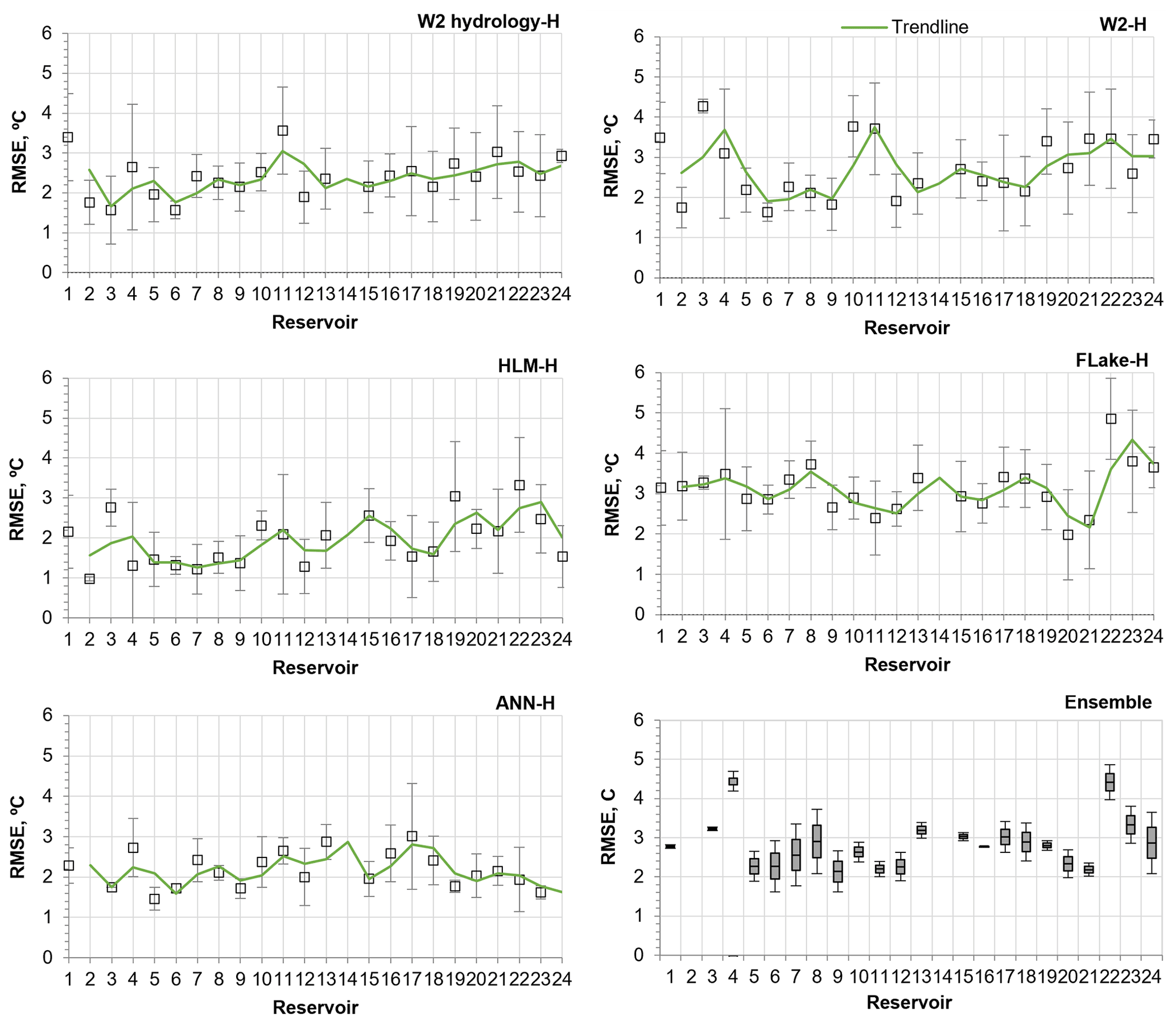
Figure 4RMSE between simulated and observed SWT time series considering hourly meteorology for the 24 waterbodies and standard deviation (time period: 1989–2008, except ANN – time period: 2005–2008). The ensemble graphic describes the mean, maximum, and minimum RMSE value obtained with the 1-D models – time period: 2005–2008 (box plot description: maximum, 75th percentile, median, 25th percentile, and minimum).
The ensemble analysis of the results obtained with the 1-D models for the period 2005–2008 (Fig. 4d) shows that the models had a similar performance. Overall, results highlight the large interannual variability of reservoir SWT and emphasize the difficulties that arise when modeling these systems.
4.2 Model intercomparison: 1-D models and the ANN
4.2.1 Model accuracy
In order to evaluate the consistency and accuracy of the models, the SWT time series were compared with the baseline scenario W2 hydrology (Table 6). When forced with hourly meteorological data, the ANN significantly reduced the error in SWT predictions for the period 2005–2008 (Fig. 5). This fact emphasizes both the potential of data-driven models to simulate the SWT and the importance of the temporal resolution of the training datasets. Overall, the ANN results remained consistent across both dry and wet seasons, reducing the annual RMSE to 0.86 ∘C (±0.31; daily meteorology) and to 0.71 ∘C (±0.21; hourly meteorology), as well as the interannual variability of RMSE. Accordingly, the KGE values are above 0.96 (Table 6).
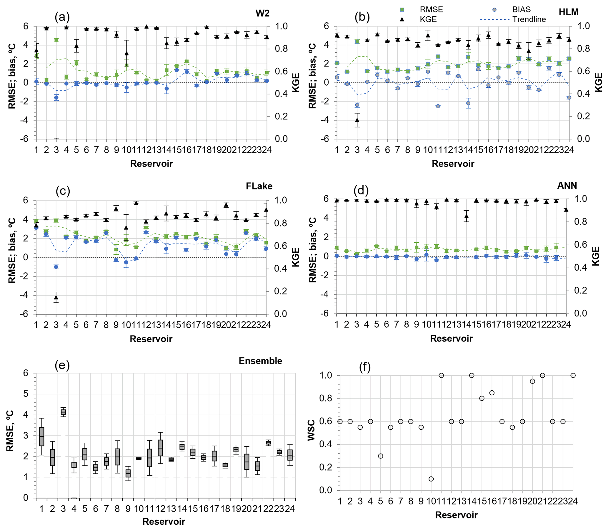
Figure 5Evaluation of simulation bias, RMSE, and KGE. 2-D baseline scenario (W2 hydrology-H) simulated SWT versus (a) the exclusion of inflows and outflows (W2-H), (b) HLM-H, (c) Flake-H, and (d) ANN-H. Models forced with hourly meteorology for the 24 waterbodies (2005–2008). The ensemble graphic in (e) shows a box plot of RMSE values (maximum, 75th percentile, median, 25th percentile, and minimum) considering the 1-D model results (2005–2008). In (f) the wind-sheltering coefficient considered during the calibration of the W2 hydrology scenario is presented.
Table 6Evaluation of model performances. 2-D baseline scenario (W2 hydrology) versus simulated SWTs with the exclusion of inflows and outflows (W2), HLM, FLake, and ANN. Models forced with daily and hourly meteorology for the 24 waterbodies (RMSE, bias, and KGE with the standard deviation).
Results of both 1-D models were similar to each other (Fig. 5), with both models reproducing the seasonal variation of SWT well and exhibiting a significant variation between the simulations performed with daily and hourly meteorological forcing and during the wet and dry seasons. Nevertheless, FLake and HLM demonstrated a reasonable performance (Table 6) similar to that reported in previous studies (Stepanenko et al., 2010, 2013; Thiery et al., 2014, 2016; Guo et al., 2021).
The two 1-D models revealed a contradictory behavior with respect to the temporal resolution. In contrast to the HLM, the FLake model had a slightly better performance with the daily than with the hourly meteorological input, which can also be attributed to differences in the conceptualization of diurnal variations of SWT. Therefore, with daily simulations, these differences between models are much less pronounced.
Considering the bias values obtained for each reservoir (Fig. 5), FLake and the HLM underestimated the SWT in 83 % and 54 % of cases, respectively. The negative SWT bias can be primarily ascribed to the overestimation by 1-D models of the wind stress effect on the surface heat flux due to ignoring the wind direction variability over wind-sheltered elongated reservoirs. The lower bias in the HLM than in FLake is more consistent with the 34 % wind velocity reduction obtained in the 2-D model calibration, suggesting that the FLake performance was affected by other factors, such as the diurnal SWT variability.
The analysis of the mean annual RMSE obtained with the HLM-H, FLake-H, and the W2-H scenarios considering the hourly meteorology indicate that Penide reservoir (R3), with a WRT of approximately 0.04 d, had the highest mean RMSE, clearly highlighting the relevance of inflows and outflows in SWTs. HLM had a worse performance for reservoirs R3, R11, R14, and R1 as well as for the six deepest reservoirs (R19, R20, R21, R22, R23, and R24), which indicates that the vertical heat diffusion was not optimally computed (Fig. 5b). Specifically, the explicit approximation of convective mixing in the HLM by convective adjustment of unstable temperature profiles is apparently too rough to simulate convective mixing in deep lakes (Bennington et al., 2014). However, it is relevant to mention that the KGE values obtained for 1-D models indicate that, overall, they performed well (Table 6). The analysis of the ensemble of RMSE results obtained with all models (Fig. 5e) reveals a high variability among SWT predictions by different models. In general, the performance of 1-D models suggests that their simplified nature and the neglect of inflows and outflows can impose high uncertainties in SWT predictions (Table 6).
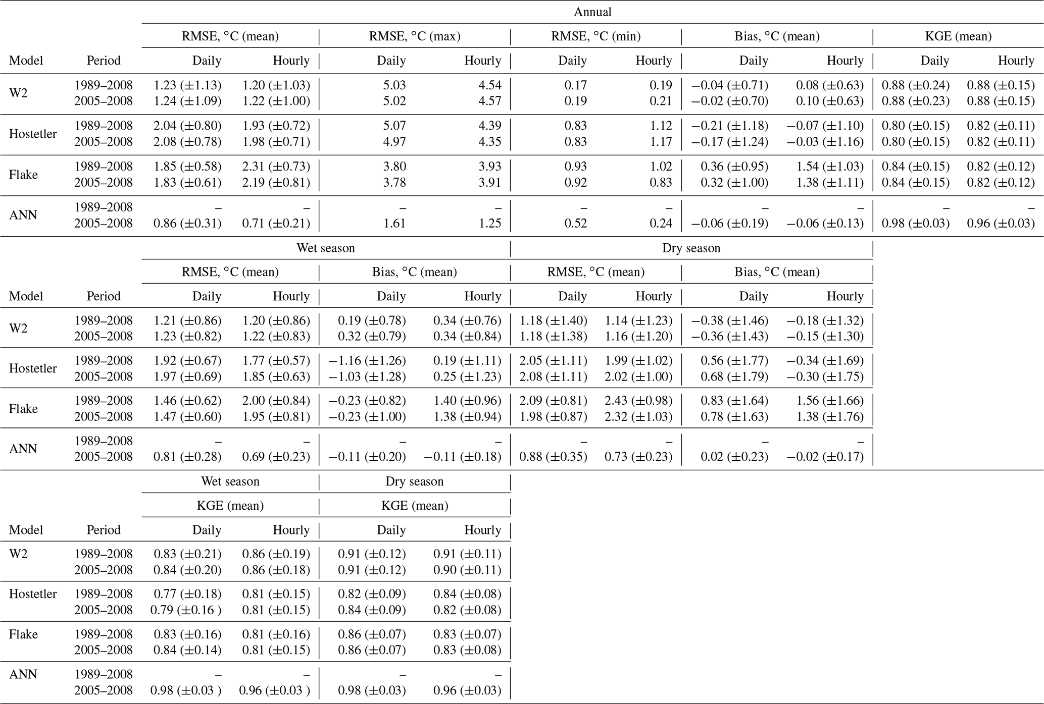
Overall, the statistical comparison by Taylor diagrams (Fig. 6) suggests that FLake had a slightly better performance than HLM in simulating SWT. It is noteworthy that the standard deviation of the simulations forced with hourly meteorology was consistently closer to the standard deviation of the baseline scenario (W2 hydrology-H) (Fig. 6c and d), showing the importance of meteorological data temporal resolution. ANN results were closer to the baseline scenario than the 2-D model (W2-H) regardless of the meteorological data discretization.
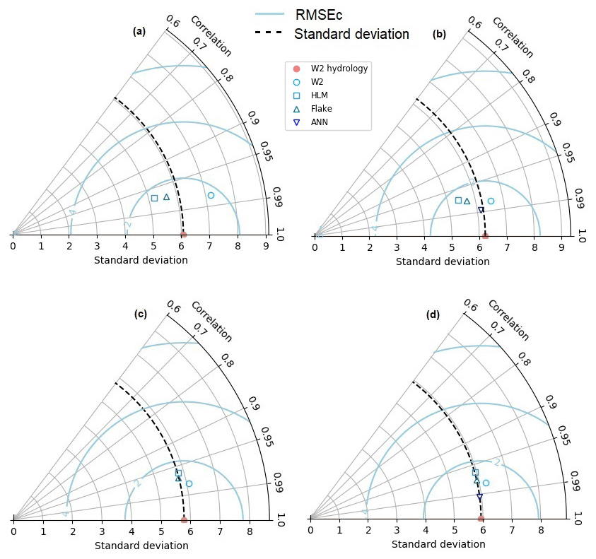
Figure 6Taylor diagrams showing the standard deviation (∘C), RMSEc (∘C), and correlation of SWT for the baseline scenario (W2 hydrology) and for each other scenario: (a) 1989–2008 (daily met.), (b) 2005–2008 (daily met.), (c) 1989–2008 (hourly met.), and (d) 2005–2008 (hourly met.). Statistics are calculated over all 24 reservoirs and lakes for the 1989–2008 period and over 22 reservoirs and lakes for the 2005–2008 period (Alqueva, R24 and Pedrógão, R14, reservoirs were not modeled with the ANN).
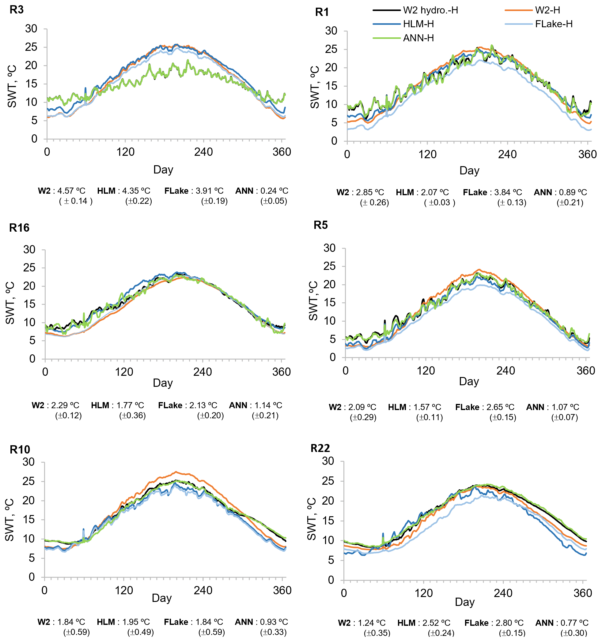
Figure 7Mean annual SWT values obtained with W2 hydrology-H (W2 hydro.-H), W2-H, HLM-H, FLake-H, and ANN-H scenarios considering hourly meteorology (2005–2008). Annual maximum RMSE between W2 hydrology-H (W2 hydro.-H) and the other scenarios' SWT results (graphics are ordered from the highest to the lowest RMSE values obtained for W2-H scenarios).
4.2.2 Modeling computation time
The analysis of computation times was conducted through the comparison of the mean CPU time per time step in the case of the 1-D models, with the mean CPU time per prediction sample obtained with the ANN, across all reservoirs. The results (Table 7) show, considering the hourly simulations, that the prediction phase of the ANN is approximately 26 times faster than FLake, the fastest process-based 1-D model optimized for coupling with climate models. The HLM code written in Python is approximately 45 times slower than FLake; nevertheless, it is important to mention that a Fortran implementation of Hostetler can be much faster as described by Thiery et al. (2016). In their work the Hostetler model was only 3.6 times slower than FLake during the modeling of a deep lake (60 m deep). Table 7 also shows the significant difference in computational time between the 2-D model and all the other models.
It is important to mention that the performance of the models depends on the software implementation; therefore, the computation time values can vary significantly from the ones presented in this research.
Table 7Computation time for process-based physical models and for the ANN prediction phase.

* The model dynamically computes a “stable” time step with the auto-stepping algorithm (vide Cole and Wells, 2008).

Figure 8Mean annual wind velocity values obtained with W2 hydrology-H (W2 hydro.-H), W2-H (accounting for the wind-sheltering effect), HLM-H, and FLake-H scenarios taking into consideration hourly meteorology (2005–2008). Bias between W2 hydrology-H and the other scenarios' mean wind velocity values.
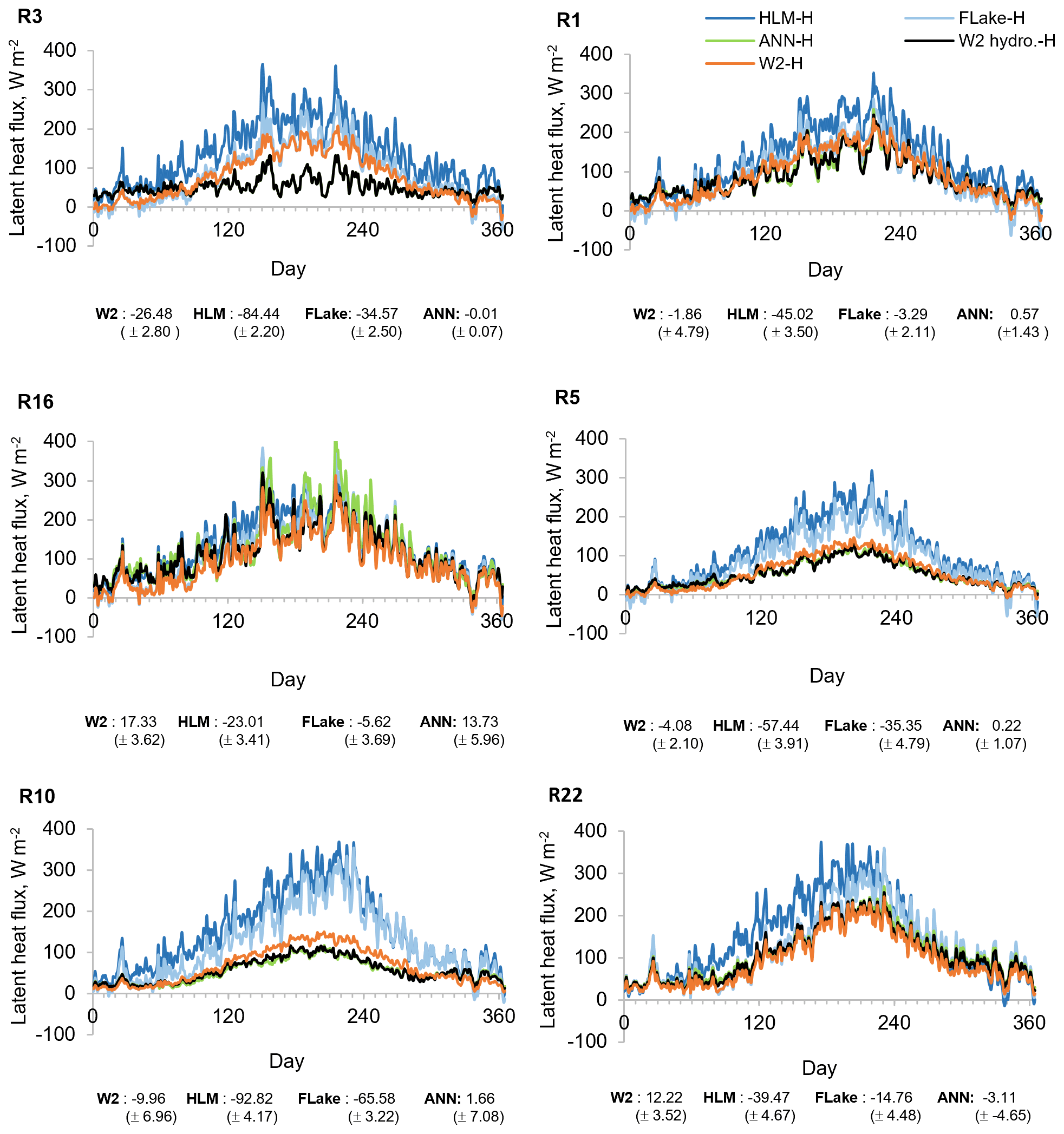
Figure 9Mean annual latent heat values obtained with W2 hydrology (W2 hydro.-H), W2 scenarios (W2-H), HLM, and FLake considering hourly meteorology (2005–2008). Bias between W2 hydrology (W2 hydro.-H) and the other models' SWT results.
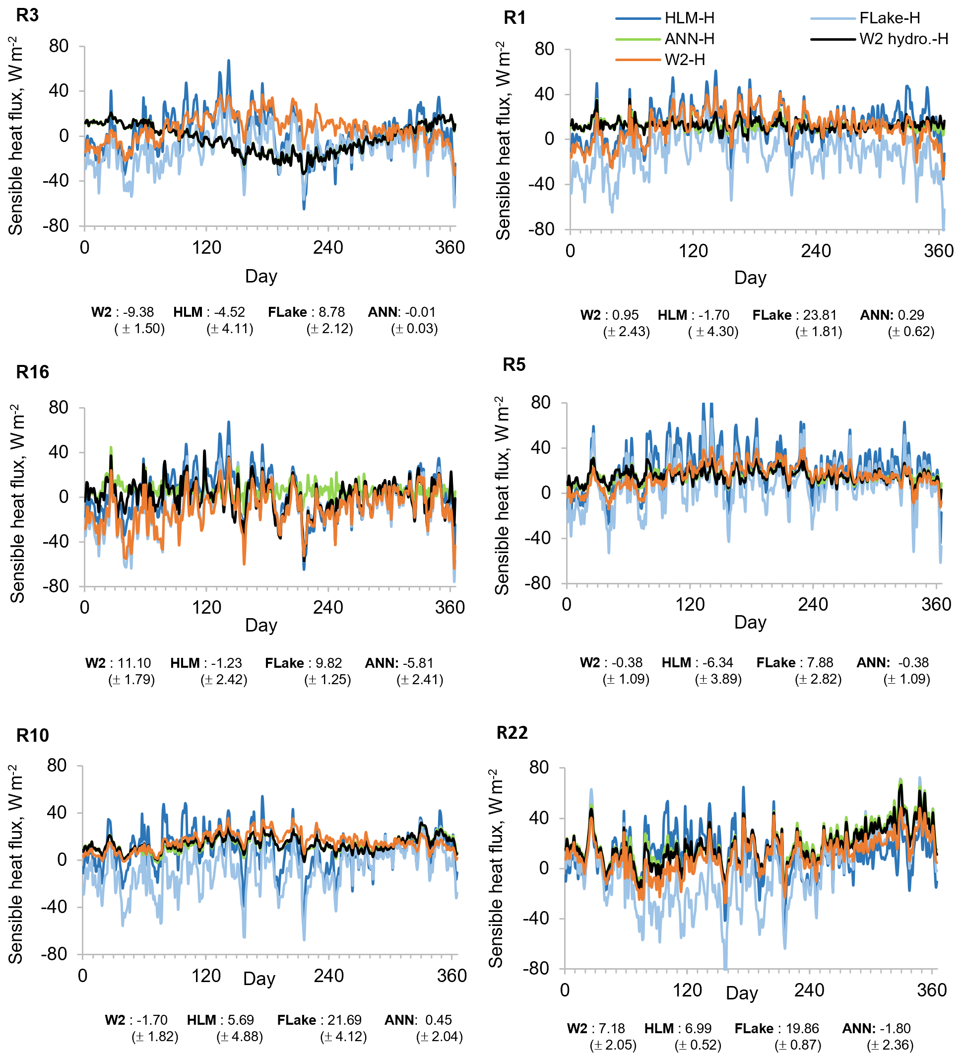
Figure 10Mean annual sensible heat values obtained with W2 hydrology (W2 hydro.-H), W2 scenarios (W2-H), HLM, and FLake considering hourly meteorology (2005–2008). Bias between W2 hydrology (W2 hydro.-H) and the other models' SWT results.
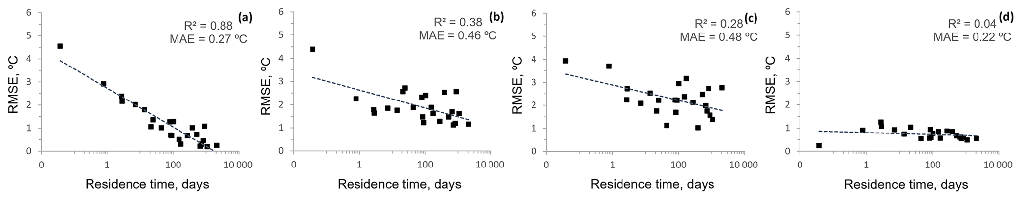
Figure 11RMSE as a function of WRT between the W2 hydrology-H scenario and simulated SWT with (a) the exclusion of inflows and outflows (W2-H, 1989–2008), (b) HLM-H (1989–2008), (c) FLake-H (1989–2008), and (d) ANN-H (2005–2008) driven with hourly meteorology.
4.3 The influence of reservoir inflows and level variations on SWT predictions
Additionally, to fully evaluate the influence of the inflows and level variations on SWT predictions in the reservoirs, and as a result on surface latent and sensible heat fluxes, we considered the mean annual SWT results obtained with all models for six reservoirs with SWT most sensitive to the exclusion of inflows and outflows. The reservoirs were chosen based on the six highest maximum RMSE values obtained between the 2-D baseline scenario (W2 hydrology-H) SWT time series and SWT time series simulated with the exclusion of inflows and outflows (W2-H) (Fig. 7). Mean annual wind velocity, surface latent heat flux, and sensible heat flux in these reservoirs are presented in Figs. 8, 9, and 10, respectively. The results for the small Penide reservoir (R3), with a maximum depth of 9 m and an average volume of 0.11 hm3, while revealing large errors in all model runs, also show that these errors were significantly improved by the ANN. The HLM overperformed the FLake model in four of the six waterbodies (R1, R16, R5, and R22). Nevertheless, both 1-D models had an overall comparable performance. The ANN significantly reduced the annual maximum RMSE obtained for all reservoirs with all the models (Fig. 7).
The aggregated analysis of results presented in Figs. 8, 9, and 10 allows estimating the combined effect of the wind forcing and the influence of inflows and level variations on the surface heat fluxes. Separation of the wind effects from the mass budget variability is possible because the differences between W2 hydrology-H and W2-H scenarios describe only the combined influence of inflows and level variations on SWT, whereas the results obtained with the 1-D models describe the joint influence of the wind forcing and the influence of inflows and level variations (Figs. 9 and 10). The results obtained for reservoirs R1, R3, R5, and R10 show an appreciable effect on the surface heat fluxes caused by the neglect of inflows. As expected, the mean annual surface heat fluxes increased and decreased during the dry and wet seasons, respectively (Figs. 9 and 10). However, results obtained with the 1-D models reveal a strong effect of the wind forcing across all reservoirs except reservoir R16. The differences in surface heat fluxes were, as expected, less pronounced in reservoir R16 due to the smaller difference between the wind forcing of the models (15 %) (Fig. 8). Generally, the 1-D models overestimated the latent heat fluxes, in particular HLM, because the FLake model results demonstrated a significant underestimation of SWT for reservoirs R1, R5, R10, and R22 as described by the corresponding maximum RMSE (Fig. 7). Accordingly, the mean annual sensible heat fluxes had a larger daily variability due to the need to balance the differences between air and water temperatures reaching 21.09 W m−2 with SD ±4.12 W m−2 (Fig. 10). The ANN significantly reduced the annual bias obtained for the surface heat fluxes for all reservoirs with all the models (Figs. 9 and 10). The only exception were the results obtained for R16, a run-of-the-river hydropower scheme for which the 2-D modeling results were strongly affected by computation instability due to large inflow values. The training of the ANN partially reflected this instability in the final ANN structure, causing a small overestimation of the surface heat fluxes during the dry season (Figs. 9 and 10).
Overall, the results show that the water level variations are clearly related to surface water temperature simulation bias; besides, the outflow (deep abstraction) reduces the volume of hypolimnion and increases the volume of the epilimnion (mixed layer) by lowering the thermocline. Herewith, water level reduction increases the area-to-the-epilimnion volume ratio, which results in an increase in epilimnetic temperature (e.g., Carr et al., 2020). The hypolimnion water temperature (HWT) was generally higher in the W2 hydrology scenarios than in the W2 scenarios due to the heat transported by interflow and underflow currents.
The differences between W2 hydrology and W2 scenarios describe the combined influence of inflows and level variations in SWT evolution quite well, which can be parameterized using the WRT. The results obtained for both scenarios reveal a significant logarithmic correlation (Eq. 11) between the RMSE of SWT from the two scenarios and WRT (Fig. 11a):
with RMSE and WRT expressed in degrees Celsius (∘C) and in days, respectively.
The results additionally show that the computed SWT values in reservoirs with a residence time shorter than 100 d may have large errors if simulated without inflows and outflows (Fig. 11).
The thermodynamics of natural and artificial lakes are similar. Nevertheless, the evolution of SWT in lakes and reservoirs differs substantially as a result of heat advection by inflows, outflows, and to a lesser extent water level variations. Evaluation of differences between thermal regimes of lakes and reservoirs from observational data is limited by the availability of comparable waterbodies. The model-based approach used in the present study provides an effective alternative that is complementary to studies evaluating the thermal structure differences between lakes (similar to a seepage lake) and reservoirs across the latitudinal gradient (e.g., Doubek and Carey, 2017; Hayes et al., 2017). We show that, for the same morphometry and under Mediterranean climatic conditions, the SWT in reservoirs (approximately 46 %) is higher than the SWT in lakes (similar to a seepage lake). The results also suggest that SWT predictions can be significantly affected by the water surface level variations. Nevertheless, in the present study only the combined effect of advection and level variation was evaluated, and the individual effect of level variations was not correlated with the SWT simulation errors. Therefore, the partial contribution of this variable to SWT was not fully explored and requires a future in-depth analysis.
One of the main novel aspects of the study lies in the fact that computationally efficient models (1-D and ANN) are compared against a baseline target instead of among themselves. Additionally, the study relies on the analysis of a large number of waterbodies and simulations conducted over a period several decades long. The methodological approach exposed the strengths and weaknesses associated with the simulation of the SWT of reservoirs by both process-based physical and data-driven models. We demonstrated that inflows and outflows have a relevant effect on the evolution of SWT, with broader implications for the quality of GCMs and RCMs used in numerical weather prediction and climate modeling. It was also shown that there are other factors besides inflows and outflows that affect SWT. Examples are the wind forcing, the temporal sampling of the meteorological forcing data, and the simplification of processes for quantifying turbulent energy flows. The low computational cost of 1-D process-based models, in particular of the FLake model, is the decisive factor for their integration in numerous GCMs and RCMs. Indeed, 1-D models such as FLake and HLM present a particularly good alternative to model reservoirs with missing field data and external parameters. Overall, Hostetler and FLake models demonstrated a reasonable performance, with the latter being slightly better in modeling SWTs. Nevertheless, the results highlight the fact that their SWT predictions can diverge significantly from observed values unless advective heat transport by inflows and outflows as well as water level variations are integrated in the models. As an alternative to process-based models, an improvement can be achieved in both accuracy and computational requirements by using data-driven models. The ANN approach demonstrated a remarkably good performance by reducing the average value of RMSE of hourly simulations by at least 64 % and running 26 times faster than the FLake model. Nevertheless, there are two important limitations to the implementation of ANNs in GCM or RCM contexts. The first is the need for a sufficient amount of accurate observational data to train the model; the second is the availability of river inflow temperatures. Both are still scarce, but their availability is rapidly increasing due to recent developments in remote sensing.
The present results suggest that reservoirs with a WRT shorter than 100 d, if simulated without representation of inflows and outflows, tend to exhibit an important deviation in the computed SWT values regardless of their morphological characteristics. Neglecting inflows and outflows while modeling these waterbodies may cause an overestimation of the turbulent energy fluxes, which can produce spurious local instabilities if surface water temperatures are higher than mean air temperatures.
Incorporation of inflows and outflows in 1-D models for regional and global climate simulations will decrease computation efficiency and add an additional layer of uncertainty in the modeling of systems whose real nature is three-dimensional. The data-driven model considered in this study outperformed process-based physical models in computation time and accuracy, being capable of accounting for the influence of inflows and outflows. In the context of waterbody simulation within numerical weather prediction and climate models, the use of data-driven approaches to complement their process-based counterparts may be highly efficient when data necessary to train the models are available. Given the growing capabilities and increasingly common use of remote sensing data acquisition techniques, the possibility of improving the performance of GCMs and RCMs through the enhanced modeling of waterbody–atmosphere turbulent heat exchanges is promising.
The exact version of the models' source code is archived on Zenodo at https://doi.org/10.5281/zenodo.4803480 (Almeida, 2021a). The current version of the open-source CE-QUAL-W2 model (version 3.6) used in this study is also available from the project website (http://www.ce.pdx.edu/w2/, last access: 5 January 2022). FLake (version 1.0) is freely available under the terms of the GNU Lesser General Public License (https://www.gnu.org/licenses/lgpl-3.0.html, last access: 5 January 2022). The model source code, a windows executable, and a comprehensive model description are freely available from the official FLake website (http://www.lakemodel.net, last access: 5 January 2022). For completeness, the Windows pre-compiled version of FLake as used in the present calculations is also archived on Zenodo (Almeida, 2021a). The open-source Hostetler model source code is also available from the repository. The Python library used to construct the ANN, NeuPy version 0.8.2, is available from the NeuPy website (http://neupy.com/pages/home.html, last access: 5 January 2022) under the terms of the MIT license, and the ANN source code and scripts used to train the model are archived on Zenodo (Almeida, 2021a).
Input files needed to run the models and the hydrometric water quality and meteorological datasets used to force and validate each model are freely available and are archived on Zenodo at https://doi.org/10.5281/zenodo.4756312 (Almeida, 2021b).
MCA conceived the study, produced the code of the Hostetler model, and performed the simulations. YS developed and optimized the ANN, while GK provided support for FLake model simulations. PMMS and RMC provided the meteorological datasets. JPM supported code development. PSC, ACR, and RMR contributed to the study design and to the results analysis. All authors contributed to the discussion and paper revision.
The contact author has declared that neither they nor their co-authors have any competing interests.
Publisher's note: Copernicus Publications remains neutral with regard to jurisdictional claims in published maps and institutional affiliations.
The authors thank the Portuguese Environmental Agency for providing the hydrometric and water quality datasets that were used in this study. Sincere thanks are given to one anonymous reviewer for the invaluable and constructive comments and suggestions for improving the paper quality. GK was partially supported by the German Research Foundation (DFG), the support of which is thankfully appreciated. The authors acknowledge FCT – Fundação para a Ciência e a Tecnologia (Portugal) through the 45 strategic project UIDB/04292/2020 granted to MARE.
This research has been supported by the German Research Foundation (DFG) (grant no. KI-853/13 and KI-853-16) and by the Fundação para a Ciência e Tecnologia (FCT) (grant no. UIDB/04292/2020).
This paper was edited by Richard Mills and reviewed by two anonymous referees.
Abadi, M., Agarwal, A., Barham, P., Brevdo, E., Chen, Z., Citro, C., Corrado, G. S., Davis, A., Dean, J., Devin, M., Ghemawat, S., Goodfellow, I. J., Harp, A., Irving, G., Isard, M., Jia, Y., Józefowicz, R., Kaiser, L., Kudlur, M., Levenberg, J., Mane, D., Monga, R., Moore, S., Murray, D. G., Olah, C., Schuster, M., Shlens, J., Steiner, B., Sutskever, I., Talwar, K., Tucker, P. A., Vanhoucke, V., Vasudevan, V., Viégas, F. B., Vinyals, O., Warden, P., Wattenberg, M., Wicke, M., Yu, Y., and Zheng, X.: TensorFlow: Large-scale machine learning on heterogeneous distributed systems, Proceedings of the 12th USENIX conference on Operating Systems Design and Implementation, Savannah, GA, USA, 2–4 November 2016, 265–283, ISBN 978-1-931971-33-1, 2016.
Almeida, M.: Models source code: CE-QUAL-W2 v3.6, FLake (windows version 1.0), Hostetler and ANN (momentum alg.) – Modeling reservoir surface temperatures for regional and global climate models (Version 1.0), Zenodo [code], https://doi.org/10.5281/zenodo.4803480, 2021a.
Almeida, M.: Model input files (hydrometric, water quality and meteorological data sets): CE-QUAL-W2 v3.6, FLake (windows version), Hostetler and ANN (momentum alg.) – Modeling reservoir surface temperatures for regional and global climate models (Version 1.0), Zenodo [data set], https://doi.org/10.5281/zenodo.4756312, 2021b.
Almeida, M. C., Coelho, P. S., Rodrigues, A. C., Diogo, P. A., Maurício, R., Cardoso, R. M., and Soares, P. M. M.: Thermal stratification of Portuguese reservoirs: Potential impact of extreme climate scenarios, J. Water Clim. Change, 6, 544–560, https://doi.org/10.2166/wcc.2015.071, 2015.
Bates, G. T., Giorgi, F., and Hostetler, S. W.: Towards the simulation of the effects of the Great Lakes on climate, Mon. Weather Rev., 121, 1373–1387, https://doi.org/10.1175/1520-0493(1993)121<1373:TTSOTE>2.0.CO;2, 1993.
Bauer, P., Thorpe, A., and Brunet, G.: The quiet revolution of numerical weather prediction, Nature, 525, 47–55, https://doi.org/10.1038/nature14956, 2015.
Bennington, V., Notaro, M., and Holman, K. D.: Improving climate sensitivity of deep lakes within a regional climate model and its impact on simulated climate, J. Climate, 27, 2886–2911, https://doi.org/10.1175/JCLI-D-13-00110.1, 2014.
Burchard, H., Bolding, K., and Villarreal, M. R.: GOTM: A General Ocean Turbulence Model: theory, implementation and test cases, Tech. Rep. EUR 18745 EN, European Commission, Joint Research Center, Space Applications Institute, 1999.
Calamita, E., Sebastiano Piccolroaz, S., Majone, B., and Toffolon, M.: On the role of local depth and latitude on surface warming heterogeneity in the Laurentian Great Lakes, Inland Waters, 11, 208–222, https://doi.org/10.1080/20442041.2021.1873698, 2021.
Cardoso, R. M., Soares, P. M. M., Miranda, P. M. A., and Belo-Pereira, M.: WRF High resolution simulation of Iberian mean and extreme precipitation climate, Int. J. Climatol., 33, 2591–2608, https://doi.org/10.1002/joc.3616, 2013.
Carr, M. K., Sadeghian, A., Lindenschmidt, Karl-Erich, Rinke, K., and Morales-Marin, L.: Impacts of Varying Dam Outflow Elevations on Water Temperature, Dissolved Oxygen, and Nutrient Distributions in a Large Prairie Reservoir, Environ. Eng. Sci., 37, 78–79, https://doi.org/10.1089/ees.2019.0146, 2020.
Chenard, J. F. and Caissie, D.: Stream temperature modelling using artificial neural networks: application on Catamaran Brook, New Brunswick, Canada, Hydrol. Process., 22, 3361–3372, https://doi.org/10.1002/hyp.6928, 2008.
Cole, T. M. and Wells, S. A.: CE-QUAL-W2: A Two- Dimensional, Laterally Averaged, Hydrodynamic and Water Quality Model, Version 3.6, User manual, Report of Department of Civil and Environmental Engineering, Portland State University, Portland, OR, 797, available at: http://www.ce.pdx.edu/w2/ (last access: 5 January 2022), 2008.
Deng, B., Liu, S., Xiao, W., Wang, W., Jin, J., and Lee, X.: Evaluation of the CLM4 Lake Model at a Large and Shallow Freshwater Lake, J. Hydrometeorol., 14, 636–649, https://doi.org/10.1175/JHM-D-12-067.1, 2013.
Diogo, P. A., Fonseca, M., Coelho, P., Mateus, N., Almeida, M., and Rodrigues, A.: Reservoir phosphorous sources evaluation and water quality modeling in a transboundary watershed, Desalination, 226, 200–214, https://doi.org/10.1016/j.desal.2007.01.242, 2008.
Doubek, J. P. and Carey, C. C.: Catchment, morphometric, and water quality characteristics differ between reservoirs and naturally formed lakes on a latitudinal gradient in the conterminous United States, Inland Waters, 7, 171–180, https://doi.org/10.1080/20442041.2017.1293317, 2017.
Dutra, E., Stepanenko, V. M., Balsamo, G., Viterbo, P., Miranda, P., Mironov, D., and Schär, C.: An offline study of the impact of lakes in the performance of the ECMWF surface scheme boreal, Environ. Res., 15, 100–112, 2010.
Edinger, J. E., Duttweiler, D. W., and Geyer, J. C.: The response of water temperature to meteorological conditions, Water Resour. Res., 4, 1137–1143, https://doi.org/10.1029/WR004i005p01137, 1968.
Fang, X. and Stefan, H. G.: Long-term lake water temperature and ice cover simulations/measurements, Cold Reg. Sci. Technol., 24, 289–304, https://doi.org/10.1016/0165-232X(95)00019-8, 1996.
Flato, G., J., Marotzke, B., Abiodun, P., Braconnot, S. C., Chou, W., Collins, P., Cox, F., Driouech, S., Emori, V., Eyring, C., Forest, P., Gleckler, E., Guilyardi, C., Jakob, V., Kattsov, C., Reason, and Rummukainen, M.: Evaluation of Climate Models, in: Climate Change 2013: The Physical Science Basis. Contribution of Working Group I to the Fifth Assessment Report of the Intergovernmental Panel on Climate Change, edited by: Stocker, T. F., Qin, D., Plattner, G. K., Tignor, M., Allen, S. K., Boschung, J., Nauels, A., Xia, Y., Bex, V., and Midgley, P. M., Cambridge University Press, Cambridge, United Kingdom and New York, NY, USA, 578–635, ISBN 978-1-107-05799-1, 2013.
Forster, P.: Half a century of robust climate models, Nature, 545, 296–297, https://doi.org/10.1038/545296a, 2017.
Friedrich, K., Grossman, R. L., Huntington, J., Blanken, P. D., Lenters, J., Holman, K. D., Gochis, D., Livneh, B., Prairie, J., Skeie, E., Healey, N. C, Dahm, K., Pearson, C., Finnessey, T., Hook, S. J., and Kowalski T.: Reservoir Evaporation in the Western United States: Current Science, Challenges, and Future Needs, B. Am. Meteorol. Soc., 99, 167–187, https://doi.org/10.1175/BAMS-D-15-00224.1, 2018.
Goudsmit, G. H., Burchard, H., Peeters, F., and Wüest, A.: Application of k–turbulence models to enclosed basins: The role of internal seiches, J. Geophys. Res., 107, 3230, https://doi.org/10.1029/2001JC000954, 2002.
Gu, H., Jin, J., Wu, Y., Ek, M. B., and Subin, Z. M.: Calibration and validation of lake surface temperature simulations with the coupled WRF-lake model, Climatic Change, 129, 471–483, https://doi.org/10.1007/s10584-013-0978-y, 2015.
Gula, J. and Peltier, W. R.: Dynamical Downscaling over the Great Lakes Basin of North America Using the WRF Regional Climate Model: The Impact of the Great Lakes System on Regional Greenhouse Warming, J. Climate, 25, 7723–7742, https://doi.org/10.1175/JCLI-D-11-00388.1, 2012.
Guo, M., Zhuang, Q., Yao, H., Golub, M., Leung, L. R., Pierson, D., and Tan, Z.: Validation and Sensitivity Analysis of a 1-D Lake Model Across Global Lakes, J. Geophys. Res.-Atmos., 126, e2020JD033417, https://doi.org/10.1029/2020JD033417, 2021.
Guseva, S., Bleninger, T., Jöhnk, K., Polli, B. A., Tan, Z., Thiery, W., Zhuang, Q., Rusak, J. A., Yao, H., Lorke, A., and Stepanenko, V.: Multimodel simulation of vertical gas transfer in a temperate lake, Hydrol. Earth Syst. Sci., 24, 697–715, https://doi.org/10.5194/hess-24-697-2020, 2020.
Hayes, N. M., Deemer, B. M., Corman, J. R., Razavi, N. R., and Strock, K. E.: Key differences between lakes and reservoirs modify climate signals: A case for a new conceptual model, Limnol. Oceanogr. Lett., 2, 47–62, https://doi.org/10.1002/lol2.10036, 2017.
Hebert, C., Caissie, D., Satish, M., and El-Jabi, N.: Modeling of hourly river water temperature using artificial neural networks, Water Qual. Res. J. Can., 49, 144–162, https://doi.org/10.2166/wqrjc.2014.007, 2014.
Henderson-Sellers, B.: New formulation of eddy diffusion thermocline models, Appl. Math. Model., 9, 441–446, https://doi.org/10.1016/0307-904X(85)90110-6, 1985.
Hipsey, M. R., Bruce, L. C., Boon, C., Busch, B., Carey, C. C., Hamilton, D. P., Hanson, P. C., Read, J. S., de Sousa, E., Weber, M., and Winslow, L. A.: A General Lake Model (GLM 3.0) for linking with high-frequency sensor data from the Global Lake Ecological Observatory Network (GLEON), Geosci. Model Dev., 12, 473–523, https://doi.org/10.5194/gmd-12-473-2019, 2019.
Hostetler, S. and Bartlein, P. J.: Simulation of lake evaporation with application to modeling lake-level variations at Harney-Malheur Lake, Oregon, Water Resour. Res., 26, 2603–2612, https://doi.org/10.1029/WR026i010p02603, 1990.
Hostetler, S. W. and Giorgi, F.: Effects of a 2×3 CO2 climate on two large lake systems: Pyramid Lake, Nevada, and Yellowstone Lake, Wyoming, Global Planet. Change, 10, 43–54, https://doi.org/10.1016/0921-8181(94)00019-A, 1995.
Huang, A., Lazhu, Wang, J., Dai, Y., Yang, K., Wei, N., Wen, L., Wu, Y., Zhu, X., Zhang, X., and Cai, S.: Evaluating and improving the performance of three 1‐D Lake models in a large deep Lake of the central Tibetan Plateau, J. Geophys. Res., 124, 3143–3167. https://doi.org/10.1029/2018JD029610, 2019.
Irambona, C., Music, B., Nadeau, D. F., Mahdi, T. F., and Strachan, I. B.: Impacts of boreal hydroelectric reservoirs on seasonal climate and precipitation recycling as simulated by the CRCM5: a case study of the La Grande River watershed, Canada, Theor. Appl. Climatol., 131, 1529–1544, https://doi.org/10.1007/s00704-016-2010-8, 2018.
Jacob, D., Teichmann, C., Sobolowski, S., Katragkou, E., Anders, I., Belda, M., Benestad, R., Boberg, F., Buonomo, E., Cardoso, R. M., Casanueva, A., Christensen, O. B., Christensen, J. H., Coppola, E., De Cruz, L., Davin E. L., Dobler, A., Domínguez, M., Fealy, R., Fernandez, J., Gaertner, M. A., García-Díez, M., Giorgi, F., Gobiet, A., Goergen, K., Gómez-Navarro, J. J., Alemán, J. J. G. , Gutiérrez, C., Gutiérrez J. M., Güttler, I., Haensler, A., Halenka, T., Jerez, S., Jiménez-Guerrero, P., Jones, R. G., Keuler, K., Kjellström, E., Knist, S., Kotlarski, S., Maraun, D., van Meijgaard, E., Mercogliano, P., Montávez, J. P., Navarra, A., Nikulin, G., de Noblet-Ducoudré, N., Panitz, H. J. , Pfeifer, S., Piazza, M., Pichelli, E., Pietikäinen, J. P., Prein, A. F., Preuschmann, S., Rechid, D., Rockel, B., Romera, R., Sánchez, E., Sieck, K., Soares, P. M. M. , Somot, S., Srnec, L., Sørland, S. L., Termonia, P., Truhetz, H., Vautard, R., Warrach-Sagi, and K., Wulfmeyer, V.: Regional climate downscaling over Europe: perspectives from the EURO-CORDEX community, Reg. Environ. Change., 20, 51, https://doi.org/10.1007/s10113-020-01606-9, 2020..
Karagounis, I., Trösch, J., and Zamboni, F.: A coupled physical-biochemical lake model for forecasting water quality, Aquat. Sci., 55, 87–102, https://doi.org/10.1007/BF00877438, 1993.
Kirillin, G.: Modeling the impact of global warming on water temperature and seasonal mixing regimes in small temperate lakes, Boreal Environ. Res., 15, 279–293, 2010.
Kitaigorodskii, S. A. and Miropolsky, Y.: On the theory of the open ocean active layer, Atmos. Ocean. Phys., 6, 178–188, 1970.
Kling, H., Fuchs, M., and Paulin, M.: Runoff conditions in the upper Danube basin under an ensemble of climate change scenarios, J. Hydrol., 424–425, 264–277, https://doi.org/10.1016/j.jhydrol.2012.01.011, 2012.
Kraus, E. B. and Turner, J. S.: A one-dimensional model of the seasonal thermocline II. The general theory and its consequences, Tellus, 19, 98–106, https://doi.org/10.1111/j.2153-3490.1967.tb01462.x, 1967.
Le Moigne, P., Colin, J., and Decharme B.: Impact of lake surface temperatures simulated by the FLake scheme in the CNRM-CM5 climate model, Tellus A, 68, 31274, https://doi.org/10.3402/tellusa.v68.31274, 2016.
Ljungemyr, P., Gustafsson, N., and Omstedt, A.: Parameterization of lake thermodynamics in a high-resolution weather forecasting model, Tellus A, 48, 608–621, https://doi.org/10.3402/tellusa.v48i5.12155, 1996.
Lofgren B.: Land Surface Roughness Effects on Lake Effect Precipitation, J. Great Lakes Res., 32, 839–851, https://doi.org/10.3394/0380-1330(2006)32[839:LSREOL]2.0.CO;2, 2006.
Long, Z., Perrie, W., Gyakum, J., Caya, D., and Laprise, R.: Northern Lake Impacts on Local Seasonal Climate, J. Hydrometeorol., 8, 881–896, https://doi.org/10.1175/JHM591.1, 2007.
MacKay, M. D.: Incorporating wind sheltering and sediment heat flux into 1-D models of small boreal lakes: a case study with the Canadian Small Lake Model V2.0, Geosci. Model Dev., 12, 3045–3054, https://doi.org/10.5194/gmd-12-3045-2019, 2019.
Magee, M. R. and Wu, C. H.: Response of water temperatures and stratification to changing climate in three lakes with different morphometry, Hydrol. Earth Syst. Sci., 21, 6253–6274, https://doi.org/10.5194/hess-21-6253-2017, 2017.
Martinov, A., Sushama L., and Laprise, R.: Simulation of temperate freezing lakes by one-dimensional lake models: performance assessment for interactive coupling with regional climate models, Boreal Environ. Res., 15, 143–164, 2010.
Mironov, D., Heise, E., Kourzeneva, E., Ritter, B., Schneider, N., and Terzhevik, A.: Implementation of the lake parameterisation scheme FLake into the numerical weather prediction model COSMO, Boreal. Environ. Res. 15, 218–230, 2010.
Niziol, T. A., Snyder, W. R., and Waldstreicher, J. S.: Winter Weather Forecasting throughout the Eastern United States. Part IV: Lake Effect Snow, Weather Forecast., 10, 61–77, https://doi.org/10.1175/1520-0434(1995)010<0061:WWFTTE>2.0.CO;2, 1995.
Nogueira, M., Soares, P. M. M., Tomé, R., and Cardoso, R. M.: High-resolution multi-model projections of onshore wind resources over Portugal under a changing climate, Theor. Appl. Climatol., 136, 347–362, https://doi.org/10.1007/s00704-018-2495-4, 2019.
Nordbo, A., Launiainen, S., Mammarella, I., Leppäranta, M., Huotari, J., Ojala, A., and Vesala, T.: Long-term energy flux measurements and energy balance over a small boreal lake using eddy covariance technique, J. Geophys Res, 116, D02119, https://doi.org/10.1029/2010JD014542, 2011.
Notaro, M., Zarrin, A., Vavrus, S., and Bennington, V.: Simulation of heavy lake-effect snowstorms across the Great Lakes basin by RegCM4: Synoptic climatology and variability, Mon. Weather Rev., 141, 1990–2014, https://doi.org/10.1175/MWR-D-11-00369.1, 2013.
OECD (Eds.): Eutrophication of waters – Monitoring Assessment and control, Organization for the Economic Cooperation and Development, OECD, Paris, 154, ISBN 92-64-22298-7, 1982.
Oleson, K. W., Dai, Y., Bonan, G. B., Bosilovich, M., Dickinson, R., Dirmeyer P., Hoffman F., Houser, P., Levis, S., Niu, G., Thornton, P., Vertenstein M., Yang, Z., and Zeng, X.: Technical Description of the Community Land Model (CLM), NCAR Technical Note NCARTN-461+STR, National Center for Atmospheric Research, Boulder, Colorado, 174, https://doi.org/10.5065/D6N877R0, 2004.
Oswald, C. J. and Rouse, W. R.: Thermal Characteristics and Energy Balance of Various-Size Canadian Shield Lakes in the Mackenzie River Basin, J. Hydrometeorol., 5, 129–144, https://doi.org/10.1175/1525-7541(2004)005<0129:TCAEBO>2.0.CO;2, 2004.
Perroud, M., Goyette, S., Martynov, A., Beniston, M., and Annevillec, O.: Simulation of multiannual thermal profiles in deep Lake Geneva: a comparison of onedimensional lake models, Limnol. Oceanogr., 54, 1574–1594, https://doi.org/10.4319/lo.2009.54.5.1574, 2009.
Philips, D. W.: Modification of surface air over Lake Ontario in Winter, Mon. Weather Rev., 100, 662–670, https://doi.org/10.1175/1520-0493(1972)100<0662:MOSAOL>2.3.CO;2, 1972.
Qian, N.: On the momentum term in gradient descent learning algorithms, Neural Networks, 12, 145–151, https://doi.org/10.1016/S0893-6080(98)00116-6, 1999.
Read, J. S., Jia, X., Willard, J., Appling, A. P., Zwart, J. A., Oliver, S. K., Karpatne, A., Hansen, G., Hansin, P., Watkins W., Steinbach, M., and Kumar, V.: Process-guided deep learning predictions of lake water temperature, Water Resour. Res., 55, 9173–9190, https://doi.org/10.1029/2019WR024922, 2019.
Rijo, N., Lima, D. C. A., Semedo, A., Miranda, P. M. A., Cardoso, R. M., and Soares, P. M. M.: Spatial and Temporal Variability of the Iberian Peninsula Coastal Low-Level Jet, Int. J. Climatol., 38, 1605–1622, https://doi.org/10.1002/joc.5303, 2018.
Rimmer, A., Gal, G., Opher, T., Lechinsky, Y., and Yacobi, Y. Z.: Mechanisms of long-term variations in the thermal structure of a warm lake, Limnol. Oceanogr., 56, 974–988, https://doi.org/10.4319/lo.2011.56.3.0974, 2011.
Rouse, W., Oswald, C., Binyamin, J., Blanken, P., Schertzer, W., and Spence, C.: Interannual and Seasonal Variability of the Surface Energy Balance and Temperature of Central Great Slave Lake, J. Hydrometeorol., 4, 720–730, https://doi.org/10.1175/1525-7541(2003)004<0720:IASVOT>2.0.CO;2, 2003.
Samadianfard, S., Kazemi, H., Kisi, O., and Liu W.: Water temperature prediction in a subtropical subalpine lake using soft computing techniques, Earth Sci. Res. J., 20, 2, https://doi.org/10.15446/esrj.v20n2.43199, 2016.
Samuelsson, P., Kourzeneva, E., and Mironov, D.: The impact of lakes on the European climate as simulated by a regional climate model, Boreal. Environ. Res., 15, 113–129, 2010.
Schertzer, W. M.: Freshwater lakes, in: The Surface Climates of Canada, edited by: Bailey, W. G., Oke, T. R., and Rouse, W. R., McGill-Queen's University Press, Montreal and Kingston, London, 124–148, ISBN 9780773516724, 1997.
Sharma, S., Walker, S. C., and Jackson, D. A.: Empirical modelling of lake water-temperature relationships: A comparison of approaches, Freshwater Biol., 53, 897–911, https://doi.org/10.1111/j.1365-2427.2008.01943.x, 2008.
Shatwell, T., Thiery, W., and Kirillin, G.: Future projections of temperature and mixing regime of European temperate lakes, Hydrol. Earth Syst. Sci., 23, 1533–1551, https://doi.org/10.5194/hess-23-1533-2019, 2019.
Shevchuk, Y.: Python library, available at: http://neupy.com/pages/home.html (last access: 5 January 2022), 2015.
Skamarock, W. C., Klemp, J. B., Dudhia, J., Gill, D. O., Barker, D. M., Duda, M. G., Huang, X., Wang, W., and Powers, J. G.: A description of the advanced research WRF, Version 3, Technical report (No. NCAR/TN-475+STR), University Corporation for Atmospheric Research, https://doi.org/10.5065/D68S4MVH, 2008.
Soares, P. M. M., Cardoso, R. M., Medeiros, J., Miranda, P. M. A., Belo-Pereira, M., and Espirito-Santo, F.: WRF High resolution dynamical downscaling of ERA-Interim for Portugal, Climate Dynamics, 39, 2497–2522, https://doi.org/10.1007/s00382-012-1315-2#Bib1, 2012a.
Soares, P. M. M., Cardoso, R. M., Miranda, P. M. A., Viterbo, P., and Belo-Pereira, M.: Assessment of the ENSEMBLES regional climate models in the representation of precipitation variability and extremes over Portugal, J. Geophys. Res., 117, 7, https://doi.org/10.1029/2011JD016768, 2012b.
Soares, P. M. M., Cardoso, R. M., Semedo, A., Chinita, M. J., and Ranjha, R.: Climatology of Iberia Coastal Low-Level Wind Jet: WRF High Resolution Results, Tellus A, 66, 1, https://doi.org/10.3402/tellusa.v66.22377, 2014.
Stepanenko, V. M. and Lykossov, V. N.: Numerical modeling of heat and moisture transfer processes in a system lake–soil, Russ. Meteorol. Hydrol., 3, 95–104, 2005.
Stepanenko, V. M., Goyette, S., Martynov, A., Perroud M., Fang, X., and Mironov A.: First steps of a lake model intercomparison Project: LakeMIP, Boreal Environ. Res., 15, 191–202, 2010.
Stepanenko, V. M., Martynov, A., Jöhnk, K. D., Subin, Z. M., Perroud, M., Fang, X., Beyrich, F., Mironov, D., and Goyette, S.: A one-dimensional model intercomparison study of thermal regime of a shallow, turbid midlatitude lake, Geosci. Model Dev., 6, 1337–1352, https://doi.org/10.5194/gmd-6-1337-2013, 2013.
Subin, Z. M., Riley, W. J., and Mironov, D.: An improved lake model for climate simulations: Model structure, evaluation, and sensitivity analyses in CESM1, J. Adv. Model. Earth Sy., 4, 1, https://doi.org/10.1029/2011MS000072, 2012.
Svensson, U.: A mathematical model of the seasonal thermocline, Ph.D. thesis, Lund Institute of Technology, Lund, 1978.
Thackston, E. L. and Parker, F. L.: Effect of Geographical Location on Cooling Pond Requirements and Performance, water Pollution Control Research Series 16130 FDQ 03/71, Vanderbilt University, Dept. of Environmental and Water Resources Engineering, Environmental Protection Agency (EPA), Washington, D. C., 244, 1971.
Thiery, W., Martynov, A., Darchambeau, F., Descy, J.-P., Plisnier, P.-D., Sushama, L., and van Lipzig, N. P. M.: Understanding the performance of the FLake model over two African Great Lakes, Geosci. Model Dev., 7, 317–337, https://doi.org/10.5194/gmd-7-317-2014, 2014.
Thiery, W., Stepanenko, V. M., Fang, X., Jöhnk, K. D., Li, Z., Martynov, A., Perroud, M., Subin, Z. M., Darchambeau, F., Mironov, D., and Van Lipzig, N. P. M.: LakeMIP Kivu: evaluating the representation of a large, deep tropical lake by a set 835 of one-dimensional lake models, Tellus A, 66, 1, https://doi.org/10.3402/tellusa.v66.21390, 2016.
Toffolon, M. and Piccolroaz, S.: A hybrid model for river water temperature as a function of air temperature and discharge, Environ. Res. Lett., 10, 114011, https://doi.org/10.1088/1748-9326/10/11/114011, 2015.
Wang, F., Ni, G., Riley, W. J., Tang, J., Zhu, D., and Sun, T.: Evaluation of the WRF lake module (v1.0) and its improvements at a deep reservoir, Geosci. Model Dev., 12, 2119–2138, https://doi.org/10.5194/gmd-12-2119-2019, 2019.
Wang, Y., Ma, Q., Gao, Y., Hao, X., and Liu, S.: Simulation of the surface energy flux and thermal stratification of lake Taihu with three 1-D models, Water, 11, 1026, https://doi.org/10.3390/w11051026, 2019.
Wright, D. M., Posselt, D. J., and Steiner, A. L.: Sensitivity of Lake-Effect Snowfall to Lake Ice Cover and Temperature in the Great Lakes Region, Mon. Weather Rev., 141, 670–689, https://doi.org/10.1175/MWR-D-12-00038.1, 2013.
Wunderlich, W.: Heat and Mass Transfer between a Water Surface and the Atmosphere, Rpt. No. 14, Rpt. Publication No. 0-6803, Water Resources Research Laboratory, Tennessee Valley Authority, Division of Water Control Planning, Engineering Laboratory, Norris, TN, 1972.
Xiao, C., Lofgren, B., Wang, J., and Chu, P.: Improving the lake scheme within a coupled WRF-Lake model in the Laurentian Great Lakes, J. Adv. Model. Earth Sy., 8, 4, https://doi.org/10.1002/2016MS000717, 2016.
Xue, P., Pal, J. S., Ye, X., Lenters, J. D., Huang, C., and Chu, P. Y.: Improving the simulation of large lakes in regional climate modeling: Two-way lake–atmosphere coupling with a 3D hydrodynamic model of the Great Lakes, J. Climate, 30, 1605–1627, https://doi.org/10.1175/JCLI-D-16-0225.1 2017.
Zamboni, F., Barbieri, A., Polli, B., Salvadè, G., and Simona, M.: The dynamic model SEEMOD applied to the southern basin of lake Lugano, Aquat. Sci., 54, 367–380, https://doi.org/10.1007/BF00878148, 1992.