Using neural network ensembles to separate ocean biogeochemical and physical drivers of phytoplankton biogeography in Earth system models

Earth system models (ESMs) are useful tools for predicting and understanding past and future aspects of the climate system. However, the biological and physical parameters used in ESMs can have wide variations in their estimates. Even small changes in these parameters can yield unexpected results without a clear explanation of how a particular outcome was reached. The standard method for estimating ESM sensitivity is to compare spatiotemporal distributions of variables from different runs of a single ESM. However, a potential pitfall of this method is that ESM output could match observational patterns because of compensating errors. For example, if a model predicts overly weak upwelling and low nutrient concentrations, it might compensate for this by allowing phytoplankton to have a high sensitivity to nutrients. Recently, we demonstrated that neural network ensembles (NNEs) are capable of extracting relationships between predictor and target variables within ocean biogeochemical models. Being able to view the relationships between variables, along with spatiotemporal distributions, allows for a more mechanistically based examination of ESM outputs. Here, we investigated whether we could apply NNEs to help us determine why different ESMs produce different spatiotemporal distributions of phytoplankton biomass. We tested this using three cases. The first and second case used different runs of the same ESM, except that the physical circulations differed between them in the first case, while the biological equations differed between them in the second. Our results indicated that the NNEs were capable of extracting the relationships between variables for different runs of a single ESM, allowing us to distinguish between differences due to changes in circulation (which do not change relationships) from changes in biogeochemical formulation (which do change relationships). In the third case, we applied NNEs to two different ESMs. The results of the third case highlighted the capability of NNEs to contrast the apparent relationships of different ESMs and some of the challenges it presents. Although applied specifically to the ocean components of an ESM, our study demonstrates that Earth system modelers can use NNEs to separate the contributions of different components of ESMs. Specifically, this allows modelers to compare the apparent relationships across different ESMs and observational datasets.

1 Introduction

Earth system models (ESMs) are increasingly used to help us understand how anthropogenic greenhouse gas emissions will affect biological systems and how such changes will feed back on the climate system. Although these methods provide an avenue for examining processes on a global scale, their representations of biological and physical processes of the natural world are limited by imperfect knowledge and the inability to resolve these processes with current models, which require ever increasingly higher computational costs for additional complexity and resolution. As a result, estimates of critical biological and physical parameters can vary quite substantially. For example, from tracer experiments in the North Atlantic subtropical gyre, diapycnal diffusivity was estimated between 0.1 and 0.5 cm² s⁻¹ (Ledwell et al., 1998), with similar values having been used in ESMs. Varying the diapycnal diffusivity within this range in ESMs has been shown to yield different results in the biogeochemical output (Oschlies, 2001; Duteil and Oschlies, 2011). Furthermore, ESMs do not agree about how to represent phytoplankton growth parameters, such as temperature dependence. In the nine ESMs compared in Laufkötter et al. (2015), the Q₁₀ value describing the sensitivity of growth rate to 10^∘ increases in temperature ranged from 1.68 to 3, with some models varying the Q₁₀ values based on the size or type of phytoplankton.

The uncertainty associated with some ESM parameters can make it difficult to understand why different ESMs may yield different predictions for biological variables ranging from productivity to carbon uptake. Bopp et al. (2013) demonstrated that while CMIP5 models showed the same overall global trends under climate change for variables such as pH, sea surface temperature, O₂, and primary productivity, there were substantial cross-model differences in O₂ and primary productivity on regional scales.

Traditional methods used to estimate the sensitivity of ESMs often compare the spatial distributions of biological and physical variables from different runs of a single ESM to each other or to observations. However, occasionally changes in one parameter improve the simulation of one variable while degrading the simulation of another (see, for example, Bahl et al., 2019, their Table 2). Other times, errors in one variable are due to errors in another (i.e., getting a physical front in the wrong place may mean that the biomass has the wrong distribution).

The intent of ESMs is to get the correct spatial distribution both because the correct relationships between environmental predictors and target variables are being modeled and because the environmental predictors themselves are correctly modeled. However, it is difficult to know if the correct relationships are indeed being modeled. Thus, a method is needed with which we can evaluate whether different ESMs yield different projections because of fundamental differences in biogeochemical formulation or whether such differences are primarily due to differences in physical circulations and climate sensitivities. Of the potential methods available, neural network ensembles (NNEs) are a strong candidate. NNEs are a machine learning (ML) technique which use the average of many individual neural networks (NNs) to predict the outcome of datasets. The objective of this paper is to investigate whether the application of NNEs and sensitivity analyses can provide useful information for determining the most substantial sources of differences in ESM outputs.

We previously demonstrated that NNEs were able to extract relationships between biological forcings and outputs within a simplified biogeochemical model (Holder and Gnanadesikan, 2021). NNEs were able to outperform other ML algorithms, such as random forests. More importantly, NNEs also had the benefits of being able to extrapolate outside the range of the training dataset and to provide a measure of their uncertainty in their predictions. In Holder and Gnanadesikan (2021), we defined two types of relationships between environmental forcings and biological responses: intrinsic and apparent. Intrinsic relationships are those in which the effect of one predictor variable on an outcome (target variable) can be examined, while maintaining other predictors at a constant level. An example of this would be the results of a laboratory experiment examining how the growth rate of a particular species of phytoplankton depends on different nutrient concentrations, while all other factors remain constant. For ESMs, an example might be the Michaelis–Menten relationships programmed into ESMs that represent how phytoplankton interact with each nutrient. Apparent relationships are determined by how the intrinsic relationships interact across space and time, with individual variables that are not controlled but may systematically co-vary. An example of this would be the relationships that emerge in the output of ESMs, in which the intrinsic relationships programmed into the ESM have interacted with one another across time and space and then had their outputs averaged into monthly averaged fields. An example of this in the context of real-world environments would be comparing satellite observations of phytoplankton distributions against monthly distributions of nutrients: low phytoplankton concentrations may result from both low nutrients and high irradiance in the summer in some locations, but also high nutrients and low irradiance in the winter in other locations. As a result, the apparent relationships between nutrients and biomass would not resemble the intrinsic Michaelis–Menten curves coded in the ESM. A proof-of-concept application of NNEs coupled with sensitivity analyses at the end of Holder and Gnanadesikan (2021) demonstrated the ability of NNEs to draw out the co-limitations in a nonlinear biogeochemical model and illustrated how these co-limitations differed from the Michaelis–Menten curves programmed into the model.

For this study, we focus on marine phytoplankton physiology, but these approaches are also applicable to other components of ESMs, including atmospheric and terrestrial. In general, there are two primary drivers that lead to differences in how ESMs simulate phytoplankton biogeography: physical forcings and phytoplankton physiology. Insofar as both of these act to affect nutrient cycling, they can also act in combination to produce indirect impacts. Before applying this method to outputs of multiple ESMs, we investigate whether the method works well on different runs of a single ESM in which physical parameters are changed to produce different circulations. It is uncertain whether the NNEs are able to pick out the same apparent relationships of the same ESM when there are differences between runs in the physical forcings and intrinsic biological equations (phytoplankton physiology). If different versions of an ESM, which have different circulations, still yield the same apparent relationships between irradiance–nutrients and biomass, it would suggest that circulation changes do not produce new patterns of co-limitation. It is worth noting that we are only stating this in the context of ESMs, as this may not necessarily be true in the real ocean. Furthermore, it would suggest that differences in the apparent relationships of different ESMs could be partitioned between those due to different physical circulations and those with different representations of biology. For example, if one uses the apparent relationships from model A to predict the biomass from model B given the environmental parameters from model B, any differences should be due to differences in the biological formulation.

To investigate the extent to which NNEs could characterize differences across ESMs, we explore three cases.

1. We examine an ESM in which biomass is by construction a function of nutrients and irradiance. Using three different runs of this ESM, we maintain identical intrinsic biological relationships but vary the physical parameters controlling the circulation across the different runs. The objective of the first case is to quantify the extent to which differences in physical circulation might affect the apparent relationships between predictor (irradiance, nutrient, and temperature) and target (biomass) variables found by NNEs. If models with different circulations produce differences in the apparent relationships, this would indicate that differences in circulation could push the biology into fundamentally new states, i.e., phytoplankton in one location experience new combinations of co-limitation or temporal variability (as described by Henson et al., 2021). However, if the NNEs find the same apparent relationships between runs when the physical circulation is changing, this would indicate that the primary effect of changing the circulation is simply to change the times and locations where different combinations of irradiance and nutrients are found rather than creating new patterns of co-limitation; i.e., phytoplankton are governed by the same dynamics and equations regardless of location.

2. We use the same ESM as that of Case 1, except we maintain similar physical circulations between runs and change the intrinsic biological relationships (this results in a small change in circulation because within our ESM the biological cycle affects physical circulation by changing the absorption of shortwave radiation). The objective of the second case is to quantify the ability of NNEs to detect differences in the apparent relationships when the intrinsic biological relationships between model runs are different and to document the size of those differences.

3. For the final case, we look at two different ESMs that have different biogeochemical codes but are run within the same physical model, giving them identical physical circulations. The first ESM follows the framework of the ESMs in Cases 1 and 2, wherein biomass is a function of nutrients. The second ESM allows biomass to be advected and diffused, making biomass a function of nutrients, irradiance, and physical circulation. The objective of the third case is to apply the principles from Cases 1 and 2 to more standard ESMs, to quantify the extent to which physical circulation contributes to these apparent relationships, and to identify challenges in comparing the apparent relationships between ESMs.

2 Methods

2.1 Earth system models – biogeochemical codes

In general, ocean biogeochemical components (BCs) of ESMs predict the evolution of phytoplankton biomass, B, using equations that have the general form

$$\begin{array}{}\text{(1)}& {\displaystyle \frac{\partial B}{\partial t}}+\mathit{u}\cdot \mathrm{\nabla }B=\mathit{\mu }\left(N,I,T\right)\cdot B-G\left(B,\mathrm{\dots }\right)+\mathrm{\nabla }\cdot \mathbf{K}\cdot \mathrm{\nabla }B,\end{array}$$

where u is the three-dimensional velocity field, μ is the phytoplankton growth rate (which is a function of nutrients N, irradiance I, and temperature T), G(B,…) represents the grazing loss rate, which may be a function of phytoplankton biomass and/or other variables such as temperature or zooplankton concentration, and K is the three-dimensional mixing tensor. Changes in physical parameters (for example, changing the values in K) would produce changes in transport of biomass. But the associated changes in circulation would also produce changes in other fields, such as N, I, and T (and thus in growth rate μ). Differences in the physical parameters between models will produce both direct differences due to transport and indirect differences due to changes in growth and/or grazing. Additionally, insofar as the biology affects the absorption of shortwave radiation, it can produce differences in the circulation (Sweeney et al., 2005), although for the simulations in this paper the differences are relatively small.

For this paper, we focus on the ocean BCs run within two ESMs: Biogeochemistry with Light, Iron, Nutrients, and Gases (BLING) and Tracers of Phytoplankton with Allometric Zooplankton (TOPAZ). As described below, BLING can be thought of as a simplified version of TOPAZ. For Cases 1 and 2, we only use model runs within different versions of the Geophysical Fluid Dynamics Laboratory (GFDL) ESM2Mc, in which BLING is the BC, with the reasoning that if the NNEs are unable to distinguish apparent relationships in the simpler BLING model, they would not be able to do so in the more complex TOPAZ model. In Case 3, we use versions of the GFDL ESM2M in which BLING and TOPAZ are used as the BCs to compare apparent relationships found within the ESM.

2.2 Biogeochemistry with Light, Iron, Nutrients, and Gases (BLING)

BLING is a diagnostic biogeochemical model (Fig. 1) described in Galbraith et al. (2010), which was developed as a relatively computationally cheap biogeochemical code that could be run in high-resolution models. Only four explicit tracers are included in the model: oxygen, dissolved organic phosphorus, phosphate, and iron (the last two correspond to the nutrients – N; in Fig. 1). Phytoplankton are represented as two size classes: small and large (biomass – B; in Fig. 1). Phytoplankton growth and grazing G(B,T) are modeled using the phytoplankton size-dependent loss equation developed by Dunne et al. (2005) represented as

$$\begin{array}{}\text{(2)}& {\displaystyle }\mathit{\mu }\left(N,I,T\right)\cdot B\approx G\left(B,T\right)=\mathit{\lambda }{\left({\displaystyle \frac{B}{P_{\ast }}}\right)}^{\mathit{\alpha }}B,\end{array}$$

where λ is a grazing rate, P_∗ is a biomass scaling for grazing, and α is a grazing exponent. The grazing rate includes all losses due to grazing, viral lysis, temperature-dependent loss, and others. For the small phytoplankton size class α=1 and for the large phytoplankton size class $\mathit{\alpha }=\mathrm{1}/\mathrm{3}$. This means the large phytoplankton biomass is more sensitive to environmental conditions than the small phytoplankton biomass. The growth rate (μ) in Eq. (2) is calculated as

$$\begin{array}{}\text{(3)}& {\displaystyle }\begin{array}{rl}\mathit{\mu }& ={\mathit{\mu }}_o\cdot \exp \left(kT\right)\cdot \left(\mathrm{1}-\exp \left(-{\displaystyle \frac{I}{K_I}}\right)\right)\\ & \cdot min\left({\displaystyle \frac{\mathrm{Fe}}{K_{\mathrm{Fe}}+\mathrm{Fe}}},{\displaystyle \frac{{\mathrm{PO}}_{\mathrm{4}}}{K_{{\mathrm{PO}}_{\mathrm{4}}}+{\mathrm{PO}}_{\mathrm{4}}}}\right),\end{array}\end{array}$$

where μ is the growth rate, T is the temperature with constant k=0.063 ^∘C⁻¹ following Eppley (1972), $K_{\mathrm{Fe},{\mathrm{PO}}_{\mathrm{4}},I}$ represents the half-saturation constants, and I, Fe, and PO₄ are the irradiances and the concentrations of dissolved iron and phosphate, respectively. K_I is a function of the nutrient- and temperature-dependent growth rate following Geider et al. (1997). The time-averaged biomass is then

$$\begin{array}{}\text{(4)}& {\displaystyle }\overline{B}\approx {\left({\displaystyle \frac{\overline{\mathit{\mu }}}{\mathit{\lambda }}}\right)}^{\frac{\mathrm{1}}{\mathit{\alpha }}}{P}_{\ast }\end{array}$$

Note that this means that given N, I, and T (all of which are still predicted by the circulation model), the apparent relationships between biomass, nutrients, and irradiance are potentially tightly coupled to the intrinsic relationships governing phytoplankton physiology that determine the growth rate.

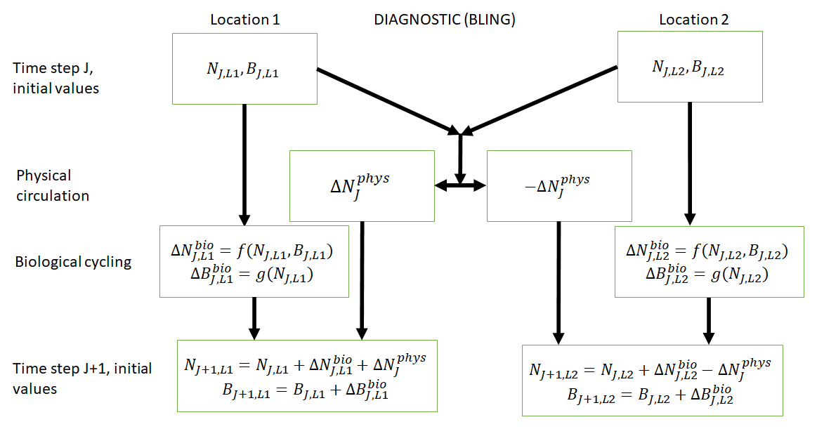
Figure 1 Conceptual diagram of how biogeochemical evolution is computed within an ESM using the BLING BC. The letters and abbreviations represent nutrients (N), phytoplankton biomass (B), the physical circulation component (phys), and the biological cycling component (bio). Each location has initial values for nutrients and biomass. These initial values are passed to the intrinsic biological relationships, which then feed into the g function in the biological cycling boxes that are then used to calculate the changes in nutrients and biomass due to biological cycling. The initial nutrient concentrations between the two locations result in a change in nutrients from physical transport, which is equal in magnitude and opposite in sign between the two boxes (physical circulation component). When the physical circulation and biological cycling portions are coupled together, the nutrients and biomass for the next time step are calculated.

2.3 Tracers of Phytoplankton with Allometric Zooplankton (TOPAZ)

TOPAZ is a prognostic biogeochemical model included in the Geophysical Fluid Dynamics Laboratory (GFDL) ESM2M (Dunne et al., 2013; Fig. 2). It includes a total of 30 tracers to model cycles such as nitrogen, phosphorus, iron, oxygen, carbon, and others (nutrients – N; Fig. 2). TOPAZ models three phytoplankton groups (small, large, and diazotrophic; biomass – B; Fig. 2) with irradiance limitation based on the equations of Geider et al. (1997). Additionally, phytoplankton loss and grazing as well as particle export are modeled using the same size-dependent formulation as those used in Eq. (2), though without imposing the quasi-equilibrium assumption that leads to Eq. (4). TOPAZ differs from BLING in its number of tracers (and associated limitations) and the allowance for advection–diffusion of nutrients and biomass ($\mathrm{\Delta }{B}_j^{\mathrm{phys}}$ in Fig. 2). This means that the loss rate of phytoplankton in TOPAZ is effectively a function of circulation as well the temperature- and biomass-dependent grazing rate, $\mathit{\lambda }{\left(\frac{B}{B_{\cdot }}\right)}^{\mathit{\alpha }}$. This will produce different biomasses in locations that have the same growth rates. Additionally, a key difference between BLING and TOPAZ is that the latter includes denitrification and nitrogen fixation. This then means (as suggested by Tyrrell, 1999) that the nitrogen is the proximate limiting nutrient, while phosphorus is the ultimate limiting nutrient; this is a distinction that is not made in BLING.

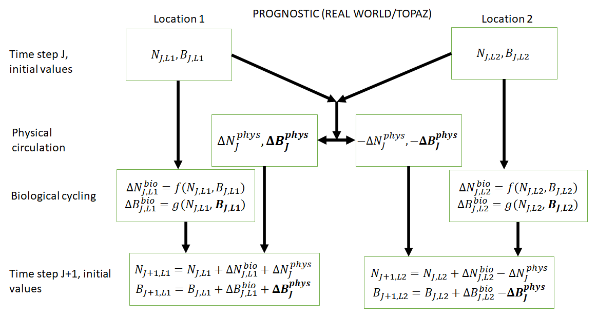
Figure 2 Conceptual diagram of how biogeochemical evolution is computed within an ESM using the prognostic TOPAZ BC. The letters and abbreviations represent nutrients (N), phytoplankton biomass (B), the physical circulation component (phys), and the biological cycling component (bio). This ESM differs from the one described in Fig. 1. In this prognostic model, the changes in biomass from the biological cycling component are a function of the nutrients and biomass rather than nutrients alone. Additionally, a change in biomass due to physical circulation is added.

3 Case descriptions

3.1 Case 1 – same ESM: identical biological equations, different physical circulations

The aim of Case 1 is to quantify the extent to which differences in physical circulations between model runs of the same ESM with identical intrinsic biological relationships could affect the apparent relationships found by NNEs. As stated in Sect. 2.1, we compare versions of GFDL ESM2Mc in which BLING is configured identically so we can be certain the differences are solely due to circulation changing the environmental conditions, and not the phytoplankton loss rates. Within GFDL ESM2Mc, the nominal resolution is 3^∘ longitudinally and 2^∘ latitudinally, while the vertical resolution has 28 levels. Model runs are initialized with observations and spun up for 1900 years. The final 100 years are used to generate a monthly climatology.

We use three configurations of GFDL ESM2Mc. The three model runs consist of a standard historical pre-industrial model spin-up (BLING – PI Control), a similar case to the first but in which the carbon dioxide concentration is 4 times higher (BLING – 4×CO₂), and a case similar to the historical spin-up except that the horizontal mixing parameter is 3 times higher (BLING – 3×Mixing). These model runs are described in greater detail in Gnanadesikan et al. (2013), Pradal and Gnanadesikan (2014), and Bahl et al. (2020). With the standard historical model essentially serving as a form of a “control”, the two remaining cases allow us to examine if changes in the physical circulation could result in changes to the apparent relationships.

The predictor variables for each model run are macronutrient (e.g., phosphate), micronutrient (e.g., dissolved iron), irradiance, and temperature. The target variables are small phytoplankton biomass and large phytoplankton biomass. One NNE is trained for each target variable of each model run for a total of six NNEs in Case 1 (three model runs and two target variables in each run). Details of the NNE training and the construction of the individual NNs making up each NNE can be found in Sect. 3.4.

3.2 Case 2 – same ESM: different diagnostic biological equations, nearly identical physical circulations

The purpose of Case 2 is to quantify the differences found by NNEs between the apparent relationships of model runs from the same ESM when the biological equations differ between runs, but the physical circulations are nearly identical.

As in Case 1, we use different configurations of ESM2Mc, but this time we keep the physical parameterizations constant and change constants within the BLING BC. We use two model runs: the standard historical pre-industrial model spin-up used in Case 1 (BLING – PI Control) and one with distributions similar to PI Control but different half-saturation coefficients (K_Fe and $K_{{\mathrm{PO}}_{\mathrm{4}}}$ in Eq. 3) for small and large phytoplankton (BLING – LgSm). Changing the half-saturation coefficients, which directly affects phytoplankton growth, is analogous to changing the biological equations. Relative to the PI Control, the half-saturation coefficients in LgSm are decreased by $\sqrt{\mathrm{3}}$ for small phytoplankton and increased by $\sqrt{\mathrm{3}}$ for large phytoplankton. While these changes produce differences in circulation and sea surface temperature (SST) via changing the absorption of shortwave radiation, these differences are small (R²=0.9949 for SST between the two model runs). The primary impact of these changes is to affect the distribution of nutrients, as increasing the half-saturation coefficients for large phytoplankton makes it harder for these phytoplankton to grow and efficiently export nutrients.

The predictor variables for the model runs of Case 2 are the same as those in Case 1 (macronutrient, micronutrient, irradiance, and temperature). Likewise, the target variables are also the same as those in Case 1 (small and large phytoplankton biomass). A total of four NNEs are trained for Case 2 (two model runs and two target variables).

3.3 Case 3 – different ESMs: prognostic vs. diagnostic biological equations, identical physical circulations

For Case 3, the goal is to examine whether the results from a diagnostic BC from Cases 1 and 2 still hold when a prognostic BC is used. Our goal is to examine any differences in apparent relationships, along with identifying challenges when comparing apparent relationships across more realistic ESMs. In this experiment, the BCs are governed by different biological equations but are run within the same physical model so that the temperatures and irradiance seen by the two BC codes are identical.

One of our model simulations uses a version of BLING as the BC, while the other uses TOPAZ. For the BLING model run, the iron concentrations are fixed at their climatological values since this formulation was previously used to develop a model for very high-resolution studies (miniBLING). We use this pair of simulations since the miniBLING code is run in an identical physical circulation to the TOPAZ model run, so the irradiance and temperature experienced by the two model ecosystems are identical. The ESM2M uses a 1^∘ latitude–longitude resolution with 50 vertical layers and the model is spun up for 2400 years. These simulations are described in more detail in Galbraith et al. (2015), which shows that BLING and miniBLING yield essentially identical predictions for carbon uptake and ocean deoxygenation under increased CO₂.

The predictor variables for Case 3 are limited to variables that are present in both ESMs: macronutrient, micronutrient, and irradiance. The target variable is total biomass. The biomass is not split into small and large phytoplankton biomass because the miniBLING output only contains total biomass. For consistency, the small and large phytoplankton biomass values in TOPAZ are combined to give total biomass. Two NNEs are trained for Case 3 (two ESM runs and one target variable).

3.4 Neural network ensembles (NNEs)

NNEs are an ensemble ML method. NNEs are comprised of a collection of individual neural networks (NNs) with the predictions of each NN averaged into a single prediction. This ensemble approach has been shown to outperform individual NNs and reduce the generalization error within a dataset (Hansen and Salamon, 1990) by turning individual “weak learners” into a single “strong learner.” Individual NNs can fit a nonlinear function to a dataset without assuming any prior knowledge of the system. For a more thorough discussion of NNs, please refer to Schmidhuber (2015). The basic structure of the NN approach that we use here is described in Appendix 1 of Scardi (1996).

We use NNEs for several reasons.

1. The ensemble approach of NNEs allows us to view the uncertainty in any given prediction based on the individual predictions of each NN.

2. NNEs possess some capability of extrapolating outside the range of the data on which they are trained (Holder and Gnanadesikan, 2021).

3. As recently shown in Holder and Gnanadesikan (2021), NNEs were able to more closely reproduce the underlying intrinsic relationships compared to random forests, mainly because of their ability to extrapolate.

The structure of the individual NNs is consistent between the three cases, with each NN containing 25 nodes in the hidden layer with a hyperbolic tangent sigmoid activation function and 1 node in the output layer with a linear activation function. We demonstrated in previous work that the NNE predictions were not greatly improved with the addition of a second hidden layer or with hidden layer node quantities greater than 25 (Holder and Gnanadesikan, 2021). Additionally, the activation function of the hidden layer nodes did not see a substantial increase in performance either as long as a nonlinear function was used (Holder and Gnanadesikan, 2021). The settings specified here allow for reasonable training times while maintaining high performance metrics relative to the other formulations tested in our previous work (Holder and Gnanadesikan, 2021). For more detailed information, see Appendix B2 in Holder and Gnanadesikan (2021).

Table 1 Summary of each case, which includes information on the predictor variables, the target variables, the ESMs, the model runs, the biological specifications, and the physical circulation specifications.

The difference between each case is in the number of input nodes: Cases 1 and 2 each contain four input nodes (one for each predictor), and Case 3 has three input nodes. The predicted concentration of each target variable (second column of Table 1) in individual NNs can be thought of as a function of the respective predictors (first column of Table 1). For example, one NN of the NNE for the small phytoplankton biomass target variable in Case 1 would have the following structure.

1. The four predictor variables for Case 1 (first column of Table 1) correspond to the four nodes in the input layer of the NN.

2. Each of the four input nodes is connected by weights to each of the 25 nodes in the hidden layer. Additionally, a bias term is connected to each of the hidden nodes.

3. Each of the nodes in the hidden layer is connected by weights to the single node in the output layer, which, for this instance, would correspond to the target variable of small phytoplankton biomass. As with the hidden layer, a bias term is connected to the single output node.

The training of each NN is carried out using the “feedforwardnet” function in MATLAB (MATLAB, 2019). For each trained NN, the “feedforwardnet” function is provided with the training dataset, which it then automatically separates into training, validation, and testing subsets, with 70 % of the observations from the training dataset going to the training subset, 15 % to the validation subset, and 15 % to the testing subset. The training stops when the error between the predictions and observations increases for six consecutive epochs.

Separate NNEs are trained for each response variable in each model run, which equates to six NNEs (two target variables, three simulations) in Case 1, four NNEs in Case 2, and two NNEs in Case 3. For consistency, the same framework and settings are used for the construction of the NNEs, with each one consisting of 25 individuals NNs.

Each variable is also scaled between −1 and 1 relative to each variable's maximum and minimum:

$$\begin{array}{}\text{(5)}& {\displaystyle }{V}_{\mathrm{S}}={\displaystyle \frac{{max}_{\mathrm{S}}-{min}_{\mathrm{S}}}{{max}_{\mathrm{U}}-min{}_{\mathrm{U}}}}\left(V_{\mathrm{U}}-{\min }_{\mathrm{U}}\right)+{\min }_{\mathrm{S}},\end{array}$$

where V is the value of a variable being scaled, S (subscript) is the scaled value, and U (subscript) is the unscaled value. This scaling puts the predictor values in the same range, so more weight is not given to variables with larger ranges. Additionally, this step decreases the training time of the NNs so that no values are too close to the limits of the hyperbolic tangent sigmoid activation function. The variables and predictions are then scaled back to their original values for analysis and presentation of the results (Eq. 6). The letter representations in Eq. (6) are the same as those in Eq. (5).

$$\begin{array}{}\text{(6)}& {\displaystyle }{V}_{\mathrm{U}}={\displaystyle \frac{{max}_{\mathrm{U}}-{min}_{\mathrm{U}}}{{max}_{\mathrm{S}}-min{}_{\mathrm{S}}}}\left(V_{\mathrm{S}}-{\min }_{\mathrm{S}}\right)+{\min }_{\mathrm{U}}\end{array}$$

When using ML, it is possible to produce overly complex relationships that “overfit” the data. This provides a good match for the data on which an ML model is trained but leads to poor predictions when new data are presented to the model. This can be avoided by splitting a dataset into training and testing subsets. For this paper, this means each NNE is trained using only the observations in the training subset and tested on the observations from the testing subset. The data from each model run are randomly split into training and testing subsets with 60 % of the observations from a dataset going to the training subset and the other 40 % going to the testing subset. The observations set aside in the testing subset are ones that the NNEs never see during their training phase. This provides a way to evaluate each trained NNE and its generalizability. If performance metrics of a trained NNE are similar between the training and testing subsets, it suggests that the variance of the dataset is well captured in the training phase and the NNE is generalizable to the entire dataset.

To assess the performance of each NNE, we calculate the standard R² values and root mean squared error (RMSE) by comparing the monthly biomass predictions from each NNE to the “true” monthly biomass values of the model runs within the respective training and testing subsets.

The NNEs in each case and matching size class are also asked to make predictions on the testing subsets of the other model runs. For example, in Case 1 the NNE trained on the small phytoplankton of PI Control is asked to make predictions for small phytoplankton of 4×CO₂ using the values of the predictors from the testing subset of the 4×CO₂ model run. These results are then compared to the actual values of the target variable to calculate the RMSE. This RMSE is then used to calculate the percent increase or decrease in error when compared against the RMSE calculated from a point-by-point comparison of each model run against the others. The purpose of this is to provide another metric for testing if the NNEs are finding common apparent relationships across model runs. If an NNE trained on one model run is able to predict the outcomes of the other model runs with errors that are similar in magnitude to the NNEs that were trained on those runs, it would suggest that the NNEs are finding similar apparent relationships between the model runs. On the other hand, if it shows an increase in RMSE, it suggests that the apparent relationships between the model runs are different in biologically important ways.

To view the apparent relationships found by the NNEs, we conduct sensitivity analyses in which we present each NNE with a unique set of values for the predictors. Compared to spatiotemporal distributions and time series, sensitivity analyses allow for the visualization of relationships between predictor and target variables. In each sensitivity analysis, one predictor is varied across its minimum and maximum range, while the other variables are held at a specified value, such as each variable's 25th percentile. This is repeated for the 50th and 75th percentile values of each variable as well. This allows us to visualize how the biomass predictions change across one variable's range when the other variables are held at a specified value. An example of this is varying the macronutrient concentration while holding the micronutrient, irradiance, and temperature variables at their 25th or 75th percentile values. This allows us to see how the macronutrient concentration affects biomass when other nutrients are low or high, respectively.

4 Results and discussion

4.1 Case 1 – same ESM: identical biological equations, different physical circulations

In Case 1, our objective is to quantify the extent to which differences in physical circulation might affect the apparent relationships found by NNEs when the intrinsic biological relationships remain the same between the model runs and the physical circulation parameters differ. It is uncertain whether changing the circulation would lead to new patterns of co-limitation (i.e., different apparent relationships) or whether the physical circulation would simply act to change the location at which combinations of irradiance and nutrients are found (i.e., same apparent relationships).

Our results support the latter outcome that the locations of particular environments are simply being shuffled around. The sensitivity analysis shows that each NNE finds similar apparent relationships between biomass and each of the predictors for the respective size classes, insofar as each line falls within the standard deviation of the others (Figs. 3 and 4). For example, the standard deviation (gray region) around the predicted apparent relationships for the large phytoplankton (dashed lines) all overlap one another (Fig. 3). The same is seen for the predicted apparent relationships for the small phytoplankton (Fig. 4). Additionally, we are confident in the apparent relationships since each NNE acquires high performance metrics in both the training and testing subsets (highest RMSE $=\mathrm{3.11}\times {\mathrm{10}}^{-\mathrm{9}}$ mol P kg⁻¹; Table 2) relative to the mean value of the total biomass ($\mathrm{1.24}\times {\mathrm{10}}^{-\mathrm{8}}$ mol P kg⁻¹).

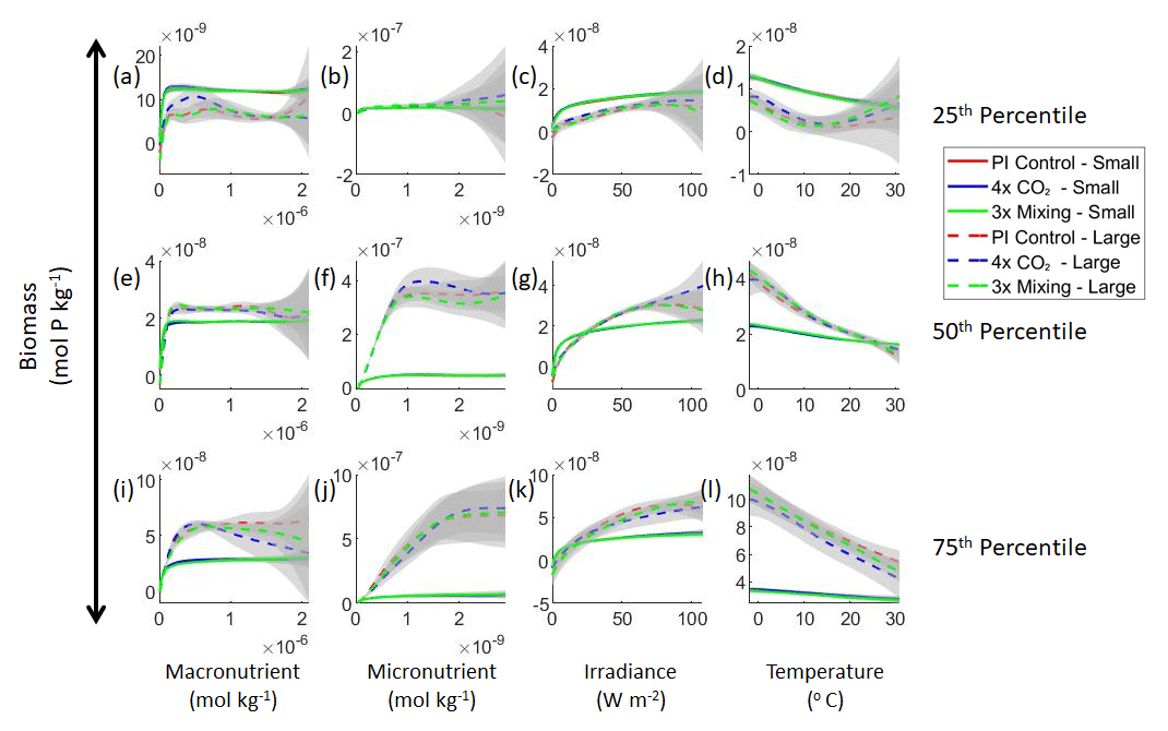
Figure 3 Sensitivity analysis plots for the small and large phytoplankton of Case 1. Each line is the prediction for the NNE (i.e., the average prediction of 25 NNs) specific to each model run, and the color of each line represents the model run (PI Control – red; 4×CO₂ – blue; 3×Mixing – green). The solid lines correspond to the NNE predictions for small phytoplankton and the dashed lines to the NNE predictions for large phytoplankton. The gray region around each line shows 1 standard deviation in the predictions of the individual NNs that make up each NNE (e.g., the gray region around the solid red curves shows the standard deviation in the predictions of the 25 NNs that make up that particular NNE). The rows correspond to the percentile value at which the other predictor variables are held constant (e.g., panel a varies the macronutrient across its min–max range and holds the micronutrient, irradiance, and temperature at their respective 25th percentile values). Columns show the x-axis variables as they vary between their min–max range. The y axis in all panels is the biomass concentration. Note that the biomass scale changes with each panel.

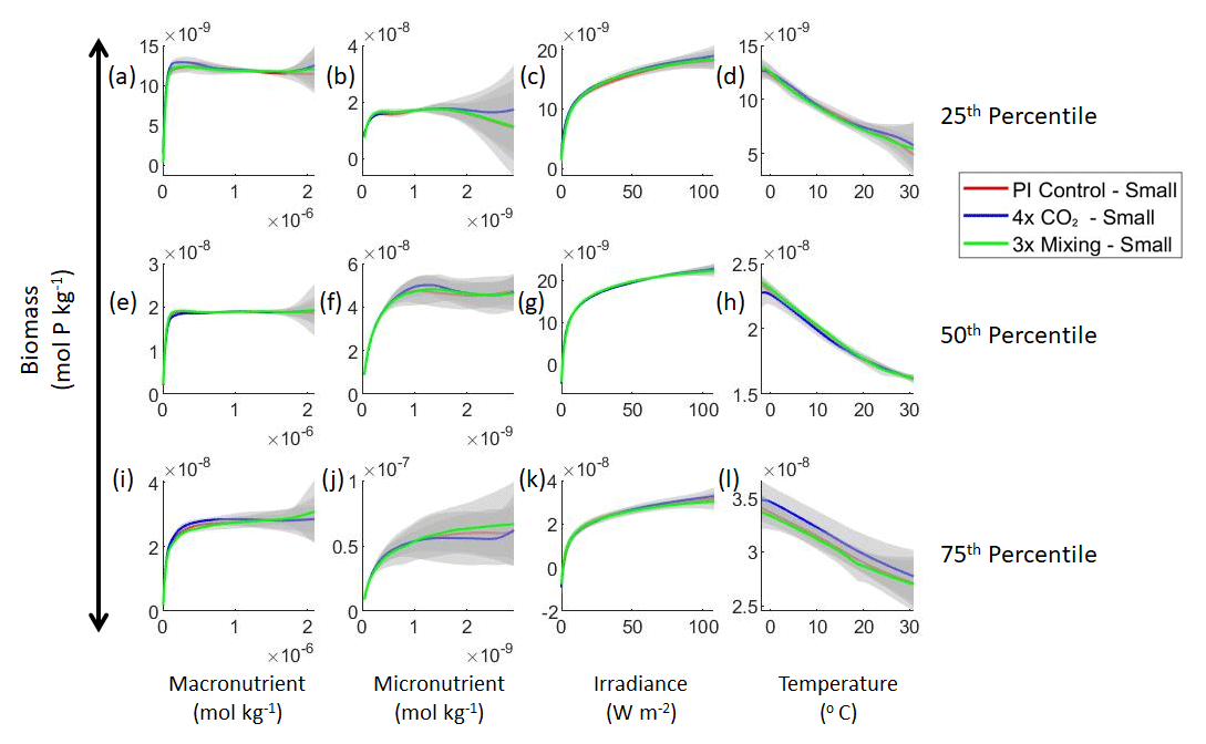
Figure 4 Sensitivity analysis plots for the small phytoplankton of Case 1. This figure is provided to allow for examination of the apparent relationships for the small phytoplankton, since the large phytoplankton apparent relationships made it difficult to see those for the small phytoplankton in Fig. 3. Each line is the prediction for the NNE (i.e., the average prediction of 25 NNs) specific to each model run, and the color of each line represents the model run (PI Control – red; 4×CO₂ – blue; 3×Mixing – green). The gray region around each line shows 1 standard deviation in the predictions of the individual NNs that make up each NNE (e.g., the gray region around the solid red curves shows the standard deviation in the predictions of the 25 NNs that make up that particular NNE). The rows correspond to the percentile value at which the other predictor variables were held constant (e.g., panel a varies the macronutrient across its min–max range and holds the micronutrient, irradiance, and temperature at their respective 25th percentile values). Columns show the x-axis variables as they vary between their min–max range. The y axis in all panels is the biomass concentration. Note that the biomass scale changes with each panel.

Table 2 The performance metrics for the training and testing subsets for the trained NNEs from each case separated into their respective size classes and ESM and/or model runs.

This result can be better understood by considering the conceptual diagram of how the diagnostic BC BLING works within an ESM (Fig. 1). For each time step, nutrients are calculated as a function of three terms: the initial nutrients, the change in nutrients from biology, and the change in nutrients from physical circulation. In contrast, the biomass is only a function of two terms: the initial biomass values and the change in biomass due to biological cycling. Thus, biomass is not directly affected by changes in the physical circulation. Additionally, this means that when given information on the biological predictors but not the physical parameters, the NNEs are able to identify the apparent relationships quite well. Although it would seem obvious from Fig. 1 that the biomass is not directly affected by changes in the physical circulation, we were unsure whether indirect impacts of such changes (changing patterns of co-limitation or temporal variability) would affect the results. Our results indicate that such indirect effects were absent or, at most, minor.

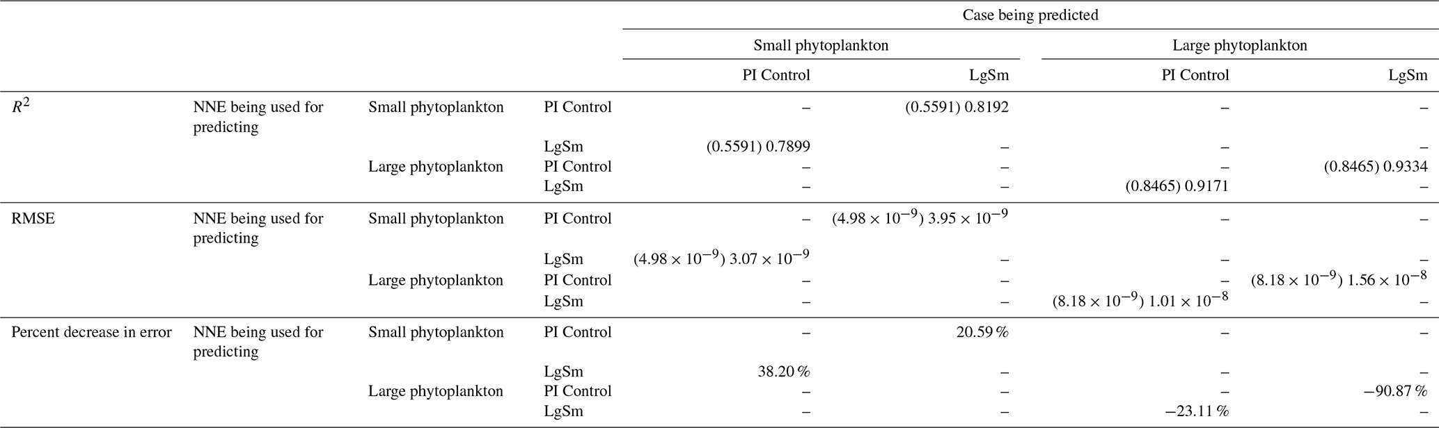
That similar apparent relationships are found between the model runs is further supported when we task each trained NNE with making predictions on the testing subsets of the other model runs for the same size class. For example, the NNE trained on the PI Control for small phytoplankton can be tasked with making predictions for the small phytoplankton biomass of 4×CO₂ and 3×Mixing using the predictor values from their testing subsets. This test allows for the evaluation of the robustness of the relationships that each NNE finds. If the NNEs are finding different relationships between the model runs, the NNE from one model run will likely perform poorly when predicting the other model runs. Our results show that the NNEs perform well when applied to the other model runs (highest RMSE = $\mathrm{3.74}\times {\mathrm{10}}^{-\mathrm{9}}$ mol P kg⁻¹; Table 3) relative to the average value of total biomass ($\mathrm{1.24}\times {\mathrm{10}}^{-\mathrm{8}}$ mol P kg⁻¹). Given that these values are close to the performance metrics of their original datasets (Table 2 vs. Table 3), it seems logical to say that this is because they are finding the same relationships.

Table 3 The performance metrics for the NNEs being used to predict the outcome of the other model runs for the same size class of Case 1. In the top half of the table, the R² and RMSE are listed. The values in parentheses are the values from comparing the respective cases against one another (these are the same values listed in the respective scatter plots in Fig. 5 and 6). The values outside the parentheses are the values from using the trained NNE of the model listed in the row to predict the outcome of the model run in the column (e.g., the NNE trained on 4×CO₂ was used to predict the PI Control outcome using the predictor values of PI Control; these values were compared against the actual values of the PI Control to compute the RMSE of $\mathrm{7.15}\times {\mathrm{10}}^{-\mathrm{10}}$). In the bottom half of the table is the percent decrease in RMSE from the number listed inside the parentheses to the RMSE outside the parentheses.

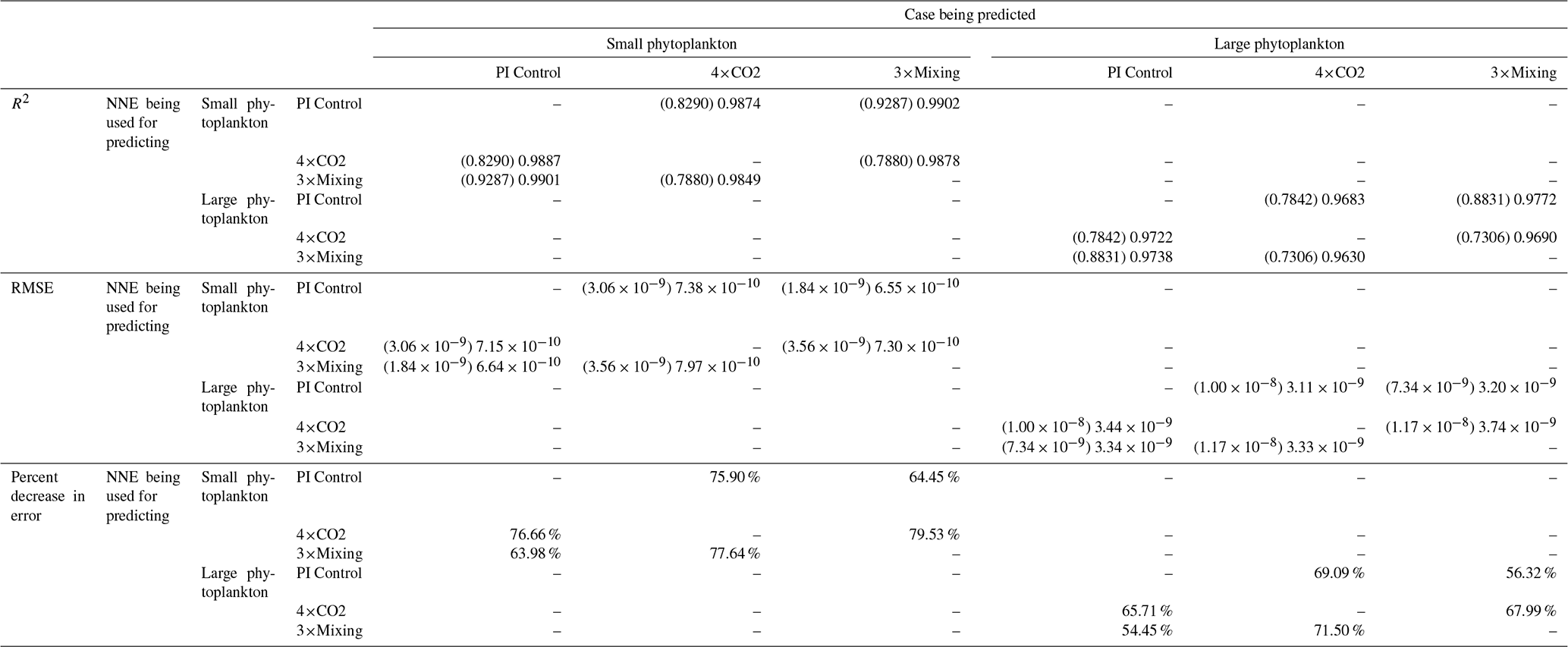
Additionally, using the NNEs to predict the other runs leads to decreases in error relative to the error from comparing each run against the others. For example, the initial point-by-point comparison of 4×CO₂ and PI Control for small phytoplankton (Fig. 5d) shows an RMSE of $\mathrm{3.06}\times {\mathrm{10}}^{-\mathrm{9}}$ mol P kg⁻¹, while using the NNEs from each model run to predict the other saw the RMSE go down with a reduction in error of about 76 % (Table 3). This reduction of error is consistent across the other model runs and size classes with error reductions varying from 54 %–79 % (Table 3). This implies the NNEs applied to the other runs are better able to predict the outcome than the point-by-point analysis, once again reinforcing our previous result.

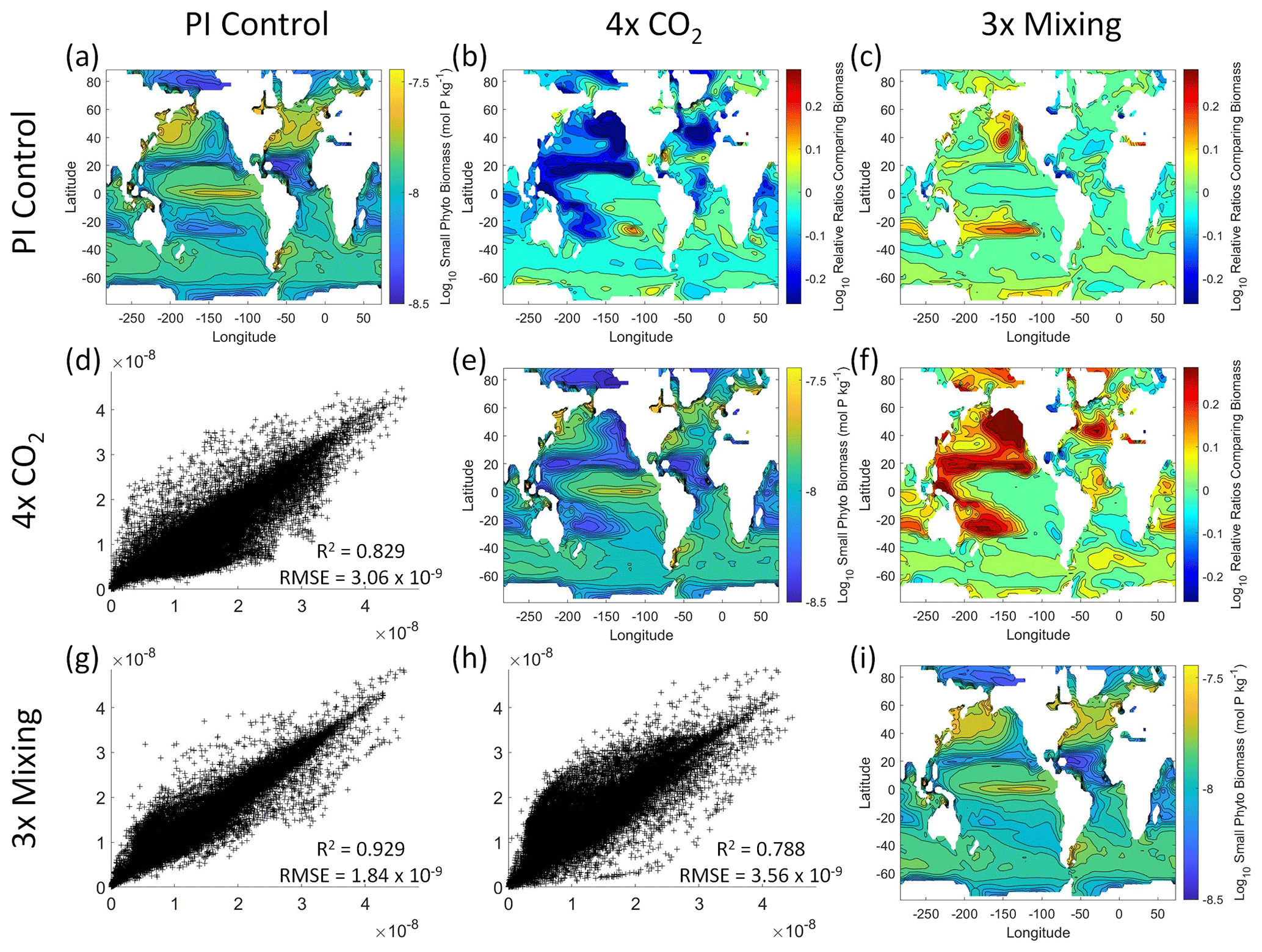
Figure 5 Comparison of the model runs for small phytoplankton biomass in Case 1. The units for biomass in all panels are mol P kg⁻¹. The panels show point-by-point scatter plots comparing the model runs against one another (d, g, h), yearly averaged log₁₀ biomass plots for each model run (a, e, i), and the log₁₀ relative ratios comparing the yearly averaged contour plots of the model runs (b, c, f). The x axis and y axis of the scatter plots (d, g, h) correspond to the horizonal and vertical model run labels, respectively (e.g., panel d shows PI Control on the x axis and 4×CO₂ on the y axis). The yearly averaged log₁₀ contour plots (a, e, i) correspond to the matching horizontal and vertical model run labels (e.g., panel a shows the yearly averaged log₁₀ biomass of PI Control). The log₁₀ relative ratios (b, c, f) were calculated as the model run listed on the horizontal axis divided by the model run listed on the vertical axis (e.g., panel b shows 4×CO₂ divided PI Control).

That the NNEs from one model run are able to reproduce the results from the other model runs is not simply due to the models producing similar spatiotemporal patterns. To ensure that distinct differences between the model runs are present, we compare each model run against the others (Figs. 5 and 6). Differences in the biomass values between the three model runs are evident (Figs. 5 and 6). First, we compare each model run against the others in a point-by-point analysis and observe that different biomasses are occurring at the same spatiotemporal locations (Figs. 5 and 6d, g, h). For example, in the small phytoplankton scatter plot for PI Control vs. 4×CO₂, PI Control shows a tendency of having biomass values higher than 4×CO₂ across most locations (Fig. 5d). Additionally, we look at the contour plots and log₁₀ relative ratios using the yearly averaged biomass for each case (Figs. 5 and 6a–c, e, f, i). Specific large differences that we note are higher biomass in the Pacific and North Atlantic in PI Control and 3×Mixing relative to 4×CO₂ (Figs. 5 and 6b, f) and the highest biomass occurring in 3×Mixing in the subtropical regions of the Pacific (Figs. 5 and 6c). Similar patterns are observed in the large phytoplankton as well (Fig. 6). These differences between the model runs are relatively large (exceeding a factor of 3 in some locations) and allow us to dismiss the possibility that the similar apparent relationships are only due to strong similarities between the model runs.

Figure 6 Comparison of the model runs for large phytoplankton biomass in Case 1. The units for biomass in all panels are mol P kg⁻¹. The panels show point-by-point scatter plots comparing the model runs against one another (d, g, h), yearly averaged log₁₀ biomass plots for each model run (a, e, i), and the log₁₀ relative ratios comparing the yearly averaged contour plots of the model runs (b, c, f). The x axis and y axis of the scatter plots (d, g, h) correspond to the horizonal and vertical model run labels, respectively (e.g., panel d shows PI Control on the x axis and 4×CO₂ on the y axis). The yearly averaged log₁₀ contour plots (a, e, i) correspond to the matching horizontal and vertical model run labels (e.g., panel a shows the yearly averaged log₁₀ biomass of PI Control). The log₁₀ relative ratios (b, c, f) were calculated as the model run listed on the horizontal axis divided by the model run listed on the vertical axis (e.g., panel b shows 4×CO₂ divided PI Control).

Although the sensitivity analysis allows us to see that the apparent relationships were the same for each size class, it also allows us to see how the two size classes react differently to the same conditions. Most notably, the large phytoplankton seem to be very sensitive to the micronutrient compared to the small phytoplankton (Fig. 3; closer view of small phytoplankton in Fig. 4). When the other predictors are held at their 75th percentile values (high macronutrient, high irradiance, and warm temperature), the large phytoplankton reach biomass values almost an order of magnitude higher than the small phytoplankton (Figs. 3 and 4j). This is what would be expected given the cubic relationship of large phytoplankton with growth rate. Another interesting relationship is the stark asymptotes in both size classes of the macronutrient plots, suggesting limitations by other nutrients, likely the micronutrient (Fig. 3a, e, i). One unexpected relationship is the decreasing biomass with increasing temperature in both size classes (Fig. 3d, h, l). This could be a result of warmer regions having fewer available nutrients or because of the temperature-dependent chlorophyll-to-carbon (Chl:C) ratios (Geider et al., 1997), which would lead to phytoplankton needing higher irradiance in warmer waters.

Relative to our main objective in Case 1 to quantify the extent to which differences in physical circulation affect the apparent relationships, our results indicate that the different physical circulations do not produce differences in the apparent relationships found by NNEs. When the biological equations remain the same, changing the physical parameters simply changes where combinations of nutrients and irradiance occur. The NNEs can find the same apparent relationships between the model runs when the equations and constants governing those runs are identical, even if the inputs differ. In contrast to changes in nutrients, changes in biomass in the BLING ESM are not a function of the physical circulation.

4.2 Case 2 – same ESM: different diagnostic biological equations, nearly identical physical circulations

In Case 1, it is clear from our results that when the biological cycling is identical between model runs, the NNEs find the same apparent relationships because the biomass is not a function of the physical circulation. Since the biomass is clearly a function of the biological equations, it would be reasonable to assume that the apparent relationships could be different between model runs that are governed by different biological equations. So, for Case 2, the objective is to quantify the extent to which NNEs can detect differences in the apparent relationships when the intrinsic biological relationships between model runs are different, while maintaining similar physical circulations and still using a diagnostic model which guarantees that identical nutrient, irradiance, and temperature at two different points will produce identical biomass.

Our results show that NNEs can differentiate the apparent relationships between model runs when the biological equations differ. The sensitivity analysis for Case 2 shows that different apparent relationships are found between model runs and within the same size classes relative to the non-overlapping gray standard deviation regions around each line (Figs. 7 and 8). Additionally, we can be fairly confident in these predictions given the high performance metrics in both the training and testing subsets (highest RMSE $=\mathrm{3.11}\times {\mathrm{10}}^{-\mathrm{9}}$ mol P kg⁻¹ – Table 2 – vs. the average total biomass of $\mathrm{1.36}\times {\mathrm{10}}^{-\mathrm{8}}$ mol P kg⁻¹).

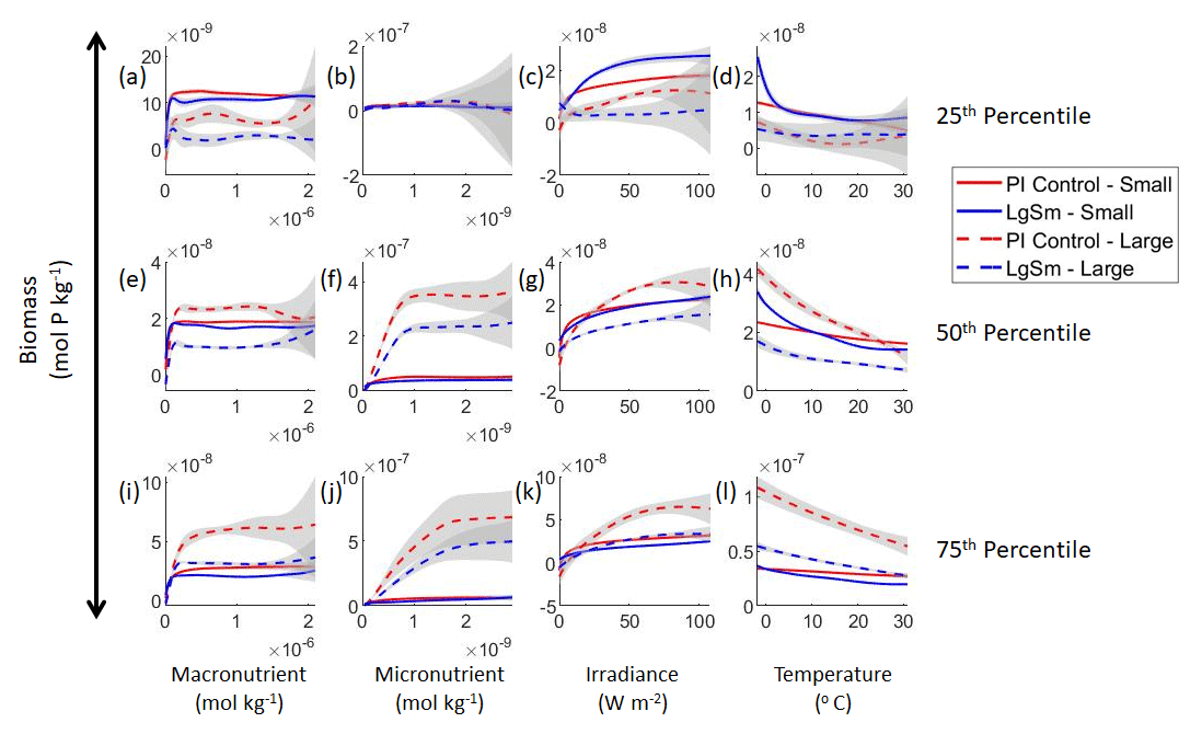
Figure 7 Sensitivity analysis plots for the small and large phytoplankton of Case 2. Each line is the prediction for the NNE (i.e., the average prediction of 25 NNs) specific to each model run, and the color of each line represents the model run (PI Control – red; LgSm – blue). The solid lines correspond to the small phytoplankton and the dashed lines to the large phytoplankton. The gray region around each line shows 1 standard deviation in the predictions of the individual NNs that make up each NNE (e.g., the gray region around the solid red curves shows the standard deviation in the predictions of the 25 NNs that make up that particular NNE). The rows correspond to the percentile value at which the other predictor variables were held constant (e.g., panel a varies the macronutrient across its min–max range and holds the micronutrient, irradiance, and temperature at their respective 25th percentile values). Columns show the x-axis variables as they vary between their min–max range. The y axis in all panels is the biomass concentration. Note that the biomass scale changes with each panel.

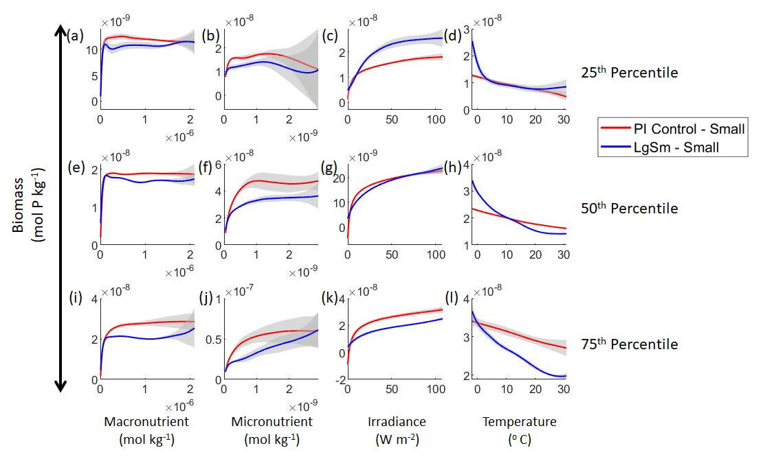
Figure 8 Sensitivity analysis plots for the small phytoplankton of Case 2. This figure is provided to allow for examination of the apparent relationships for the small phytoplankton, since the large phytoplankton apparent relationships made it difficult to see those for the small phytoplankton in Fig. 7. Each line is the prediction for the NNE (i.e., the average prediction of 25 NNs) specific to each model run, and the color of each line represents the model run (PI Control – red; LgSm – blue). The gray region around each line shows 1 standard deviation in the predictions of the individual NNs that make up each NNE (e.g., the gray region around the solid red curves shows the standard deviation in the predictions of the 25 NNs that make up that particular NNE). The rows correspond to the percentile value at which the other predictor variables were held constant (e.g., panel a varies the macronutrient across its min–max range and holds the micronutrient, irradiance, and temperature at their respective 25th percentile values). Columns show the x-axis variables as they vary between their min–max range. The y axis in all panels is the biomass concentration. Note that the biomass scale changes with each panel.

This result of different relationships, when the model runs are governed by different biological equations, reinforces what we found in Case 1. Changing the biological equations can be likened to changing how the nutrients affect the phytoplankton biomass (the function $g\left(N_{J,L\mathrm{1},L\mathrm{2}}\right)$ in Fig. 1). While it might seem obvious that changing the biological equations will change the biomass values, it remains unclear whether NNEs would be able to pick out these differences in the apparent relationships.

We want to ensure there are noticeable differences between the model runs (Figs. 9 and 10). We did this in Case 1 to ensure that the similar apparent relationships found by the NNEs were not simply because of similarities in the model output. In Case 2, the difference in model outputs serves to reinforce the different apparent relationships found by the NNEs. In the point-by-point comparison, the large phytoplankton show more agreement between model runs (Fig. 10c) than the small phytoplankton (Fig. 9c). However, when we examine the contour and log₁₀ relative ratios (Figs. 9 and 10a, b, d), it is evident that large, systematic, spatially coherent differences exist between the model runs. Both the small and large phytoplankton show higher concentrations in the LgSm model run compared to PI Control for the subtropical and polar regions of the Pacific and Indian oceans, along with higher concentrations in the equatorial Atlantic (Figs. 9 and 10).

Figure 9 Comparison of the model runs for small phytoplankton biomass in Case 2. The units for biomass in all panels are mol P kg⁻¹. The panels show point-by-point scatter plots comparing the model runs against one another (c), yearly averaged log₁₀ biomass plots for each model run (a, d), and the log₁₀ relative ratios comparing the yearly averaged contour plots of the model runs (b). The x axis and y axis of the scatter plots (c) correspond to the horizonal and vertical model run labels, respectively (e.g., panel c shows PI Control on the x axis and LgSm on the y axis). The yearly averaged log₁₀ contour plots (a, d) correspond to the matching horizontal and vertical model run labels (e.g., panel a shows the yearly averaged log₁₀ biomass of PI Control). The log₁₀ relative ratios (b) were calculated as the model run listed on the horizontal axis divided by the model run listed on the vertical axis (e.g., panel b shows LgSm divided PI Control).

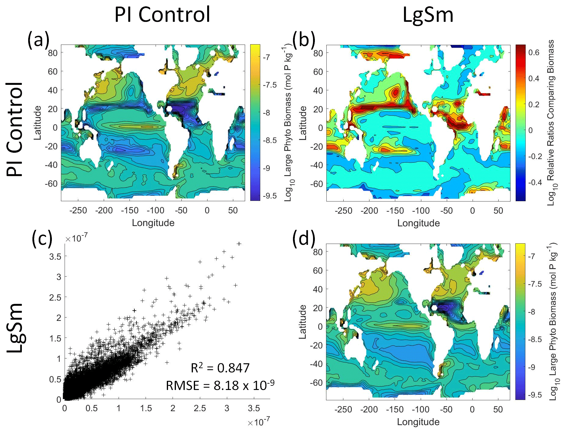
Figure 10 Comparison of the model runs for large phytoplankton biomass in Case 2. The units for biomass in all panels are mol P kg⁻¹. The panels show point-by-point scatter plots comparing the model runs against one another (c), yearly averaged log₁₀ biomass plots for each model run (a, d), and the log₁₀ relative ratios comparing the yearly averaged contour plots of the model runs (b). The x axis and y axis of the scatter plots (c) correspond to the horizonal and vertical model run labels, respectively (e.g., panel c shows PI Control on the x axis and LgSm on the y axis). The yearly averaged log₁₀ contour plots (a, d) correspond to the matching horizontal and vertical model run labels (e.g., panel a shows the yearly averaged log₁₀ biomass of PI Control). The log₁₀ relative ratios (b) were calculated as the model run listed on the horizontal axis divided by the model run listed on the vertical axis (e.g., panel b shows LgSm divided PI Control).

Although the gray regions in Figs. 7 and 8 overlap toward the higher concentrations of each predictor, this is likely due to the lack of observations in the training data meeting those criteria, without which the NNEs cannot be constrained. For example, in Fig. 7j, the apparent relationships of the large phytoplankton overlap past about $\mathrm{5}\times {\mathrm{10}}^{-\mathrm{10}}$ mol kg⁻¹ of the micronutrient because there are no observations in the training data that are greater than $\mathrm{5}\times {\mathrm{10}}^{-\mathrm{10}}$ mol kg⁻¹ of the micronutrient while simultaneously being at the 75th percentile level of the macronutrient, irradiance, and temperature (data not shown). Without observations to constrain them, the NNEs cannot be constrained and are therefore less certain about the extrapolated relationships in those regions, which leads to higher uncertainty and overlapping standard deviations.

As in Case 1, our result is supported by the additional test in which the NNEs trained on one model run are tasked with making predictions on the other. Had the NNEs found similar apparent relationships, the reductions in error would have been of similar magnitude as those in Case 1 (Table 3 vs. Table 4). For this second case, we see that there are only modest decreases in RMSE for the small phytoplankton and increases in RMSE for large phytoplankton (Table 4). For example, relative to the RMSE of the point-by-point comparison, the RMSE decreases about 21 % when LgSm makes predictions on PI Control for the small phytoplankton (Table 4). Additionally, it is observed that even though the RMSE increases in the large phytoplankton, the R² values improve in the cross-model comparison compared to the point-by-point comparison (0.92–0.93 vs. 0.85; Table 4). This suggests that the NNEs improve the simulation in terms of the overall pattern but not the magnitude. These results make sense since the apparent relationships of the small phytoplankton show greater similarities than the apparent relationships of the large phytoplankton (Fig. 7).

Table 4 The performance metrics for the NNEs being used to predict the outcome of the other model runs for the same size class of Case 2. In the top half of the table, the R² and RMSE are listed. The values in parentheses are the values from comparing the respective cases against one another (these are the same values listed in the respective scatter plots in Figs. 9 and 10). The values outside the parentheses are the values from using the trained NNE of the model listed in the row to predict the outcome of the model run in the column (e.g., the NNE trained on LgSm was used to predict the PI Control outcome using the predictor values of PI Control; these values were compared against the actual values of the PI Control to compute the RMSE of $\mathrm{3.07}\times {\mathrm{10}}^{-\mathrm{9}}$). In the bottom half of the table is the percent decrease in RMSE from the number listed inside the parentheses to the RMSE outside the parentheses (a negative percent means that the error increased).

With respect to the apparent relationships that the NNEs uncover, the large phytoplankton once again appear to be more sensitive to the micronutrient concentrations compared to the small phytoplankton (Fig. 7b, f, j). Both size classes show asymptotes around the same concentrations for the macronutrient, albeit at different biomass values (Fig. 7a, e, i). As with Case 1, the decreasing biomass with increasing temperature is an unexpected relationship (Fig. 7d, h, l), which might be explained by the temperature-dependent Chl:C ratios causing phytoplankton in warmer regions to need higher irradiance.

As previously stated, our main objective with Case 2 is to quantify the extent to which NNEs can detect differences in the apparent relationships when the physical conditions between model runs are identical and the biological relationships differ. With the biomass being a function of changes in biomass from biology (i.e., the equations governing how nutrients affect biomass), it is unsurprising that different biological equations produce differences in biomass. What was unclear was whether NNEs would be able to highlight these differences in the apparent relationships. Our results indicate that NNEs can find noticeable differences in the apparent relationships, insofar as the standard deviation regions of the sensitivity analysis curves do not overlap.

4.3 Case 3 – different ESMs: prognostic vs. diagnostic biological equations, identical physical circulations

From Cases 1 and 2, we learn from our results that NNEs are capable of discerning differences in apparent relationships between model runs of the same ESM. For Case 3, we apply these principles to different ESMs to quantify the differences in the apparent relationships and highlight challenges that arise in comparing relationships between ESMs. The model runs of Cases 1 and 2 using BLING as a BC afford us the opportunity to test a “best-case” scenario for predicting biomass from nutrients and irradiance because of the tight coupling of growth rate and biomass (i.e., knowing the growth rate means we know the biomass). In Case 3, the ESMs have different biogeochemical codes (i.e., different biological equations) and identical physical circulations. One ESM (ESM2Mo with miniBLING as BC, referred to as miniBLING) is comparable to the BLING formulation in that the growth rate is tightly coupled with the biomass. However, the other ESM (ESM2Mo with TOPAZ as BC, referred to as TOPAZ) does not have as tight of a coupling. The TOPAZ simulation allows biomass to be advected and diffused in the same way as nutrients, effectively making biomass a function of nutrients and physical circulation, which is more typical of ESMs and likely true in the real ocean as well.

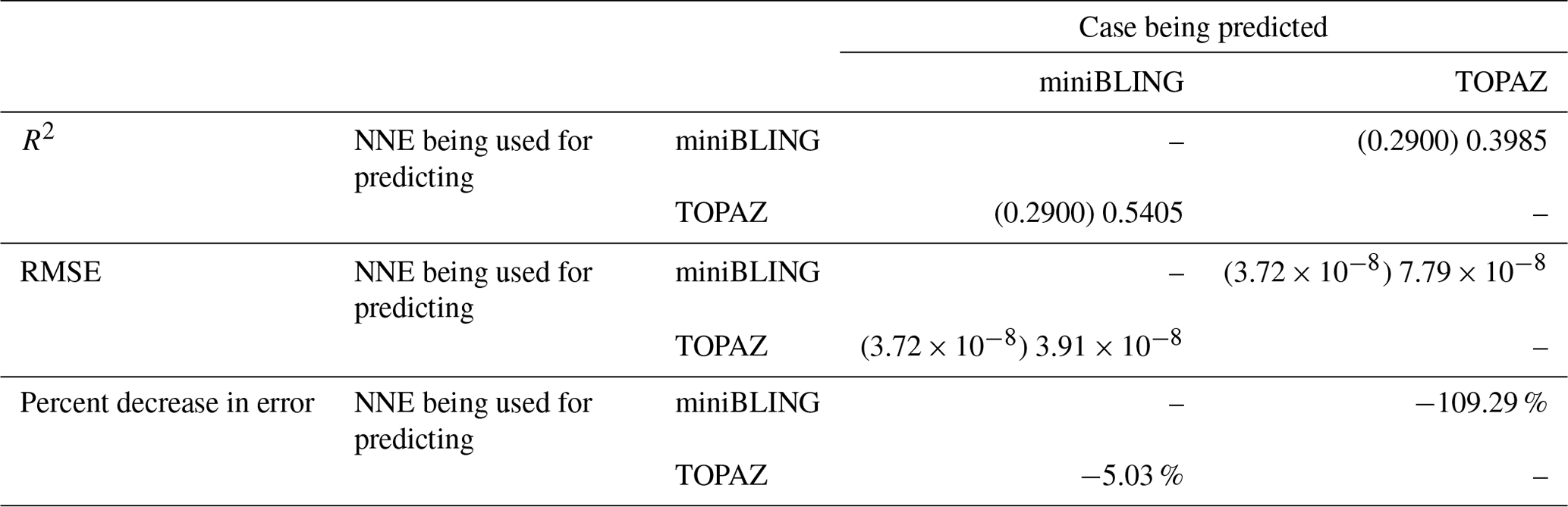
Our results indicate that the phytoplankton in the two ESMs react differently to the same conditions. It should be noted that total phytoplankton biomass is used for Case 3 rather than splitting the biomass into large and small because phytoplankton output by the miniBLING BC is not differentiated into size classes. The sensitivity analysis shows that the miniBLING simulation produces higher biomass concentrations than the TOPAZ simulation under the same conditions (Fig. 11), except at lower concentrations of nutrients at which they seem to react similarly (Fig. 11a, b, c). This is not entirely unexpected since the biomass values in the miniBLING simulation are generally much higher than those in the TOPAZ simulation, as can be seen in the point-by-point comparison (Fig. 12c). However, not all the biomass values in the miniBLING simulation are larger than those in the TOPAZ simulation. The subtropical Atlantic regions and northern subtropical Pacific have higher yearly averaged biomass values in the TOPAZ simulation compared to the miniBLING simulation (Fig. 12a, b, d). As with Case 2, the additional test of asking the NNEs trained on the output of one ESM to predict the output from the other ESM reinforces the result that different apparent relationships are found from an increase in error for both ESMs (Table 5).

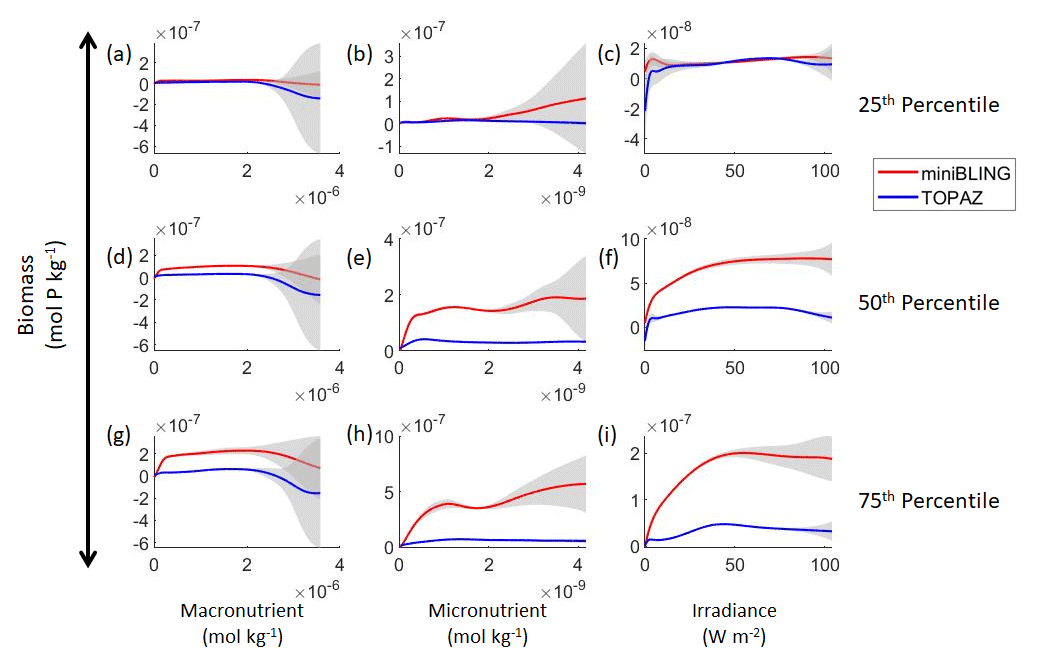
Figure 11 Sensitivity analysis plots for phytoplankton biomass for Case 3. Each line is the prediction for the NNE (i.e., the average prediction of 25 NNs) specific to each ESM, and the color of each line represents the ESM (miniBLING – red; TOPAZ – blue). The gray region around each line shows 1 standard deviation in the predictions of the individual NNs that make up each NNE (e.g., the gray region around the solid red curves shows the standard deviation in the predictions of the 25 NNs that make up that particular NNE). The rows correspond to the percentile value at which the other predictor variables were held constant (e.g., panel a varies the macronutrient across its min–max range and holds the micronutrient and irradiance at their respective 25th percentile values). Columns show the x-axis variables as they vary between their min–max range. The y axis in all panels is the biomass concentration. Note that the biomass scale changes with each panel.

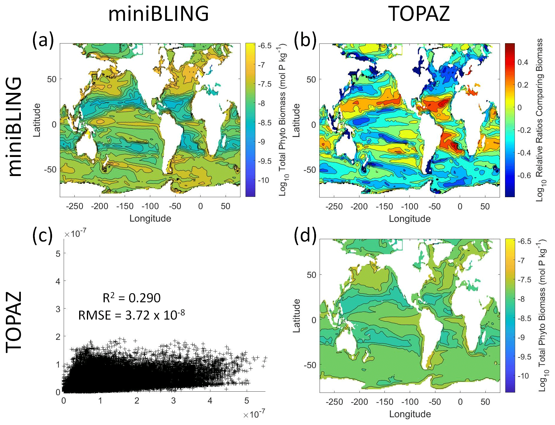
Figure 12 Comparison of the ESMs for total phytoplankton biomass in Case 3 in which circulation is given by ESM2Mo, but the BCs are different. The units for biomass in all panels are mol P kg⁻¹. The panels show point-by-point scatter plots comparing the ESMs against one another (c), yearly averaged log₁₀ biomass plots for each ESM (a, d), and the log₁₀ relative ratios comparing the yearly averaged contour plots of the ESMs (b). The x axis and y axis of the scatter plots (c) correspond to the horizonal and vertical ESM labels, respectively (e.g., panel c shows the miniBLING simulation on the x axis and the TOPAZ simulation on the y axis). The yearly averaged log₁₀ contour plots (a, d) correspond to the matching horizontal and vertical ESM labels (e.g., panel a shows the yearly averaged log₁₀ biomass of miniBLING). The log₁₀ relative ratios (b) were calculated as the ESM listed on the horizontal axis divided by the ESM listed on the vertical axis (e.g., panel b shows TOPAZ divided by miniBLING).

Table 5 The performance metrics for the NNEs being used to predict the outcome of the other ESM of Case 3. In the top half of the table, the R² and RMSE are listed. The values in parentheses are the values from comparing the respective ESMs against one another (these are the same values listed in the respective scatter plot in Fig. 12). The values outside the parentheses are the values from using the trained NNE of the ESM listed in the row to predict the outcome of the ESM in the column (e.g., the NNE trained on the TOPAZ simulation was used to predict the outcome of the miniBLING using the predictor values computed using the miniBLING simulation; these values were compared against the actual values of the miniBLING simulation to compute the RMSE of $\mathrm{3.91}\times {\mathrm{10}}^{-\mathrm{8}}$). In the bottom half of the table is the percent decrease in RMSE from the number listed inside the parentheses to the RMSE outside the parentheses (a negative percent means that the error increased).

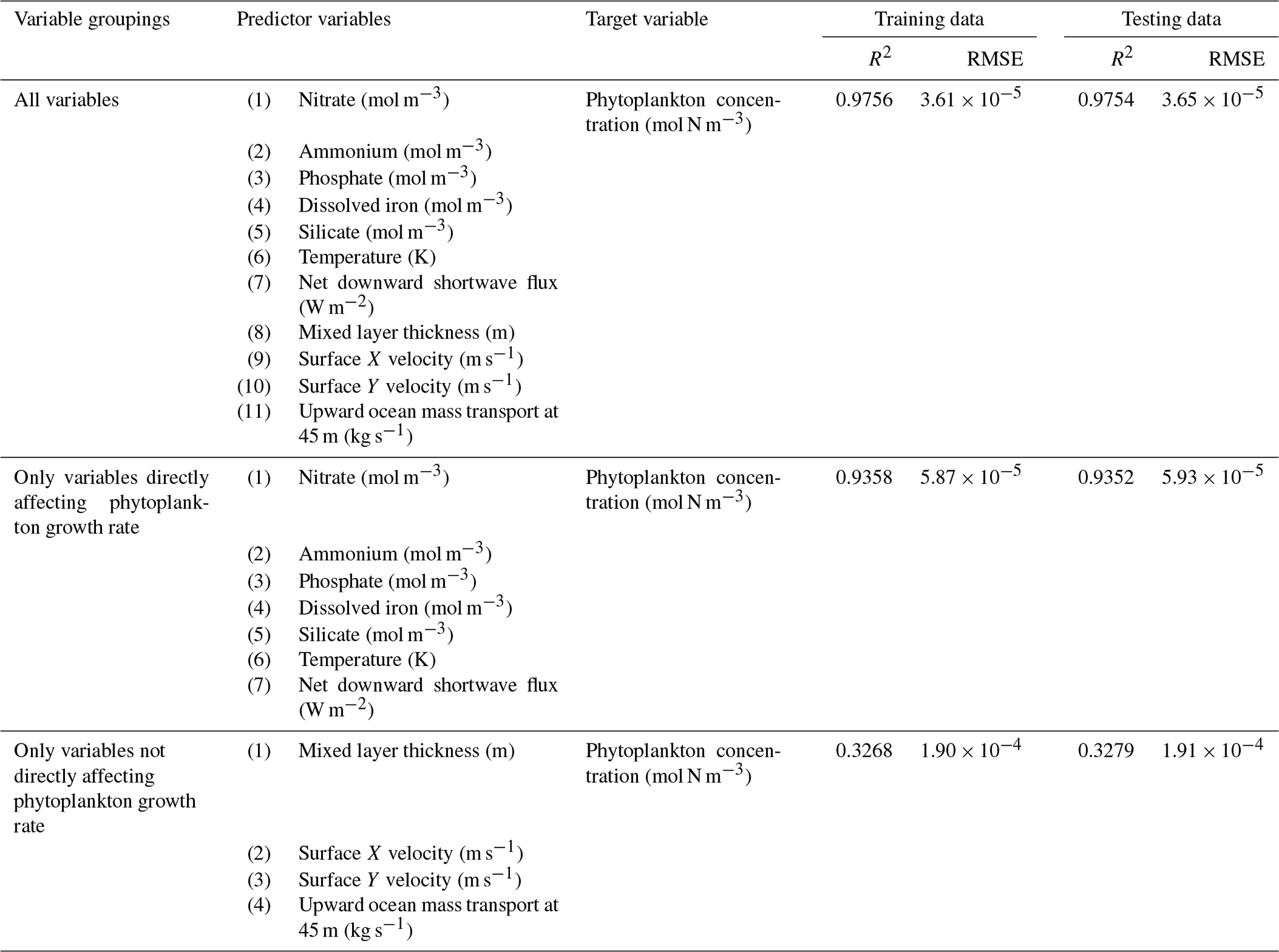
The challenge of comparing the results of different ESMs is evident in Case 3. For example, the performance metrics for the model runs in Cases 1 and 2 are relatively high in both the training and testing subsets, but the performance metrics for the TOPAZ simulation in Case 3 are much lower (R²>0.97 vs. ∼0.58, respectively; Table 2). From these results alone, it is unclear whether this drop in performance is because we are unable to characterize the TOPAZ simulation with NNEs using predictors common to both runs or whether we simply do not include enough relevant variables. To understand this, we perform a brief analysis in which we train NNEs on specific variables and measure their performance with ESM output from CMIP5 ESM2M, which has TOPAZ as its BC (Table 6). One NNE is trained using only variables that directly affected the phytoplankton growth rate (biology), one is trained using only variables that do not directly affect the growth rate (physics), and another is trained with both sets of variables (all). Our results indicate that we are able to characterize ESM2M (and, by extension, results produced by using TOPAZ as a BC) with NNEs with the inclusion of more relevant variables, such as nitrate, ammonium, and silicate (RMSE $\sim \mathrm{5.90}\times {\mathrm{10}}^{-\mathrm{5}}$ mol N m⁻³ – Table 6 – vs. the average biomass value of $\mathrm{3.14}\times {\mathrm{10}}^{-\mathrm{4}}$ mol N m⁻³). Without the inclusion of all the relevant variables as predictors, the performance of the NNE trained on output from the TOPAZ simulation suffers compared to the NNE trained on the miniBLING simulation.

Table 6 The performance metrics for the training and testing subsets of NNEs trained on different variable combinations of CMIP5 ESM2M output and details about the predictor and target variables.

An additional challenge with comparing different ESMs is that certain variables may not be present in all ESMs. For example, one ESM may have phosphate included as a variable and another ESM may not. This presents a problem when using the sensitivity analyses because each NNE needs to be presented with the same conditions for direct comparability. One potential method for mitigating this could be to use proxy variables such that variables not common to both ESMs could be modified to represent the missing variables. For example, if one ESM has phosphate as a variable and another ESM does not, it might be possible to modify a variable that would be equivalent to phosphate, such as nitrate. Using the Redfield ratio of 16:1 for the N:P ratio, the nitrate variable could be divided by 16 and thus be considered a proxy variable for phosphate. This proxy phosphate variable could then be used in training the NNE particular to the applicable ESM, so all NNEs would be trained using the same predictors.

5 Summary and conclusions

A challenge of using ESMs is understanding why different ESMs yield different results, even when they are run under similar conditions. Our objective with this paper was to investigate the extent to which NNEs could characterize differences across ESMs through differences in circulation vs. differences in biological formulations. We approached this objective by exploring three cases.

1. In the first case, we compared three configurations of an ESM that had identical intrinsic biological relationships but different physical circulations. The purpose of this case was to quantify the extent to which differences in physical circulations between model runs of the same ESM could affect the apparent relationships found by NNEs.

2. In the second case, we compared two model runs from the same ESM, except that the intrinsic biological equations were different, and the physical circulations were similar. The purpose of this case was to quantify the extent to which NNEs found differences in the apparent relationships and the size of those differences.

3. In the third case, we used two different ESMs that had different intrinsic biological relationships but identical physical circulations. The greatest difference between them was that in one ESM (ESM2Mo with TOPAZ as BC), biomass was able to be advected and diffused, making it a function of nutrients, irradiance, and circulation. This was in contrast to the other ESM (ESM2M with miniBLING embedded as BC) for which biomass was only a function of nutrients. The purpose of this case was to apply what we had learned in the first two cases to a more realistic ESM to quantify differences in the apparent relationships and identify any challenges.

Our results indicated that when all the relevant variables were included as predictors, the NNEs served as a parsimonious representation of the ESMs. With the first and second cases, NNEs were able to attribute differences between the model runs to physics and biological factors, respectively. The third case demonstrated that NNEs could be used to compare apparent relationships between different ESMs and find their key differences, along with highlighting some of the challenges in applying this to more realistic models.

The results of our study suggest that oceanographers and climate scientists could use the methods we have demonstrated to compare apparent relationships between ESMs, in addition to using spatiotemporal distributions and time series. This is not to say that spatiotemporal information is not important; rather, the relationships and spatiotemporal information can be used to inform one another. For example, in a side-by-side comparison of contour plots between biomass and nitrate concentrations, one might expect to see high biomass in high-nitrate regions. However, if low biomass is observed in a high-nitrate region, this would suggest that another factor (such as phosphate) is limiting phytoplankton growth. By visualizing the apparent relationships, one would be able to observe that phosphate has a strong limitation factor on the phytoplankton. This could then be verified with the spatial contour plot of phosphate against the original biomass and nitrate contour plots.

In addition to comparing relationships between ESMs, the methods presented here can allow for the comparison of relationships found in observational datasets to the relationships in ESMs, allowing for better tuning of the models and more accurate representations of the natural world as well as what changes we might expect under climate change. Our results here show the “best case” for comparing models with observations. The prevailing assumption is that environmental conditions set biomass and that ecological details do not matter; if two places have the same nutrients, irradiance, and mixing, they will have the same phytoplankton biomass. Our methods demonstrate that we can evaluate the extent to which such dynamics usually hold. In a follow-up paper, our preliminary results show that these methods can explain a large portion of the variance (60 %–80 %) in two satellite-derived observational datasets, along with greater than 90 % across a suite of CMIP6 ESMs.

Appendix A

This Appendix provides additional information about the datasets used in each of the three cases, along with information about how each dataset was randomly sampled.

The sizes of the datasets were as follows: 77 328 data points for each model run in Case 1, 77 328 data points for each model run in Case 2, and 577 332 data points for each model run in Case 3. Each dataset was split into training and testing subsets with 60 % of the full dataset going to the training subset and 40 % going to the testing subset. The training subset for each model run contained 46 397 data points in Case 1, 46 397 data points in Case 2, and 364 399 data points in Case 3. The testing subsets for each model run contained 30 932 data points in Case 1, 30 932 data points in Case 2, and 230 934 data points in Case 3.

The composition of the training and testing subsets was determined by random sampling such that the full dataset was randomly sampled in both space and time. Specifically, the random number generator function for MATLAB (2019b) was set to “twister” and the seed was set as “123” for reproducibility. Each data point was either part of the training subset or the testing subset; no observations were part of both.