Deep-learning spatial principles from deterministic chemical transport models for chemical reanalysis: an application in China for PM_2.5

Well-estimated air pollutant concentration fields are critically important to compensate for observations that are only sparsely available, especially over non-urban areas. Previous data fusion methods generally used statistical models to relate observations of target variables to proxy data and supporting variables at known stations. In this study, we developed a new data fusion paradigm by designing a deep-learning model framework and workflow to learn multivariable spatial correlations from chemical transport model (CTM) simulations, before using it to estimate PM_2.5 reanalysis fields from station observations. The model was composed of two modules as an explainable PointConv operation to pre-process isolated observations and a regression grid-to-grid network to build correlations among multiple variables. The model was trained with only CTM simulations and supporting geographical covariates. The trained model was evaluated in two aspects of (1) reproducing raw PM_2.5 CTM simulations and (2) generating reanalysis and fused PM_2.5 fields. First, the model was able to reproduce the CTM simulations well on a full domain from sampled CTM data items at sparse locations with an average R²=0.94 and RMSE = 4.85 µg m⁻³. Second, the fused PM_2.5 fields estimated from observations achieved a good performance with R²=0.77 (RMSE = 14.29 µg m⁻³) and R²=0.84 (RMSE = 12.96 µg m⁻³) respectively evaluated at the stringent city level and station level. The generated reanalysis PM_2.5 fields have complete spatial coverage within the modeling domain. One significant benefit of the fusion framework is that the model training does not rely on observations, which can be used to predict PM_2.5 fields in newly set up observation networks such as those using portable sensors. Meanwhile, in the prediction procedure, only station observations are used along with supporting covariates. The fusion model has high computing efficiency (< 1 s d⁻¹) due to acceleration using a graphical processing unit (GPU). As an alternative to generate chemical reanalysis fields, the method can be readily implemented in near-real time and be universally applied for other simulated variables with measurements available.

1 Introduction

Pollutant concentration fields with high accuracies are important for evaluating health effects, climate changes, and agricultural studies (Bell et al., 2007; Donkelaar et al., 2015; Gao et al., 2017). A long-term and reliable air quality dataset could also be used to assess pollutant emission control measures (Wang et al., 2010). The data fusion method has been widely used to obtain accurate and spatially complete datasets, such as fusing air quality model simulations and station air pollutant observations to estimate fine-scale air pollutant concentration fields (Berrocal et al., 2012; Rundel et al., 2015).

Most previous studies similarly used a general paradigm to develop well-estimated air pollutant concentration fields. In this paradigm, statistical models were trained to describe nonlinear relationships between observations and proxy data as well as supporting variables at the locations of observation sites (Berrocal et al., 2012; Lyu et al., 2019; Chu et al., 2016). The widely used proxy data for PM_2.5 concentrations include aerosol optical depth (Lv et al., 2016) and chemical transport model (CTM) simulations (Lyu et al., 2019). Popular statistical models include the linear mixed-effect model (Hao et al., 2016), machine learning models of random forest (Brokamp et al., 2018; Huang et al., 2021), deep neural networks (Qi et al., 2018), and ensemble models (Xiao et al., 2018). The fitted models were then used to predict the concentration field of target variables in the whole area directly or through spatial spreading techniques such as Bayesian estimation (Xu et al., 2016), partial linear regression (Wang et al., 2016), and distance-constrained interpolations (Chang et al., 2014; Friberg et al., 2016).

Even though many datasets have been developed through deliberately designed statistical models, long-term observations, and extensive explanatory variables, there are scientific gaps in many circumstances following this paradigm to develop air pollutant fields. First, these models usually rely on long-term and large-scale station observations for training, especially for complex time- and space-resolved models (Feng et al., 2020; Huang et al., 2021). For newly set up, temporal, or mobile observation networks, there would be limited datasets for training effective data fusion models. Second, most of the previous methods cannot fuse observations of multiple variables well from different monitoring networks. For example, stations in air quality and meteorology observation networks are usually not spatially aligned. The observations in two networks could not be directly fused in current models well. Instead, meteorology reanalysis data were often used as important explanatory variables in previous fusion models (Geng et al., 2015; Ma et al., 2015; Wei et al., 2021). However, in near-real-time operational data fusion applications, these reanalysis data would be unavailable or require intensive computations. Last but not least, most of the previous methods that fuse CTM simulations rely on relatively accurate and stable simulation data to achieve good fusion performance (Tong and Mauzerall, 2006). Consistency in CTM parameters, configurations and inputs are also strictly required to guarantee stable fusing performance. Especially in near-real-time operational data fusion applications, adjoint models need to be running simultaneously (Friberg et al., 2016), which is costly in computations.

To address these scientific gaps, this study proposes a new data fusion paradigm by designing a deep-learning-based model framework to estimate reanalysis from station observations by learning spatiotemporal correlations from deterministic CTM models. Distinct from the existing data fusion models, the data fusion model does not use any station observations to fit. Instead, the deep-learning network was trained with only CTM model simulations to learn their dynamic spatial correlations, which is backed by the CTM's first principles. In the prediction procedure, the fusion and reanalysis data are then generated by the trained model by applying the learned dynamic correlations to real observations. The model framework is fundamentally an alternative of generating chemical reanalysis fields but without rerunning CTMs with data assimilation.

2 Data and methods

2.1 CTM simulations

In this study, the data fusion model was trained to learn spatial correlations of multiple variables from CTM simulations. The simulated PM_2.5 and other meteorological variables in 2016–2020 were produced using a modeling system that consists of three major components: the meteorology component (WRFv3.4.1) provides meteorological fields, the emission component provides gridded estimates of hourly emissions rates of primary pollutants that match model species, and the CTM component (CMAQ v5.0.2; Byun and Schere, 2006) solves the governing physical and chemical equations to obtain 3-D pollutant concentrations fields at a horizontal resolution of 12 km. The system was operated in forecasting mode, which produces CTM simulations for 5 d ahead each day. Therefore, corresponding to each day, there are five CTM simulations with different forecasting lead time. The CTM simulations of PM_2.5 concentrations have reasonable performance when evaluated against surface measurements, with root mean square error (RMSE) being 29.28–31.08 µg m⁻³ and coefficient of determination (R²) being 0.31–0.42 (Fig. S1 in the Supplement). The data covered all of China with 372×426 12 km by 12 km grid cells. Simulation data in the 2016–2019 period were used as the training dataset, while the 2020 simulation data were used for evaluation.

We used the simulated daily mean surface-layer PM_2.5 concentrations, relative humidity (RH), and wind speed (WS) in the data fusion model. The two meteorological variables are selected because they exhibited stronger correlations with PM_2.5 concentrations (Fig. S2). Precipitation is found not to be well correlated with PM_2.5 concentrations. Boundary layer height (PBL) has relatively strong correlations with PM_2.5 concentrations, but PBL observation data are not commonly available like other meteorological variables such as RH and WS. Therefore, precipitation and PBL were not included in the model. The air temperature was not included in the model either because it is highly correlated with surface elevations.

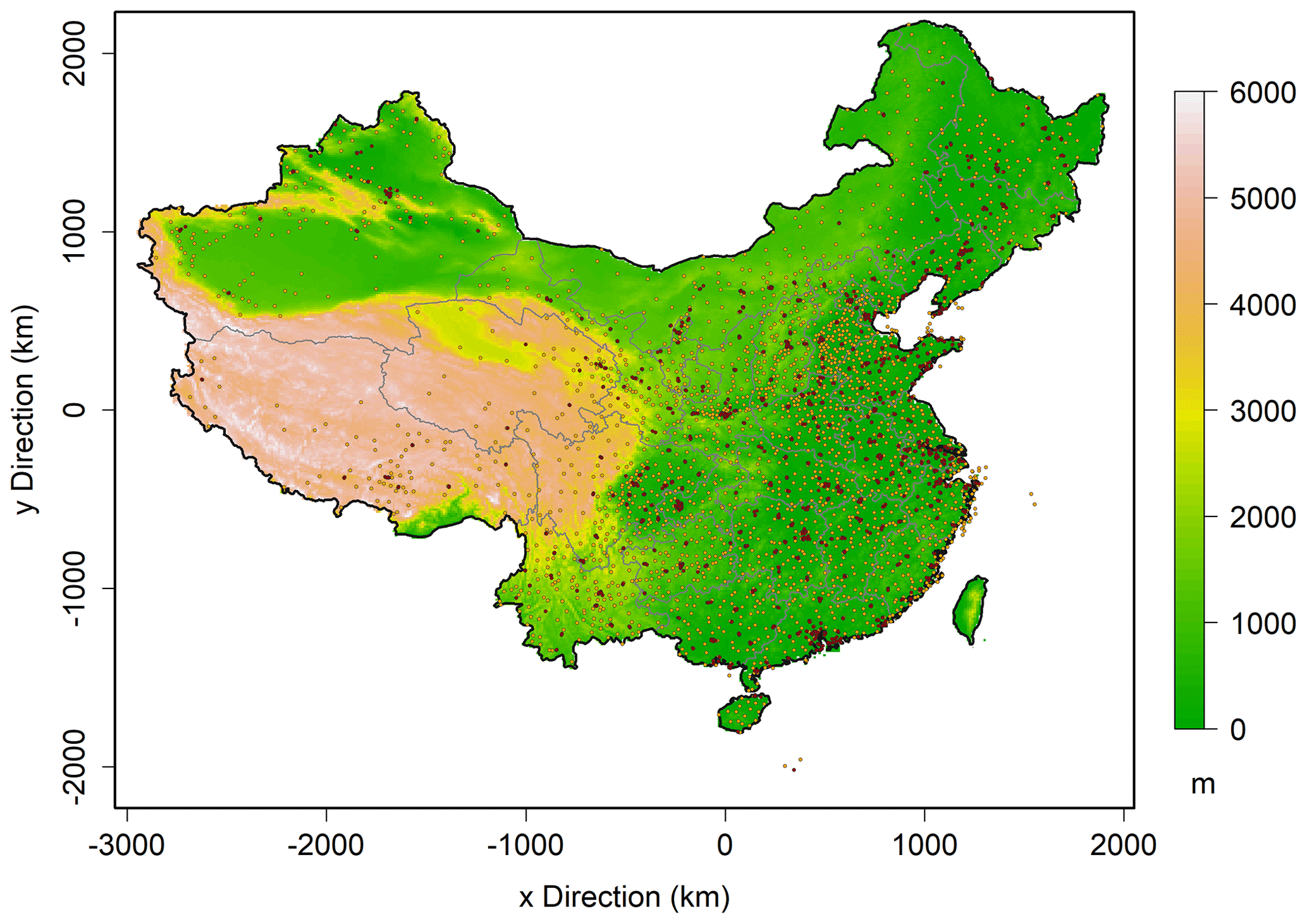
Figure 1 A map of the study area with elevation in color. Dark red dots represent the national PM_2.5 monitors, and orange dots refer to national meteorological stations.

2.2 Ground observations

PM_2.5 observations in 2020 were obtained from the China National Environmental Monitoring Center (CNEMC) (http://106.37.208.233:20035/, last access: 21 February 2021) with the monitoring network as exhibited in Fig. 1. Meteorological variables of daily mean RH and WS for the same period from national meteorological observing stations were obtained from the China Meteorology Agency (CMA) network (Fig. 1). Geographical variables such as the surface height of the digital elevation model (DEM) as well as land use and land cover (LULC) (Zhang et al., 2021) were also used in this study for fusion. From LULC, the fraction of urban area is used to indicate emission strengths. These data variables were resampled to the aforementioned CTM simulation grid.

The raw data for PM_2.5 and meteorology data were hourly, which were averaged to a daily mean if there were more than 18 valid hourly observations in a day at the local time at each monitor. Each of these data items at each station was assigned to a grid that was defined the same as used in the CTM simulations. For the sites that co-located in the same grid cell, their averages were used. It should be noted that grid cells with no valid observations within them were filled with zeros. In this way, each variable of PM_2.5, RH, and WS will have one gridded observation field in each day.

2.3 Deep-learning data fusion framework

The task of obtaining a spatially complete air pollutant field from point observations can be regarded as solving a downscaling problem, which means that data values in gap areas among stations need to be optimally estimated from known sparse measurements based on physical or statistical constraints. Most previous studies use statistical methods to relate observations to other supporting variables at stations (Di et al., 2016; Beloconi et al., 2016). In this study, we built a point-to-grid downscaling model by learning from CTM simulations to generate gridded data fusion fields from station observations.

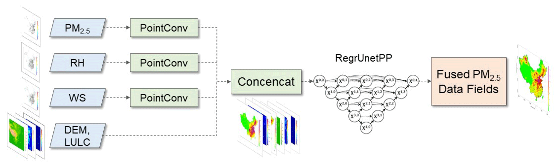
Figure 2 Data fusion framework using station observations of multiple variables to obtain gridded fields of PM_2.5.

A new deep-learning model workflow (Fig. 2) was designed to fulfill the task of point-to-grid data fusion and downscaling. This deep-learning model includes novel point convolutional (PointConv) operations and a backbone fusion module of regression using Unet++ (RegrUnetPP). The PointConv is designed for handling spatially isolated and irregular station observation data to compensate for the efficacy loss of ordinary convolutions in processing these data. In traditional convolutional operations, 3×3 filters are often used to calculate a moving sum, which would lose effectiveness when it comes to spatially imbalanced station observations. For example, when convolutional filters move to areas without observations, the result will be zero. However, if the convolutional filters work in areas with dense observations, the results will become significantly larger. Therefore, they will generate spatially biased and distorted results (Qi et al., 2018). To solve the problem, we proposed a novel and interpretable PointConv operation to handle isolated station observations of multiple variables. The successive PointConv operation is defined as follows.

$$\begin{array}{}\text{(1)}& {\displaystyle }{\text{PointConv}}_{\mathrm{1}}\left(x\right)={\displaystyle \frac{\text{Conv}\left(w_{n\mathrm{1}},x\right)}{\text{Conv}\left(w_{n\mathrm{1}},x\mathit{\_}\text{one}\right)+e^{-\mathrm{5}}}}\text{(2)}& {\displaystyle }{\text{PointConv}}_{\mathrm{2}}\left(x\right)={\displaystyle \frac{\text{Conv}\left(w_{n\mathrm{2}},{\text{PointConv}}_{\mathrm{1}}\left(x\right)-x\right)}{\text{Conv}\left(w_{n\mathrm{2}},x\mathit{\_}\text{one}\right)+e^{-\mathrm{5}}}}\text{(3)}& {\displaystyle }\text{PC}\left(x\right)={\text{PointConv}}_{\mathrm{1}}\left(x\right)+{\text{PointConv}}_{\mathrm{2}}\left(x\right)\end{array}$$

Here, w_n refers to a convolutional filter with a size n. The Conv(w_n,x) in Eq. (1) refers to the ordinary convolution on x with filters w_n, which are station observations assigned to predefined grid cells. The x_one was binarized from x by replacing grid cells with valid observation data in x as 1. The PointConv was conducted by mimicking successive analysis procedures as in Eq. (2). The PointConv filter size in the two steps was determined to be 21 and 11, respectively, for n₁ and n₂. In summary, this PointConv operation has the following features and advantages compared to conventional convolutions.

1. The weighted average of isolated data items is calculated rather than a weighted sum by only considering valid data.

2. Large-sized filters are used to learn and represent spatial correlations well within a large area.

3. Successive PointConv operations are implemented to better reflect spatial variations in local scales.

4. Multivariable observations could be handled separately and simultaneously even if they are from different networks.

The PointConv filters in well-trained models are expected to have larger values in the center area and lower values in the outer area. With the PointConv module, a spatially complete gridded dataset is constructed for three observational variables, denoted as PC(PM_2.5), PC(RH), and PC(WS). By binding PointConv results of different variables of PM_2.5, RH, and WS with other static supplementary data such as DEM and LULC, input data to the data fusion module RegrUnetPP are built. The whole data fusion model could be summarized as in Eq. (4).

$$\begin{array}{}\text{(4)}& {\displaystyle }\begin{array}{rl}{\widehat{y}}_{{\mathrm{PM}}_{\mathrm{2.5}}}& =\text{RegrUnetPP}\left(\text{Concencat}\left(\text{PC}\left({\text{PM}}_{\mathrm{2.5}}\right),\text{PC}\left(\text{RH}\right),\right.\right.\\ & \left.\left.\text{PC}\left(\text{WS}\right),\text{DEM},\text{LULC}\right)\right)\end{array}\text{(5)}& {\displaystyle }\text{loss}={\displaystyle \frac{\mathrm{1}}{N}}\sum _{i=\mathrm{1}}^N\left|y_{{\text{PM}}_{\mathrm{2.5}},i}-{\widehat{y}}_{{\mathrm{PM}}_{\mathrm{2.5}},i}\right|\end{array}$$

The operation Concencat refers to binding data fields of different data variables into one multiple-channel dataset. The ${\widehat{y}}_{{\mathrm{PM}}_{\mathrm{2.5}}}$ refers to the estimated PM_2.5 concentrations, and $y_{{\mathrm{PM}}_{\mathrm{2.5}},i}$ refers to the original CTM simulations with N equal to the number of total grid cells.

The fusion module can be any grid-to-grid deep-learning model to estimate fused PM_2.5 concentrations ${\widehat{y}}_{{\mathrm{PM}}_{\mathrm{2.5}}}$. Here we used a regression Unet++ model (Zhou et al., 2018), i.e., RegrUnetPP. The RegrUnetPP model was designed as an encoding–decoding type of network developed from Unet (Ronneberger et al., 2015). Many skip-connection modules (Jin et al., 2017) were added in the RegrUnetPP (Fig. 2) to fully explore spatial correlations on different scales while keeping abundant details in output results. RegrUnetPP was constructed by replacing the SoftMax activation layers with the ReLU layers and adopting a mean absolute error (MAE) loss function (Eq. 5) instead of the original MaxEntropy function.

2.4 Model training

The model was trained with the 1 d lead CTM simulations of PM_2.5, RH, and WS, together with geophysical covariates of DEM and LULC. Since 4-year data for 2016–2019 have been used to train the model, the whole training dataset has a data shape of $R^{\mathrm{1461}\times \mathrm{372}\times \mathrm{426}\times \mathrm{5}}$. Considering that the deep-learning model needs to learn point-to-grid spatial correlations from CTM simulations, nominal “station” data were constructed by randomly sampling 1500–2500 data points from gridded simulation data separately for each variable at each time, while raw spatially complete PM_2.5 simulation data were used as the target gridded “truth” data. The sampling data point number of 1500–2500 was determined according to the actual air quality monitoring station density in middle and eastern China. There are around 700 grid cells with air quality monitoring stations in middle and eastern China within an area of around 4 million km². Considering the total area of 9.6 million km² in China, the sampling size was set to be random integers in a range of 1500–2500 to ensure that sampling point densities are at a similar level as the density of actual monitoring stations. The sampling size was randomly determined for each training batch (i.e., each day); as such, the total number of training data points did not vary much among different years.

The spatial correlations of CTM simulations are backed by physical and chemical principles comprehensively represented in the WRF-CMAQ model. The fusion model was trained with the WRF-CMAQ CTM simulations within China from 2016 to 2019 for 20000 iterations with a batch size of 10 when the loss function became stable in about 2 h running on a NVIDIA RTX GeForce 2080Ti GPU card. It should be noted that the observation data were not involved in the model training procedure at all. In the model prediction procedure, actual station observations will be used as input to generate fused PM_2.5 concentration fields. We also trained the model with the 5 d lead CTM simulations for the purpose of evaluating impacts from meteorological uncertainties. Note that each of the 1–5 d lead time CTM simulations is driven by different meteorological forecasts, with 1–5 d lead time, respectively. The meteorological uncertainties associated with the 5 d lead CTM simulations are usually higher than those with the 1 d lead CTM simulations.

2.5 Model evaluation

In general, the evaluation was conducted for 2020, which is independent from the training data period of 2016–2019. Specifically, the fitted fusion model was evaluated in two aspects. Firstly, its capabilities to predict the fully gridded model simulations from isolated sampled simulation data items were assessed using the CTM simulation data in 2020. In this aspect, the station-wise CTM PM_2.5 simulations were constructed by sampling data in grid cells with CNEMC stations (for PM_2.5) or CMA stations (for RH and WS) from raw gridded simulations. By feeding these station-wise simulations and supporting variables into the fusion model, spatially completed gridded data are obtained. The fused simulation data are then compared against the corresponding raw CTM PM_2.5 simulations. The comparison was performed each day, since there are sufficient data items in daily simulations. It should be noted that only grid cells located in mainland China were compared. Statistical metrics of the coefficient of determinant (R²), root mean square error (RMSE), and normalized mean absolute error (NME) were calculated for performance evaluation.

For the second aspect, data fusion model performance was evaluated with real station observations using two cross-validation methods. Specifically, leave-stations-out cross-validation methods (LSCV) and stringent 10-fold leave-cities-out cross-validation (LCCV) were used to evaluate model performance (Lv et al., 2016). In the LCCV method, all cities with PM_2.5 stations were randomly split into 10 groups, while in the LSCV method all stations were randomly split into 10 groups. PM_2.5 observations in one group of stations were used as independent evaluation data, while the data in remaining nine groups were used in data fusion. This process was iteratively performed 10 times to ensure all groups of data have been used for evaluation. Considering that the air quality stations are mostly clustered in urban areas, the LCCV method will better reflect the model's performance in predicting PM_2.5 concentrations in remote rural areas than the station-based LSCV method. Statistical metrics of R², RMSE, and NME are also used for statistical measures.

Figure 3 PointConv filters for PM_2.5, RH, and WS.

3 Results and discussion

3.1 Model parameters

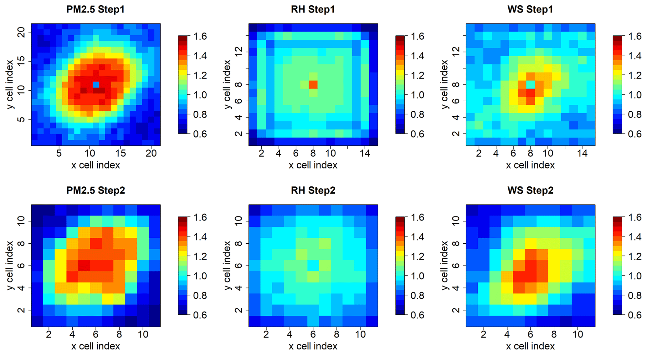
According to its definition, the PointConv was interpretable due to its dedication to implementing an interpolation-like process from station observations to remove imbalanced, sparse and clustering distributions of station data items. In fact, the large filters in PointConv resemble covariance functions on distances in common spatial interpolation methods. Larger values in the central area of PointConv filters (Fig. 3) indicate that spatial correlations are stronger in closely neighboring data items (Shepard, 1968) than those at long distances. The central values of PointConv filters are respectively around 1.5, 1.1, and 1.4 for PM_2.5, RH, and WS in both steps. The filters' distribution also revealed that the influencing distance for PM_2.5 is around 6 grid cells, which was equivalent to 72 km in terms of the 12 km resolution. For RH, the spatial correlations are weak considering that filters were more spatially uniform as exhibited in Fig. 3. For WS, it exhibited a stronger locality as indicated by the smaller hot-spot areas with a radius around 4 grid cells (∼48 km).

The filters were generally isotropic with slightly larger values in the northeast–southwest direction than in other directions, which could be caused by topographic and climatic patterns in our study area. The slightly anisotropic pattern still existed when wind direction was considered (Fig. S3). Compared to traditional distance-related interpolation methods such as kriging and inverse distance weighting (IDW) (Friberg et al., 2016), the anisotropy of the filters indicated the PointConv's capability to characterize relatively complex spatial correlations.

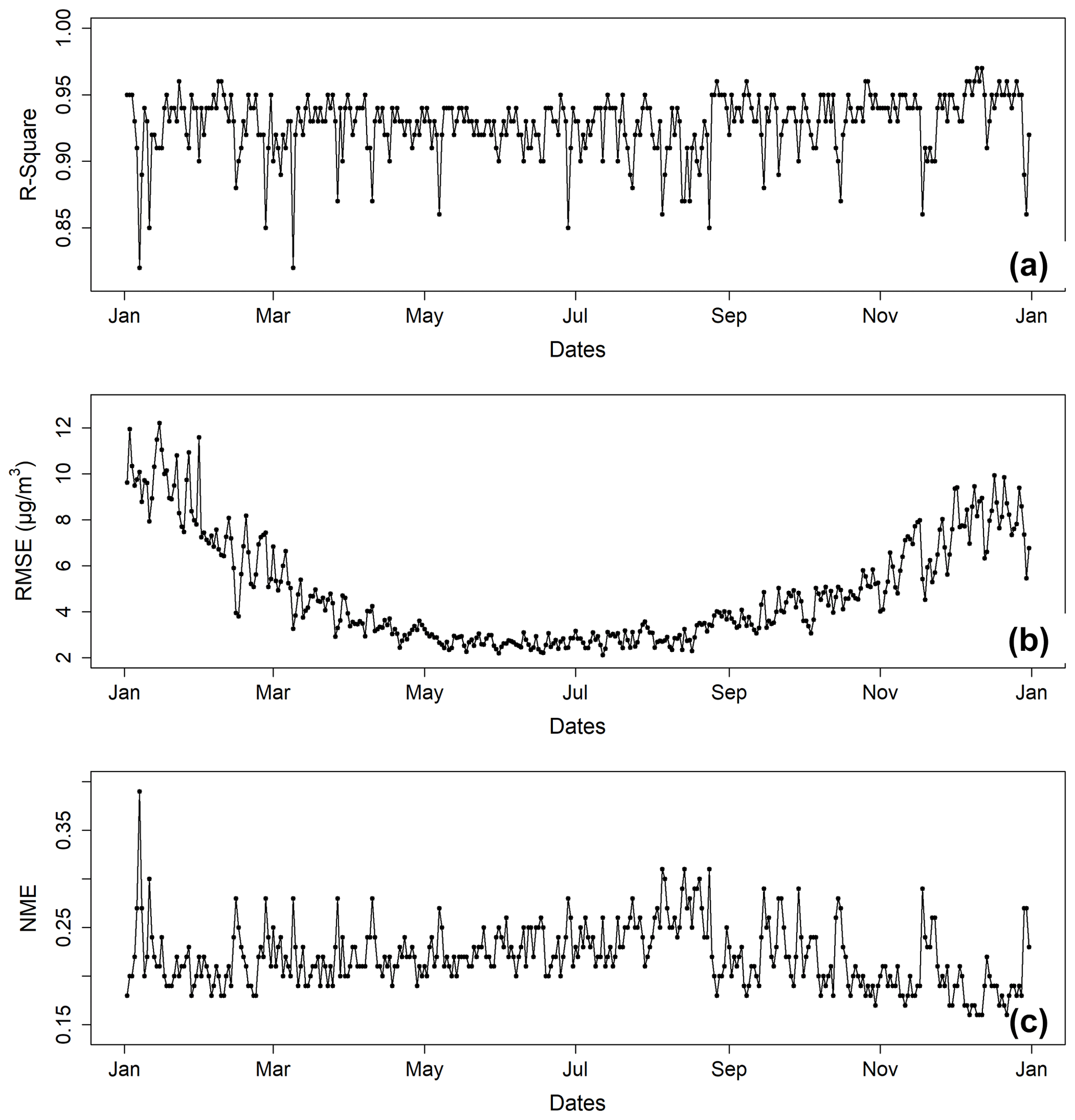
Figure 4 Daily prediction performance evaluated against the raw PM_2.5 CTM simulations in 2020: (a) R², (b) RMSE, and (c) NME.

3.2 Model performance for reproducing simulation fields

Our data fusion model has very high accuracies in predicting and/or reproducing fully gridded PM_2.5 CTM simulations as exhibited in Fig. 4, even though only ∼800 PM_2.5 data points in grid cells with observation stations were used to estimate data values in the China nationwide 64 488 grid cells. The averages of daily R², RMSE, and NME values were respectively 0.94, 4.85 µg m⁻³, and 0.22 in 2020. The good evaluation metrics indicate the strong capability of the trained deep-learning data fusion model to reproduce the spatial correlations among multiple variables of the CTM simulations. The fusion model has a stable performance in terms of R² and NME values. There are occasional days on which R² values are at low levels of ∼0.85. On these days, PM_2.5 pollution patterns change fast, which were generally less trained compared to days with more stable patterns.

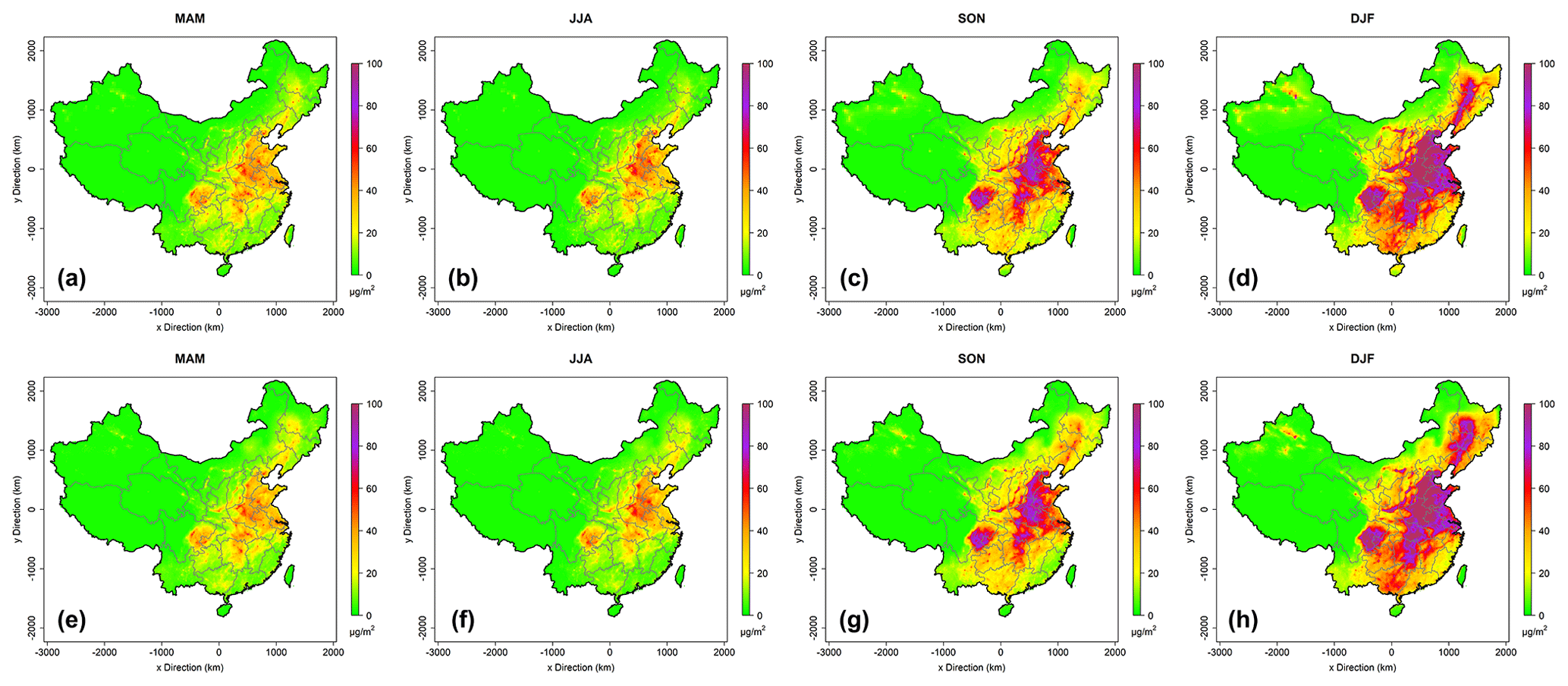
Figure 5 The seasonal average PM_2.5 concentrations of the raw CTM simulations (a–d, first row) and the reproduced simulations using the data fusion model (e–h, second row).

By comparing the raw daily average PM_2.5 CTM simulations and the reproduced PM_2.5 fields from ∼800 data points (Fig. 5), it can be concluded that they exhibited high correlations and similarities. The fusion model fully reproduced the raw CTM simulations in terms of concentration levels, spatial patterns, and fine-scale hot spots, indicting the data fusion model's capabilities to encode high-level and detailed spatial correlations. By giving the fusion model only a small portion of simulations at sparsely scattered locations, it can reproduce the entire whole-domain simulation dataset accurately.

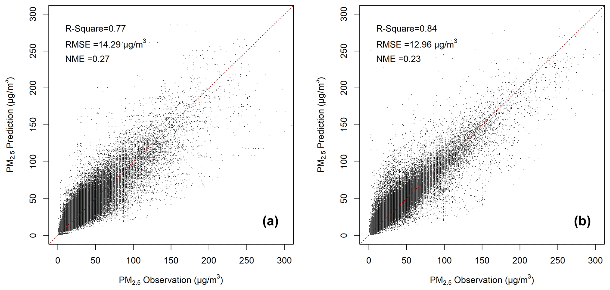
Figure 6 Scatter plots of predictions versus observations respectively evaluated using the (a) LCCV and (b) LSCV methods.

3.3 Model performance for generating reanalysis fields

We implemented the data fusion model with the PM_2.5 and meteorological station observations in 2020 to generate the PM_2.5 reanalysis fields for evaluation. The evaluation results exhibited good performance with R²=0.77 for the LCCV method and R²=0.84 for the LSCV method (Fig. 6), with the RMSE values being 14.29 and 12.96 µg m⁻³, respectively. Considering that most grid cells were located within city urban areas, actual model performance in the nationwide domain should be generally between the metrics by LCCV and LSCV, which is 0.77–0.84 for R², 12.96–14.29 µg m⁻³ for RMSE, and 0.23–0.27 for NME. Previous studies tend to underestimate PM_2.5 concentrations in severe pollution scenarios (Di et al., 2016; Senthilkumar et al., 2019). Our data fusion method predicted high-level PM_2.5 concentrations very well, with NME for the PM_2.5 concentration higher than 150 µg m⁻³ being small at 0.19 and 0.14, respectively, for LCCV and LSCV. It worth noting that there are increased errors from reproducing CTM simulations (R²=0.94) to generating reanalysis fields (R²=0.77–0.84). The difference of 0.1–0.17 should be mainly attributed to CTM simulation uncertainties of PM_2.5 spatial correlations compared to actual correlations in observations.

Our model has good performance compared to previous studies that used the spatial cross-validation method. For example, Lyu et al. (2019) used an ensemble deep-learning model to build relations between CTM simulations and observations of PM_2.5 in China with a performance of R²=0.64 and RMSE = 24.8 µg m⁻³ using a station-level evaluation method. Xue et al. (2019) fused aerosol optical depth (AOD), CTM simulations, and ground observations with a complex multi-stage model and achieved a good performance of R²=0.81 with the LSCV method. Xiao et al. (2018) built up an ensemble machine learning model to predict PM_2.5 at 0.1^∘ resolution with an accuracy of R²=0.76. Huang et al. (2021) used a multi-stage random-forecast-based model to predict a very high-resolution dataset and achieved R²=0.86 with the LSCV method.

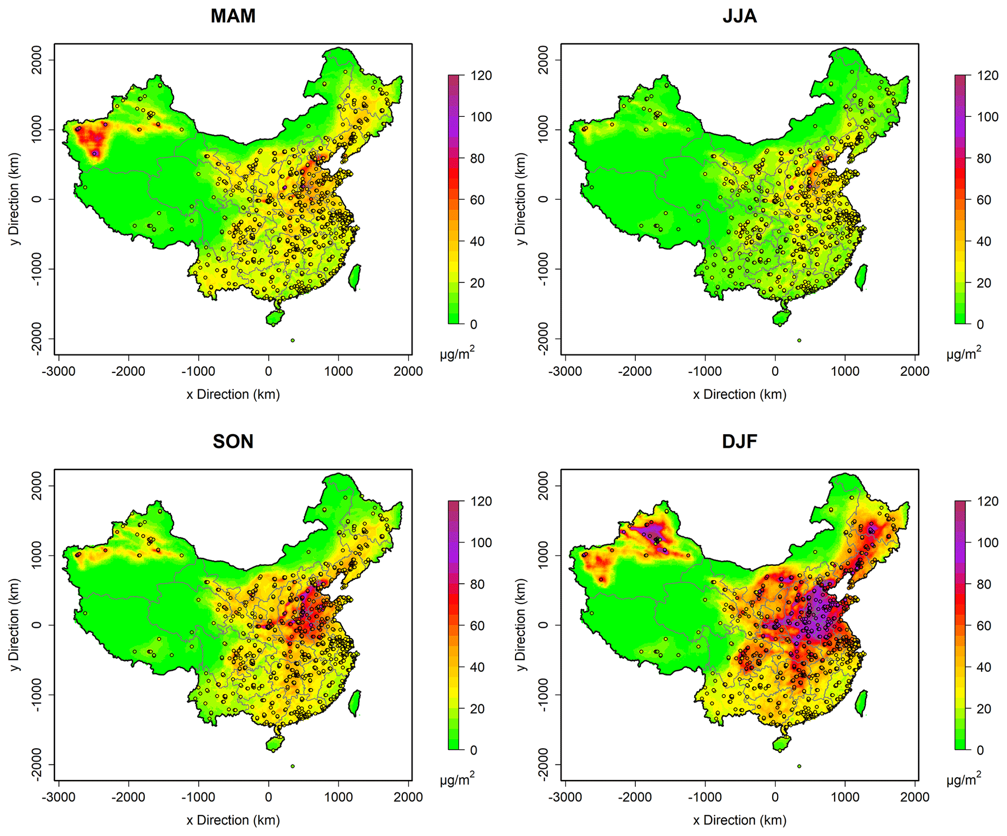
Figure 7 Reanalysis PM_2.5 concentration fields in four seasons in 2020. Circles with filled colors represent monitoring sites and corresponding observations.

Daily PM_2.5 reanalysis fields for 2020 were obtained with the model framework and station observations. Considering that the fused and reanalysis fields are complete in space, the high pollution levels in winter are clearly revealed in detail in the North China Plain (NCP) and in the long, narrow basin areas of Shanxi and Shaanxi provinces (Fig. 7). Also, unlike most previous studies (Huang et al., 2021), PM_2.5 concentrations in the high-altitude clean Tibetan Plateau region are predicted as low values, the same as observed. High pollution levels in the middle-western Inner Mongolia area of Hohhot, Baotou, and Yinchuan were also well captured in all four seasons.

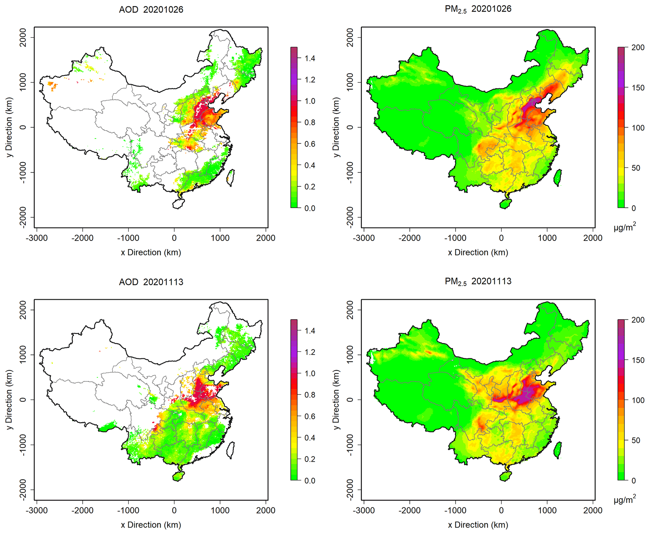
Figure 8 Comparison between MODIS AOD and PM_2.5 fusion data on 26 October and 13 November 2020.

To further evaluate the spatial distributions of the fused PM_2.5 fields, we compared them with the MODIS AOD distributions on the days with large AOD spatial coverage (Figs. 8 and S4). Spatial distributions of the fused PM_2.5 and AOD show high similarities with each other. For example, on 26 October, high PM_2.5 concentrations coincide with high AOD values in the NCP, especially in the areas along the eastern edge of the Taihang Mountains. In detail, PM_2.5 concentrations and AOD values are both relatively low in the Yimeng Mountains located in the middle-south of Shandong province. The high PM_2.5 concentrations in the basin area of Shanxi province are also higher than the surrounding area, consistent with those of AOD. For 13 November, PM_2.5 concentrations are extremely high in the NCP and high in the central China areas of Hubei and Hunan provinces, like the AOD values. Also, in the northeastern regions of Yunnan province, both PM_2.5 and AOD values are relatively high. The spatial coincidence of PM_2.5 concentrations and AOD values at all levels further validates the accuracy of the fused data.

4 Discussion

In this study, PM_2.5 fields are fused using multiple observational variables from different networks by developing a novel deep-learning data fusion model framework. The core of our fusion model is to learn and encode spatial correlations from CTM simulations to build connections between isolated data points with gridded data fields and among multiple variables. In other words, our method is to “interpolate” the isolated observations to achieve full spatial coverage by using the spatial correlations learned from the CTM simulations. The training is done only with the simulated data. Observational data are not used in the training procedure but only used in the prediction step. Then the trained fusion model is applied to predict reanalysis and fused data fields from isolated station observations by decoding the learned spatial correlations. As we have demonstrated, the method can accurately reproduce the whole-domain PM_2.5 concentration fields from only a small number of data points.

In previous studies, all variables needed to be spatially paired at stations first to train regression models (Lyu et al., 2019; Xue et al., 2019). To use data from different networks, interpolation and analysis or reanalysis needed to be carried out first, the procedure of which is disconnected from the data fusion model. Here, with the successive PointConv modules, it can fuse station data variables from different observation networks, even if they are not spatially aligned at co-locations. The PointConv modules were trainable as part of the whole deep-learning data fusion model. Without a data pairing procedure, the model training and prediction procedure became straightforward and only required the same spatial grid setting for all input variables.

As we stressed, this model was fitted with model simulation data by learning daily spatial patterns from long-term CTM simulations. It has two benefits. First, the trained deep-learning data fusion model can represent and reflect spatial correlations between PM_2.5 (and any other model species and/or variables as well) and its supporting variables by retaining physical and chemical principles in the WRF-CMAQ model. Hence, the method can be readily applied for other CTM-simulated species with measurements available. Second, it does not need any observation datasets to train the model. This is quite beneficial for data fusion applications, especially when station networks are newly set up or observations are from mobile or portable sensors. The data fusion models used in previous studies often require long-term observations (Wei et al., 2021; Huang et al., 2021; Xue et al., 2019), which makes it difficult to be reproducibly used in new applications. Conversely, our method is straightforward to use and can be easily examined by intercomparison with other methods. It provides a pre-trained deep-learning model for its application in other studies. To run this model, users only need air quality observations, meteorological observations, and static variables.

It worth noting that high fusion accuracy has been achieved even though the CTM simulations themselves have relatively low accuracies (Fig. S1). CTM simulation errors usually come from three major sources, which include meteorology uncertainties, emission inventory uncertainties, and imperfect atmospheric physical and chemical parameterizations. However, as we have stated above, the training here is purely to learn the spatial correlations among simulated variables from CTM simulations; the biases and errors in CTM simulation do not impact the training results. The nearly perfect reproduction of the 2020 simulations has demonstrated this.

To evaluate and/or separate fusion errors caused by meteorological uncertainties, we trained two data fusion models respectively using the 1 d lead CTM forecasting simulations and the 5 d lead CTM forecasting simulations. The 1 d lead forecasts have different but usually smaller errors than the 5 d lead forecasts (Fig. S1). As shown in Fig. S5 (see the Supplement), both trained models have similar performance in producing reanalysis fields. Considering that errors of simulations at different lead times are mainly caused by meteorological inputs, it revealed that CTM errors from meteorology do not have much influence on reanalysis performance.

As for the errors raised by emission uncertainties, we compared the performance of the reanalysis fields in February, March, and April 2020 against that in other months of 2020. In the 3 select months, air pollutant emissions in China dramatically decreased to a very low level due to a large-scale national lockdown to prevent the spreading of Covid-19. Compared to the other months without national lockdowns, emissions inventories used in CTM simulations should have significantly increased uncertainties during these 3 months. However, the reanalysis performance in the lockdown period does not decrease compared to that in other months as shown in Fig. S6 (see the Supplement). In fact, input changes in pollutant emissions and meteorological fields within the CTM simulations are allowed and should be encouraged to cover a wider range of emissions and meteorological scenarios to help improve the robustness of the trained model.

However, the uncertainties of physical and chemical parameterizations in the CTM could influence the reanalysis performance, as they determine the inherent spatiotemporal correlations among multiple variables. But their impacts on reanalysis performance here are expected to be small as well, provided the configurations in CTM simulations are not changed dramatically, because the nonuniformity of the biases and errors these parametrization uncertainties alone can cause in CTM simulations are expected to be even lower in magnitude. We do not recommend using totally different configurations in CTM simulations. Comparatively, in other observation–simulation regression methods, both model configurations as well as meteorology and emission inputs are required to be unchanged and relatively accurate in training datasets (Xue et al., 2017; Hao et al., 2016).

It also worth noting that the model framework in this study has the significant benefit of very high computational efficiency, with computing time for one-time fusion far less than 1 s running on the consumer GPU card of a NVIDIA 2080Ti.