CliffDelineaTool v1.2.0: an algorithm for identifying coastal cliff base and top positions

Correct quantification of coastal cliff erosion requires accurate delineation of the cliff face bounded by the cliff top and base lines. Manual mapping is time consuming and relies on the mapper's decisions and skills. Existing algorithms are generally site specific and may be less suitable for areas with diverse cross-shore cliff geometries. Here we describe CliffDelineaTool (v1.2.0), a MATLAB/Python-based algorithm that identifies cliff base and top positions on complex cliffs using cross-shore transects extracted from digital elevation models. Testing on four 750–1200 m cliffed coastlines shows that the model performance is comparable to manual mapping and provides some advantages over existing methods but provides poor results for cliff sections with ambiguous cliff top edges. The results can form the basis for a range of analyses, including coastal inventories, erosion measurements, spatiotemporal erosion trends, and coastline evolution modeling.

1 Introduction

Correct quantification of cliff erosion for scientific and management purposes requires accurate delineation of coastal cliff faces. Cliff base and top positions are often digitized manually on georeferenced maps, aerial photographs, orthophotographs, and digital elevation models (DEMs) (e.g., Dornbusch et al., 2008; Hapke et al., 2009; Brooks et al., 2012; Orviku et al., 2013; Swirad et al., 2017; Young, 2018). However, manual mapping is subject to the mapper's decisions and skills (Moore, 2000). The lack of uniform definitions for a cliff base and top leads to further inconsistencies. Payo et al. (2018) suggested that, for consistency, the mapping should be performed at the same time for the entire dataset, and by one mapper. However, this becomes problematic for multitemporal studies, and those that build on previous efforts.

While manual digitization may be necessary when using cartographic sources, DEMs provide an opportunity to map the cliff base and top programmatically, as these features are characterized by local changes in slope (Liu et al., 2009). A preference for manual over automated mapping, particularly for small (< km) areas of interest, may result from clear visual recognition of cliff base and top positions and challenges with developing an algorithm that works for a range of cliff geometries outside the initial calibration dataset. However, automated cliff delineation increases objectivity and consistency and decreases processing time, which is particularly useful for large-area high-resolution topographic datasets (Swirad and Young, 2021).

Several studies have used automated or semiautomated techniques to separate the cliff face from the foreshore and/or hinterland. The studies vary in terms of local settings, spatial scale, available source datasets, and purpose. For instance, Alessio and Keller (2020) extracted the cliff base as a 3 m (NAVD88) elevation contour. Richter et al. (2013) applied terrain filters (first and second derivatives of elevation) sensitive to slope change to identify the cliff base line for a simple cliff morphology. Several authors identified cliff base positions as inflection points along cross-shore transects. Liu et al. (2009) identified cliff base and top points using transects combined with image segmentation, surface reconstruction, and edge detection on orthoimages. For relatively simple cliffs, Terefenko et al. (2019) identified the cliff base as the seaward-most location along the transects with a vertical change of at least 0.5 m over a 1 m horizontal distance. Palaseanu-Lovejoy et al. (2016) and Payo et al. (2018) developed methods based on the “distance to trendline,” where cliff base and top positions are extracted along cross-shore transects by comparing transect elevations with elevations along a straight line between transect ends (“trendline”). Cliff base and top points were defined as locations along the transects with the largest vertical distance between the cliff profile and trendline, with the cliff base located below and the cliff top above the trendline. Palaseanu-Lovejoy et al. (2016) manually adjusted transect lengths to ensure that the cliff was the most prominent topographic feature. Palaseanu-Lovejoy (2021) updated the model (iBluff, coded in R) to include automatic outlier removal using a moving window (Tukey, 1977). Payo et al. (2018) developed the C++ CliffMetrics algorithm (available also in SAGA GIS; Payo, 2020), where the distance-to-trendline method is combined with automated transect generation for coasts with complex alongshore geometries. Payo et al. (2018) used a constant transect length to reduce preprocessing time. Errors associated with using the distance-to-trendline method are addressed by calibrating the “vertical tolerance,” transect length parameters, and manual quality control (Payo et al., 2018). CliffMetrics performs well for a simple cross-shore cliff morphology, but it is less suitable for more complex cliff profiles where rotational landslides, within-cliff flattening, roads, etc. are present (Swirad and Young, 2021).

Here, we build on previous models to develop a new MATLAB/Python-based algorithm, CliffDelineaTool (v1.2.0; Swirad, 2021) that identifies cliff base and top positions on cross-shore transects for a range of complex cliff geometries. The model parameters are calibrated using four cliff sections that encompass a range of geomorphic settings, and then tested on four different cliff sections with topographies ranging from simple to complex. The results are compared to manually mapped cliff lines, the distance-to-trendline method, and CliffMetrics using default parameters.

2 Methods

2.1 The CliffDelineaTool workflow

The model (Fig. 1) uses eight user-defined parameters (Table 1) and an input text file containing rows of values of point ID, transect ID, distance from the seaward end of the transect, and elevation (Swirad et al., 2016). A single input file includes multiple ordered transects representing an entire coastal section.

Processing is performed on a transect-by-transect basis. Transect elevation gaps are filled through extrapolation (transect peripheries) and linear interpolation (interior sections). For each point, local seaward and landward slope angles are calculated as an average slope between the point and a user-defined number of adjacent points called the NVert parameter. The NVert value is used at various stages of the model workflow to determine local spatial relationships between points (Swirad and Rees, 2015). To remove unnecessary inland points, the landward transect end is set to NVert points landward of the highest elevation. Next, a straight line (“trendline #1”) is created by connecting transect ends (Fig. 2a; after Payo et al., 2018).

Potential cliff base locations are below trendline #1 and fulfill the user-defined criteria of the maximum elevation of the cliff base (MaxBaseElev), maximum local seaward slope (BaseSea), and minimum local landward slope (BaseLand). These criteria eliminate physically invalid cliff base elevations and ensure the discovery of inflection points (concavities) at the full transect (relationship to the trendline) and local (seaward and landward slopes) levels. From the set of potential cliff base locations, the point with the largest vertical distance from the trendline is selected to represent the cliff base, following Palaseanu-Lovejoy et al. (2016) and Payo et al. (2018) (Fig. 2a). If no points fulfill the criteria, the transect is skipped at this stage.

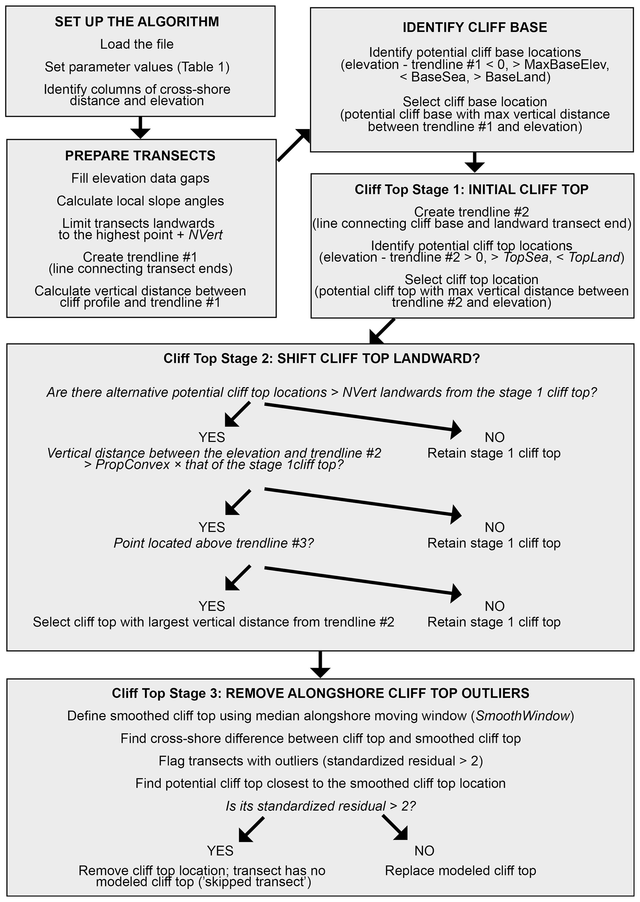
Figure 1 CliffDelineaTool workflow and the three cliff top processing stages. The calibrated parameters NVert, MaxBaseElev, BaseSea, BaseLand, TopSea, TopLand, PropConvex, SmoothWindow are defined in Table 1.

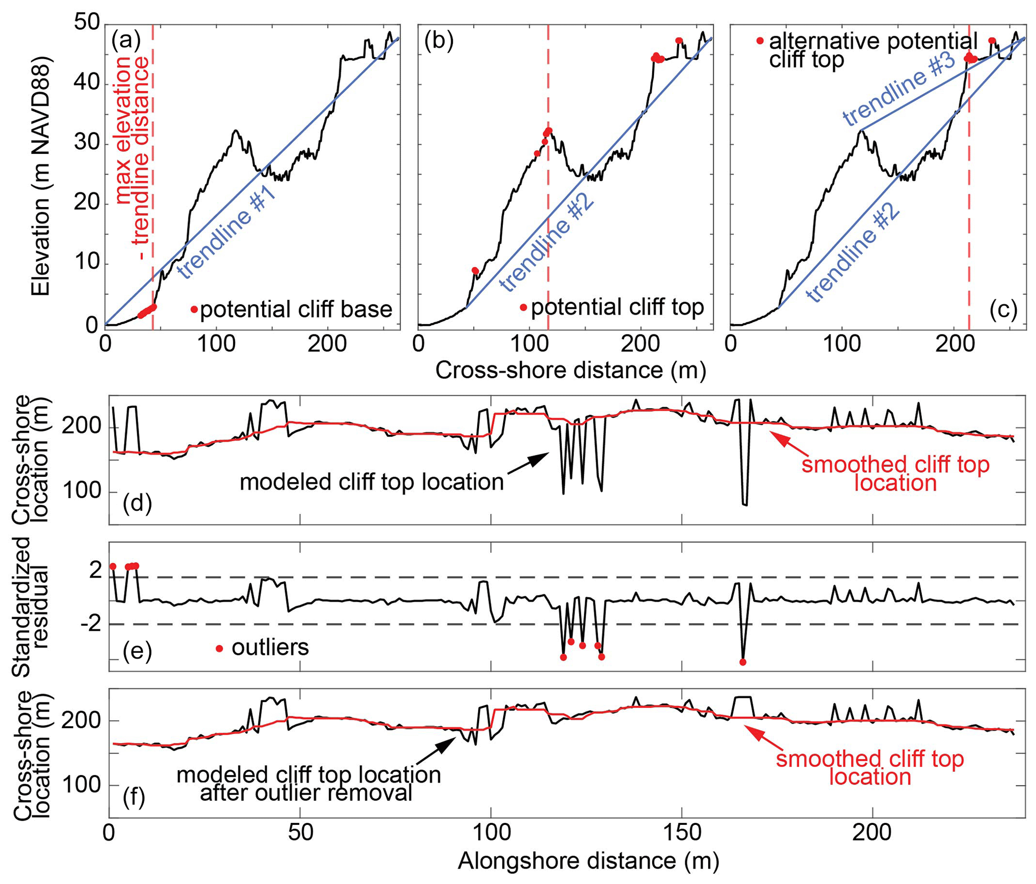
Figure 2 Example of the identification of cliff base and top positions (transect #123 of area of interest (AOI) #3; see Fig. 3c for topography and oblique photograph): (a) potential cliff base positions and the point with the largest distance from trendline #1; (b) potential cliff top positions and the point with the largest distance from trendline #2 (stage 1); (c) alternative potential cliff top positions in the case of a complex cross-shore profile, and the point with the largest distance from trendline #2 (stage 2). Identification and removal of alongshore cliff top outliers (stage 3) – alongshore distributions of (d) the stage 2 modeled and smoothed cliff top, (e) standardized residuals between the smoothed and stage 2 modeled cliff top, and (f) the stage 3 modeled cliff top with outliers removed. Note the vertical exaggeration in (a)–(c) and the horizontal exaggeration in (d)–(f).

Cliff top identification consists of three stages (Fig. 1). In stage 1, trendline #2 is created by connecting the modeled cliff base with the landward end of the transect (Fig. 2b). Potential cliff top locations are located above trendline #2 and fulfill the user-defined criteria of the minimum local seaward slope (TopSea) and maximum local landward slope (TopLand) that define local convexities. From the set of potential cliff top locations, the point with the largest vertical distance from trendline #2 is selected to represent the cliff top, following Palaseanu-Lovejoy et al. (2016) and Payo et al. (2018) (Fig. 2b). If no points along the transect fulfill the criteria, the transect is skipped and has no explicitly modeled cliff top.

In some locations with complex cliff face profiles, such as rotational landslides or mid-cliff roads, a local flattening within the cliff face may exist and cause incorrect cliff top selection. To account for these situations, in stage 2, the model checks if any alternative potential cliff top exists landwards of the initial cliff top location identified in stage 1. Alternative potential cliff top positions located closer than NVert points from the initial top are rejected to ignore points that are likely part of the same convex section. Alternative positions must also be located above trendline #3 (a line from the initial cliff top to the landward transect end, Fig. 2c), and be greater than PropConvex (values between 0 and 1) multiplied by the elevation difference between the initial cliff top and trendline #2. For example, if PropConvex = 0.5 and the initial cliff elevation is 4 m above trendline #2, potential cliff top locations must be >2 m (0.5×4 m) above trendline #2. If alternative positions exist, the initial top is relocated to the point with the largest vertical distance from trendline #2 (Fig. 2c). Otherwise, the initial cliff top is retained.

In stage 3, cliff top outliers are identified by comparing the cross-shore location to an alongshore smoothed cliff line created from the median of an alongshore moving window (SmoothWindow) (Fig. 2d). Residuals are calculated as the distance between the smoothed and modeled cross-shore locations. Transects with standardized residuals (the residual divided by the residual standard deviation) >2 are flagged as outliers (Fig. 2e) and re-examined to identify new potential cliff top locations. If the standardized residual of the potential cliff top closest to the smoothed cross-shore location is <2, it replaces the previously modeled top. Otherwise, the transect has no explicitly modeled cliff top (Fig. 2f).

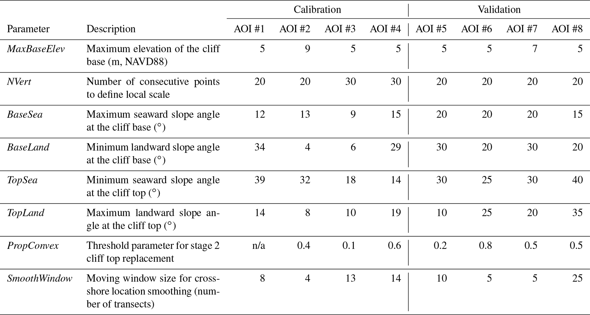
Table 1 CliffDelineaTool user-defined parameters, and values that are optimized for the calibration coastal sections (areas of interest (AOIs) #1–4) and used to validate the model (AOIs #5–8).

n/a: not applicable

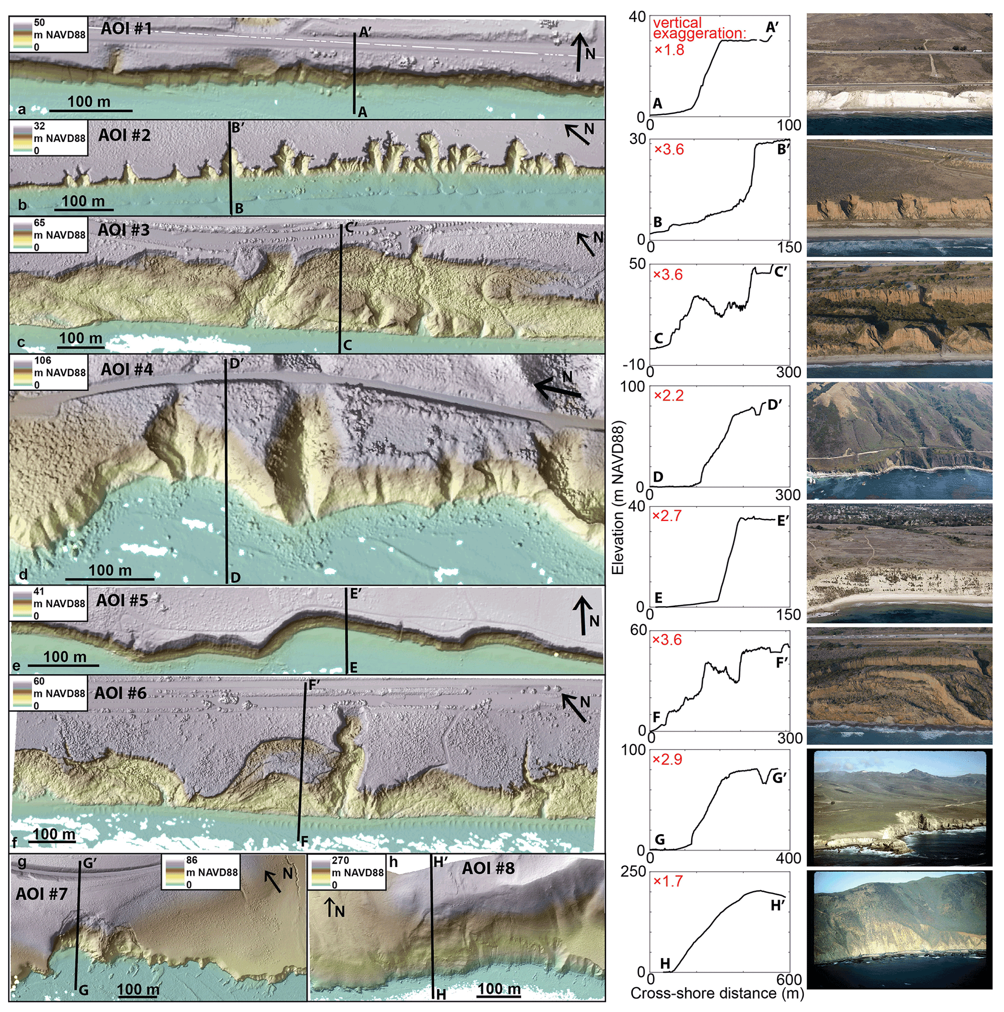
Figure 3 Areas of Interest (AOIs) used to calibrate (a–d) and validate (e–h) CliffDelineaTool. Vertical exaggeration is labeled in red for profiles. Photographs copyright © 2002–2021 Kenneth & Gabrielle Adelman, California Coastal Records Project, http://www.Californiacoastline.org (last access: 12 November 2021).

2.2 Model development

2.2.1 CliffDelineaTool calibration

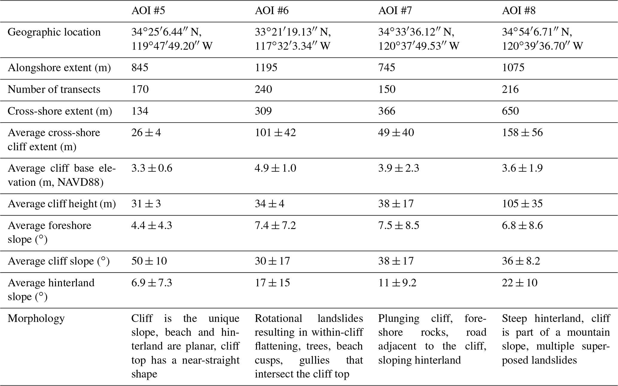
To optimize user-defined parameters (Table 1), four calibration coastal cliff sections in California (areas of interest (AOIs) #1–4) were selected that span 650–1200 m alongshore and encompass a range of geomorphic settings (Table 2; Fig. 3a–d). Topographic information for each AOI was derived from 1 m DEMs created from a 2016 airborne lidar dataset (Swirad and Young, 2021).

Table 2 Characteristics of the areas of interest (AOIs) used to calibrate CliffDelineaTool. Average values are represented as mean ± standard deviation.

Figure 4 Distributions of the local seaward and landward slopes of true cliff base and top locations for varying NVert values. Boxplots include medians (red bars), 25th (q₁) and 75th (q₃) percentiles (blue boxes), ranges excluding outliers (black whiskers), and outliers (red crosses). Outliers are defined as values greater than $q_{\mathrm{3}}+\mathrm{1.5}\times (q_{\mathrm{3}}-q_{\mathrm{1}})$ or less than $q_{\mathrm{1}}-\mathrm{1.5}\times (q_{\mathrm{3}}-q_{\mathrm{1}})$. Values in red located above the plots show the number of outliers (if >0). Gray shadow indicates the local slope distribution at the selected NVert value.

Parallel calibration transects generated with ArcGIS tools were spaced 5 m alongshore to capture mesoscale details of alongshore cliff geometry and sampled at 1 m cross-shore resolution. Points representing “true” cliff base and top locations were visually selected for each transect. The CliffDelineaTool results were compared with the distance-to-trendline method (Palaseanu-Lovejoy et al., 2016) and CliffMetrics (SAGA GIS version; Payo, 2020) using input parameters (seaward transect end points, transect length, and no transect smoothing) to match the same cross-shore transects used for CliffDelineaTool and the default vertical tolerance of 0.5. Maximum cliff base elevation (MaxBaseElev) was subjectively set to 5 m (NAVD88) for AOIs #1, #3, and #4 and to 9 m (NAVD88) for AOI #2 based on DEM inspection (Fig. 3, Table 2). The remaining seven parameters were calibrated to minimize the root mean squared error (RMS) between the true and modeled cliff base and top positions while not skipping too many transects. NVert and threshold slope angles (BaseSea, BaseLand, TopSea, and TopLand) were calibrated using the characteristics of the true cliff base and top locations. Slope angles were calculated for a range of NVert values (Table 2). Local slope angle distributions were summarized in statistical terms (Fig. 4), and outliers were defined as points greater than $q_{\mathrm{3}}+\mathrm{1.5}\times (q_{\mathrm{3}}-q_{\mathrm{1}}$) or less than $q_{\mathrm{1}}-\mathrm{1.5}\times (q_{\mathrm{3}}-q_{\mathrm{1}}$), where q₁ and q₃ are the 25th and 75th percentiles (red crosses in Fig. 4; Tukey, 1977). NVert = 20 was selected for AOIs #1–2 and NVert = 30 was selected for AOIs #3–4 to minimize the number of outliers while maintaining a relatively narrow and normal slope angle distribution. Threshold slope angles were picked as minimum or maximum values excluding outliers ($q_{\mathrm{3}}+\mathrm{1.5}\times (q_{\mathrm{3}}-q_{\mathrm{1}}$) or $q_{\mathrm{1}}-\mathrm{1.5}\times (q_{\mathrm{3}}-q_{\mathrm{1}}$); black whisker ends in Fig. 4; Table 1).

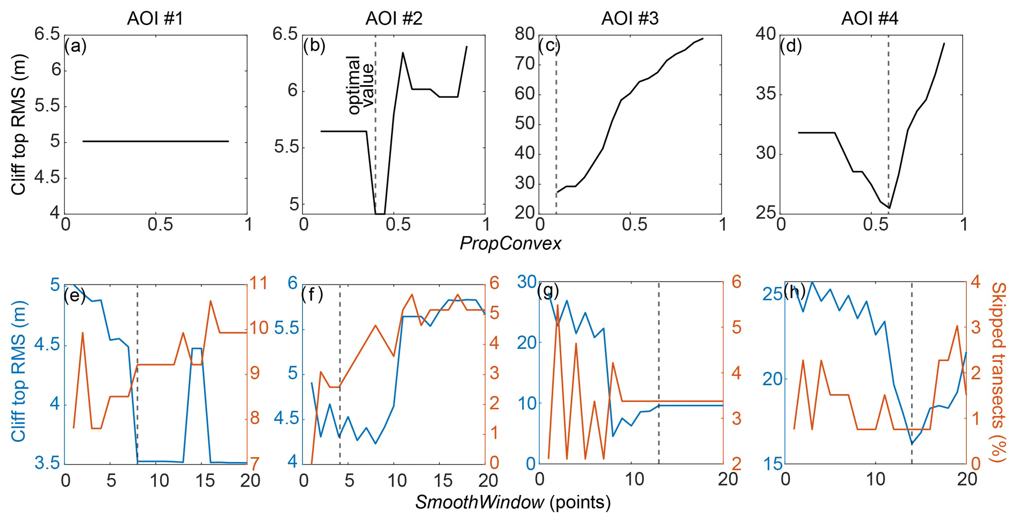
Figure 5 Calibration of PropConvex (testing from 0.1 to 0.9 at intervals of 0.05) (a–d) and SmoothWindow (testing from 1 to 20 transects) (e–h). Vertical dashed lines represent the optimal values (Table 1).

Next, CliffDelineaTool checks for false cliff tops caused by local flattening within the cliff face using PropConvex (stage 2 of the model, Fig. 1). PropConvex was calibrated by inspecting the cliff top RMS for values ranging from 0.1 to 0.9 at intervals of 0.05 (Fig. 5a–d). For the simple cliff morphology of AOI #1, introducing PropConvex did not change the modeled cliff top locations, but it did decrease the RMS for more complex AOIs #2–4 (Fig. 5a–d; Table 1). Next, cliff top outliers were identified. The optimal SmoothWindow was selected by comparing a moving window ranging from 1 to 20 alongshore transects for each AOI to minimize RMS and the number of skipped transects (Fig. 5e–h; Table 1). The modeled cliff base and top locations were converted to polylines using ArcGIS and intersected with transects to define cliff base and top locations on skipped transects. Overall, these steps improved automated cliff mapping performance for the more complex cliff sections and usually led to a lower RMS compared to the distance-to-trendline method and CliffMetrics (Table 3; Fig. 6).

Table 3 Performance of CliffDelineaTool (at various stages), the distance-to-trendline method, and CliffMetrics (Payo, 2020).

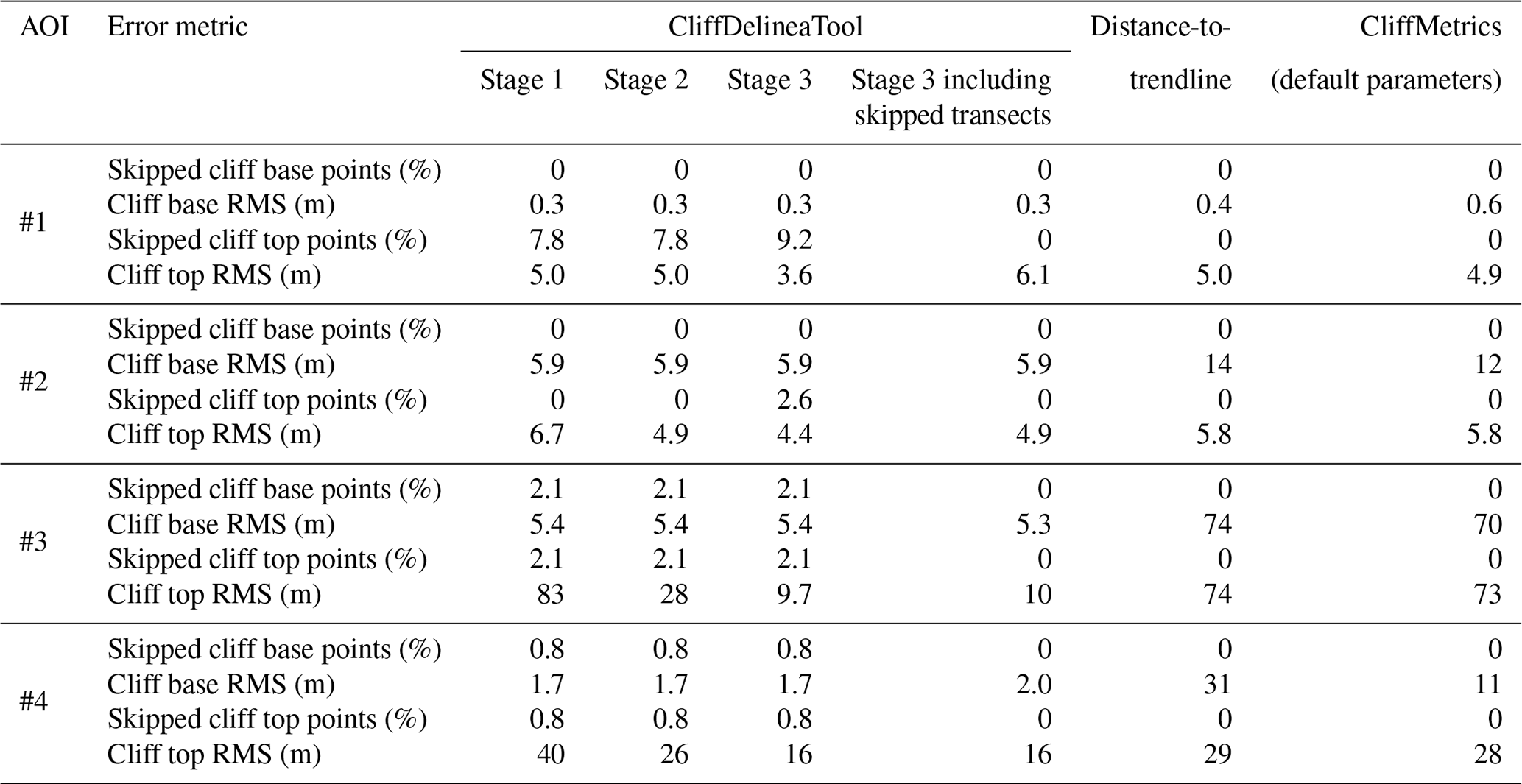
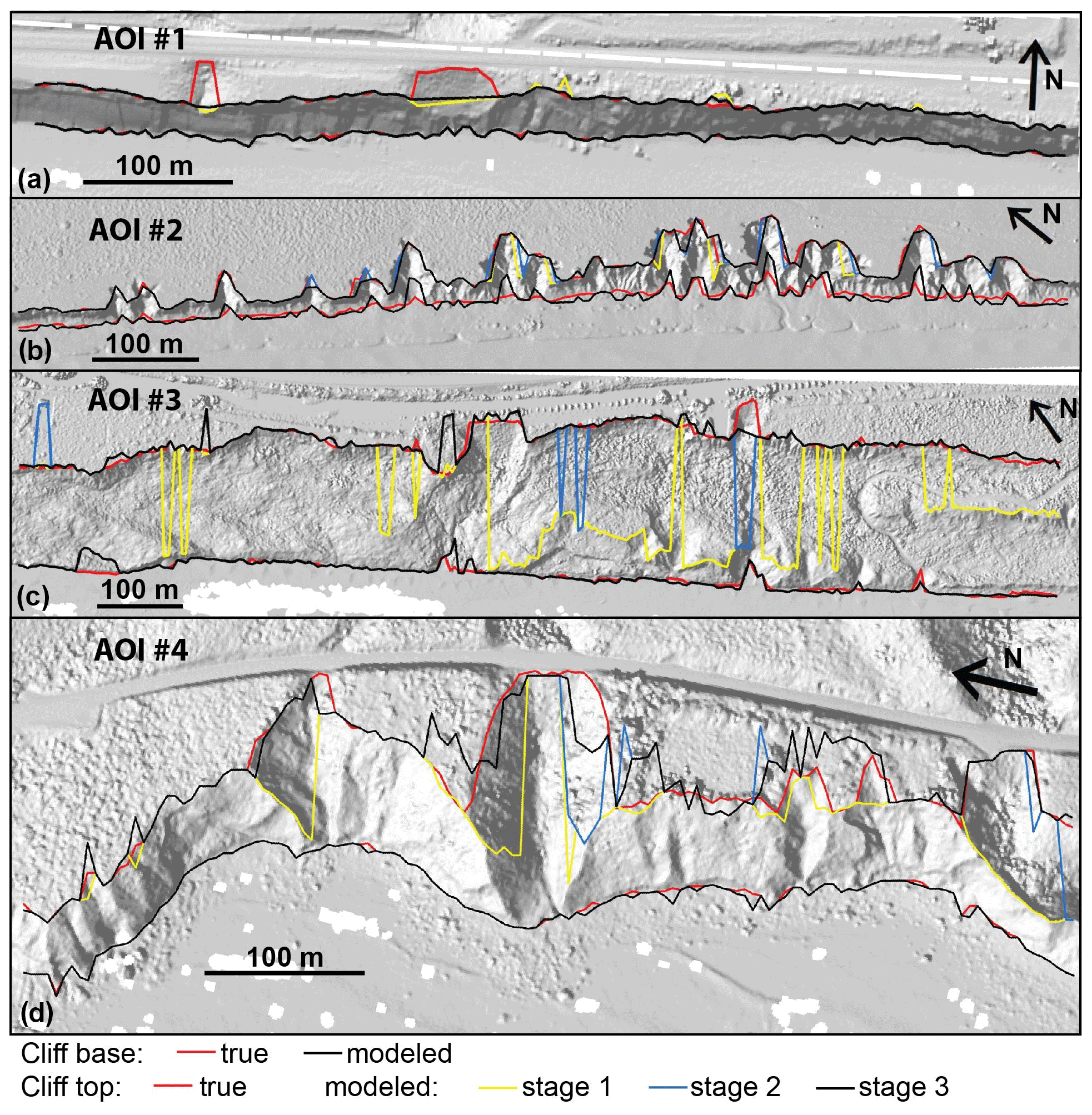
Figure 6 Locations of the cliff base and top at various stages of the CliffDelineaTool calibration.

2.2.2 CliffDelineaTool evaluation

Ten geoscientists manually digitized the cliff base and top for four different sections of the California coastline (AOIs #5–8) with diverse morphologies using 1 m resolution DEMs and hillshade maps (Table 4; Fig. 3e–h). The “true” cliff base and top positions were defined as the medians of the manually mapped positions.

Table 4 Characteristics of the areas of interest (AOIs) used to evaluate CliffDelineaTool. Average values are represented by the mean ± standard deviation.

CliffDelineaTool, the distance-to-trendline method, and CliffMetrics were applied to the four test sections (AOIs #5–8) and compared to the manually mapped cliff lines. For CliffDelineaTool, NVert was set at 20 because the test sections had the same 1 m DEM resolution as the calibration set. MaxBaseElev was set based on the average cliff base elevation (Table 4). The remaining parameter values (BaseSea, BaseLand, TopSea, TopLand, PropConvex, and SmoothWindow) were selected based on the average foreshore, cliff, and hinterland slopes (Table 4) and visual assessment of initial model runs (Table 1). The RMS between the true and modeled cliff base or top locations was used to assess model performance on all transects (including skipped transects).

Table 5 RMS between the true cliff base/top position (i.e., the median of all positions given by the 10 manual mappers) and the corresponding cliff base/top position given by a manual mapper or a modeling method.

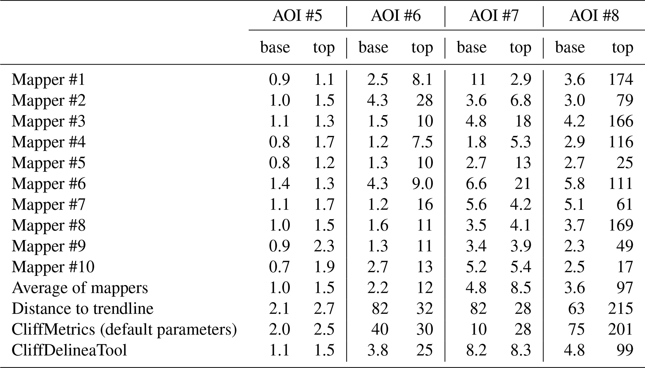
Figure 7 Cliff base and top positions for AOIs #5–8: (a, c, e, g) positions according to individual manual mappers; (b, d, f, h) true (i.e., the median from manual mapping) and modeled positions. Locations A: pre-slide cliff top position interpreted as the cliff top by mapper #2; B: cliff base placed in the hinterland by the distance-to-trendline method; C: beach cusps identified as the cliff base by the distance-to-trendline method and CliffMetrics; D: interior cliff face location selected as the cliff top by all models; E: elevated section between two landslide scars interpreted as the cliff top by two mappers; F: top of the mountain slope interpreted as the cliff top; G: cliff top placed mid-slope; H: cliff top placed in the lower part of the mountain slope.

3 Results

The consistency of the manual cliff mapping and the performance of the automated cliff mapping varied between the four evaluated AOIs. The simple cliff geometry and unambiguous location of the cliff base and top of AOI #5 resulted in a low (≤2.7 m) RMS for all mapping methods (Table 5; Fig. 7a–b). In general, cliff base locations were more consistent between manual mappers and CliffDelineaTool compared to the cliff tops. The distance-to-trendline method had a relatively high (≫10 m) cliff base RMS for all three complex AOIs (#6–8), and sometimes placed the cliff base on the upper cliff face or hinterland (B in Fig. 7d). Using default parameters, CliffMetrics generally performed better than the distance-to-trendline method, but it had a higher RMS compared to CliffDelineaTool. CliffDelineaTool (RMS = 1.1–8.2 m) and manual mapping (RMS = 0.7–11 m) gave comparable cliff base detection results. For AOI #6, the distance-to-trendline method and CliffMetrics sometimes placed the cliff base at beach cusps (C in Fig. 7d). For the complex AOIs #6–8, manual and automated cliff top positions were varied (RMS = 2.9–214 m). In AOI #6, one mapper (#2) selected the head scarp of an interior landslide as the cliff top, about 100 m from the cliff top selected by all other mappers (A in Fig. 7c). However, the models also picked sections of the landslide head scarp (D in Fig. 7d). In AOI #7, two mappers interpreted an elevated section between two separate landslide scars as the cliff top (E in Fig. 7e), whereas most other mappers and both models opted for a simpler cliff top shape (Fig. 7e and f). The cliff top position was most diverse for AOI #8, with mappers' interpretations ranging from the top of the coastal mountain slope (F in Fig. 7g) to mid-slope (G in Fig. 7g) and tops of interior cliff face landslide scars (H in Fig. 7g). CliffDelineaTool gave inconsistent results, while the distance-to-trendline method and CliffMetrics placed the cliff top at the top of the mountain slope (Fig. 7h).

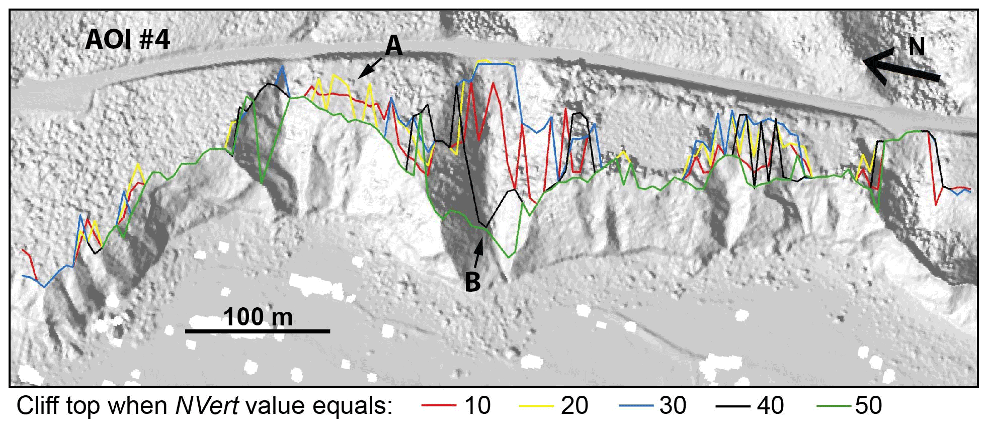
Figure 8 Location of the stage 2 cliff top after optimizing all parameters for NVert ranging from 10 to 50. Location A: vegetation interpreted as the cliff top for model runs with low NVert values. Location B: high NVert values can inhibit correct stage 2 cliff top replacement to locations further landward.

4 Discussion

Acceptable model results depend on the purpose of cliff delineation. At the scale and resolution considered here, the model generally provided comparable results to manual mapping for diverse cliff morphologies. Model performance generally correlates with the amount of inconsistency between manual mappers, which is related to the cliff complexity. For example, in the complex AOI #8, the mean manual mapper and CliffDelineaTool RMSs were both high (97 and 99 m, respectively). Conversely, for the simple AOI #5, the manual mapper and CliffDelineaTool RMSs were both low (1.5 m for both). The present model does not resolve the situation where a transect crosses the cliff top multiple times, and typically places the cliff top at the seawardmost crossing point (Fig. 6b). Other model application issues include occasionally selecting treetop locations for cliff top positions (Fig. 6c and d) when using non-bare-earth DEMs. Given these issues and the high RMS for complex cliff sections, we suggest that model outputs should be visually controlled (similar to Payo et al., 2018), and should not be used where the cliff top is very ambiguous, such as AOI #8 with complex tall mountain slopes.

Unlike the models of Palaseanu-Lovejoy et al. (2016) and Payo et al. (2018), CliffDelineaTool does not generate transects. For this study, simple cross-shore transects with 5 m alongshore spacing were defined manually for each AOI. The relatively short AOI alongshore sections permitted the use of parallel transects (Swirad, 2021). However, for longer, more complex cliff sections, varying the transect orientation will improve results and could be generated with CliffMetrics (Payo et al., 2018).

We compared CliffDelineaTool to the distance-to-trendline method, which forms the basis of iBluff (Palaseanu-Lovejoy, 2021) and CliffMetrics (Payo et al., 2018). However, iBluff and CliffMetrics both include additional steps to improve results and correct erroneous cliff base and top positions. iBluff uses manual transect shortening during preprocessing, and outlier removal with a smoothing window, similar to CliffDelineaTool. CliffMetrics uses manual quality control and iterative parameter selection (Payo et al., 2018). The CliffMetrics results presented here used default parameters and predefined transects to provide a direct comparison to CliffDelineaTool. However, one of the strengths of CliffMetrics is the ability to quickly iterate the parameter setup. Therefore, the results could be improved by using iterative parameter selection and varying the transect length and orientation.

For best performance, CliffDelineaTool should be calibrated to the user study section. The input parameters have a varied impact on model performance (Fig. 6). MaxBaseElev is easily selected using a slightly conservative cliff base elevation estimated from the general site settings. The optimal NVert parameter depends on DEM resolution and cross-shore cliff extent. Calibration showed that, in general, the greater the NVert value, the narrower the distribution of the four threshold slopes (BaseSea, BaseLand, TopSea, and TopLand) and the higher the number of outliers. That relationship holds until an NVert value (30 for AOI #1, 40 for #3, and 70 for #4, Fig. 4) over which the q₁−q₃ box becomes very wide or the distribution is dominated by outliers. Figure 8 shows the cliff top optimized for NVert values of 10, 20, 30, 40, and 50 for AOI #4. It suggests that during stage 2, a low NVert value can cause an incorrect cliff top section due to minor protruding features such as vegetation (A in Fig. 8), while a higher value can inhibit correct stage 2 cliff top replacement (B in Fig. 8). A TopLand of 10–20^∘ is generally appropriate when the hinterland is planar or gently sloping but should be increased for cliffs with steeper inland areas. BaseSea and BaseLand are important for proper cliff base placement in coastal sections with back beach cusps and landslide deposits. The SmoothWindow parameter depends on the alongshore complexity of the coast, the bay/headland sequence spacing, and their relation to transect spacing. Model results are sensitive to TopSea, PropConvex, and SmoothWindow, and testing various values on short sections of the study area with visual inspection can help identify optimal values (Fig. 6).

Two previous studies have successfully used parts of CliffDelineaTool. Swirad and Young (2021) used a modified version of CliffDelineaTool to automate the mapping of cliff base and top positions along the California coast (1646 km). The modified version did not include stage 2 (shifting the cliff top landwards for within-cliff flattening areas) and stage 3 (removal of outliers), but it did include a Laplacian topographic filter (Richter et al., 2013). The automated results were visually inspected, and some (10 % of the cliff base and 29 % of the cliff top positions) required manual modification to correct positions. Young et al. (2021) used the present CliffDelineaTool model to identify the cliff base in 155 0.25 m-resolution DEMs along a 2.5 km coastal section with 1 m alongshore transect spacing. Quality control showed that cliff base misplacement was negligible, while the total processing time was ∼30 min (Young et al., 2021). These studies demonstrate the tool's applicability for both large space and time datasets, and over a range of DEM resolutions.

5 Conclusions

Building on previous studies, we developed a new algorithm (CliffDelineaTool) to delineate coastal cliffs from DEMs. The model identifies cliff base and top positions along cross-shore transects using elevation and slope characteristics. It considers complex cliff morphologies and removes alongshore cliff top outliers. CliffDelineaTool provides results comparable to manual mapping and improves cliff base and top identification for complex cross-profiles. The automated results have known errors and should be inspected visually. The method has been applied successfully to two large datasets (Swirad and Young, 2021; Young et al., 2021), greatly reducing processing time. With calibration and quality control, CliffDelineaTool can be used in a wide variety of coastal settings, facilitating a range of scientific and managerial applications, but it has limited application where the cliff top is ambiguous.