the Creative Commons Attribution 4.0 License.
the Creative Commons Attribution 4.0 License.
 | 17 Feb 2022
A circulation-based performance atlas of the CMIP5 and 6 models for regional climate studies in the Northern Hemisphere mid-to-high latitudes
Global climate models are a keystone of modern climate research. In most applications relevant for decision making, they are assumed to provide a plausible range of possible future climate states. However, these models have not been originally developed to reproduce the regional-scale climate, which is where information is needed in practice. To overcome this dilemma, two general efforts have been made since their introduction in the late 1960s. First, the models themselves have been steadily improved in terms of physical and chemical processes, parametrization schemes, resolution and implemented climate system components, giving rise to the term “Earth system model”. Second, the global models' output has been refined at the regional scale using limited area models or statistical methods in what is known as dynamical or statistical downscaling. For both approaches, however, it is difficult to correct errors resulting from a wrong representation of the large-scale circulation in the global model. Dynamical downscaling also has a high computational demand and thus cannot be applied to all available global models in practice. On this background, there is an ongoing debate in the downscaling community on whether to thrive away from the “model democracy” paradigm towards a careful selection strategy based on the global models' capacity to reproduce key aspects of the observed climate. The present study attempts to be useful for such a selection by providing a performance assessment of the historical global model experiments from CMIP5 and 6 based on recurring regional atmospheric circulation patterns, as defined by the Jenkinson–Collison approach. The latest model generation (CMIP6) is found to perform better on average, which can be partly explained by a moderately strong statistical relationship between performance and horizontal resolution in the atmosphere. A few models rank favourably over almost the entire Northern Hemisphere mid-to-high latitudes. Internal model variability only has a small influence on the model ranks. Reanalysis uncertainty is an issue in Greenland and the surrounding seas, the southwestern United States and the Gobi Desert but is otherwise generally negligible. Along the study, the prescribed and interactively simulated climate system components are identified for each applied coupled model configuration and a simple codification system is introduced to describe model complexity in this sense.
- Article
(42792 KB) - Full-text XML
-
Supplement
(12089 KB) - BibTeX
- EndNote


General circulation models (GCMs) are numerical models capable of simulating the temporal evolution of the global atmosphere or ocean. This is done by integrating the equations describing the conservation laws of physics along time as a function of varying forcing agents, starting with some initial conditions (AMS, 2020). If run in standalone mode, an atmospheric general circulation model (AGCM) is coupled with an indispensable land-surface model (LSM) only, whilst the remaining components of the extended climate system (also called “realms” in the nomenclature of the Earth System Grid Federation), including ocean, sea-ice and vegetation dynamics (depending on the model, also atmospheric chemistry, aerosols, ocean biogeochemistry and ice-sheet dynamics), are read in from static datasets instead of being simulated online (Gates, 1992; Eyring et al., 2016; Waliser et al., 2020). In these “atmosphere-only” experiments, the number of coupled realms is kept at a minimum in order to either isolate the sole atmospheric response to temporal variations in the aforementioned other components (Schubert et al., 2016; Brands, 2017; Deser et al., 2017) or to put all available computational resources into the proper simulation of the atmosphere, e.g. by augmenting the spatial and temporal resolution (Haarsma et al., 2016). This kind of experiment is traditionally hosted by the Atmospheric Model Intercomparison Project (AMIP) (Gates, 1992).
In a global climate model, interactions and feedbacks between the aforementioned realms are explicitly taken into account by coupling the AGCM and LSM with other component models. In the “ocean–atmosphere” configuration (AOGCM, for atmosphere–ocean general circulation model), the AGCM plus an LSM are coupled with an ocean general circulation model (OGCM) and a sea-ice model. Further model components representing the effects of vegetation, atmospheric chemistry, aerosols, ocean biogeochemistry and ice-sheet dynamics are then optionally included with the final aim to reach a representation of the climate system as comprehensive as possible with the current level of knowledge and available computational resources. However, due to the vast number of nonlinearly interacting processes, coupled climate models are prone to many error sources and model uncertainties, making it difficult to directly compare the simulated climate with the observed one (Watanabe et al., 2011; Yukimoto et al., 2011).
Since coupled model experiments are the best known approximation to the real climate system, they constitute the starting point of most climate change impact, attribution and mitigation studies. For use in impact studies, the coarse-resolution GCM output is usually downscaled with statistical or numerical models (Maraun et al., 2010; Jacob et al., 2014; Gutiérrez et al., 2013; San-Martín et al., 2016) or a combination thereof (Turco et al., 2011), in order to provide information on the regional to local scale where it can then be used for decision making.
Now while downscaling methods are able to imprint the effects of the local climate factors on the coarse-resolution GCM, the correction of errors inherited from a wrong representation of the large-scale atmospheric circulation is challenging (Prein et al., 2019). A physically consistent way to circumvent this “circulation error” is choosing a GCM (or group of GCMs) capable of realistically simulating the climatological statistics of the regional-scale circulation. This is why careful GCM selection for long has been the subject of any careful downscaling approach applied in a climate change context (Hulme et al., 1993; Mearns et al., 2003; Brands et al., 2013; Fernandez-Granja et al., 2021). However, due to the availability of many GCMs from many different groups, this idea has been partly replaced by the “model democracy” paradigm discussed, e.g. in Knutti et al. (2017), where as many GCMs as possible are applied irrespective of their performance in present-day conditions (Jacob et al., 2014). In the recent past, the importance of careful model selection has been re-emphasized in the context of bias correction, which can be considered a special case of statistical downscaling (Maraun et al., 2017). It should be also remembered that GCMs by definition were not developed to realistically represent regional-scale climate features (Grotch and MacCracken, 1991; Palmer and Stevens, 2019) and that they have been pressed into this role during the last 3 decades due to the ever-increasing demand for climate information on this scale. Hence, finding a GCM capable of reproducing the regional atmospheric circulation in a systematic way, i.e. in many regions of the world, would be anything but expected.
In the present study, a total of 128 historical runs from 56 distinct GCMs (or GCM versions) of the fifth and sixth phases of the Coupled Model Intercomparison Project (CMIP5 and 6) are evaluated in terms of their capability to represent the present-day climatology of the regional atmospheric circulation as represented by the frequency of the 27 circulation types proposed by Lamb (1972). Based on the proposal in Jones et al. (2013) that this scheme can in principle be applied within a latitudinal band from 30∘ to 70∘ N, it is here used with a sliding coordinate system (Otero et al., 2017) running along the grid boxes of a 2.5∘ latitude–longitude grid covering the entire Northern Hemisphere mid-to-high latitudes.
In Sects. 2 and 3, the applied data, methods and software are described. In Sect. 4, the results of an overall model performance analysis including all 27 circulation types are presented. First, those regions are identified where reanalysis uncertainty might compromise the results of any GCM performance assessment based on a single reanalysis. Then, an atlas of overall model performance is provided for each participating model (Sect. 4.1 to 4.8). The present article file focuses on the evaluation with respect to ERA-Interim, complemented by pointing out deviations from the evaluation with respect to the Japanese 55-year Reanalysis (JRA-55) in the three relevant regions in the running text. The full atlas of the evaluation against JRA-55 is provided in the Supplement to this study (see “figs-refjra55” folder therein). In Sect. 4.9, the atlas is summarized, associations between the models' performance and their resolution in the atmosphere and ocean are drawn, and the role of internal model variability is assessed with 72 additional historical runs from a subgroup of 13 models. Finally, the results of a specific model performance evaluation for each circulation type are provided in Sect. 5, followed by a discussion of the main results and some concluding remarks in Sect. 6. For the sake of simplicity, the model performance atlas is grouped by the geographical location of the coupled models' coordinating institutions, having in mind that most model developments are actually international or even transcontinental collaborating efforts.
The study resides on 6-hourly instantaneous sea-level pressure (SLP) model data retrieved from the Earth System Grid Federation (ESGF) data portals (e.g. https://esgf-data.dkrz.de/projects/esgf-dkrz/, last access: 11 February 2022), whose digital object identifiers (DOIs) can be obtained following the references in Table 1. These model runs are evaluated against reanalysis data from ECMWF ERA-Interim (Dee et al., 2011) (https://apps.ecmwf.int/datasets/data/interim-full-daily/levtype=sfc/, last access: 11 February 2022) and the Japan Meteorological Agency (JMA) JRA-55 (Kobayashi et al., 2015) (https://rda.ucar.edu/datasets/ds628.0/last access: 11 February 2022, https://doi.org/10.5065/D6HH6H41, Japan Meteorological Agency, 2013). In a first step, and in order to compare as many distinct models as possible, a single historical run was downloaded for each model for which the aforementioned data were available for the 1979–2005 period. If several historical integrations for a given model version were available, then the first member was chosen. In Sect. 4.9, it will be shown that the selection of alternative members from a given ensemble does not lead to substantial changes in the results. Out of the 31 models used in CMIP6, 26 were run with the “f1”, four with the “f2” and one with the “f3” forcing datasets (Eyring et al., 2016) (see Table 1). Not only version pairs from CMIP5 to CMIP6 are considered but also model versions either not having a predecessor in CMIP5 or a successor in CMIP6. In the most favourable case, two versions of a given model are available for both CMIP5 and 6: a higher-resolution setup considering fewer realms (the AOGCM configuration), complemented by a more complex setup including more component models, usually run with a lower resolution than the AOGCM version.
Bi et al. (2013)Bi et al. (2013)Bi et al. (2020)Ziehn et al. (2020)Semmler et al. (2020)Wu et al. (2013, 2014)Wu et al. (2019)Chylek et al. (2011)Gent et al. (2011)Scoccimarro et al. (2011)Cherchi et al. (2019)Cherchi et al. (2019)Voldoire et al. (2013)Voldoire et al. (2019)Voldoire et al. (2019)Séférian et al. (2019)Collier et al. (2011)Hazeleger et al. (2011)Döscher et al. (2021)Döscher et al. (2021)Döscher et al. (2021)Döscher et al. (2021)Döscher et al. (2021)Li et al. (2013)Li et al. (2020)Griffies et al. (2011)Held et al. (2019)Schmidt et al. (2014)Schmidt et al. (2014)Kelley et al. (2020)Collins et al. (2011)Collins et al. (2011)Roberts et al. (2019)Swapna et al. (2015)Volodin et al. (2010)Dufresne et al. (2013)Dufresne et al. (2013)Boucher et al. (2020)Pak et al. (2021)Watanabe et al. (2010)Watanabe et al. (2011)Tatebe et al. (2019)Hajima et al. (2020)Giorgetta et al. (2013)Giorgetta et al. (2013)Mauritsen et al. (2019)Müller et al. (2018)Mauritsen et al. (2019)Yukimoto et al. (2011)Yukimoto et al. (2019)Cao et al. (2018)Bentsen et al. (2013)Seland et al. (2020)Seland et al. (2020)Park et al. (2019)Lee et al. (2020)Table 1Overview of the applied model experiments, including the abbreviations of the coupled models and their atmosphere and ocean components, their resolution expressed as number of longitudinal × latitudinal grid boxes (gb), number of vertical model levels (lv), run identifiers (complemented by Fig. 12 for more than one run), reference articles, model complexity codes as defined in Sect. 3.3, reanalysis affinity and median mean absolute error (MAE) with respect to ERA-Interim; Gr indicates Gaussian reduced grid; the ocean grids are described in Appendix A.
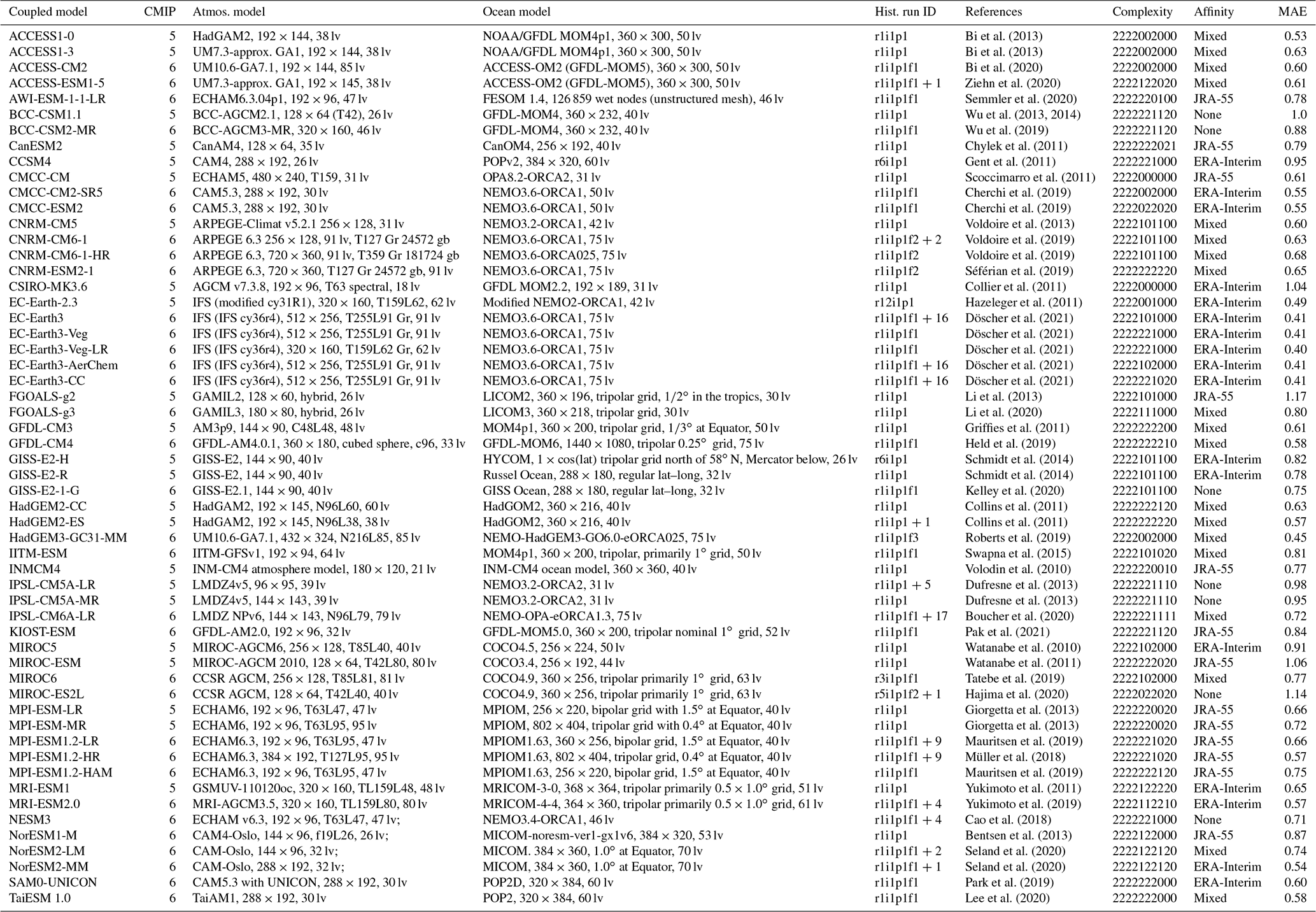
An overview of the 56 applied model versions is provide in Table 1. The table provides information about the component AGCMs and OGCMs, their horizontal and vertical resolution, run specifications and complexity codes described in Sect. 3.3.
For 13 selected models (ACCESS-ESM1, CNRM-CM6-1, HadGEM2-ES, EC-Earth3, IPSL-CM5A-LR, IPSL-CM6A-LR, MIROC-ES2L, MPI-ESM1-2-LR, MPI-ESM1-2-HR, MRI-ESM2, NorESM2-LM, NorESM2-MM, NESM3), a total of 72 additional historical integrations (between 1 and 17 additional runs per model) were retrieved from the respective ensembles in order to assess the effects of internal model variability. By definition of the experimental protocol followed in CMIP, ensemble spread relies on initialization from distinct starting dates of the corresponding pre-industrial control runs – or similar, shorter runs as, e.g. indicated in Roberts et al. (2019) – i.e. on “initial conditions uncertainty” (Stainforth et al., 2007).
3.1 Lamb weather types
The classification scheme used here is based on Hubert Horace Lamb's practical experience when grouping daily instantaneous SLP maps for the British Isles and interpreting their relationships with the regional weather (Lamb, 1972). This subjective classification scheme contained 27 classes and was brought to an automated and objective approach by Jenkinson and Collison (1977) in what is known as the “Lamb circulation type” or “Lamb weather type” (LWT) approach (Jones et al., 1993, 2013).

Figure 1Illustrative example for the usage of the Lamb weather type approach over the central Iberian Peninsula. The coordinate system configured for this region and a subset of 14 types as well as their relative occurrence frequencies are shown. Note that in the present study, all 27 types originally defined in Lamb (1972) are being used. The figure is taken from Brands et al. (2014), courtesy of John Wiley and Sons, Inc.
The spatial extension of the 16-point coordinate system defining this classification is 30 longitudes × 20 latitudes with longitudinal and latitudinal increments of 10 and 5∘, respectively (see Fig. 1 for an example over the Iberian Peninsula). The following numbers are place holders of instantaneous SLP values (in hPa) at the corresponding location p (from west to east and north to south):
and the variables needed for classification are defined as follows:
where , , , and d=0.5(cos (ϕ)2); ϕ is the central latitude and δϕ is the latitudinal distance.
The 27 classes are then defined following Jones et al. (1993) and Jones et al. (2013):
-
The direction of flow is . Add 180∘ if W is positive. The appropriate direction is calculated on an eight-point compass allowing 45∘ per sector. Thus, as an example, a westerly flow would occur between 247.5 and 292.5∘.
-
If is less than F, then the flow is essentially straight and corresponds to one of the eight purely directional types defined by Lamb: northeast (NE), east (E), SE, S, SW, W, NW, N.
-
If is greater than 2F, then the pattern is either strongly cyclonic (for Z>0) or anticyclonic (for Z<0), which corresponds to Lamb's pure cyclonic (PC) or anticyclonic type (PA), respectively.
-
If lies between F and 2F, then the flow is partly directional and either cyclonic or anticyclonic, corresponding to Lamb's hybrid types. There are eight directional–anticyclonic types (anticyclonic northeast (ANE), anticyclonic east (AE), ASE, AS, ASW, AW, ANW, AN and another eight directional-cyclonic types (cyclonic northeast (CNE), cyclonic east (CE), CSE, CS, CSW, CW, CWN, CN.
-
If F is less than 6 and is less than 6, there is light indeterminate flow corresponding to Lamb's unclassified type U. The choice of 6 is dependent on the grid spacing and would need tuning if used with a finer grid resolution.
An illustrative example for the results obtained from this scheme is provided in Fig. 1 for the case of the central Iberian Peninsula. Shown is the coordinate system and the composite SLP maps for a subset of 14 LWTs, as well as the respective relative occurrence frequencies, taken from Brands et al. (2014) (courtesy of John Wiley and Sons, Inc.).
Particularly since the 1990s, this classification scheme has been used in many other regions of the Northern Hemisphere (NH) mid-to-high latitudes (Trigo and DaCamara, 2000; Spellman, 2016; Wang et al., 2017; Soares et al., 2019). Since the LWTs are closely related to the local-scale variability of virtually all meteorological and many other environmental variables (Lorenzo et al., 2008; Wilby and Quinn, 2013), they constitute an overarching concept to verify GCM performance in present climate conditions and have been used so in a number of studies (Hulme et al., 1993; Osborn et al., 1999; Otero et al., 2017).
Here, for each model run and the ERA-Interim or JRA-55 reanalysis, the 6-hourly instantaneous SLP data from 1 January 1979 to 31 December 2005 are bilinearly interpolated to a regular latitude–longitude grid with a resolution of 2.5∘. Then, the Lamb classification scheme is applied for each time instance and grid box, using a sliding coordinate system whose centre is displaced from one grid box to another in a loop recurring all latitudes and longitudes of the aforementioned grid within a band from 35 to 70∘ N. Note that the geographical domain is cut at 35∘ N (and not at 30∘ N) because the various available reanalyses are known to produce comparatively large differences in their estimates for the “true” atmosphere when approaching the tropics (Brands et al., 2012, 2013). Also, since some models do not apply the Gregorian calendar but work with 365 or even 360 d per year, relative instead of absolute LWT frequencies are considered. Further, since HadGEM2-CC and HadGEM2-ES lack SLP data for December 2005, this month is equally dropped from ERA-Interim or JRA-55 when compared with these models.
As mentioned above, the LWT approach has been successfully applied for many climatic regimes of the NH, including the extremely continental climate of central Asia (Wang et al., 2017), which confirms the proposal made in Jones et al. (2013) that the method in principle can be applied in a latitudinal band from 30 to 70∘ N. Here, a criterion is introduced to explicitly test this assumption. Namely, it is established that the LWT method should not be used at a given grid box if the relative frequency for any of the 27 types is lower than 0.1 % (i.e. 1.5 annual occurrences on average). Note that, already in its original formulation for the British Isles, some LWTs were found to occur with relative frequencies as small as 0.47 % (Perry and Mayes, 1998). This is why the 0.1 % threshold seems reasonable in the present study. If at a given grid box this criterion is not met in the LWT catalogue derived from ERA-Interim or alternatively JRA-55, then this grid box does not participate in the evaluation.
3.2 Applied GCM performance measures
To measure GCM performance, the mean absolute error (MAE) of the n=27 relative LWT frequencies obtained from a given model (m) with respect to those obtained from the reanalysis (o) is calculated at a given grid box:
The MAE is then used to rank the 56 distinct models at this grid box. The lower the MAE, the lower the rank and the better the model. After repeating this method for each grid box of the NH, both the MAE values and ranks are plotted for each individual model on a polar stereographic projection.
In addition to the MAE measuring overall performance, the specific model performance for each LWT is also assessed. This is done because, by definition of the MAE, errors occurring in the more frequent LWTs are penalized more than those occurring in the rare LWTs. Hence, a low MAE might mask errors in the least frequent LWTs. For a LWT-specific evaluation, the simulated frequency map for a given LWT and model are compared with the corresponding map from the reanalysis by means of the Taylor diagram (Taylor, 2001). This diagram compares the spatial correspondence of the simulated and observed (or “quasi-observed” since reanalysis data are used) frequency patterns by means of three complementary statistics. These are the Pearson correlation coefficient (r), the standard deviation ratio (ratio ), with σm and σo being the standard deviation of modelled and observed frequency patterns, and the normalized centred root-mean-square error (CRMSE):
with n=2016 grid boxes covering the NH mid-to-high latitudes and cm and co the modelled and observed frequency patterns after subtracting their own mean value (i.e. both the minuend and subtrahend are anomaly fields; “c” refers to centred). Normalization enables comparison with other studies using the same method.
3.3 Model complexity in terms of considered climate system components
In addition to the model performance assessment, a straightforward approach is followed to describe the complexity of the coupled model configurations in terms of considered climate system components. The following 10 components are taken into account: (1) atmosphere, (2) land surface, (3) ocean, (4) sea ice, (5) vegetation properties, (6) terrestrial carbon-cycle processes, (7) aerosols, (8) atmospheric chemistry, (9) ocean biogeochemistry and (10) ice-sheet dynamics. An integer is assigned to each of these components depending on whether it is not taken into account at all (0), represented by an interactive model feeding back on at least one other component (2) or anything in between (1) including prescription from external files, semi-interactive approaches or components simulated online but without any feedback on other components.
As an example, MRI-ESM's complexity code is 2222122220, indicating interactive atmosphere, land-surface, ocean and sea-ice models, prescribed vegetation properties, interactive terrestrial carbon-cycle, aerosol, atmospheric chemistry and ocean biogeochemistry models, and no representation of ice-sheet dynamics. For each of the 56 participating coupled model configurations, the reference article(s) and source attributes inside the NetCDF files from ESGF were assessed in order to obtain an initial “best-guess” complexity code. This code was then sent by e-mail to the respective modelling group for confirmation or correction (see the Acknowledgements). Out of the 19 groups contacted within this survey, 18 confirmed or corrected the code and 1 did not answer. Among the 18 groups providing feedback, a single scientist from one group was not sure whether the proposed method is suitable to measure model complexity but did not reject it either. In light of the many participating scientists (up to three individuals per group were contacted to enhance the probability of a response), this is considered favourable feedback. The final codes are listed in Table 1, column 7. The sum of the integers is here taken as an estimator for the complexity of the coupled model configuration and is referred to as “complexity score” in the forthcoming text. In the light of various available definitions for the term “Earth system model” (Collins et al., 2011; Yukimoto et al., 2011; Jones, 2020), this is a flexible approach used as a starting point for further specifications in the future.
Note that the here-defined complexity score only measures the number and treatment of the climate system components considered by a given coupled model configuration. It does not measure the comprehensiveness of the individual component models, nor the coupling frequency or treatment of the forcing datasets, among others. The score should thus be interpreted as an overarching and a priori indicator of climate system representativity and by no means can compete with in-depth studies treating model comprehensiveness for single climate system components (Séférian et al., 2020). For further details on the 56 coupled model configurations considered here, the interested reader is referred to the reference articles listed in Table 1, complemented by further citations in Sect. 4.
Along with other metadata including the names and versions of all component models and couplers, resolution details of the AGCMs and OGCMs and others, the complexity codes have been stored in the Python function get_historical_metadata.py contained in https://doi.org/10.5281/zenodo.4555367 (Brands, 2022).
3.4 Applied Python packages
The coding to the present study relies on the Python v2.7.13 packages xarray v0.9.1 written by Hoyer and Hamman (2017) (https://doi.org/10.5281/zenodo.264282, Hoyer et al., 2017), NumPy v1.11.3 written by Harris et al. (2020) (https://github.com/numpy/numpy, last access: 11 February 2022), Pandas v0.19.2 written by McKinney (2010) (https://doi.org/10.5281/zenodo.3509134, Reback et al., 2022) and SciPy v0.18.11 written by Virtanen et al. (2020) (https://doi.org/10.5281/zenodo.154391, Virtanen et al., 2016); here used for I/O tasks and statistical analyses. The Matplotlib v2.0.0 package written by Hunter (2007) (https://doi.org/10.5281/zenodo.248351, Droettboom et al., 2017), as well as the Basemap v1.0.7 toolkit (https://github.com/matplotlib/basemap, last access: 11 February 2022) are applied for plotting and the functions written by Gourgue (2020) (https://doi.org/10.5281/zenodo.3715535, Gourgue, 2020) for generating Taylor diagrams.
In Fig. 2, the MAE of JRA-55 with respect to ERA-Interim is mapped (panel a), complemented by the corresponding rank within the multi-model ensemble plus JRA-55 (panel b). In the ideal case, the MAE for JRA-55 is lower than for any of the 56 CMIP models, which means that the alternative reanalysis ranks first and that a change in the reference reanalysis does not influence the model ranking. This result is indeed obtained for a large fraction of the NH. However, in the Gobi Desert, Greenland and the surrounding seas, and particularly in the southwestern United States, substantial differences are found between the two reanalyses. Since different reanalyses from roughly the same generation are in principle equally representative of the “truth” (Sterl, 2004), the models are here evaluated twice in order to obtain a robust picture of their performance. In the present article file, the evaluation results with respect to ERA-Interim are mapped and deviations from the evaluation against JRA-55 in the three relevant regions are pointed out in the text. In the remaining regions, reanalysis uncertainty plays a minor role. Nevertheless, for the sake of completeness, the full atlas of the JRA-55-based evaluation was added to the Supplement to this study. For a quick overview of the results, Table 1 indicates whether a given model closer agrees with ERA-Interim or JRA-55 in the three sensitive regions. In the following, this is referred to as “reanalysis affinity”.
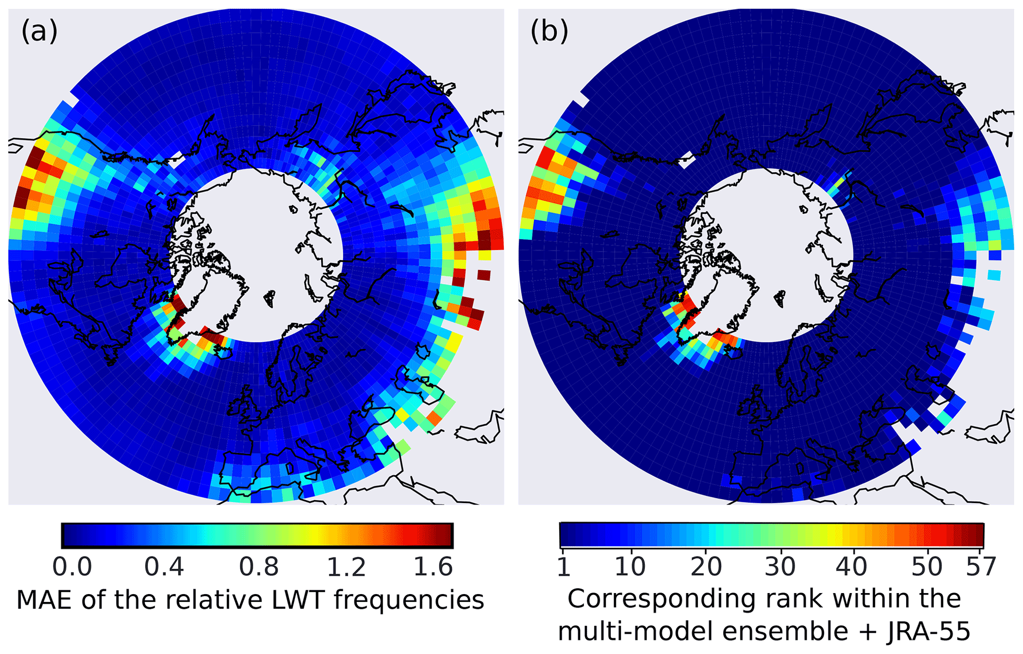
Figure 2Mean absolute error of the relative Lamb weather type frequencies from JRA-55 with respect to ERA-Interim (a), as well as the respective rank within the multi-model ensemble plus JRA-55 (b). The lower the rank, the lower the MAE and the closer the agreement between JRA-55 and ERA-Interim.
Figure 2 also shows that the LWT usage criterion defined in Sect. 3.1 is met almost everywhere in the domain, except in the high-mountain areas of central Asia (grey areas within the performance maps indicate that the criterion is not met). This region is governed by the monsoon rather than the turnover of dynamic low- and high-pressure systems the LWT approach was developed for. It is thus justified to use the approach over such a large domain.
Grouped by their geographical origin, Sects. 4.1 to 4.8 describe the composition of the 56 participating coupled models in terms of their atmosphere, land-surface, ocean and sea-ice models in order to make clear whether there are shared components between nominally different models that might explain common error structures. The names of all other component models are documented in the Python function get_historical_metadata.py contained in https://doi.org/10.5281/zenodo.4555367 (Brands, 2022). Then, the regional error and ranking details are provided. In Sect. 4.9, these results are summarized in a single boxplot and put into relation with the resolution setup of the atmosphere and ocean component models. The role of internal model variability is also assessed there. A complete list of all participating component models is provided in the aforementioned Python function.
The first result common to all models is the spatial structure of the absolute error expressed by the MAE. Namely, the models tend to perform better over ocean areas than over land and perform poorest over high-mountain areas, particularly in central Asia. Further regional details are documented in the following sections.
4.1 Model contributions from the United Kingdom and Australia
The atmosphere, land-surface and ocean dynamics in the Hadley Centre Global Environment Model version 2 (HadGEM2) are represented by the HadGAM2, MOSES2 and HadGOM2 models, respectively. Both the CC and ES model versions comprise interactive vegetation properties, terrestrial carbon-cycle processes, land carbon and ocean carbon-cycle processes and aerosols. The ES version also includes an interactive atmospheric chemistry which, in turn, is prescribed in the CC configuration, making it slightly less complex (Collins et al., 2011; The HadGEM2 Development Team, 2011). This centre's model contributions to CMIP6 are following the concept of seamless prediction (Palmer et al., 2008), in which lessons learned from short-term numerical weather forecasting are exploited for the improvement of longer-term predictions/projections up to climatic timescales, using a “unified” or “joint” model for all purposes (Roberts et al., 2019). For atmosphere and land-surface processes, these are the Unified Model Global Atmosphere 7 (UM-GA7) AGCM and the Joint UK Land Environment Simulator (JULES) (Walters et al., 2019). However, the specific CMIP6 model version considered here (HadGEM3-GC31-MM) is a very high-resolution AOGCM configuration comprising only one further interactive component (aerosols). In comparison with HadGEM2-ES and CC, HadGEM3-GC31-MM is therefore less complex.
With nearly identical error and ranking patterns associated with the aforementioned almost identical configuration, already the two model versions used in CMIP5 (HadGEM2-CC and ES) yield good to very good performance which, for the European sector, is in line with Perez et al. (2014) and Stryhal and Huth (2018). Only a close look reveals slightly lower errors for the ES version, particularly in a region extending from western France to the Ural Mountains (see Fig. 3). Both CMIP5 versions are outperformed by HadGEM3-GC31-MM. While HadGEM2-CC and ES rank very well in Europe and the central North Pacific only, HadGEM3-GC31-MM does so in virtually all regions of the NH mid-to-high latitudes except in central Asia. It is undoubtedly one of the best models considered here.
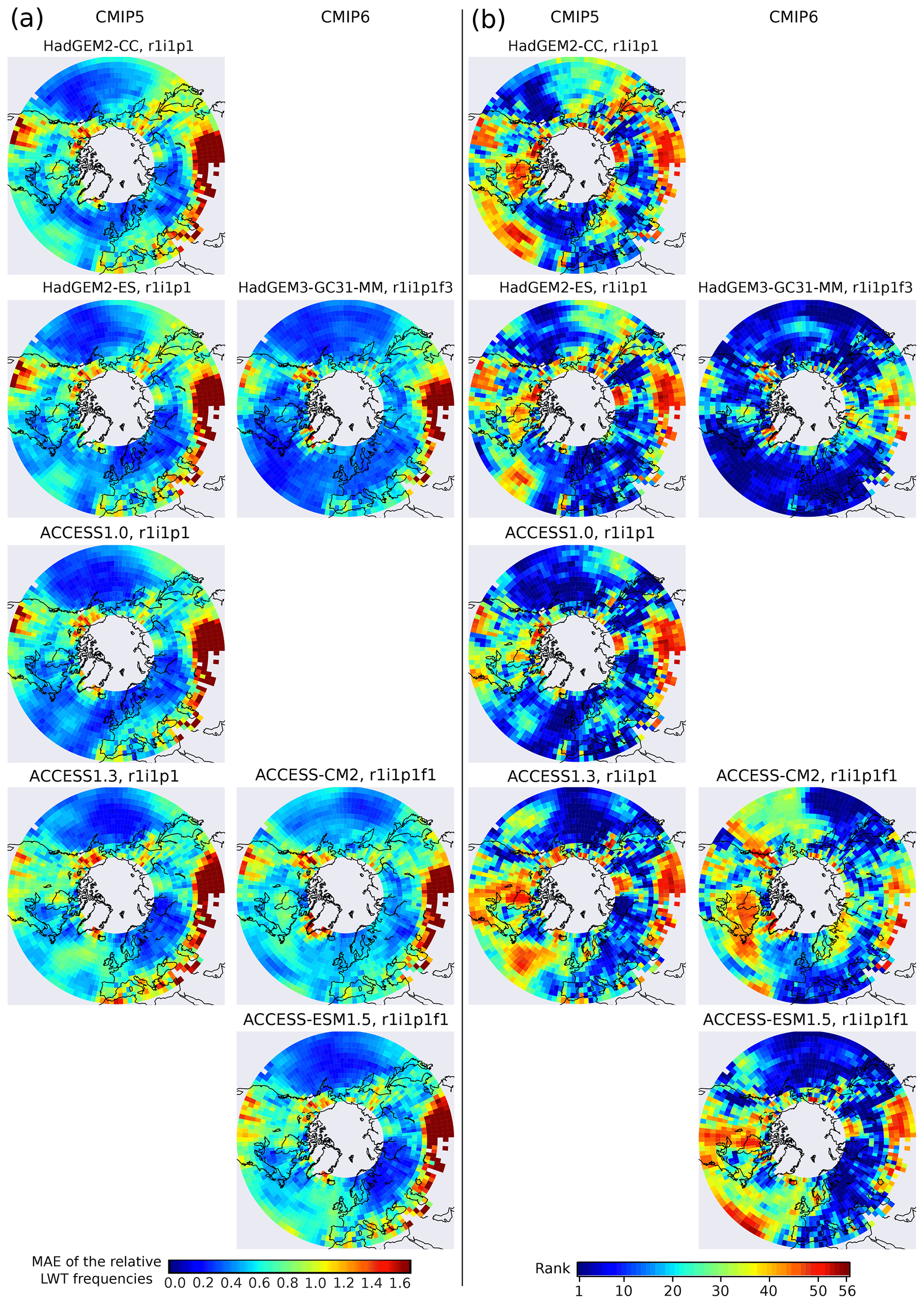
Figure 3Mean absolute error of the relative Lamb weather type frequencies from the historical CMIP experiments with respect to ERA-Interim (column a), as well as the respective rank within the 56 distinct model versions outlined in Table 1 (column b). The lower the rank, the lower the MAE and the better the model. Results are for the Met Office Hadley Centre and ACCESS model families. Model pairs from CMIP5 and 6 are plotted next to each other. Results are for the 1979–2005 period.
While CSIRO-MK was an independently developed GCM of the Australian research community (Collier et al., 2011), the Community Climate and Earth System Simulator (ACCESS) depends to a large degree on the aforementioned models from the Met Office Hadley Centre. ACCESS1.0, the starting point for the new Australian coupled model configurations, makes use of the same atmosphere and land-surface components as HadGEM2 (see above) but is run in a less complex configuration. It is considered the “control” configuration of all further developments made by the Australian modelling group (Bi et al., 2013). ACCESS1.3 is the first step into this direction. Instead of HadGAM2, it uses a slightly modified version of the Met Office Global Atmosphere 1.0 (GA1) AGCM, coupled with the CABLE1.8 land-surface model developed by CSIRO. ACCESS-CM2 is the AOGCM version used in CMIP6, relying on the UM10.6-GA7.1 AGCM (also used in HadGEM3-GC31-MM) and the CABLE2.5 coupler (Bi et al., 2020). ACCESS-CM2, however, was run with a lower horizontal resolution in the atmosphere than HadGEM3-GC31-MM. Whereas the three aforementioned ACCESS versions only have interactive aerosols on top of the four AOGCM components, ACCESS-ESM1.5 additionally includes interactive land and ocean carbon-cycle processes and prescribed vegetation properties. It uses slightly older AGCM and LSM versions (UM7.3-GA1 and CABLE2.4) than ACCESS-CM2 and makes use of the ocean biogeochemistry model WOMBAT (Ziehn et al., 2020). All ACCESS models use the same ocean and sea-ice models (GFDL-MOM and CICE), which differ from those used in the HadGEM model family. The OASIS coupler (Valcke, 2006) is applied by both model families.
Within the ACCESS model family, version 1.0 performs best (see Fig. 3). The corresponding error and ranking patterns are virtually identical to HadGEM2-ES and HadGEM2-CC, which is due to the same AGCM used in these three models (HadGAM2). The three more independent versions of ACCESS (1.3, CM2 and ESM1.5) roughly share the same error pattern, which differs from ACCESS1.0 in some regions. While they perform worse in the North Atlantic and western North Pacific, they do better in the eastern North Pacific off the coast of Japan and, in the case of ACCESS-CM2, also in the high-mountain areas of central Asia and over the Mediterranean Sea. In the latter two regions, the performance of ACCESS-CM2 is comparable to HadGEM3-GC31-MM. Overall, version 1.0 performs best within the ACCESS model family. For the sake of completeness, the performance maps for CSIRO-MK3.6 have been included in the Supplement.
The two HadGEM2 versions and ACCESS1.3 compare better with JRA-55 in the southwestern US but thrive towards ERA-Interim in the seas around Greenland and in the Gobi Desert. HadGEM3-GC31-MM, ACCESS1.0, ACCESS-CM2 and ACCESS-ESM1.5 have similar reanalysis affinities, except for thriving towards JRA-55 in the seas around Greenland and for showing virtually no sensitivity in the Gobi Desert in the case of ACCESS-ESM1.5 (compare Fig. 3 with the “figs-refjra55/maps/rank” folder in the Supplement).
4.2 Model contributions from North America
The Geophysical Fluid Dynamics Laboratory Climate Model 3 and 4 (GFDL-CM3 and CM4) are composed of in-house atmosphere, land-surface, ocean and sea-ice models and comprise interactive vegetation properties, aerosols and atmospheric chemistry (Griffies et al., 2011; Held et al., 2019). GFDL-CM4 also includes a simple ocean carbon-cycle representation which, however, does not feed back on other climate system components. From CM3 to CM4, a considerable resolution increase was undertaken, except for a reduction in the AGCM's vertical levels, and this actually pays off in terms of model performance (see Fig. 4). While GFDL-CM3 only ranks well in an area ranging from the Great Plains to the central North Pacific, GFDL-CM4 yields balanced results over the entire NH mid-to-high latitudes and is one of the best models considered here. Notably, GFDL-CM4 also performs well over central Asia and in an area ranging from the Black Sea to the Middle East, which is where most of the other models perform less favourable. Note also that GFDL's Modular Ocean Model (MOM) is the standard OGCM in all ACCESS models and is also used in the BCC-CSM model versions (see Table 1 for details).
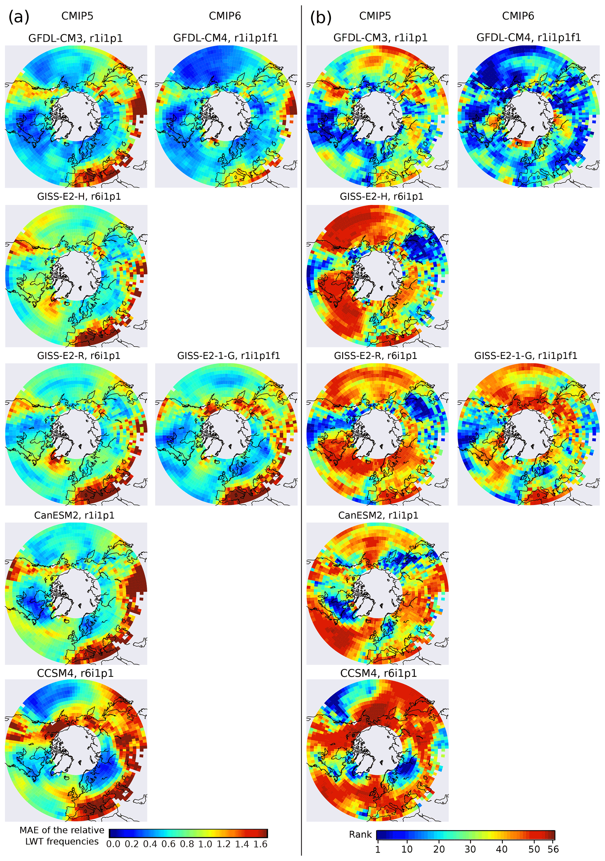
Figure 4As Fig. 3 but for the GFDL, GISS, CCCma and NCAR models.
All Goddard Institute of Space Studies model versions considered here are AOGCMs with prescribed vegetation properties, aerosols and atmospheric chemistry. The two versions are identical except for the ocean component: HYCOM was used in GISS-E2-H and Russel Ocean in GISS-E2-R (Schmidt et al., 2014). Russel Ocean was then developed to GISS Ocean v1 for use in GISS-E2.1-G (Kelley et al., 2020), the CMIP6 model version assessed here (note that the 6-hourly SLP data for the more complex model versions contributing to CMIP6 were not available from the ESGF data portals). All these versions comprise a relatively modest resolution for the atmosphere and ocean, and no refinement was undertaken from CMIP5 to 6. However, many parametrization schemes were improved. GISS-E2.1-G generally ranks better than its predecessors, except in eastern Siberia and China, where very good ranks are obtained by the two CMIP5 versions (see Fig. 4). The small differences between the results for GISS-E2-H and -R might stem from internal model variability (see also Sect. 4.9) and from the use of two distinct OGCMs. Unfortunately, all GISS-E2 model versions considered here are plagued by pronounced performance differences from one region to another, meaning that they are less balanced than, e.g. GFDL-CM4.
The National Center for Atmospheric Research (NCAR) Community Climate System Model 4 (CCSM4) is composed of the Community Atmosphere and Land Models (CAM and CLM), the Parallel Ocean Program (POP) and the Los Alamos Sea Ice Model (CICE), combined with the CPL7 coupler (Gent et al., 2011; Craig et al., 2012). The model version considered here was used in CMIP5 and includes interactive vegetation properties and land carbon-cycle processes, whereas aerosols are prescribed. During the course of the last decade, CCSM4 has been further developed into CESM1 and 2 (Hurrell et al., 2013; Danabasoglu et al., 2020) which, due to data availability issues, can unfortunately not be assessed here (the respective data for CESM2 are available but only for 15 out of the 27 considered years). However, CMCC-CM2 and NorESM2 are almost entirely made up by components from CESM1 and 2, respectively, and should thus be also indicative for the performance of the latter (see Sect. 4.8).
The Canadian Earth System Model version 2 (CanESM2) is composed of the CanAM4 AGCM, the CLASS2.7 land-surface model, the CanOM4 OGCM and the CanSIM1 sea-ice model (Chylek et al., 2011). It contributed to CMIP5 and comprises interactive vegetation properties, land and ocean carbon-cycle processes and aerosols, whilst the ice-sheet area is prescribed.
Results indicate a comparatively poor performance for both CCSM4 and CanESM2. Exceptions are found along the North American west coast and the Labrador Sea, where both models perform well; in the central to eastern subtropical Pacific and in northwestern Russia plus Finland, where CCSM4 performs well; and in Quebec, Scandinavia and eastern Siberian, where CanESM2 ranks well (see Fig. 4). As for the GISS models, both CCSM4 and CanESM2 are also plagued by large regional performance differences.
Regarding the models' reanalysis affinity, GFDL-CM3 thrives towards ERA-Interim in the seas around Greenland and towards JRA-55 in the Gobi Desert, while being almost insensitive to reanalysis choice in the southwestern US (compare Fig. 4 with the “figs-refjra55/maps/rank” folder in the Supplement). GFDL-CM4 has similar reanalysis affinities but largely improves (by up to 20 ranks) in the southwestern US when evaluated against JRA-55. Results for GISS-E2-H and GISS-E2-R are slightly closer to ERA-Interim in the southwestern US and otherwise virtually insensitive to reanalysis choice. GISS-E2-1-G is virtually insensitive in all three regions. CanESM2 ranks consistently better if compared with JRA-55, with a stunning improvement of up to 30 ranks in the southwestern United States, and CCSM4 slightly thrives towards ERA-Interim in all three regions.
4.3 Model contributions from France
The CMIP5 contributions from the Centre National de Recherches Météorologique (CNRM) and Institut Pierre-Simon Laplace (IPSL) use the same OGCM and coupler, i.e. the Nucleus for European Modelling of the Ocean (NEMO) model (Madec et al., 1998; Madec, 2008) and OASIS but differ in their remaining components. CNRM-CM5 comprises the ARPEGE AGCM, ISBA land-surface model and GELATO sea-ice model (Voldoire et al., 2013) whereas IPSL makes use of LMDZ, ORCHIDEE and LIM, respectively (Dufresne et al., 2013). For CNRM-CM6-1, these components were updated (Voldoire et al., 2019). All CNRM model versions considered here are AOGCMs with prescribed aerosols and atmospheric chemistry, except CNRM-ESM2-1 (Séférian et al., 2019), which additionally comprises interactive component models for vegetation properties, terrestrial carbon-cycle processes, aerosols, stratospheric chemistry and ocean biogeochemistry.
Within the CNRM model family, CNRM-CM5 is found to perform very well except in the central North Pacific, the southern US and in a subpolar belt extending from Baffinland in the west to western Russia in the east (see Fig. 5). This includes good performance over the Rocky Mountains and central Asia. From CNRM-CM5 to CNRM-CM6-1, performance gains are obtained in the central North Pacific, the southern US, Scandinavia and western Russia which, however, are compensated by performance losses in the entire eastern North Atlantic and in an area covering Manchuria, the Korean Peninsula and Japan. A similar picture is obtained for CNRM-ESM2-1, whereas a performance loss is observed for CNRM-CM6-1-HR. This is surprising since, in addition to improved parametrization schemes, the model resolution in the atmosphere and ocean was particularly increased in the latter model version.
All IPSL-CM model versions participating in CMIP5 and 6 comprise interactive vegetation properties and terrestrial carbon-cycle processes, as well as prescribed aerosols and atmospheric chemistry. Ocean biogeochemistry processes are simulated online but do not feed back on other components of the climate system. A simple representation of ice-sheet dynamics was included in IPSL-CM6A-LR (Boucher et al., 2020; Hourdin et al., 2020; Lurton et al., 2020) but is absent in IPSL-CM5A-LR and MR (Dufresne et al., 2013). The two model versions used in CMIP5 have been run with a modest horizontal resolution in the atmosphere (LMDZ) and ocean (NEMO). This changed for the better in IPSL-CM6A-LR, where a more competitive resolution was applied and all component models were improved. The result is a considerable performance increase from CMIP5 to CMIP6. Whereas both IPSL-CM5A-LR and IPSL-CM5A-MR perform poorly, IPSL-CM6A-LR does much better virtually anywhere in the NH mid-to-high latitudes, a finding that is insensitive to the effects of internal model variability (see Sect. 4.9).
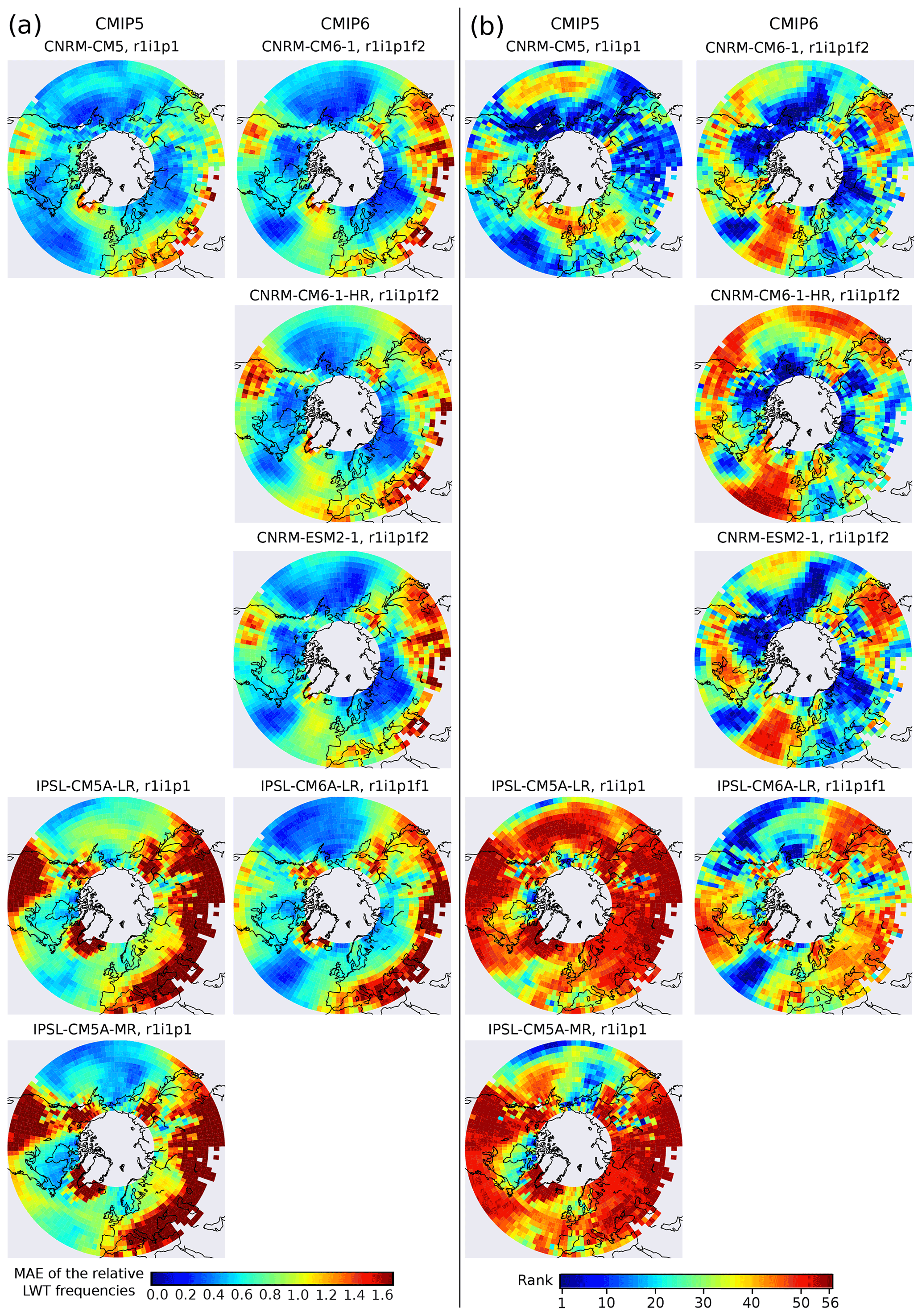
Figure 5As Fig. 3 but for the CNRM and IPSL models.
The quite different results between the CNRM and IPSL models indicate that the common ocean component (NEMO) only marginally affects the simulated atmospheric circulation as defined here. All CNRM models, and also IPSL-CM6A-LR, thrive towards ERA-Interim in the southwestern US and towards JRA-55 in the seas around Greenland and the Gobi Desert. IPSL-CM5A-LR and MR are virtually insensitive to reanalysis choice (compare Fig. 5 with the “figs-refjra55/maps/rank” folder in the Supplement).
4.4 Model contributions from China, Taiwan and India
The Beijing Climate Center Climate System Model version 1.1 (BCC-CSM1.1) comprises the BCC-AGCM2.1 AOGCM, originating from CAM3 and developed independently thereafter (Wu et al., 2008), the BCC-AVIM1.0 land-surface model developed by the Chinese Academy of Science (Jinjun, 1995), GFDL's MOM4-L40 ocean model and Sea Ice Simulator (SIS). For BCC-CSM2-MR, the coupled model version used in CMIP6 (Wu et al., 2019), the latest updates of the in-house models are used in conjunction with the CMIP5 versions of MOM and SIS (v4 and 2, respectively). Both BCC-CSM1.1 and BCC-CSM2-MR are composed of interactive vegetation properties, terrestrial and oceanic carbon-cycle processes, while aerosols and atmospheric chemistry are prescribed. The MAE and ranking patterns of the two models are quite similar to those obtained from NCAR's CCSM2 (compare Figs. 6 and 4), which is likely due to the common origin of their AGCMs, meaning that the two BCC-CSM versions are likewise found to perform comparatively poor in most regions of the NH mid-to-high latitudes. The similarity between both model families is astonishing since they only share the origin of their atmospheric component but rely on different land-surface, ocean and sea-ice models. This in turn means that the latter two components do not noticeably affect the simulated atmospheric circulation as defined here, which is in line with the large differences found for the French models in spite of using the same ocean model (see Sect. 4.3).
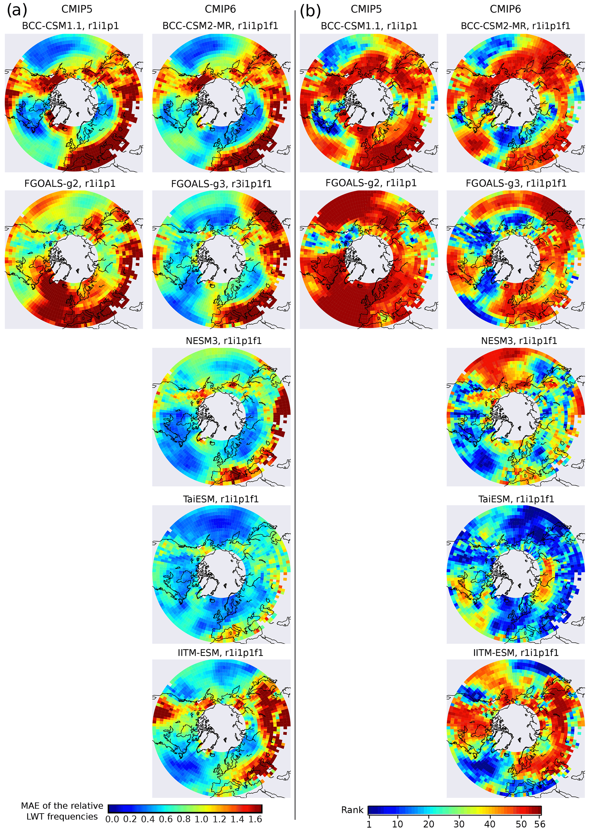
Figure 6As Fig. 3 but for the BCCR and FGOALS models, as well as for NESM3, TaiESM and IITM-ESM.
The Flexible Global Ocean-Atmosphere-Land System Model, Grid-point version 2 (FGOALS-g2) comprises an independently developed AGCM and OGCM (GAMIL2 and LICOM2), as well as CLM3 and CICE4-LASG for the land-surface and sea-ice dynamics, respectively (Li et al., 2013), all components being coupled with CPL6. Vegetation properties and aerosols are prescribed in this model configuration. For FGOALS-g3, the model version contributing to CMIP6, the AGCM was updated to GAMIL3, including convective momentum transport, stratocumulus clouds, anthropogenic aerosol effects and an improved boundary layer scheme as new features (Li et al., 2020). The OGCM and coupler were also updated (to LICOM3 and CPL7) and a modified version of CLM4.5 (called CAS-LSM) is used as a land-surface model, whereas the sea-ice model is practically identical to that used in the g2 version. In the g3 version, vegetation properties, terrestrial carbon-cycle processes and aerosols are prescribed. While FGOALS-g2 is one of the worst-performing models considered here, FGOALS-g3 performs considerably better, particularly over the northwestern and central North Atlantic Ocean, western North America and the North Pacific Ocean (see Fig. 6). The Nanjing University of Information Science and Technology Earth System Model version 3 (NESM3) is a new CMIP participant and is entirely built upon component models from other institutions (Cao et al., 2018). Namely, the AGCM, land-surface model, coupling software and atmospheric resolution are adopted from MPI-ESM1.2-LR (see Sect. 4.6) whereas NEMO3.4 and CICE4.1 are taken from IPSL and NCAR, respectively (Cao et al., 2018). Vegetation properties and terrestrial carbon-cycle processes are interactive, aerosols are prescribed. Due to the use of the same AGCM, the error and ranking patterns for NESM3 are similar to those obtained for MPI-ESM1.2-LR (compare Fig. 6 with Fig. 8). Exceptions are found over the central and western North Pacific, where NESM3 performs poorly compared to MPI-ESM1.2-LR, and also over the eastern North Pacific, where NESM3 performs better. The similarity to MPI-ESM1.2-LR again points to the fact that the simulated LWT frequencies are determined by the AGCM rather than other component models.
The Taiwan Earth System Model version 1 (TaiESM1) is run by the Research Center for Environmental Changes, Academia Sinica in Taipei. It is essentially identical to NCAR's Community Earth System Model version 1.2.2, including new physical and chemical parametrization schemes in its atmospheric component CAM5 (Lee et al., 2020). TaiESM1 comprises interactive vegetation properties, terrestrial carbon-cycle processes and aerosols. The model's performance is generally very good, except over northern Russia, northeastern North America and the adjacent northwestern Atlantic Ocean, and the error and ranking patterns are roughly similar to SAM0-UNICAN (see Fig. 6), another CESM1 derivative, with TaiESM1 performing much better over Europe.
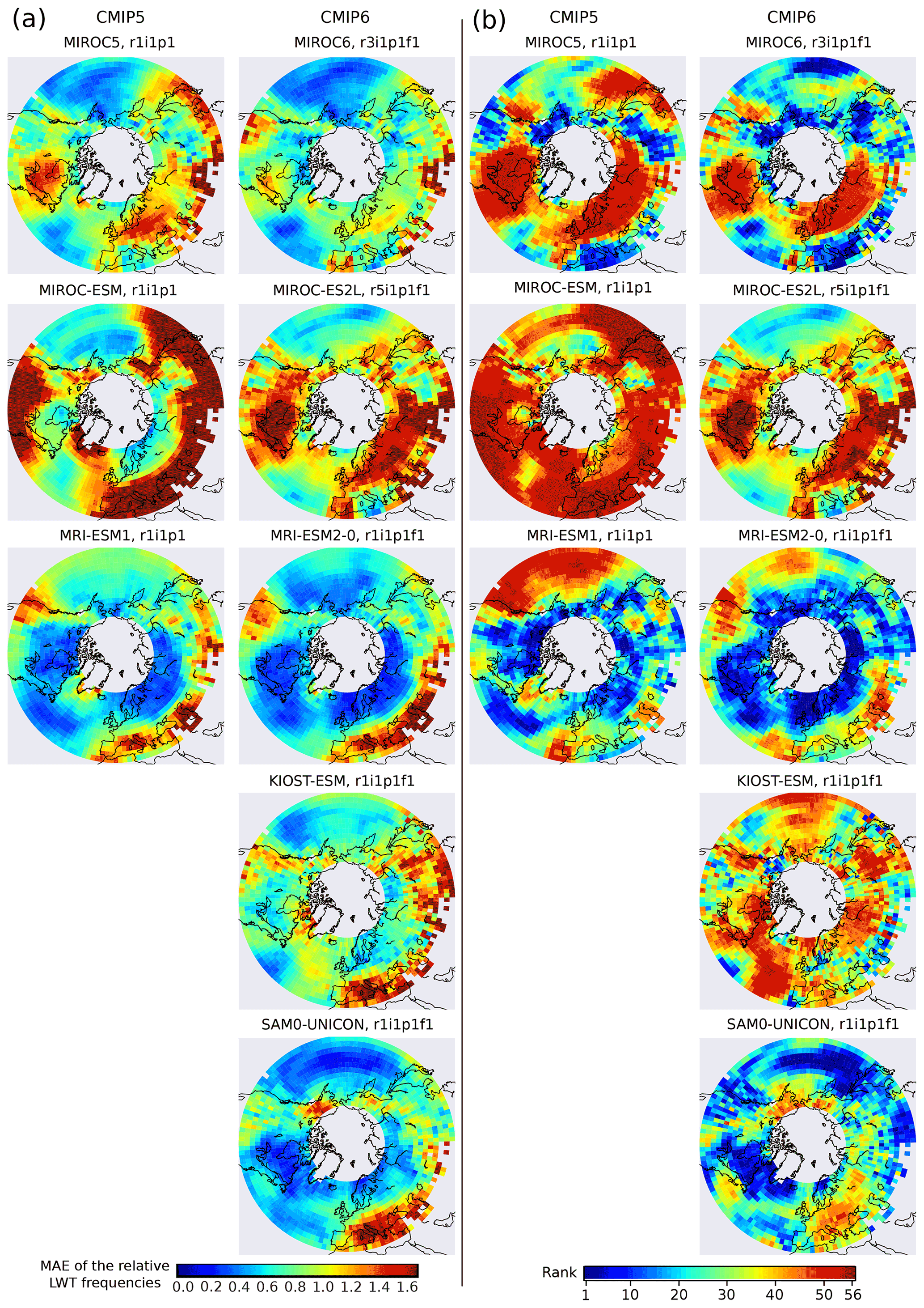
Figure 7As Fig. 3 but for the MIROC and MRI models, as well as KIOST-ESM and SAM0-UNICON.
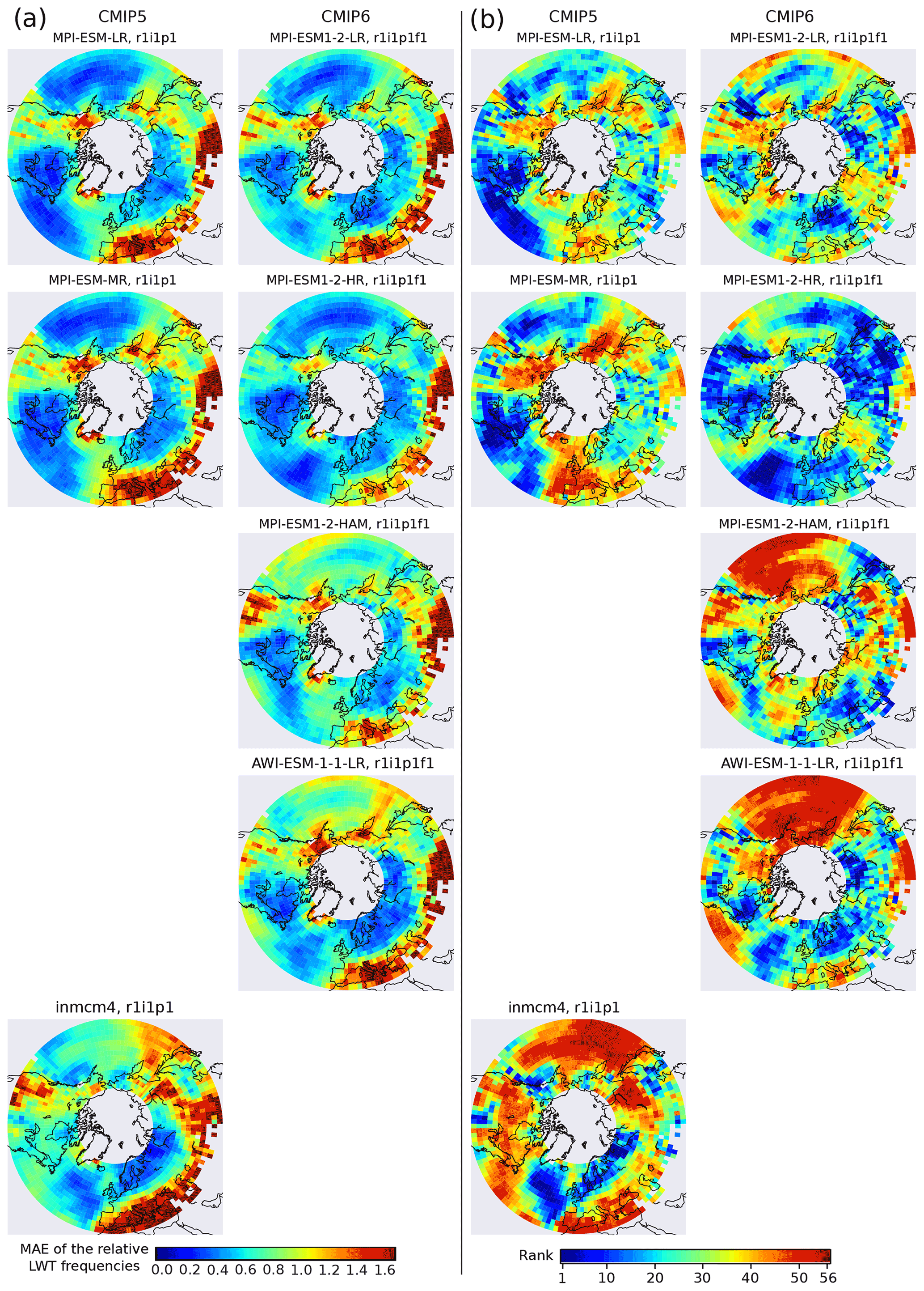
Figure 8As Fig. 3 but for the MPI, AWI and INM models.
The Indian Institute of Tropical Meteorology Earth System Model (IITM-ESM) includes the National Centers for Environmental Prediction Global Forecast System (NCEP GFS) AGCM, the MOM4p1 OGCM, Noah LSM for land-surface processes and SIS sea-ice dynamics (Swapna et al., 2015). Vegetation properties and aerosols are prescribed and ocean biogeochemistry processes are interactive. The results for IITM-ESM reveal large regional performance differences. The model ranks well over the central North Atlantic Ocean, Mediterranean Sea, the US west coast and subtropical western North Pacific but performs poorly in most of the remaining regions.
The results for BCC-CSM1.1, BCC-CSM2-MR and NESM3 are virtually insensitive to reanalysis uncertainty. To the southwest of Lake Baikal, both FGOALS-g2 and g3 are in closer agreement with JRA-55 than with ERA-Interim (compare Fig. 6 with the “figs-refjra55/maps/rank” folder in the Supplement). Over southwestern North America, however, FGOALS-g3 yields higher ranks if compared with ERA-Interim. TaiESM1 compares more closely with ERA-Interim over the southwestern US and the subtropical North Atlantic Ocean. The effects of reanalysis uncertainty on the results for IITM-ESM are generally small, except over the southern US, where JRA-55 yields better results, and in the seas surrounding Greenland, where the model agrees more closely with ERA-Interim.
4.5 Model contributions from Japan and South Korea
The Model for Interdisciplinary Research on Climate (MIROC) has been developed by the Japanese Center for Climate System Research (CCSR), National Institute for Environmental Studies (NIES) and the Japan Agency for Marine-Earth Science and Technology (JAMESTEC). It comprises the Frontier Research Center for Global Change (FRCGC) AGCM and CCSR's Ocean Component Model (COCO), as well as an own land-surface (MATSIRO) and sea-ice model. MIROC5 and 6 comprise interactive aerosols and prescribed vegetation properties (Watanabe et al., 2010; Tatebe et al., 2019). MIROC-ESM and MIROC-ESL2L are more complex configurations additionally including interactive terrestrial and ocean carbon-cycle processes, as well as interactive vegetation properties in the case of MIROC-ESM (Watanabe et al., 2011; Hajima et al., 2020). Results indicate a systematic performance increase from MIROC5 to MIROC6 in the presence of large performance differences from one region to another (see Fig. 6). Both models perform very well over the Mediterranean, northwestern North America and East Asia but do a poor job in northeastern North America and northern Eurasia. MIROC6 outperforms MIROC5 in the entire North Pacific basin including Japan, the Korean Peninsula and western North America and is also better in the central North Atlantic. The performance of the two more complex model versions is considerably lower, both ranking unfavourably if compared to the remaining GCM versions considered here.
The CMIP5 version of the Japanese Meteorological Research Institute Earth System Model (MRI-ESM1) comprises interactive component models for terrestrial carbon-cycle processes, aerosols, atmospheric photochemistry and ocean biogeochemistry, whereas vegetation properties are prescribed (Yukimoto et al., 2011). In the CMIP6 version (MRI-ESM2), terrestrial and ocean carbon-cycle processes are no longer interactive but prescribed from external files (Yukimoto et al., 2019). It is noteworthy that each model component and also the coupler have been originally developed by MRI, and the coupling applied in these models is particularly comprehensive (Yukimoto et al., 2011). The comparatively high model resolution applied in MRI-ESM1 was further refined in MRI-ESM2 by adding more vertical layers, particularly in the atmosphere (see Table 1). To the north of approximately 50∘ N, both model versions perform very well, except for Greenland and the surrounding seas in MRI-ESM1. Model performance decreases to the south of this line, particularly in the central to western Pacific basin including western North America, the subtropical North Atlantic to the west of the Strait of Gibraltar and the regions around Greenland and the Caspian Sea. It is in these “weak” regions where the largest performance gains are obtained from MRI-ESM1 to MRI-ESM2.
The Korea Institute of Ocean Science and Technology Earth System Model (KIOST-ESM) contains modified versions of GFDL-AM2.0 and CLM4 for atmosphere and land-surface dynamics, as well as GFDL-MOM5 and GFDL-SIS for ocean and sea-ice dynamics (Pak et al., 2021). The model has interactive representations for the vegetation properties and terrestrial carbon-cycle processes and works with prescribed aerosols. Its error and ranking patterns are similar to that obtained from GFDL-CM3 (using GFDL-AM3), the weakest performance found in the same regions (the western US, Mediterranean Basin, Manchuria and central North Pacific). However, KIOST-ESM consistently performs poorly compared to GFDL-CM3.
The Seoul National University Atmosphere Model version 0 with a Unified Convection Scheme (SAM0-UNICON) contributes for the first time in CMIP6 (Park et al., 2019). Its component models are identical to CESM1 in its AOGCM configuration plus interactive aerosols (Hurrell et al., 2013), including unique parametrization schemes for convection, stratiform clouds, aerosols, radiation, surface fluxes and planetary boundary layer dynamics (Park et al., 2019). Vegetation properties and terrestrial carbon-cycle processes are resolved interactively as well. Although the model components from CESM are used in SAM0-UNICON, CMCC-CM2-SR5 and NorESM2, a distinct error pattern is obtained for SAM0-UNICON (compare Fig. 7 with Fig. 10). This might be due to the use of different ocean models (see Table 1) or precisely due to the effects of the particular parametrization schemes mentioned above. Although the error magnitude of SAM0-UNICON is similar to CMCC-CM-SR5, SAM0-UNICON exhibits weaker regional performance differences, making it the more balanced model out of the two. In most regions of the NH mid-to-high latitudes, SAM0-UNICON yields better results than NorESM2-LM but is outperformed by NorESM2-MM.
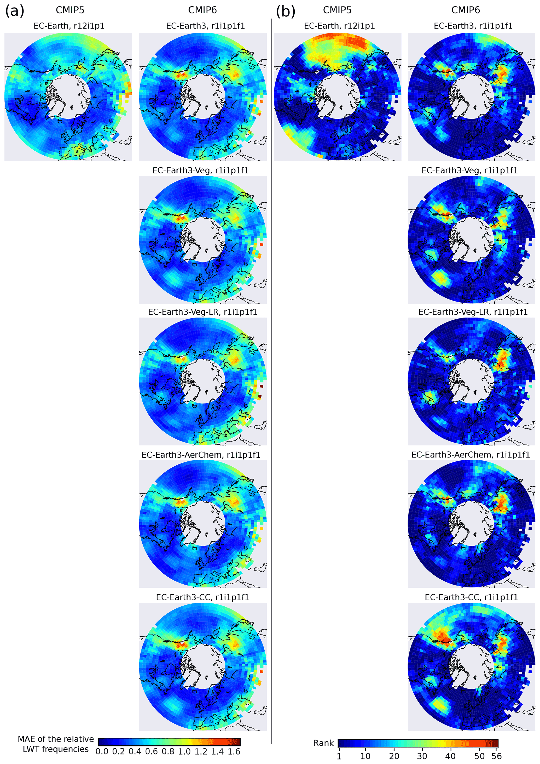
Figure 9As Fig. 3 but for the EC-Earth models.

Figure 10As Fig. 3 but for the CMCC and NorESM models.
The MRI models generally agree closer with ERA-Interim than with the JRA-55, which is surprising since JRA-55 was also developed at JMA (compare Fig. 7 with the “figs-refjra55/maps/rank” folder in the Supplement). For the MIROC family, a heterogeneous picture is obtained. While MIROC5 and MIROC-ESM clearly thrive towards ERA-Interim and JRA-55, respectively, MIROC6 is closer to JRA-55 in the southwestern US and closer to ERA-Interim in the Gobi Desert and around Greenland. The results for MIROC-ES2L are virtually insensitive to the applied reference reanalysis. In the three main regions of reanalysis uncertainty, SAM0-UNICON is in closer agreement with ERA-Interim than with JRA-55. For KIOST-ESM, it is the other way around. Over the southwestern US and Gobi Desert, this model more closely resembles JRA-55.
4.6 Model contributions from Germany and Russia
The Max-Planck Institute Earth System Model (MPI-ESM) is hosted by the Max-Planck Institute for Meteorology (MPI-M) in Germany, with all component models developed independently. It comprises the ECHAM, JSBACH, and MPIOM models representing atmosphere, land-surface and terrestrial biosphere processes as well as ocean and sea-ice dynamics (Giorgetta et al., 2013; Jungclaus et al., 2013; Mauritsen et al., 2019). All model configurations interactively resolve vegetation properties as well as terrestrial and ocean carbon-cycle processes, the latter represented by the HAMOCC model, and are coupled with the OASIS software. In MPI-ESM1.2-LR and -HR, aerosols are additionally prescribed. The “working horse” used for generating large ensembles and long control runs is the “LR” version applied in CMIP5 and 6 (MPI-ESM-LR and MPI-ESM1.2-LR, respectively). In this configuration, ECHAM (versions 6 and 6.3) is run with a horizontal resolution of 1.9∘ (T63) and 47 layers in the vertical, and MPIOM with a 1.5∘ resolution near the Equator and 40 levels in the vertical. In MPI-ESM-MR, the number of vertical layers in the atmosphere is doubled and the horizontal resolution in the ocean augmented to 0.4∘ near the Equator. In MPI-ESM1.2, several atmospheric parametrization schemes have been improved and/or corrected, including radiation, aerosols, clouds, convection and turbulence, and the land-surface and ocean biogeochemistry processes have been made more comprehensive. Since the carbon-cycle has not been run to equilibrium with MPI-ESM1.2-HR, this model version is considered unstable by its development team (Mauritsen et al., 2019). For MPI-ESM1.2-HAM, an aerosol and sulfur chemistry module, developed by a consortium led by the Leibniz Institute for Tropospheric Research, is coupled with ECHAM6.3 in a configuration that otherwise is identical to MPI-ESM1.2-LR (Tegen et al., 2019). Similarly, Alfred Wegener Institute's AWI-ESM-1.1-LR makes use of their own ocean and sea-ice model FESOM but otherwise is identical to MPI-ESM1.2-LR (Semmler et al., 2020).
Results show that the vertical resolution increase in the atmosphere undertaken from MPI-ESM-LR to MR (the CMIP5 versions) sharpens the regional performance differences rather than contributing to an improvement (see Fig. 8). When switching from MPI-ESM-LR to MPI-ESM1.2-LR, i.e. from CMIP5 to 6 with constant resolution, the performance increases over Europe but decreases in most of the remaining regions. Notably, MPI-ESM-LR's good to very good performance in a zonal belt ranging from the eastern subtropical North Pacific to the eastern subtropical Atlantic is lost in MPI-ESM1.2-LR. This picture worsens for MPI-ESM1.2-HAM and AWI-ESM-1.1-LR, which, even more so than MPI-ESM-MR, are characterized by large regional performance differences and particularly unfavourable results over almost the entire North Pacific basin. However, systematic performance gains are obtained by MPI-ESM1.2-HR, indicating that a horizontal rather than vertical resolution increase in the atmosphere conducts better performance in this model family (recall that the sole vertical resolution increase from MPI-ESM-LR to MPI-ESM-MR worsens the results). In the “HR” configuration, MPI-ESM1.2 is one of the best-performing models considered here.
The atmosphere, land-surface, ocean and sea-ice components of the Institute of Numerical Mathematics, Russian Academy of Sciences model INM-CM4 were all developed independently (Volodin et al., 2010). This model comprises interactive vegetation properties and terrestrial carbon-cycle processes, as well as a simple ocean carbon model, including atmosphere–ocean fluxes, total dissolved carbon advection by oceanic currents and a prescribed biological pump (Evgeny Volodin, personal communication). INM-CM4 contributed to CMIP5, and an updated version (INM-CM4-8) is currently participating in CMIP6, but the 6-hourly SLP data are not available for this version so it had to be excluded here. The resolution setup of INM-CM4 is comparable to other CMIP5 models, except for the very few vertical layers used in the atmosphere (see Table 1). As shown in Fig. 8, INM-CM4 performs well in the eastern North Atlantic, northern Europe and the Gulf of Alaska, regularly over northern China and the Korean Peninsula and poorly over the remaining regions of the NH. It is thus marked by large performance differences from one region to another.
In the three main regions sensitive to reanalysis uncertainty, all model versions assessed in this section consistently thrive towards JRA-55 (compare Fig. 8 with the “figs-refjra55/maps/rank” folder in the Supplement).
4.7 The joint European contribution EC-Earth
The EC-Earth consortium is a collaborative effort made by research institutions from several European countries. Following the idea of seamless prediction (Palmer et al., 2008), the atmospheric component used in the EC-Earth model is based on ECMWF's Integrated Forecasting System (IFS), complemented by the HTESSEL land-surface model and a new parametrization scheme for convection. NEMO and LIM constitute the ocean and sea-ice models; OASIS is the coupling software (Hazeleger et al., 2010, 2011). Starting from this basic AOGCM configuration, additional climate system components can be optionally added to augment the complexity of the model. Regarding the historical experiments for CMIP5 and 6, EC-Earth 2.3 (or simply EC-Earth) and 3 are classical AOGCM configurations, using prescribed vegetation properties and aerosols (in the case of EC-Earth3). EC-Earth3-Veg comprises interactive vegetation properties and terrestrial carbon-cycle processes, whereas aerosols are prescribed. EC-Earth3-AerChem incorporates the interactive aerosol model TM5 whilst vegetation properties are prescribed. EC-Earth3-CC contains interactive vegetation properties, terrestrial and ocean carbon-cycle processes. Aerosols are prescribed in this “carbon-cycle” model version. Already the model version used in CMIP5 (EC-Earth2.3) comprises a fine resolution in the atmosphere and ocean, except for the relatively few vertical layers in the ocean. This configuration was adopted and more ocean layers were added for what is named “low resolution” in CMIP6 (EC-Earth3-LR, EC-Earth3-Veg-LR). For the remaining configurations used in CMIP6 (EC-Earth3, EC-Earth3-Veg, EC-Earth3-AerChem, EC-Earth3-CC), the atmospheric resolution is further refined in the horizontal and vertical (Döscher et al., 2021).
Results reveal an already very good performance for EC-Earth2.3 in all regions except the North Pacific and subtropical central Atlantic (see Fig. 9), which is in line with Perez et al. (2014) and Otero et al. (2017). EC-Earth3 performs even better and does so irrespective of the applied model complexity or resolution. All the versions of this model rank very well in almost any region of the world, including the central Asian high-mountain areas.
When evaluated against JRA-55 instead of ERA-Interim, the ranks for the EC-Earth model family consistently worsen by up to 20 integers in the southwestern US and around the southern tip of Greenland but remain roughly constant in the Gobi Desert (compare Fig. 9 with the “figs-refjra55/maps/rank” folder in the Supplement). This worsening brings the EC-Earth family to a closer agreement with the HadGEM models. Consequently, when evaluated against JRA-55, HadGEM3-GC31-MM links up with EC-Earth3 in what is here found to be the “best model”.
4.8 Model contributions from Italy and Norway
The Centro Euro-Mediterraneo per i Cambiamenti Climatici (CMCC) models are mainly built upon component models from MPI, NCAR and IPSL. For CMCC-CM, ECHAM5 is used in conjunction with SILVA, a land-vegetation model developed in Italy (Fogli et al., 2009), and OPA8.2 (note that later OPA versions were integrated into the NEMO framework) plus LIM for ocean and sea-ice dynamics, respectively. The very high horizontal resolution in atmosphere (T159) is achieved at the expense of a low horizontal resolution in the ocean and comparatively few vertical layers in both realms, as well as by the fact that no further climate system components are considered by this model version (Scoccimarro et al., 2011). For the core model contributing to CMIP6 (CMCC-CM2), all of the aforementioned components except the OGCM were substituted by those available from CESM1 (Hurrell et al., 2013). For the model version considered here (CMCC-CM2-SR5), CAM5.3 is run in conjunction with CLM4.5. For ocean and sea-ice dynamics, NEMO3.6 (i.e. OPA's successor) and CICE are applied (Cherchi et al., 2019). The coupler changed from OASISv3 to CPLv7 (Valcke, 2006; Craig et al., 2012) and the interactive aerosol model MAM3 was included. CMCC-ESM2 is the most complex version in this model family, including the aforementioned aerosol model, activated terrestrial biogeochemistry in CLM4.5 and the use of BFM5.1 to simulate ocean biogeochemistry processes. Due to the completely distinct model setups, the error and ranking patterns substantially change from CMIP5 to 6 for this model family (see Fig. 10). While CMCC-CM performs relatively weak in northern Canada, Scandinavia and northwestern Russia, CMCC-CM2-SR5 does so in the North Atlantic, particularly to the west of the Strait of Gibraltar. In the remaining regions, very good ranks are obtained by both models. Notably, CMCC-CM2-SR5 is one of the few models performing well in the central Asian high-mountain ranges and also in the Rocky Mountains (except in Alaska). In most of the remaining regions, it is likewise one of the best models considered here. Note that this model, due to identical model components for all realms except the ocean, is a good estimator for the performance of CESM1, which unfortunately cannot be assessed here due to data availability issues. The error an ranking patterns of CMCC-ESM2 are similar to CMCC-CM2-SR5, yielding fewer regional differences and a much better performance over the central eastern North Atlantic Ocean. Hence, CMCC-ESM2 is not only the most sophisticated but also the best-performing model version in this family.
The Norwegian Earth System Model (NorESM) shares substantial parts of its source code with the NCAR model family (particularly with CCSM and CESM2). NorESM1-M, the standard model version used in CMIP5 (Bentsen et al., 2013), comprises the CAM4-Oslo AOGCM – derived from CAM4 and complemented with the Kirkevag et al. (2008) aerosol module – CLM4 for land-surface processes, CICE4 for sea-ice dynamics and an ocean model based on the Miami Isopycnic Coordinate Ocean Model (MICOM) originally developed by NASA/GISS (Bleck and Smith, 1990). CPL7 is used as coupler. NorESM1-M contains interactive terrestrial carbon-cycle processes and aerosols, whereas vegetation properties are prescribed. From NorESM1 to NorESM2, the model components from CCSM were updated to CESM2.1 (Danabasoglu et al., 2020) whilst keeping the Norwegian aerosol module and modifying a number of parametrization schemes in CAM6-Nor with respect to CAM6 (Seland et al., 2020). Through the coupling of an updated MICOM version with the ocean biogeochemistry model HAMOCC, combined with the use of CLM5, the terrestrial and ocean carbon-cycle processes are interactively resolved in NorESM2. Vegetation properties and atmospheric chemistry are prescribed, and the coupler has been updated from CPL7 to CIME, which is also used in CESM2. In the present study, the basic configuration NorESM2-LM is evaluated together with NorESM2-MM, the latter using a much finer horizontal resolution in the atmosphere (see Table 1). The corresponding maps in Fig. 10 reveal low model performance for NorESM1-M with an error magnitude and spatial pattern similar to CCSM4. When switching to NorESM2-LM, i.e. to updated and extended component models and an almost identical resolution in the atmosphere and ocean, notable performance gains are obtained in most regions of the NH, except in a zonal band extending from Newfoundland to the Ural Mountains which, further to the east, re-emerges over the Baikal region. In the higher-resolution version (NorESM2-MM), these errors are further reduced to a large degree, with the overall effect of obtaining one of the best models considered here.
In the three regions of pronounced reanalysis uncertainties, CMCC-CM is in closer agreement with JRA-55, whereas CMCC-CM2-SR5 and CMCC-ESM2 are more similar to ERA-Interim, reflecting the profound change in the model components from CMIP5 to 6 (compare Fig. 10 with the “figs-refjra55/maps/rank” folder in the Supplement). For the NorESM family, different reanalysis affinities are obtained for the three regions. While NorESM1 is closer to JRA-55 in all of them, NorESM2-LM is closer to ERA-Interim in the southwestern US but closer to JRA-55 in the Gobi Desert. NorESM2-MM is generally less sensitive to reanalysis uncertainty, with some affinity to ERA-Interim in the southwestern United States.
4.9 Summary boxplot, role of model resolution, model complexity and internal variability
For each model version listed in Table 1, the spatial distribution of the pointwise MAE values can also be represented with a boxplot instead of a map, which allows for an overarching performance comparison visible at a glance (see Fig. 11 for the evaluation against ERA-Interim). Here, the standard configuration of the boxplot is applied. For a given sample of MAE values corresponding to a specific model, the box refers to the interquartile range (IQR) of that sample and the horizontal bar to the median. Whiskers are drawn at the 75th percentile + 1.5 × IQR and at the 25th percentile − 1.5 × IQR. All values outside this range are considered outliers (indicated by dots). Four additional boxplots are provided for the joint MAE samples of the more complex model versions (reaching a score ≥ 14) and the less complex versions used in CMIP5 and 6. In these four cases, outliers are not plotted for the sake of simplicity. The abbreviations of the coupled model configurations, as well as their participation in either CMIP5 or 6 (indicated by the final integer), are shown below the x axis. Along the x axis, the names of the coupled models' atmospheric components are also shown since some of them are shared by various research institutions (see also Table 1).
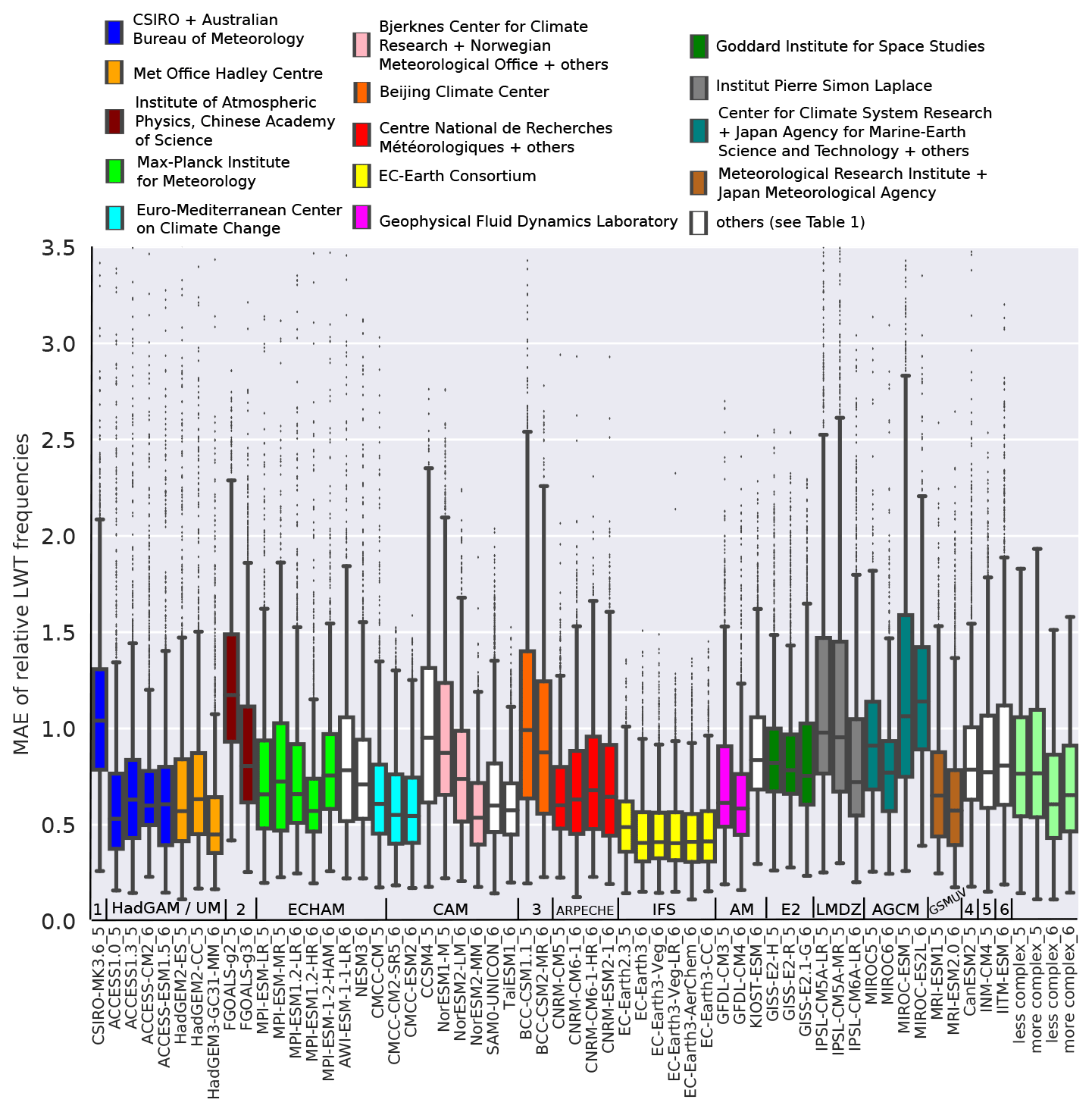
Figure 11Summary model performance plot; for each model version listed in Table 1, the pointwise MAE values are drawn with a boxplot instead of using a map. Four additional boxplots are provided for the less and the more complex model versions used in CMIP5 and 6, respectively (see text for details). Colours are assigned to the distinct coordinating research institutes, as indicated in the legend. The abbreviations of the coupled models, as well as their participation in either CMIP5 or 6 (indicated by the final integer) are shown below the x axis. Above this axis, the atmospheric component of each coupled model is shown in addition. Results are for the 1979–2005 period and with respect to ERA-Interim. AGCM abbreviations along the x axis are as defined as follows: (1) MK3 AGCM, (2) GAMIL, (3) BCC-AGCM, (4) CanAM4, (5) unnamed and (6) IITM-GFSv1; the names of the remaining AGCMs are indicated in the figure.
Results indicate a performance gain for most model families when switching from CMIP5 to 6 (available model pairs are located next to each other in Fig. 11). The largest improvements are obtained for those models performing relatively poorly in CMIP5. Namely, FGOALS-g2 improves upon FGOALS-g2 (dark brown), NorESM2-LM and NorESM2-MM upon NorESM1-M (rose), BCC-CSM1.1 upon BCC-CSM2-MR (orange), MIROC6 upon MIROC5 (blue-green) and IPSL-CM6A-LR upon IPSL-CM5A-LR and IPSL-CM5A-MR (grey). GISS-E2-R-5 improves upon GISS-E2-H and GISS-E2-R (green) in terms of median performance but suffers slightly larger spatial performance differences as indicated by the IQR. The MPI (neon green), CMCC (cyan), GFDL (magenta) and MRI (brown) models already performed well in CMIP5 and further improve in CMIP6. Among the MPI models, however, an advantage over the two CMIP5 versions is only obtained when considering the high-resolution CMIP6 version (compare MPI-ESM1.2-HR with MPI-ESM-LR and MPI-ESM-MR). Contrary to the remaining models, the performance of the CNRM (red) models does not improve from CMIP5 to 6, which may be due to the fact that the CMIP5 version (CNRM-CM5) already performed very well. Remarkably, CNRM's high-resolution CMIP6 version (CNRM-CM6-1-HR) is performing worst within this model family. Likewise, the ACCESS models (blue) do not improve either if ACCESS1.0 instead of ACCESS1.3 is taken as reference CMIP5 model.
The CMCC, HadGEM, and particularly the EC-Earth model families perform overly best, and all three exhibit a performance gain from CMIP5 to 6. NorESM2-MM also belongs to the best-performing models and largely improves upon NorESM2-LM and NorESM1. Remarkably, for four out of five possible comparisons, the more complex model version performs similar to less complex one (compare ACCESS-ESM1.5 with ACCESS-CM2, CMCC-ESM2 with CMCC-CM2-SR5, CNRM-ESM2-1 with CNRM-CM6-1-HR and EC-Earth3-CC with EC-Earth3). Only the MIROC family suffers a considerable performance loss when switching from less to more complexity, and only in this family the AGCM's resolution is considerably lower in the more complex configurations (compare MIROC-ESM with MIROC5 and MIROC-ES2L with MIROC6 in Fig. 11 and Table 1).
A virtual lack of outliers is another remarkable advantage of NorESM2-MM. MRI-ESM2 and GFDL-CM4 are also relatively robust to outliers but less so than NorESM2-MM. The fewest number of outliers among all models is obtained for EC-Earth, irrespective of the model version.
The model evaluation against JRA-55 reveals similar results (see “figs-refjra55/as-figure-10-but-wrt-jra55.pdf” in the Supplement), indicating that uncertain reanalysis data in the three relevant regions detected above do not substantially affect the hemispheric-wide statistics. What is noteworthy, however, is the slight but nevertheless visible performance loss for the EC-Earth model family, bringing EC-Earth3 approximately to the performance level of HadGEM3-GC31-MM. If evaluated against JRA-55, all EC-Earth model versions also comprise more outlier results. EC-Earth's affinity to ERA-Interim might be explained by the fact that this reanalysis was also built with ECMWF IFS.
Table 2 provides the rank correlation coefficients (rs) between the median MAE with respect to ERA-Interim for each model, corresponding to the horizontal bars within the boxes in Fig. 11, and various resolution parameters of the atmosphere and ocean component models. Correlations are calculated separately for the zonal, meridional and vertical resolution represented by the number of grid boxes in the corresponding direction. Due to the presence of reduced Gaussian grids, longitudinal grid boxes at the Equator are considered. In addition, the 2-D mesh defined as the number of longitudinal grid boxes multiplied by the number of latitudinal grid boxes, as well as the 3-D mesh defined as the number of longitudinal grid boxes multiplied by the number of latitudinal grid boxes multiplied by the number of vertical layers, is taken into account in the analysis. Correlations are first calculated separately for the atmosphere and ocean, and, in the last step, the sizes of the atmosphere and ocean 3-D meshes are added to obtain the size of the combined atmosphere–ocean mesh. All dimensions are obtained from the source attribute inside the NetCDF files from ESGF or directly from the data array stored therein. Note that due to an unstructured grid in one ocean model, the breakdown in zonal and meridional resolution cannot be made in this realm.
Table 2Rank correlation coefficients between the median MAE values of the 56 models and various resolution parameters of the atmosphere or/and ocean component models. A significant relationship is indicated by an asterisk (α=0.01, two-tailed t test, H0= zero correlation). See text for more details.
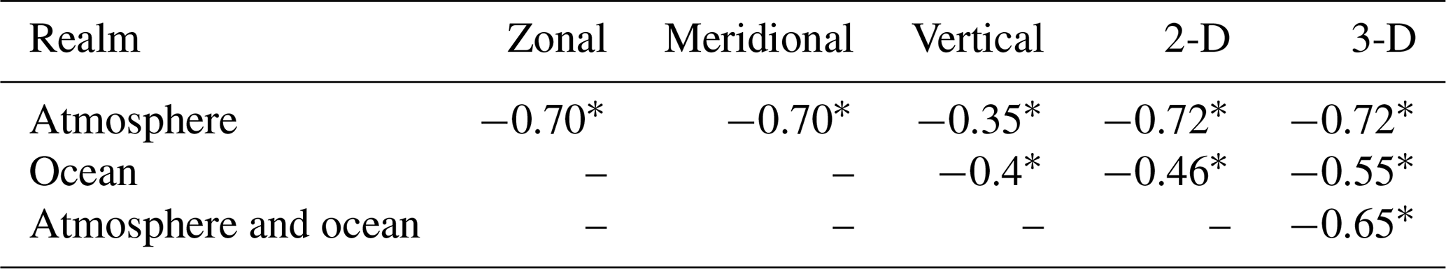
As can be seen from Table 2, average model performance is closer related to the horizontal than to the vertical resolution in the atmosphere. Associations with the ocean resolution are weaker, as expected, but nevertheless significant. Since the resolution increase for most models has gone hand in hand with improvements in the internal parameters (parametrization, model physics, bugs), it is difficult to say which of these two effects is more influential for model performance. However, most of the models undergoing a version change without resolution increase do not experience a clear performance gain either. This is observed for the three ACCESS versions using the same AGCM (i.e. GA in 1.3, CM2 and ESM1-5) and also for the three model versions from GISS, all comprising the same horizontal resolution in the atmosphere within their respective model family. Likewise, CNRM-CM6-1 and MPI-ESM1-2-LR even perform slightly worse than their predecessors (CNRM-CM5 and MPI-ESM-LR), meaning that the update is counterproductive for their performance (see Fig. 11). This points to the fact that resolution is likely more influential for performance than model updates as long as the latter are not too substantial. Interestingly, the relationship between the models' median performance and the horizontal mesh size of their atmospheric component is nonlinear (rs 0.72), with an abrupt shift towards better results at approximately 25 000 grid points (see Fig. 13a).

Figure 12As Fig. 11 but considering 72 additional runs for a subset of 13 distinct coupled models. All available runs per model are taken into account, except for IPSL-CM6A-LR for which the analyses were stopped after considering 17 additional ensemble members. The colours referring to the coordinating research institute are identical to those in Fig. 11, except for the Nanjing University of Information Science and Technology, which is painted white. Up to two ensembles per institute are shown, and the abbreviations of the individual coupled models are indicated by numbers. The exact run specifications are provided along the x axis.

Figure 13Relationship between the median performance of the coupled model configuration and (a) the horizontal mesh size of the atmospheric component or (b) the coupled model complexity score described in Sect. 3.3. Model performance is with respect to ERA-Interim. CNRM-CM6-1-HR and CNRM-ESM2-1 are out of scale in panel (a) due to their very fine atmospheric resolution.
Figure 13b shows the complexity score described in Sect. 3.3, plotted against the coupled models' median performance. The figure reveals that the best-performing model family (EC-Earth) is not the most complex one, and that some model configurations performing less well are particularly complex (e.g. CNRM-ESM2-1). Also, performance is generally unrelated to complexity, which is an argument in favour of including more component models to reach a more complete representation of the climate system. Interestingly, for four out of five possible comparisons, the most complex model configuration within a given family performs similar to the less complex ones if the AGCM's horizontal resolution is not reduced (compare ACCESS-ESM1.5 with ACCESS-CM2, CMCC-ESM2 with the CMCC-CM2-SR5, CNRM-ESM2-1 with CNRM-CM6-1-HR and CNRM-CM6-1-HR and EC-Earth3-CC with EC-Earth3). Within the MIROC family, this resolution was reduced in the more complex configurations and a systematic performance decrease is observed (compare MIROC5 with and MIROC6 with MIROC-ES2L).
In comparison with the inter-model variability discussed above, the internal model variability (or “intra-model variability”) is much smaller and only marginally affects the results, which for all runs of a given model version are in close agreement even for the outliers (see Fig. 12). Although the use of alternative model runs might lead to slight shifts in the ranking order at the grid-box scale, a “good” rank would not change into an “average” or even “bad” one. However, while internal model variability only plays a minor role in the context of the present study, some specific models indeed seem to be more sensitive to initial conditions uncertainty (which is where ensemble spread stems from in the experiments considered here) than others, with NorESM2-LM (the lower-resolution version only) and NESM3 seemingly being less stable in this sense. Remarkably, MPI-ESM1.2-HR is found to be stable in spite of the fact that it is considered a more “unstable” configuration by its development team because the carbon-cycle had not been run to equilibrium for this version (Mauritsen et al., 2019). It is also good news that HadGEM2-ES, known to perform well for r1i1p1 and consequently used as baseline for many downscaling applications and impact studies of the past (Gutiérrez et al., 2013; Perez et al., 2014; San-Martín et al., 2016), performs nearly identical for r2i1p1. Lastly, the large performance increase from IPSL-CM5A-LR to IPSL-CM6A-LR is likewise robust to the effects of internal variability.
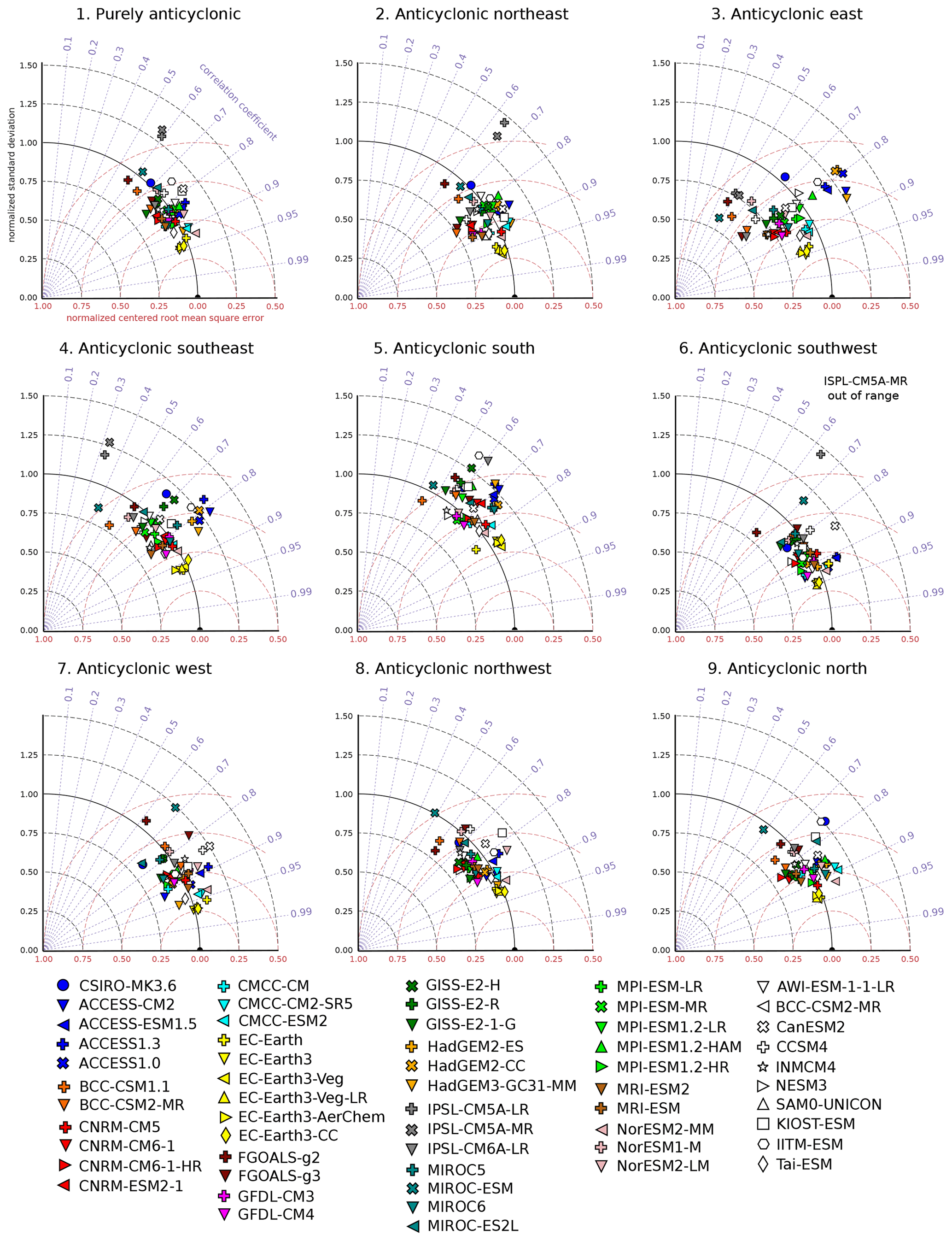
Figure 14Normalized Taylor diagram for the simulated vs. quasi-observed (from ERA-Interim) relative frequency pattern of a given Lamb weather type between 35∘–70∘ N. Each panel corresponds to a specific LWT, and each of the 56 considered models can be identified by a specific marker and colour, as indicated in the legend. Models pertaining to the same coordinating institution have the same colour. Shown are the results for the nine anticyclonic Lamb weather types.
In Figs. 14 to 16, the simulated, hemispheric-wide frequency pattern for a given model and LWT is compared with the respective quasi-observed frequency pattern obtained from ERA-Interim by using a normalized Taylor diagram (Taylor, 2001). The first thing to note here is that, for most LWTs, the models tend to cluster in a region that would be generally considered a good result. Except for some outlier models and individual LWTs, the pattern correlation lies in between 0.6 and 0.9, the standard deviation ratio is not too far from unity (equal to the best result) and the centred normalized RMSE ranges between 0.25 and 0.75 times the standard deviation of the observed frequency pattern.
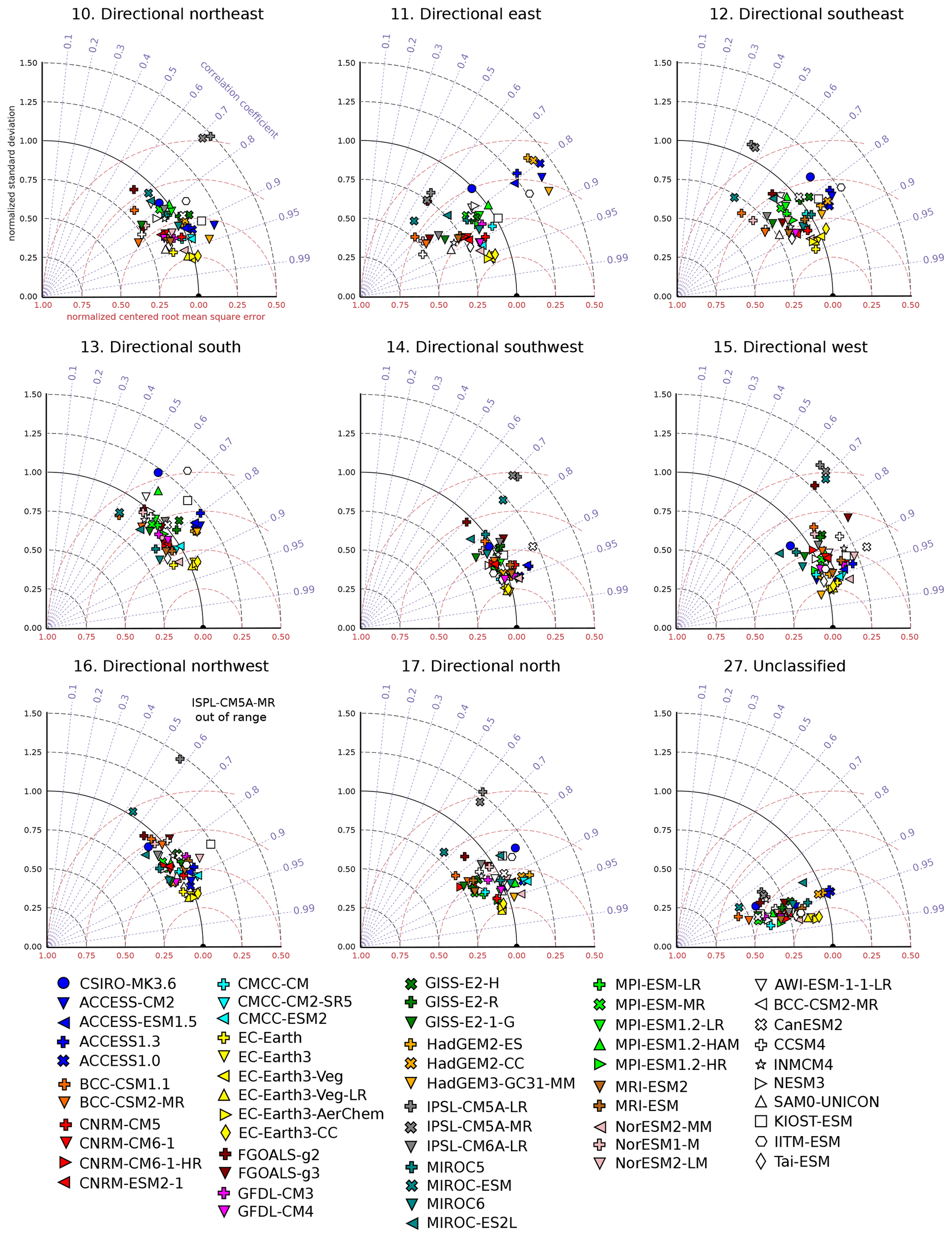
Figure 15As Fig. 14 but for the eight purely directional Lamb weather types and the unclassified type.
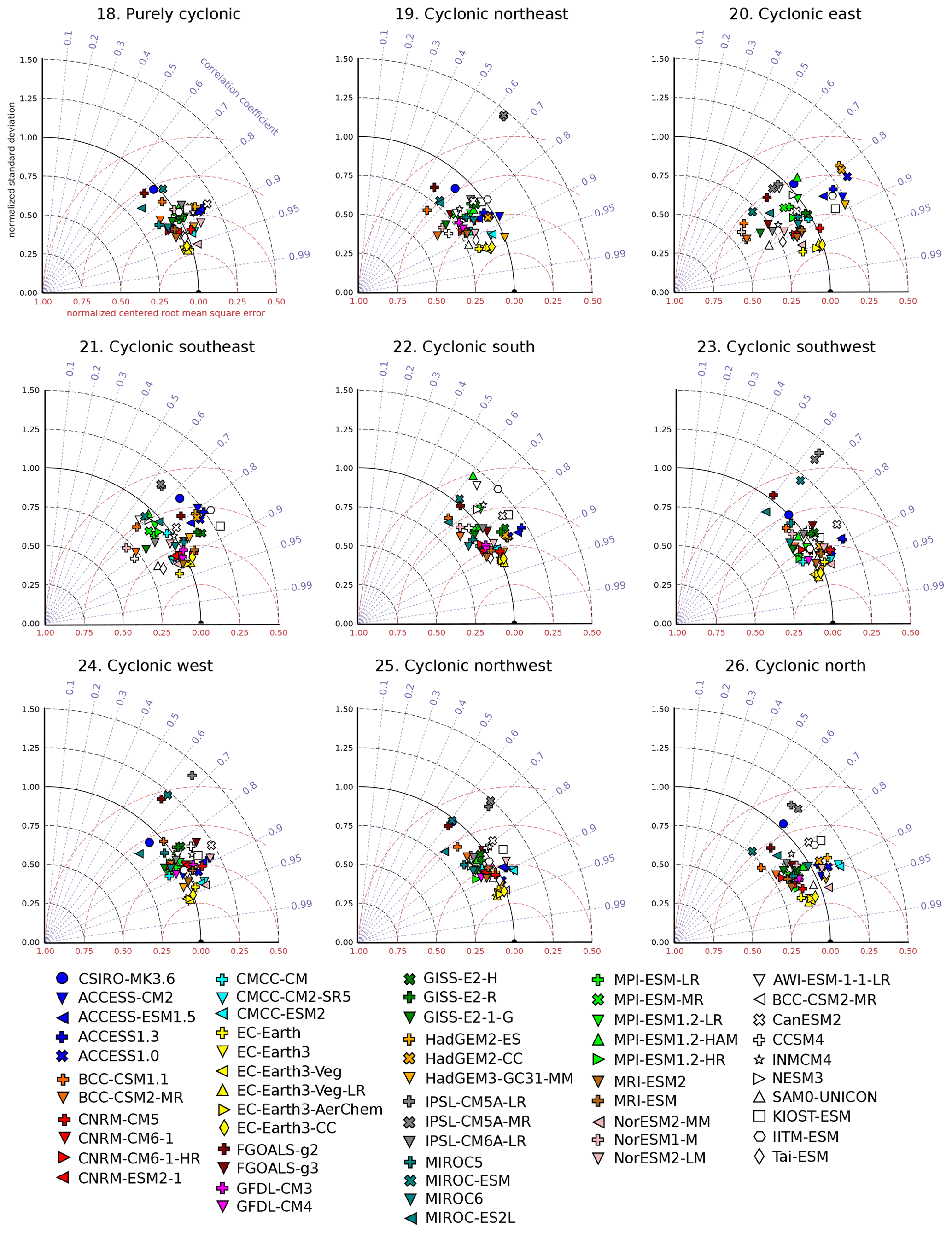
It is also found that all members of the EC-Earth model family yield best results for any LWT (observe the proximity of the yellow cluster to the perfect score indicated by the black half circle). Within the group of the more complex models, NorESM2-MM (the rose triangle pointing to the left) performs best and actually lies in close proximity to the EC-Earth cluster for most LWTs. The Hadley Centre and ACCESS models (filled with orange and dark blue) form another cluster that generally perform very well for most LWTs. However, the spatial standard deviation of the three eastern LWTs (cyclonic, anticyclonic and directional) is overestimated by these models, which is indicated by a standard deviation ratio of ≈ 1.25, while values close to unity or below are obtained for the remaining models. It is also worth mentioning that not only ACCESS1.0 but also the other, more independently developed ACCESS versions pertain to this cluster, which indicates the common origin of their atmospheric component (the Met Office Hadley Centre) even at the level of detail of specific weather types. For all other models, the LWT-specific results do not largely deviate from the overall MAE results shown in Sect. 4, meaning that overall performance is generally also a good indicator of LWT-specific performance. As an example, MIROC-ESM (the blue-green cross), IPSL-CM5A-LR and IPSL-CM5A-LR (the grey cross and grey plus) are located in the “weak” area of the Taylor diagram for each of the 27 LWTs, which is in line with the likewise weak overall performance obtained for these models in Sect. 4.
The corresponding results for the model evaluation against JRA-55 are generally in close agreement with those mentioned above, except for the EC-Earth model family performing slightly less favourably (see “figs-refjra55/taylor” folder in the Supplement to this article).
In the present study, 56 coupled general circulation model versions contributing historical experiments to CMIP5 and 6 have been evaluated in terms of their capability to reproduce the observed frequency of the 27 atmospheric circulation types originally proposed by Lamb (1972), as represented by the ERA-Interim or JRA-55 reanalyses. The outcome is an objective, regional-scale ranking catalogue that is expected to be of interest for the model development teams themselves and also for the downscaling and regional climate model community asking for model selection criteria. In this context, the present study is a direct response to the claim for a circulation-based model performance assessment made by Maraun et al. (2017). In addition, a straightforward method to describe the complexity of the coupled model configurations in terms of considered climate system components has been proposed.
On average, the model versions used in CMIP6 perform better than their CMIP5 predecessors. This finding is in line with Cannon (2020) and Fernandez-Granja et al. (2021), and it holds for the more and the less complex model configurations as defined here. Among a number of tested resolution parameters, the horizontal resolution in the atmosphere is closest related to performance, with equal contributions from the latitudinal and longitudinal resolution and a weaker relationship with the number of vertical layers. An abrupt shift towards better model results at a horizontal mesh size of approximately 25 000 grid points is observed (see Fig. 13a), which might point to the existence of a minimum atmospheric resolution that should be maintained while augmenting the complexity of the coupled model configurations. The corresponding links with the ocean resolution are weaker but nevertheless significant.
Improving the internal model parameters (physics and parametrization schemes) and/or adding more vertical layers to the atmosphere seems to have little effect on model performance if the horizontal resolution is not refined in addition. This is the case for ACCESS-CM2 with respect to ACCESS1.3, CNRM-CM6-1 with respect to CNRM-CM5, GISS-E2-1-G with respect to GISS-ES-R and MPI-ESM1.2-LR with respect to MPI-ESM-LR.
For a subgroup of 13 out of 56 models, the impact of internal model variability on the performance was assessed with 72 additional historical model integrations, each one initialized from a unique starting date of the corresponding pre-industrial control run. The thereby-created initial conditions' uncertainty has little effect on the overall results. Although the point-wise ranking order might change by a few integers when alternative runs are evaluated, which is why a “best model” map is intentionally not provided here, a well-performing model would not even change to an “intermediate” one, or vice versa if another ensemble member was put to the test. A similarly small effect was found for changing the reference reanalysis from ERA-Interim to JRA-55, except in the following three problematic regions, where reanalysis uncertainties can substantially affect the models' ranking order: the southwestern United States, the Gobi Desert, and Greenland plus the surrounding seas.
Since the inclusion of more component models in a coupled model configuration provides a more realistic representation of the climate system and also yields distinguishable future scenarios (Séférian et al., 2019; Jones, 2020), it would make sense to consider this as an additional model selection criterion in future studies. The approach proposed here is intended to be a straightforward starting point to measure this criterion. It should be further refined as soon as more detailed model documentation, already provided for some climate system components (Séférian et al., 2020), becomes available in a systematic way, e.g. via the Earth System Documentation project (https://es-doc.org/, last access: 11 February 2022).
Complementary to Brunner et al. (2020), the here-provided metadata about the participating component models can also be used to estimate the a priori degree of dependence between the numerous coupled model configurations used in CMIP.
The ocean grids referred to in Table 1 are defined as follows: ORCA2 = 182×149, 2∘ with meridional refinement to 0.5∘ near the Equator; ORCA1 = 362×292, 1∘ with meridional refinement to near the Equator; ORCA05 = 722×511, 0.5∘ with no refinement; ORCA025 = 1442×1050, 0.25∘ with no refinement; eORCA1.3 = 362×332, 1∘ with meridional refinement to near the Equator; eORCA1 = 360×330, 1∘ with meridional refinement to near the Equator; eORCA025 = 1440×1205, 0.25∘ with no refinement.
The NetCDF files containing the Lamb weather type catalogues computed for this study have been permanently archived at https://doi.org/10.5281/zenodo.4452080 (Brands, 2021). The underlying Python code and particularly the function get_historical_metadata.py, containing extensive metadata about the coupled model configurations and their individual components, was stored at https://doi.org/10.5281/zenodo.4555367 (Brands, 2021).
The supplement related to this article is available online at: https://doi.org/10.5194/gmd-15-1375-2022-supplement.
The contact author has declared that there are no competing interests.
Publisher's note: Copernicus Publications remains neutral with regard to jurisdictional claims in published maps and institutional affiliations.
I am grateful to Jesús Fernández (CSIC, Spain) and Joaquín Bedia (UC, Spain) for discussing the manuscript and would like to thank the following model developers for revising the complexity codes provided in Table 1: Jian Cao (NUIST, China), Bin Wang (IPRC, Hawaii), Laurent Li (LMD, France), Tongwen Wu (Beijing Climate Center, China), Evgeny Volodin (INM, Russia), Hiroaki Tatebe (JAMSTEC, Japan), Swapna Panickal (IITM, India), YoungHo Kim (Pukyong National University, South Korea), Thorsten Mauritsen (MPI, Germany), Øyvind Seland (Norwegian Meteorological Institute), Seiji Yukimoto (MRI, Japan), Klaus Wyser and Ralf Döscher (SMHI, Sweden), Annalisa Cherchie and Enrico Scoccimarro (CMCC, Italy), Aurore Voldoire and Roland Séférian (CNRM, France), Olivier Boucher (IPSL, France), Peter Gent (NCAR, USA), Tido Semmler (AWI, Germany), Gill Martin (Met Office, UK), Huan Guo (GFDL/NOAA, USA) and Ina Tegen (TROPOS, Germany). I would also like thank the Agencia para la Modernización Tecnológica de Galicia (AMTEGA) and the Centro de Supercomputación de Galicia (CESGA) for providing the necessary computational resources.
This paper was edited by Juan Antonio Añel and reviewed by Andreas Dobler and two anonymous referees.
AMS: General Circulation Model, Glossary of Meteorology, https://glossary.ametsoc.org/wiki/General_circulation_model (last access: 11 February 2022), 2020. a
Bentsen, M., Bethke, I., Debernard, J. B., Iversen, T., Kirkevåg, A., Seland, Ø., Drange, H., Roelandt, C., Seierstad, I. A., Hoose, C., and Kristjánsson, J. E.: The Norwegian Earth System Model, NorESM1-M – Part 1: Description and basic evaluation of the physical climate, Geosci. Model Dev., 6, 687–720, https://doi.org/10.5194/gmd-6-687-2013, 2013. a, b
Bi, D., Dix, M., Marsland, S. J., O'Farrell, S., Rashid, H., Uotila, P., Hirst, A., Kowalczyk, E., Golebiewski, M., Sullivan, A., Yan, H., Hannah, N., Franklin, C., Sun, Z., Vohralik, P., Watterson, I., Zhou, X., Fiedler, R., Collier, M., Ma, Y., Noonan, J., Stevens, L., Uhe, P., Zhu, H., Griffies, S., Hill, R., Harris, C., and Puri, K.: The ACCESS coupled model: description, control climate and evaluation, Aust. Meteorol. Ocean. J., 63, 41–64, https://doi.org/10.22499/2.6301.004, 2013. a, b, c
Bi, D., Dix, M., Marsland, S., O’Farrell, S., Sullivan, A., Bodman, R., Law, R., Harman, I., Srbinovsky, J., Rashid, H., Dobrohotoff, P., Mackallah, C., Yan, H., Hirst, A., Savita, A., Dias, F. B., Woodhouse, M., Fiedler, R., and Heerdegen, A.: Configuration and spin-up of ACCESS-CM2, the new generation Australian Community Climate and Earth System Simulator Coupled Model, Journal of Southern Hemisphere Earth Systems Science, 70, 225–251, https://doi.org/10.1071/ES19040, 2020. a, b
Bleck, R. and Smith, L. T.: A wind-driven isopycnic coordinate model of the north and equatorial Atlantic Ocean: 1. Model development and supporting experiments, J. Geophys. Res.-Oceans, 95, 3273–3285, https://doi.org/10.1029/JC095iC03p03273, 1990. a
Boucher, O., Servonnat, J., Albright, A. L., Aumont, O., Balkanski, Y., Bastrikov, V., Bekki, S., Bonnet, R., Bony, S., Bopp, L., Braconnot, P., Brockmann, P., Cadule, P., Caubel, A., Cheruy, F., Codron, F., Cozic, A., Cugnet, D., D'Andrea, F., Davini, P., de Lavergne, C., Denvil, S., Deshayes, J., Devilliers, M., Ducharne, A., Dufresne, J.-L., Dupont, E., Éthé, C., Fairhead, L., Falletti, L., Flavoni, S., Foujols, M.-A., Gardoll, S., Gastineau, G., Ghattas, J., Grandpeix, J.-Y., Guenet, B., Guez, Lionel, E., Guilyardi, E., Guimberteau, M., Hauglustaine, D., Hourdin, F., Idelkadi, A., Joussaume, S., Kageyama, M., Khodri, M., Krinner, G., Lebas, N., Levavasseur, G., Lévy, C., Li, L., Lott, F., Lurton, T., Luyssaert, S., Madec, G., Madeleine, J.-B., Maignan, F., Marchand, M., Marti, O., Mellul, L., Meurdesoif, Y., Mignot, J., Musat, I., Ottlé, C., Peylin, P., Planton, Y., Polcher, J., Rio, C., Rochetin, N., Rousset, C., Sepulchre, P., Sima, A., Swingedouw, D., Thiéblemont, R., Traore, A. K., Vancoppenolle, M., Vial, J., Vialard, J., Viovy, N., and Vuichard, N.: Presentation and Evaluation of the IPSL-CM6A-LR Climate Model, J. Adv. Model. Earth Sy., 12, e2019MS002010, https://doi.org/10.1029/2019MS002010, 2020. a, b
Brands, S.: Which ENSO teleconnections are robust to internal atmospheric variability?, Geophys. Res. Lett., 44, 1483–1493, https://doi.org/10.1002/2016GL071529, 2017. a
Brands, S.: A circulation-based performance atlas of the CMIP5 and 6 models for regional climate studies in the northern hemisphere, Zenodo [data set], https://doi.org/10.5281/zenodo.4452080, 2021. a, b
Brands, S.: Python code to calculate Lamb circulation types for the northern hemisphere derived from historical CMIP simulations and reanalysis data, Zenodo [code], https://doi.org/10.5281/zenodo.4555367, 2022. a, b
Brands, S., Gutiérrez, J. M., Herrera, S., and Cofiño, A. S.: On the Use of Reanalysis Data for Downscaling, J. Climate, 25, 2517–2526, https://doi.org/10.1175/JCLI-D-11-00251.1, 2012. a
Brands, S., Herrera García, S., Fernández, J., and Gutiérrez, J.: How well do CMIP5 Earth System Models simulate present climate conditions in Europe and Africa? A performance comparison for the downscaling community, Clim. Dynam., 41, 803–817, https://doi.org/10.1007/s00382-013-1742-8, 2013. a, b
Brands, S., Herrera, S., and Gutiérrez, J.: Is Eurasian snow cover in October a reliable statistical predictor for the wintertime climate on the Iberian Peninsula?, Int. J. Climatol., 34, 1615–1627, https://doi.org/10.1002/joc.3788, 2014. a, b
Brunner, L., Pendergrass, A. G., Lehner, F., Merrifield, A. L., Lorenz, R., and Knutti, R.: Reduced global warming from CMIP6 projections when weighting models by performance and independence, Earth Syst. Dynam., 11, 995–1012, https://doi.org/10.5194/esd-11-995-2020, 2020. a
Cannon, A.: Reductions in daily continental-scale atmospheric circulation biases between generations of Global Climate Models: CMIP5 to CMIP6, Environ. Res. Lett., 15, 064006, https://doi.org/10.1088/1748-9326/ab7e4f, 2020. a
Cao, J., Wang, B., Yang, Y.-M., Ma, L., Li, J., Sun, B., Bao, Y., He, J., Zhou, X., and Wu, L.: The NUIST Earth System Model (NESM) version 3: description and preliminary evaluation, Geosci. Model Dev., 11, 2975–2993, https://doi.org/10.5194/gmd-11-2975-2018, 2018. a, b, c
Cherchi, A., Fogli, P. G., Lovato, T., Peano, D., Iovino, D., Gualdi, S., Masina, S., Scoccimarro, E., Materia, S., Bellucci, A., and Navarra, A.: Global Mean Climate and Main Patterns of Variability in the CMCC-CM2 Coupled Model, J. Adv. Model. Earth Sy., 11, 185–209, https://doi.org/10.1029/2018MS001369, 2019. a, b, c
Chylek, P., Li, J., Dubey, M. K., Wang, M., and Lesins, G.: Observed and model simulated 20th century Arctic temperature variability: Canadian Earth System Model CanESM2, Atmos. Chem. Phys. Discuss., 11, 22893–22907, https://doi.org/10.5194/acpd-11-22893-2011, 2011. a, b
Collier, M., Jeffrey, S., Rotstayn, L., Wong, K.-H., Dravitzki, S., Moeseneder, C., Hamalainen, C., Syktus, J., Suppiah, R., Antony, J., El Zein, A., and Atif, M.: The CSIRO-Mk3.6.0 Atmosphere Ocean GCM: participation in CMIP5 and data publication, 19th International Congress on Modelling and Simulation. Modelling and Simulation Society of Australia and New Zealand, 2691–2697, Perth, Australia, http://mssanz.org.au/modsim2011 (last access: 22 February 2022), 2011. a, b
Collins, W. J., Bellouin, N., Doutriaux-Boucher, M., Gedney, N., Halloran, P., Hinton, T., Hughes, J., Jones, C. D., Joshi, M., Liddicoat, S., Martin, G., O'Connor, F., Rae, J., Senior, C., Sitch, S., Totterdell, I., Wiltshire, A., and Woodward, S.: Development and evaluation of an Earth-System model – HadGEM2, Geosci. Model Dev., 4, 1051–1075, https://doi.org/10.5194/gmd-4-1051-2011, 2011. a, b, c, d
Craig, A. P., Vertenstein, M., and Jacob, R.: A new flexible coupler for earth system modeling developed for CCSM4 and CESM1, Int. J. High Perform. C., 26, 31–42, https://doi.org/10.1177/1094342011428141, 2012. a, b
Danabasoglu, G., Lamarque, J.-F., Bacmeister, J., Bailey, D. A., DuVivier, A. K., Edwards, J., Emmons, L. K., Fasullo, J., Garcia, R., Gettelman, A., Hannay, C., Holland, M. M., Large, W. G., Lauritzen, P. H., Lawrence, D. M., Lenaerts, J. T. M., Lindsay, K., Lipscomb, W. H., Mills, M. J., Neale, R., Oleson, K. W., Otto-Bliesner, B., Phillips, A. S., Sacks, W., Tilmes, S., van Kampenhout, L., Vertenstein, M., Bertini, A., Dennis, J., Deser, C., Fischer, C., Fox-Kemper, B., Kay, J. E., Kinnison, D., Kushner, P. J., Larson, V. E., Long, M. C., Mickelson, S., Moore, J. K., Nienhouse, E., Polvani, L., Rasch, P. J., and Strand, W. G.: The Community Earth System Model Version 2 (CESM2), J. Adv. Model. Earth Sy., 12, e2019MS001916, https://doi.org/10.1029/2019MS001916, 2020. a, b
Dee, D. P., Uppala, S. M., Simmons, A. J., Berrisford, P., Poli, P., Kobayashi, S., Andrae, U., Balmaseda, M. A., Balsamo, G., Bauer, P., Bechtold, P., Beljaars, A. C. M., van de Berg, L., Bidlot, J., Bormann, N., Delsol, C., Dragani, R., Fuentes, M., Geer, A. J., Haimberger, L., Healy, S. B., Hersbach, H., Holm, E. V., Isaksen, L., Kallberg, P., Koehler, M., Matricardi, M., McNally, A. P., Monge-Sanz, B. M., Morcrette, J. J., Park, B. K., Peubey, C., de Rosnay, P., Tavolato, C., Thepaut, J. N., and Vitart, F.: The ERA-Interim reanalysis: configuration and performance of the data assimilation system, Q. J. Roy. Meteor. Soc., 137, 553–597, https://doi.org/10.1002/qj.828, 2011. a
Deser, C., Simpson, I. R., McKinnon, K. A., and Phillips, A. S.: The Northern Hemisphere Extratropical Atmospheric Circulation Response to ENSO: How Well Do We Know It and How Do We Evaluate Models Accordingly?, J. Climate, 30, 5059–5082, https://doi.org/10.1175/JCLI-D-16-0844.1, 2017. a
Döscher, R., Acosta, M., Alessandri, A., Anthoni, P., Arneth, A., Arsouze, T., Bergmann, T., Bernadello, R., Bousetta, S., Caron, L.-P., Carver, G., Castrillo, M., Catalano, F., Cvijanovic, I., Davini, P., Dekker, E., Doblas-Reyes, F. J., Docquier, D., Echevarria, P., Fladrich, U., Fuentes-Franco, R., Gröger, M., v. Hardenberg, J., Hieronymus, J., Karami, M. P., Keskinen, J.-P., Koenigk, T., Makkonen, R., Massonnet, F., Ménégoz, M., Miller, P. A., Moreno-Chamarro, E., Nieradzik, L., van Noije, T., Nolan, P., O’Donnell, D., Ollinaho, P., van den Oord, G., Ortega, P., Prims, O. T., Ramos, A., Reerink, T., Rousset, C., Ruprich-Robert, Y., Le Sager, P., Schmith, T., Schrödner, R., Serva, F., Sicardi, V., Sloth Madsen, M., Smith, B., Tian, T., Tourigny, E., Uotila, P., Vancoppenolle, M., Wang, S., Wårlind, D., Willén, U., Wyser, K., Yang, S., Yepes-Arbós, X., and Zhang, Q.: The EC-Earth3 Earth System Model for the Climate Model Intercomparison Project 6, Geosci. Model Dev. Discuss. [preprint], https://doi.org/10.5194/gmd-2020-446, in review, 2021. a, b, c, d, e, f
Droettboom, M., Caswell, T. A., Hunter, J., Firing, E., Hedegaard Nielsen, J., Root, B., Elson, P., Dale, D., Lee, J.-J., Varoquaux, N., Seppänen, J. K., McDougall, D., May, R., Straw, A., de Andrade, E. S., Lee, A., Yu, T. S., Ma, E, Gohlke, C., Silvester, S., Moad, C., Hobson, P., Schulz, J., Würtz, P., Ariza, F., Cimarron, Hisch, T., Kniazev, N., Vincent, A. F., and Thomas, I.: matplotlib/matplotlib: v2.0.0, Zenodo [code], https://doi.org/10.5281/zenodo.248351, 2017. a
Dufresne, J.-L., Foujols, M.-A., Denvil, S., Caubel, A., Marti, O., Aumont, O., Balkanski, Y., Bekki, S., Bellenger, H., Benshila, R., Bony, S., Bopp, L., Braconnot, P., Brockmann, P., Cadule, P., Cheruy, F., Codron, F., Cozic, A., Cugnet, D., de Noblet, N., Duvel, J.-P., Ethe, C., Fairhead, L., Fichefet, T., Flavoni, S., Friedlingstein, P., Grandpeix, J.-Y., Guez, L., Guilyardi, E., Hauglustaine, D., Hourdin, F., Idelkadi, A., Ghattas, J., Joussaume, S., Kageyama, M., Krinner, G., Labetoulle, S., Lahellec, A., Lefebvre, M.-P., Lefevre, F., Levy, C., Li, Z. X., Lloyd, J., Lott, F., Madec, G., Mancip, M., Marchand, M., Masson, S., Meurdesoif, Y., Mignot, J., Musat, I., Parouty, S., Polcher, J., Rio, C., Schulz, M., Swingedouw, D., Szopa, S., Talandier, C., Terray, P., Viovy, N., and Vuichard, N.: Climate change projections using the IPSL-CM5 Earth System Model: from CMIP3 to CMIP5, Clim. Dynam., 40, 2123–2165, https://doi.org/10.1007/s00382-012-1636-1, 2013. a, b, c, d
Eyring, V., Bony, S., Meehl, G. A., Senior, C. A., Stevens, B., Stouffer, R. J., and Taylor, K. E.: Overview of the Coupled Model Intercomparison Project Phase 6 (CMIP6) experimental design and organization, Geosci. Model Dev., 9, 1937–1958, https://doi.org/10.5194/gmd-9-1937-2016, 2016. a, b
Fernandez-Granja, J. A., Casanueva, A., Bedia, J., and Fernández, J.: Improved atmospheric circulation over Europe by the new generation of CMIP6 earth system models, Clim. Dynam., 56, 3527–3540, https://doi.org/10.1007/s00382-021-05652-9, 2021. a, b
Fogli, P. G., Manzini, E., Vichi, M., Alessandri, A., Patara, L., Gualdi, S., Scoccimarro, E., Masina, S., and Navarra, A.: INGV-CMCC Carbon (ICC): A carbon cycle Earth system model, SSRN Electronic Journal, CMCC Research Paper No. 61, 31 pp., https://doi.org/10.2139/ssrn.1517282, 2009. a
Gates, W.: AMIP – The Atmospheric Model Intercomparison Project, B. Am. Meteorol. Soc., 73, 1962–1970, https://doi.org/10.1175/1520-0477(1992)073<1962:ATAMIP>2.0.CO;2, 1992. a, b
Gent, P. R., Danabasoglu, G., Donner, L. J., Holland, M. M., Hunke, E. C., Jayne, S. R., Lawrence, D. M., Neale, R. B., Rasch, P. J., Vertenstein, M., Worley, P. H., Yang, Z.-L., and Zhang, M.: The Community Climate System Model Version 4, J. Climate, 24, 4973–4991, https://doi.org/10.1175/2011JCLI4083.1, 2011. a, b
Giorgetta, M. A., Jungclaus, J., Reick, C. H., Legutke, S., Bader, J., Böttinger, M., Brovkin, V., Crueger, T., Esch, M., Fieg, K., Glushak, K., Gayler, V., Haak, H., Hollweg, H.-D., Ilyina, T., Kinne, S., Kornblueh, L., Matei, D., Mauritsen, T., Mikolajewicz, U., Mueller, W., Notz, D., Pithan, F., Raddatz, T., Rast, S., Redler, R., Roeckner, E., Schmidt, H., Schnur, R., Segschneider, J., Six, K. D., Stockhause, M., Timmreck, C., Wegner, J., Widmann, H., Wieners, K.-H., Claussen, M., Marotzke, J., and Stevens, B.: Climate and carbon cycle changes from 1850 to 2100 in MPI-ESM simulations for the Coupled Model Intercomparison Project phase 5, J. Adv. Model. Earth Sy., 5, 572–597, https://doi.org/10.1002/jame.20038, 2013. a, b, c
Gourgue, O.: Normalized Taylor diagram Python module (Version 1.0), Zenodo [code], https://doi.org/10.5281/zenodo.3715535, 2020. a, b
Griffies, S., Winton, M., Donner, L., Horowitz, L., Downes, S., Farneti, R., Gnanadesikan, A., Hurlin, W., Lee, H.-C., Liang, Z., Palter, J., Samuels, B., Wittenberg, A., Wyman, B., Yin, J., and Zadeh, N.: The GFDL-CM3 Coupled Climate Model: Characteristics of the Ocean and Sea Ice Simulations, J. Climate, 24, 3520–3544, https://doi.org/10.1175/2011JCLI3964.1, 2011. a, b
Grotch, S. and MacCracken, M.: The Use of General Circulation Models to Predict Regional Climatic Change, J. Climate, 4, 286–303, https://doi.org/10.1175/1520-0442(1991)004<0286:TUOGCM>2.0.CO;2, 1991. a
Gutiérrez, J. M., San-Martín, D., Brands, S., Manzanas, R., and Herrera, S.: Reassessing Statistical Downscaling Techniques for Their Robust Application under Climate Change Conditions, J. Climate, 26, 171–188, https://doi.org/10.1175/JCLI-D-11-00687.1, 2013. a, b
Haarsma, R. J., Roberts, M. J., Vidale, P. L., Senior, C. A., Bellucci, A., Bao, Q., Chang, P., Corti, S., Fučkar, N. S., Guemas, V., von Hardenberg, J., Hazeleger, W., Kodama, C., Koenigk, T., Leung, L. R., Lu, J., Luo, J.-J., Mao, J., Mizielinski, M. S., Mizuta, R., Nobre, P., Satoh, M., Scoccimarro, E., Semmler, T., Small, J., and von Storch, J.-S.: High Resolution Model Intercomparison Project (HighResMIP v1.0) for CMIP6, Geosci. Model Dev., 9, 4185–4208, https://doi.org/10.5194/gmd-9-4185-2016, 2016. a
Hajima, T., Watanabe, M., Yamamoto, A., Tatebe, H., Noguchi, M. A., Abe, M., Ohgaito, R., Ito, A., Yamazaki, D., Okajima, H., Ito, A., Takata, K., Ogochi, K., Watanabe, S., and Kawamiya, M.: Development of the MIROC-ES2L Earth system model and the evaluation of biogeochemical processes and feedbacks, Geosci. Model Dev., 13, 2197–2244, https://doi.org/10.5194/gmd-13-2197-2020, 2020. a, b
Harris, C., Millman, K., Walt, S., Gommers, R., Virtanen, P., Cournapeau, D., Wieser, E., Taylor, J., Berg, S., Smith, N., Kern, R., Picus, M., Hoyer, S., Kerkwijk, M., Brett, M., Haldane, A., Río, J., Wiebe, M., Peterson, P., and Oliphant, T.: Array programming with NumPy, Nature, 585, 357–362, https://doi.org/10.1038/s41586-020-2649-2, 2020. a
Hazeleger, W., Severijns, C., Semmler, T., Briceag, S., Yang, S., Wang, X., Wyser, K., Dutra, E., Baldasano, J., Bintanja, R., Bougeault, P., Caballero, R., Ekman, A., Christensen, J., Hurk, B., Jimenez-Guerrero, P., Jones, C., Kallberg, P., Koenigk, T., and Willén, U.: EC-Earth: A Seamless Earth-System Prediction Approach in Action, B. Am. Meteorol. Soc., 91, 1357–1363, https://doi.org/10.1175/2010bams2877.1, 2010. a
Hazeleger, W., Wang, X., Severijns, C., Briceag, S., Bintanja, R., Sterl, A., Wyser, K., Semmler, T., Yang, S., Hurk, B., Noije, T., Van der Linden, E., and van der Wiel, K.: EC-Earth V2.2: Description and validation of a new seamless Earth system prediction model, Clim. Dynam., 39, 1–19, https://doi.org/10.1007/s00382-011-1228-5, 2011. a, b
Held, I. M., Guo, H., Adcroft, A., Dunne, J. P., Horowitz, L. W., Krasting, J., Shevliakova, E., Winton, M., Zhao, M., Bushuk, M., Wittenberg, A. T., Wyman, B., Xiang, B., Zhang, R., Anderson, W., Balaji, V., Donner, L., Dunne, K., Durachta, J., Gauthier, P. P. G., Ginoux, P., Golaz, J.-C., Griffies, S. M., Hallberg, R., Harris, L., Harrison, M., Hurlin, W., John, J., Lin, P., Lin, S.-J., Malyshev, S., Menzel, R., Milly, P. C. D., Ming, Y., Naik, V., Paynter, D., Paulot, F., Rammaswamy, V., Reichl, B., Robinson, T., Rosati, A., Seman, C., Silvers, L. G., Underwood, S., and Zadeh, N.: Structure and Performance of GFDL's CM4.0 Climate Model, J. Adv. Model. Earth Sy., 11, 3691–3727, https://doi.org/10.1029/2019MS001829, 2019. a, b
Hourdin, F., Rio, C., Grandpeix, J.-Y., Madeleine, J.-B., Cheruy, F., Rochetin, N., Jam, A., Musat, I., Idelkadi, A., Fairhead, L., Foujols, M.-A., Mellul, L., Traore, A.-K., Dufresne, J.-L., Boucher, O., Lefebvre, M.-P., Millour, E., Vignon, E., Jouhaud, J., Diallo, F. B., Lott, F., Gastineau, G., Caubel, A., Meurdesoif, Y., and Ghattas, J.: LMDZ6A: The Atmospheric Component of the IPSL Climate Model With Improved and Better Tuned Physics, J. Adv. Model. Earth Sy., 12, e2019MS001892, https://doi.org/10.1029/2019MS001892, 2020. a
Hoyer, S. and Hamman, J.: xarray: N-D labeled Arrays and Datasets in Python, J. Open Res. Softw., 5, 10 pp., https://doi.org/10.5334/jors.148, 2017. a
Hoyer, S., Fitzgerald, C., Hamman, J., akleeman, Kluyver. T., Maussion, F., Roos, M., Markel, Helmus, J. J., Cable, P., Wolfram, P., Bovy, B., Abernathey, R., Noel, V., Kanmae, T., Miles, A., Hill, S., crusaderky, Sinclair, S., Filipe, Guedes, R., ebrevdo, chunweiyuan, Delley, Y., Wilson, R., Signell, J., Laliberte, F., Malevich, B., Hilboll, A., and Johnson, A.: pydata/xarray: v0.9.1 (v0.9.1), Zenodo [code], https://doi.org/10.5281/zenodo.264282, 2017. a
Hulme, M., Briffal, K., Jones, P., and Senior, C.: Validation of GCM control simulations using indices of daily airflow types over British Isles, Clim. Dynam., 9, 95–105, https://doi.org/10.1007/BF00210012, 1993. a, b
Hunter, J. D.: Matplotlib: A 2D graphics environment, Comput. Sci. Eng., 9, 90–95, https://doi.org/10.1109/MCSE.2007.55, 2007. a
Hurrell, J. W., Holland, M. M., Gent, P. R., Ghan, S., Kay, J. E., Kushner, P. J., Lamarque, J.-F., Large, W. G., Lawrence, D., Lindsay, K., Lipscomb, W. H., Long, M. C., Mahowald, N., Marsh, D. R., Neale, R. B., Rasch, P., Vavrus, S., Vertenstein, M., Bader, D., Collins, W. D., Hack, J. J., Kiehl, J., and Marshall, S.: The Community Earth System Model: A Framework for Collaborative Research, B. Am. Meteorol. Soc., 94, 1339–1360, https://doi.org/10.1175/BAMS-D-12-00121.1, 2013. a, b, c
Jacob, D., Petersen, J., Eggert, B., Alias, A., Christensen, O., Bouwer, L., Braun, A., Colette, A., Déqué, M., Georgievski, G., Georgopoulou, E., Gobiet, A., Menut, L., Nikulin, G., Haensler, A., Hempelmann, N., Jones, C., Keuler, K., Kovats, S., and Yiou, P.: EURO-CORDEX: New high-resolution climate change projections for European impact research, Reg. Environ. Change, 14, 563–578, https://doi.org/10.1007/s10113-013-0499-2, 2014. a, b
Japan Meteorological Agency: JRA-55: Japanese 55-year Reanalysis, Daily 3-Hourly and 6-Hourly Data, Research Data Archive at the National Center for Atmospheric Research, Computational and Information Systems Laboratory [data set], https://doi.org/10.5065/D6HH6H41, 2013. a
Jenkinson, A. and Collison, F.: An Initial Climatology of Gales over the North Sea, Synoptic Climatology Branch Memorandum, 62, Meteorological Office, Bracknell, UK, 1977. a
Jinjun, J.: A Climate-Vegetation Interaction Model: Simulating Physical and Biological Processes at the Surface, J. Biogeogr., 22, 445–451, 1995. a
Jones, C. D.: So What Is in an Earth System Model?, J. Adv. Model. Earth Sy., 12, e2019MS001967, https://doi.org/10.1029/2019MS001967, 2020. a, b
Jones, P. D., Hulme, M., and Briffa, K. R.: A comparison of Lamb circulation types with an objective classification scheme, Int. J. Climatol., 13, 655–663, https://doi.org/10.1002/joc.3370130606, 1993. a, b
Jones, P. D., Harpham, C., and Briffa, K. R.: Lamb weather types derived from reanalysis products, Int. J. Climatol., 33, 1129–1139, https://doi.org/10.1002/joc.3498, 2013. a, b, c, d
Jungclaus, J. H., Fischer, N., Haak, H., Lohmann, K., Marotzke, J., Matei, D., Mikolajewicz, U., Notz, D., and von Storch, J. S.: Characteristics of the ocean simulations in the Max Planck Institute Ocean Model (MPIOM) the ocean component of the MPI-Earth system model, J. Adv. Model. Earth Sy., 5, 422–446, https://doi.org/10.1002/jame.20023, 2013. a
Kelley, M., Schmidt, G. A., Nazarenko, L. S., Bauer, S. E., Ruedy, R., Russell, G. L., Ackerman, A. S., Aleinov, I., Bauer, M., Bleck, R., Canuto, V., Cesana, G., Cheng, Y., Clune, T. L., Cook, B. I., Cruz, C. A., Del Genio, A. D., Elsaesser, G. S., Faluvegi, G., Kiang, N. Y., Kim, D., Lacis, A. A., Leboissetier, A., LeGrande, A. N., Lo, K. K., Marshall, J., Matthews, E. E., McDermid, S., Mezuman, K., Miller, R. L., Murray, L. T., Oinas, V., Orbe, C., García-Pando, C. P., Perlwitz, J. P., Puma, M. J., Rind, D., Romanou, A., Shindell, D. T., Sun, S., Tausnev, N., Tsigaridis, K., Tselioudis, G., Weng, E., Wu, J., and Yao, M.-S.: GISS-E2.1: Configurations and Climatology, J. Adv. Model. Earth Sy., 12, e2019MS002025, https://doi.org/10.1029/2019MS002025, 2020. a, b
Kirkevag, A., Iversen, T., Øyvind Seland, Debernard, J. B., Storelvmo, T., and Kristjánsson, J. E.: Aerosol-cloud-climate interactions in the climate model CAM-Oslo, Tellus A, 60, 492–512, https://doi.org/10.1111/j.1600-0870.2007.00313.x, 2008. a
Knutti, R., Sedláček, J., Sanderson, B. M., Lorenz, R., Fischer, E. M., and Eyring, V.: A climate model projection weighting scheme accounting for performance and interdependence, Geophys. Res. Lett., 44, 1909–1918,https://doi.org/10.1002/2016GL072012, 2017. a
Kobayashi, S., Ota, Y., Harada, Y., Ebita, A., Moriya, M., Onoda, H., Onogi, K., Kamahori, H., Kobayashi, C., Endo, H., Miyaoka, K., and Takahashi, K.: The JRA-55 Reanalysis: General Specifications and Basic Characteristics, J. Meteorol. Soc. Jpn. Ser. II, 93, 5–48, https://doi.org/10.2151/jmsj.2015-001, 2015. a
Lamb, H.: British Isles Weather types and a register of daily sequence of circulation patterns, 1861–1971, Geophysical Memoir, 116, 85 pp., hMSO, 1972. a, b, c, d
Lee, W.-L., Wang, Y.-C., Shiu, C.-J., Tsai, I., Tu, C.-Y., Lan, Y.-Y., Chen, J.-P., Pan, H.-L., and Hsu, H.-H.: Taiwan Earth System Model Version 1: description and evaluation of mean state, Geosci. Model Dev., 13, 3887–3904, https://doi.org/10.5194/gmd-13-3887-2020, 2020. a, b
Li, L., Lin, P., Yu, Y.-Q., Zhou, T., Liu, L., Liu, J., Bao, Q., Xu, S., Huang, W., Xia, K., Pu, Y., Dong, L., Shen, S., Liu, Y., Hu, N., Liu, M., Sun, W., Shi, X., and Qiao, F.-L.: The flexible global ocean-atmosphere-land system model, Grid-point Version 2: FGOALS-g2, Adv. Atmos. Sci., 30, 543–560, https://doi.org/10.1007/s00376-012-2140-6, 2013. a, b
Li, L., Yu, Y., Tang, Y., Lin, P., Xie, J., Song, M., Dong, L., Zhou, T., Liu, L., Wang, L., Pu, Y., Chen, X., Chen, L., Xie, Z., Liu, H., Zhang, L., Huang, X., Feng, T., Zheng, W., Xia, K., Liu, H., Liu, J., Wang, Y., Wang, L., Jia, B., Xie, F., Wang, B., Zhao, S., Yu, Z., Zhao, B., and Wei, J.: The Flexible Global Ocean-Atmosphere-Land System Model Grid-Point Version 3 (FGOALS-g3): Description and Evaluation, J. Adv. Model. Earth Sy., 12, e2019MS002012, https://doi.org/10.1029/2019MS002012, 2020. a, b
Lorenzo, M. N., Taboada, J. J., and Gimeno, L.: Links between circulation weather types and teleconnection patterns and their influence on precipitation patterns in Galicia (NW Spain), Int. J. Climatol. 28, 1493–1505, https://doi.org/10.1002/joc.1646, 2008. a
Lurton, T., Balkanski, Y., Bastrikov, V., Bekki, S., Bopp, L., Braconnot, P., Brockmann, P., Cadule, P., Contoux, C., Cozic, A., Cugnet, D., Dufresne, J.-L., Éthé, C., Foujols, M.-A., Ghattas, J., Hauglustaine, D., Hu, R.-M., Kageyama, M., Khodri, M., Lebas, N., Levavasseur, G., Marchand, M., Ottlé, C., Peylin, P., Sima, A., Szopa, S., Thiéblemont, R., Vuichard, N., and Boucher, O.: Implementation of the CMIP6 Forcing Data in the IPSL-CM6A-LR Model, J. Adv. Model. Earth Sy., 12, e2019MS001940, https://doi.org/10.1029/2019MS001940, 2020. a
Madec, G.: NEMO ocean engine, Note du Pôle de modélisation, Institut Pierre-Simon Laplace (IPSL), France, No 27, ISSN No 1288-1619, 2008. a
Madec, G., Delécluse, P., Imbard, M., and Lévy, C.: OPA 8.1 Ocean General Circulation Model reference manual, Notes du pôle de modélisation, laboratoire d’océanographie dynamique et de climatologie, Institut Pierre Simon Laplace des sciences de l’environnement global, 11, 91 pp., 1998. a
Maraun, D., Wetterhall, F., Ireson, A. M., Chandler, R. E., Kendon, E. J., Widmann, M., Brienen, S., Rust, H. W., Sauter, T., Themeßl, M., Venema, V. K. C., Chun, K. P., Goodess, C. M., Jones, R. G., Onof, C., Vrac, M., and Thiele-Eich, I.: Precipitation downscaling under climate change: Recent developments to bridge the gap between dynamical models and the end user, Reviews of Geophysics, 48, RG3003, https://doi.org/10.1029/2009RG000314, 2010. a
Maraun, D., Shepherd, T., Widmann, M., Zappa, G., Walton, D., Gutiérrez, J., Hagemann, S., Richter, I., Soares, P., Hall, A., and Mearns, L.: Towards process-informed bias correction of climate change simulations, Nat. Clim. Change, 7, 764–773, https://doi.org/10.1038/nclimate3418, 2017. a, b
Mauritsen, T., Bader, J., Becker, T., Behrens, J., Bittner, M., Brokopf, R., Brovkin, V., Claussen, M., Crueger, T., Esch, M., Fast, I., Fiedler, S., Fläschner, D., Gayler, V., Giorgetta, M., Goll, D. S., Haak, H., Hagemann, S., Hedemann, C., Hohenegger, C., Ilyina, T., Jahns, T., Jimenéz-de-la Cuesta, D., Jungclaus, J., Kleinen, T., Kloster, S., Kracher, D., Kinne, S., Kleberg, D., Lasslop, G., Kornblueh, L., Marotzke, J., Matei, D., Meraner, K., Mikolajewicz, U., Modali, K., Möbis, B., Müller, W. A., Nabel, J. E. M. S., Nam, C. C. W., Notz, D., Nyawira, S.-S., Paulsen, H., Peters, K., Pincus, R., Pohlmann, H., Pongratz, J., Popp, M., Raddatz, T. J., Rast, S., Redler, R., Reick, C. H., Rohrschneider, T., Schemann, V., Schmidt, H., Schnur, R., Schulzweida, U., Six, K. D., Stein, L., Stemmler, I., Stevens, B., von Storch, J.-S., Tian, F., Voigt, A., Vrese, P., Wieners, K.-H., Wilkenskjeld, S., Winkler, A., and Roeckner, E.: Developments in the MPI-M Earth System Model version 1.2 (MPI-ESM1.2) and Its Response to Increasing CO2, J. Adv. Model. Earth Sy., 11, 998–1038, https://doi.org/10.1029/2018MS001400, 2019. a, b, c, d, e
McKinney, W.: Data Structures for Statistical Computing in Python, in: Proceedings of the 9th Python in Science Conference, edited by: van der Walt, S. and Millman, J., 56 – 61, https://doi.org/10.25080/Majora-92bf1922-00a, 2010. a
Mearns, L., Giorgi, F., Whetton, P., Pabón Caicedo, J. D., Hulme, M., and Lal, M.: Guidelines for Use of Climate Scenarios Developed from Regional Climate Model Experiments (version 1.0.0), 38 pp., Zenodo, https://doi.org/10.5281/zenodo.1421091, 2003. a
Müller, W. A., Jungclaus, J. H., Mauritsen, T., Baehr, J., Bittner, M., Budich, R., Bunzel, F., Esch, M., Ghosh, R., Haak, H., Ilyina, T., Kleine, T., Kornblueh, L., Li, H., Modali, K., Notz, D., Pohlmann, H., Roeckner, E., Stemmler, I., Tian, F., and Marotzke, J.: A Higher-resolution Version of the Max Planck Institute Earth System Model (MPI-ESM1.2-HR), J. Adv. Model. Earth Sy., 10, 1383–1413, https://doi.org/10.1029/2017MS001217, 2018. a
Osborn, T., Conway, D., Hulme, M., Gregory, J., and Jones, P.: Air flow influences on local climate: Observed and simulated mean relationships for the United Kingdom, Clim. Res., 13, 173–191, https://doi.org/10.3354/cr013173, 1999. a
Otero, N., Sillmann, J., and Butler, T.: Assessment of an extended version of the Jenkinson-Collison classification on CMIP5 models over Europe, Clim. Dynam., 50, 1559–1579, https://doi.org/10.1007/s00382-017-3705-y, 2017. a, b, c
Pak, G., Noh, Y., Lee, M.-I., Yeh, S.-W., Kim, D., Kim, S.-Y., Lee, J.-L., Lee, H. J., Hyun, S.-H., Lee, K.-Y., Lee, J.-H., Park, Y.-G., Jin, H., Park, H., and Kim, Y. H.: Korea Institute of Ocean Science and Technology Earth System Model and Its Simulation Characteristics, Ocean Sci. J., 56, 18–45, https://doi.org/10.1007/s12601-021-00001-7, 2021. a, b
Palmer, T. and Stevens, B.: The scientific challenge of understanding and estimating climate change, P. Natl. Acad. Sci. USA, 116, 24390–24395, https://doi.org/10.1073/pnas.1906691116, 2019. a
Palmer, T. N., Doblas-Reyes, F. J., Weisheimer, A., and Rodwell, M. J.: Toward Seamless Prediction: Calibration of Climate Change Projections Using Seasonal Forecasts, B. Am. Meteorol. Soc., 89, 459–470, https://doi.org/10.1175/BAMS-89-4-459, 2008. a, b
Park, S., Shin, J., Kim, S., Oh, E., and Kim, Y.: Global Climate Simulated by the Seoul National University Atmosphere Model Version 0 with a Unified Convection Scheme (SAM0-UNICON), J. Climate, 32, 2917–2949, https://doi.org/10.1175/JCLI-D-18-0796.1, 2019. a, b, c
Perez, J., Menendez, M., Mendez, F., and Losada, I.: Evaluating the performance of CMIP3 and CMIP5 global climate models over the north-east Atlantic region, Clim. Dynam., 43, 2663–2680, https://doi.org/10.1007/s00382-014-2078-8, 2014. a, b, c
Perry, A. and Mayes, J.: The Lamb weather type catalogue, Weather, 53, 222–229, https://doi.org/10.1002/j.1477-8696.1998.tb06387.x, 1998. a
Prein, A. F., Bukovsky, M. S., Mearns, L. O., Bruyère, C. L., and Done, J. M.: Simulating North American Weather Types With Regional Climate Models, Front. Environ. Sci., 7, 36, https://doi.org/10.3389/fenvs.2019.00036, 2019. a
Reback, J., jbrockmendel, McKinney, W., Van den Bossche, J., Augspurger, T., Cloud, P., Hawkins, S., Roeschke, M.; gfyoung; Sinhrks; Klein, A., Hoefler, P., Petersen, T., Tratner, J., She, C., Ayd, W., Naveh, S., Garcia, M., Darbyshire, JHM, Schendel J., Shadrach R., Hayden, A., Saxton, D., Gorelli, M. E., Li, F., Zeitlin, M., Jancauskas, V., McMaster, A., Battiston, P., and Seabold S.: pandas-dev/pandas: Pandas 1.4.0, Zenodo [code], https://doi.org/10.5281/zenodo.3509134, 2022. a
Roberts, M. J., Baker, A., Blockley, E. W., Calvert, D., Coward, A., Hewitt, H. T., Jackson, L. C., Kuhlbrodt, T., Mathiot, P., Roberts, C. D., Schiemann, R., Seddon, J., Vannière, B., and Vidale, P. L.: Description of the resolution hierarchy of the global coupled HadGEM3-GC3.1 model as used in CMIP6 HighResMIP experiments, Geosci. Model Dev., 12, 4999–5028, https://doi.org/10.5194/gmd-12-4999-2019, 2019. a, b, c
San-Martín, D., Manzanas, R., Brands, S., Herrera, S., and Gutiérrez, J. M.: Reassessing Model Uncertainty for Regional Projections of Precipitation with an Ensemble of Statistical Downscaling Methods, J. Climate, 30, 203–223, https://doi.org/10.1175/JCLI-D-16-0366.1, 2016. a, b
Schmidt, G. A., Kelley, M., Nazarenko, L., Ruedy, R., Russell, G. L., Aleinov, I., Bauer, M., Bauer, S. E., Bhat, M. K., Bleck, R., Canuto, V., Chen, Y.-H., Cheng, Y., Clune, T. L., Del Genio, A., de Fainchtein, R., Faluvegi, G., Hansen, J. E., Healy, R. J., Kiang, N. Y., Koch, D., Lacis, A. A., LeGrande, A. N., Lerner, J., Lo, K. K., Matthews, E. E., Menon, S., Miller, R. L., Oinas, V., Oloso, A. O., Perlwitz, J. P., Puma, M. J., Putman, W. M., Rind, D., Romanou, A., Sato, M., Shindell, D. T., Sun, S., Syed, R. A., Tausnev, N., Tsigaridis, K., Unger, N., Voulgarakis, A., Yao, M.-S., and Zhang, J.: Configuration and assessment of the GISS ModelE2 contributions to the CMIP5 archive, J. Adv. Model. Earth Sy., 6, 141–184, https://doi.org/10.1002/2013MS000265, 2014. a, b, c
Schubert, S. D., Stewart, R. E., Wang, H., Barlow, M., Berbery, E. H., Cai, W., Hoerling, M. P., Kanikicharla, K. K., Koster, R. D., Lyon, B., Mariotti, A., Mechoso, C. R., Müller, O. V., Rodriguez-Fonseca, B., Seager, R., Seneviratne, S. I., Zhang, L., and Zhou, T.: Global Meteorological Drought: A Synthesis of Current Understanding with a Focus on SST Drivers of Precipitation Deficits, J. Climate, 29, 3989–4019, https://doi.org/10.1175/JCLI-D-15-0452.1, 2016. a
Scoccimarro, E., Gualdi, S., Bellucci, A., Sanna, A., Giuseppe Fogli, P., Manzini, E., Vichi, M., Oddo, P., and Navarra, A.: Effects of Tropical Cyclones on Ocean Heat Transport in a High-Resolution Coupled General Circulation Model, J. Climate, 24, 4368–4384, https://doi.org/10.1175/2011JCLI4104.1, 2011. a, b
Seland, Ø., Bentsen, M., Olivié, D., Toniazzo, T., Gjermundsen, A., Graff, L. S., Debernard, J. B., Gupta, A. K., He, Y.-C., Kirkevåg, A., Schwinger, J., Tjiputra, J., Aas, K. S., Bethke, I., Fan, Y., Griesfeller, J., Grini, A., Guo, C., Ilicak, M., Karset, I. H. H., Landgren, O., Liakka, J., Moseid, K. O., Nummelin, A., Spensberger, C., Tang, H., Zhang, Z., Heinze, C., Iversen, T., and Schulz, M.: Overview of the Norwegian Earth System Model (NorESM2) and key climate response of CMIP6 DECK, historical, and scenario simulations, Geosci. Model Dev., 13, 6165–6200, https://doi.org/10.5194/gmd-13-6165-2020, 2020. a, b, c
Semmler, T., Danilov, S., Gierz, P., Goessling, H. F., Hegewald, J., Hinrichs, C., Koldunov, N., Khosravi, N., Mu, L., Rackow, T., Sein, D. V., Sidorenko, D., Wang, Q., and Jung, T.: Simulations for CMIP6 With the AWI Climate Model AWI-CM-1-1, J. Adv. Model. Earth Sy., 12, e2019MS002009, https://doi.org/10.1029/2019MS002009, 2020. a, b
Soares, P. M. M., Maraun, D., Brands, S., Jury, M. W., Gutiérrez, J. M., San-Martín, D., Hertig, E., Huth, R., Belušić Vozila, A., Cardoso, R. M., Kotlarski, S., Drobinski, P., and Obermann-Hellhund, A.: Process-based evaluation of the VALUE perfect predictor experiment of statistical downscaling methods, Int. J. Climatol., 39, 3868–3893, https://doi.org/10.1002/joc.5911, 2019. a
Spellman, G.: An assessment of the Jenkinson and Collison synoptic classification to a continental mid-latitude location, Theor. Appl. Climatol., 128, 731–744, https://doi.org/10.1007/s00704-015-1711-8, 2016. a
Stainforth, D. A., Allen, M. R., Tredger, E. R., and Smith, L. A.: Confidence, uncertainty and decision-support relevance in climate predictions, Philos. T. R. Soc. A, 365, 2145–2161, https://doi.org/10.1098/rsta.2007.2074, 2007. a
Sterl, A.: On the (In)Homogeneity of Reanalysis Products, J. Climate, 17, 3866–3873, https://doi.org/10.1175/1520-0442(2004)017<3866:OTIORP>2.0.CO;2, 2004. a
Stryhal, J. and Huth, R.: Classifications of winter atmospheric circulation patterns: validation of CMIP5 GCMs over Europe and the North Atlantic, Clim. Dynam., 52, 3575–3598, https://doi.org/10.1007/s00382-018-4344-7, 2018. a
Swapna, P., Koll, R., Aparna, K., Kulkarni, K., Ag, P., Ashok, K., Raghavan, K., Moorthi, S., Kumar, A., and Goswami, B. N.: The IITM Earth System Model: Transformation of a Seasonal Prediction Model to a Long Term Climate Model, B. Am. Meteorol. Soc., 96, 1351–1367, https://doi.org/10.1175/BAMS-D-13-00276.1, 2015. a, b
Séférian, R., Nabat, P., Michou, M., Saint-Martin, D., Voldoire, A., Colin, J., Decharme, B., Delire, C., Berthet, S., Chevallier, M., Sénési, S., Franchisteguy, L., Vial, J., Mallet, M., Joetzjer, E., Geoffroy, O., Guérémy, J.-F., Moine, M.-P., Msadek, R., Ribes, A., Rocher, M., Roehrig, R., Salas-y Mélia, D., Sanchez, E., Terray, L., Valcke, S., Waldman, R., Aumont, O., Bopp, L., Deshayes, J., Éthé, C., and Madec, G.: Evaluation of CNRM Earth System Model, CNRM-ESM2-1: Role of Earth System Processes in Present-Day and Future Climate, J. Adv. Model. Earth Sy., 11, 4182–4227, https://doi.org/10.1029/2019MS001791, 2019. a, b, c
Séférian, R., Berthet, S., Yool, A., Palmiéri, J., Bopp, L., Tagliabue, A., Kwiatkowski, L., Aumont, O., Christian, J., Dunne, J., Gehlen, M., Ilyina, T., John, J., Li, H., Long, M., Luo, J., Nakano, H., Romanou, A., Schwinger, J., and Yamamoto, A.: Tracking Improvement in Simulated Marine Biogeochemistry Between CMIP5 and CMIP6, Current Climate Change Reports, 6, 95–119, https://doi.org/10.1007/s40641-020-00160-0, 2020. a, b
Tatebe, H., Ogura, T., Nitta, T., Komuro, Y., Ogochi, K., Takemura, T., Sudo, K., Sekiguchi, M., Abe, M., Saito, F., Chikira, M., Watanabe, S., Mori, M., Hirota, N., Kawatani, Y., Mochizuki, T., Yoshimura, K., Takata, K., O'ishi, R., Yamazaki, D., Suzuki, T., Kurogi, M., Kataoka, T., Watanabe, M., and Kimoto, M.: Description and basic evaluation of simulated mean state, internal variability, and climate sensitivity in MIROC6, Geosci. Model Dev., 12, 2727–2765, https://doi.org/10.5194/gmd-12-2727-2019, 2019. a, b
Taylor, K. E.: Summarizing multiple aspects of model performance in a single diagram, J. Geophys. Res.-Atmos., 106, 7183–7192, https://doi.org/10.1029/2000JD900719, 2001. a, b
Tegen, I., Neubauer, D., Ferrachat, S., Siegenthaler-Le Drian, C., Bey, I., Schutgens, N., Stier, P., Watson-Parris, D., Stanelle, T., Schmidt, H., Rast, S., Kokkola, H., Schultz, M., Schroeder, S., Daskalakis, N., Barthel, S., Heinold, B., and Lohmann, U.: The global aerosol–climate model ECHAM6.3–HAM2.3 – Part 1: Aerosol evaluation, Geosci. Model Dev., 12, 1643–1677, https://doi.org/10.5194/gmd-12-1643-2019, 2019. a
The HadGEM2 Development Team: Martin, G. M., Bellouin, N., Collins, W. J., Culverwell, I. D., Halloran, P. R., Hardiman, S. C., Hinton, T. J., Jones, C. D., McDonald, R. E., McLaren, A. J., O'Connor, F. M., Roberts, M. J., Rodriguez, J. M., Woodward, S., Best, M. J., Brooks, M. E., Brown, A. R., Butchart, N., Dearden, C., Derbyshire, S. H., Dharssi, I., Doutriaux-Boucher, M., Edwards, J. M., Falloon, P. D., Gedney, N., Gray, L. J., Hewitt, H. T., Hobson, M., Huddleston, M. R., Hughes, J., Ineson, S., Ingram, W. J., James, P. M., Johns, T. C., Johnson, C. E., Jones, A., Jones, C. P., Joshi, M. M., Keen, A. B., Liddicoat, S., Lock, A. P., Maidens, A. V., Manners, J. C., Milton, S. F., Rae, J. G. L., Ridley, J. K., Sellar, A., Senior, C. A., Totterdell, I. J., Verhoef, A., Vidale, P. L., and Wiltshire, A.: The HadGEM2 family of Met Office Unified Model climate configurations, Geosci. Model Dev., 4, 723–757, https://doi.org/10.5194/gmd-4-723-2011, 2011. a
Trigo, R. M. and DaCamara, C. C.: Circulation weather types and their influence on the precipitation regime in Portugal, Int. J. Climatol., 20, 1559–1581, https://doi.org/10.1002/1097-0088, 2000. a
Turco, M., Quintana-Seguí, P., Llasat, M. C., Herrera, S., and Gutiérrez, J. M.: Testing MOS precipitation downscaling for ENSEMBLES regional climate models over Spain, J. Geophys. Res.-Atmos., 116, D18109, https://doi.org/10.1029/2011JD016166, 2011. a
Valcke, S.: OASIS3 user guide, PRISM Support Initiative Report, 3, 68pp., 2006. a, b
Virtanen, P., Gommers, R. Oliphant, T. E., Cournapeau, D., Burovski, E., Weckesser, W., alexbrc, Peterson, P., wnbell, mattknox_ca, endolith, van der Walt, S., Laxalde, D., Brett, M., Millman, J., Lars, Mayorov, N., eric-jones, Kern, R., Moore, E., GM, P., Schofield, E., Leslie, T., Perktold, J., cookedm, Griffith, B., Nelson, A., Eads, D., Vanderplas, J., Carey, C. J., Waite, T., Wilson, J., Escalante, A., Falck R., fullung, Larson, E., Smith, D. B., Harris, C., Archibald, A., Molden, S., Cimrman, R., Henriksen, I., Hilboll, A., Berkenkamp, F., Feng, Y., Burns, C., Taylor, J., Schnell, I., Tsai, R., Nothman, J., Reimer, J., Quintero, E., Nowaczyk, N., Reddy, T., Taylor, J., prabhu, Stevenson, J., Seabold, S., Hochberg, T., Pedregosa, F., Teichmann, M., Bourquin, R., McIntyre, A., Warde-Farley, D., Ingold,G.-L., Kroshko, D., Varilly, P., Gohlke,C., Young, G., Probst, I., Nation, P., Fulton, C., Perez, F., Kulick, J., Vankerschaver, J., Kerr, C., fred.mailhot, Nandana, M., Scopatz, A., Vaught, T., jtravs, van Foreest, N., Robitaille, T., Lee, A., Venthur, B., Boulogne, F., Brodtkorb, P., and Bunch, P., Wettinger, R., Grigorievskiy, A., Gaul, A., Silterra, J., chanley, and weinbe58: scipy/scipy: SciPy 0.18.1, Zenodo [code], https://doi.org/10.5281/zenodo.154391, 2016. a
Virtanen, P., Gommers, R., Oliphant, T., Haberland, M., Reddy, T., Cournapeau, D., Burovski, E., Peterson, P., Weckesser, W., Bright, J., Walt, S., Brett, M., Wilson, J., Millman, K., Mayorov, N., Nelson, A., Jones, E., Kern, R., and Larson, E.: SciPy 1.0: fundamental algorithms for scientific computing in Python, Nature Methods, 17, 1–12, https://doi.org/10.1038/s41592-019-0686-2, 2020. a
Voldoire, A., Sanchez-Gomez, E., Salas y Melia, D., Decharme, B., Cassou, C., Senesi, S., Valcke, S., Beau, I., Alias, A., Chevallier, M., Deque, M., Deshayes, J., Douville, H., Fernandez, E., Madec, G., Maisonnave, E., Moine, M.-P., Planton, S., Saint-Martin, D., Szopa, S., Tyteca, S., Alkama, R., Belamari, S., Braun, A., Coquart, L., and Chauvin, F.: The CNRM-CM5.1 global climate model: description and basic evaluation, Clim. Dyn., 40, 2091–2121, https://doi.org/10.1007/s00382-011-1259-y, 2013. a, b
Voldoire, A., Saint-Martin, D., Sénési, S., Decharme, B., Alias, A., Chevallier, M., Colin, J., Guérémy, J.-F., Michou, M., Moine, M.-P., Nabat, P., Roehrig, R., Salas y Mélia, D., Séférian, R., Valcke, S., Beau, I., Belamari, S., Berthet, S., Cassou, C., Cattiaux, J., Deshayes, J., Douville, H., Ethé, C., Franchistéguy, L., Geoffroy, O., Lévy, C., Madec, G., Meurdesoif, Y., Msadek, R., Ribes, A., Sanchez-Gomez, E., Terray, L., and Waldman, R.: Evaluation of CMIP6 DECK Experiments With CNRM-CM6-1, J. Adva. Model. Earth Sy., 11, 2177–2213, https://doi.org/10.1029/2019MS001683, 2019. a, b, c
Volodin, E., Diansky, N., and Gusev, A.: Simulating present-day climate with the INMCM4.0 coupled model of the atmospheric and oceanic general circulations, Izvestiya, Atmos. Ocean. Phys., 46, 414–431, https://doi.org/10.1134/S000143381004002X, 2010. a, b
Waliser, D., Gleckler, P. J., Ferraro, R., Taylor, K. E., Ames, S., Biard, J., Bosilovich, M. G., Brown, O., Chepfer, H., Cinquini, L., Durack, P. J., Eyring, V., Mathieu, P.-P., Lee, T., Pinnock, S., Potter, G. L., Rixen, M., Saunders, R., Schulz, J., Thépaut, J.-N., and Tuma, M.: Observations for Model Intercomparison Project (Obs4MIPs): status for CMIP6, Geosci. Model Dev., 13, 2945–2958, https://doi.org/10.5194/gmd-13-2945-2020, 2020. a
Walters, D., Baran, A. J., Boutle, I., Brooks, M., Earnshaw, P., Edwards, J., Furtado, K., Hill, P., Lock, A., Manners, J., Morcrette, C., Mulcahy, J., Sanchez, C., Smith, C., Stratton, R., Tennant, W., Tomassini, L., Van Weverberg, K., Vosper, S., Willett, M., Browse, J., Bushell, A., Carslaw, K., Dalvi, M., Essery, R., Gedney, N., Hardiman, S., Johnson, B., Johnson, C., Jones, A., Jones, C., Mann, G., Milton, S., Rumbold, H., Sellar, A., Ujiie, M., Whitall, M., Williams, K., and Zerroukat, M.: The Met Office Unified Model Global Atmosphere 7.0/7.1 and JULES Global Land 7.0 configurations, Geosci. Model Dev., 12, 1909–1963, https://doi.org/10.5194/gmd-12-1909-2019, 2019. a
Wang, N., Zhu, L., Yang, H., and Han, L.: Classification of Synoptic Circulation Patterns for Fog in the Urumqi Airport, Atmospheric and Climate Sciences, 07, 352–366, https://doi.org/10.4236/acs.2017.73026, 2017. a, b
Watanabe, M., Suzuki, T., O'ishi, R., Komuro, Y., Watanabe, S., Emori, S., Takemura, T., Chikira, M., Ogura, T., Sekiguchi, M., Takata, K., Yamazaki, D., Yokohata, T., Nozawa, T., Hasumi, H., Tatebe, H., and Kimoto, M.: Improved Climate Simulation by MIROC5: Mean States, Variability, and Climate Sensitivity, J. Climate, 23, 6312–6335, https://doi.org/10.1175/2010JCLI3679.1, 2010. a, b
Watanabe, S., Hajima, T., Sudo, K., Nagashima, T., Takemura, T., Okajima, H., Nozawa, T., Kawase, H., Abe, M., Yokohata, T., Ise, T., Sato, H., Kato, E., Takata, K., Emori, S., and Kawamiya, M.: MIROC-ESM 2010: model description and basic results of CMIP5-20c3m experiments, Geosci. Model Dev., 4, 845–872, https://doi.org/10.5194/gmd-4-845-2011, 2011. a, b, c
Wilby, R. L. and Quinn, N. W.: Reconstructing multi-decadal variations in fluvial flood risk using atmospheric circulation patterns, J. Hydrol., 487, 109–121, https://doi.org/10.1016/j.jhydrol.2013.02.038, 2013. a
Wu, T., Yu, R., and Zhang, F.: A Modified Dynamic Framework for the Atmospheric Spectral Model and Its Application, J. Atmos. Sci., 65, 2235–2253, https://doi.org/10.1175/2007JAS2514.1, 2008. a
Wu, T., Li, W., Ji, J., Xin, X., Li, L., Wang, Z., Zhang, Y., Li, J., Zhang, F., Wei, M., Shi, X., Wu, F., Zhang, L., Chu, M., Jie, W., Liu, Y., Wang, F., Liu, X., Li, Q., Dong, M., Liang, X., Gao, Y., and Zhang, J.: Global carbon budgets simulated by the Beijing Climate Center Climate System Model for the last century, J. Geophys. Res.-Atmos., 118, 4326–4347, https://doi.org/10.1002/jgrd.50320, 2013. a
Wu, T., Song, L., Li, W., Wang, Z., Zhang, H., Xin, X., Zhang, Y., Zhang, L., Li, J., Wu, F., Liu, Y., Zhang, F., Shi, X., Chu, M., Zhang, J., Fang, Y., Wang, F., Lu, Y., Liu, X., and Zhou, M.: An Overview of BCC Climate System Model Development and Application for Climate Change Studies, Acta Meteorol. Sin., 28, 34–56, https://doi.org/10.1007/s13351-014-3041-7, 2014. a
Wu, T., Lu, Y., Fang, Y., Xin, X., Li, L., Li, W., Jie, W., Zhang, J., Liu, Y., Zhang, L., Zhang, F., Zhang, Y., Wu, F., Li, J., Chu, M., Wang, Z., Shi, X., Liu, X., Wei, M., Huang, A., Zhang, Y., and Liu, X.: The Beijing Climate Center Climate System Model (BCC-CSM): the main progress from CMIP5 to CMIP6, Geosci. Model Dev., 12, 1573–1600, https://doi.org/10.5194/gmd-12-1573-2019, 2019. a, b
Yukimoto, S., Yoshimura, H., Hosaka, M., Sakami, T., Tsujino, H., Hirabara, M., Tanaka, T., Deushi, M., Obata, A., Nakano, H., Adachi, Y., Shindo, E., Yabu, S., Ose, T., and Kitoh, A.: Meteorological Research Institute-Earth System Model Version 1 (MRI-ESM1) – Model Description, Technical Reports of the Meteorological Research Institute, 64, 1–96, 2011. a, b, c, d, e
Yukimoto, S., Kawai, H., Koshiro, T., Oshima, N., Yoshida, K., Urakawa, S., Tsujino, H., Deushi, M., Tanaka, T., Hosaka, M., Yabu, S., Yoshimura, H., Shindo, E., Mizuta, R., Obata, A., Adachi, Y., and Ishii, M.: The Meteorological Research Institute Earth System Model Version 2.0, MRI-ESM2.0: Description and Basic Evaluation of the Physical Component, J. Meteorol. Soc. Jpn. Ser. II, 97, 931–965, https://doi.org/10.2151/jmsj.2019-051, 2019. a, b
Ziehn, T., Chamberlain, M. A., Law, R. M., Lenton, A., Bodman, R. W., Dix, M., Stevens, L., Wang, Y.-P., and Srbinovsky, J.: The Australian Earth System Model: ACCESS-ESM1.5, Journal of Southern Hemisphere Earth Systems Science, 70, 193–214, https://doi.org/10.1071/ES19035, 2020. a, b