Capturing the interactions between ice sheets, sea level and the solid Earth on a range of timescales: a new “time window” algorithm

Retreat and advance of ice sheets perturb the gravitational field, solid surface and rotation of the Earth, leading to spatially variable sea-level changes over a range of timescales O(10⁰⁻⁶ years), which in turn feed back onto ice-sheet dynamics. Coupled ice-sheet–sea-level models have been developed to capture the interactive processes between ice sheets, sea level and the solid Earth, but it is computationally challenging to capture short-term interactions O(10⁰⁻² years) precisely within longer O(10³⁻⁶ years) simulations. The standard forward sea-level modelling algorithm assigns a uniform temporal resolution in the sea-level model, causing a quadratic increase in total CPU time with the total number of input ice history steps, which increases with either the length or temporal resolution of the simulation. In this study, we introduce a new “time window” algorithm for 1D pseudo-spectral sea-level models based on the normal mode method that enables users to define the temporal resolution at which the ice loading history is captured during different time intervals before the current simulation time. Utilizing the time window, we assign a fine temporal resolution O(10⁰⁻² years) for the period of ongoing and recent history of surface ice and ocean loading changes and a coarser temporal resolution O(10³⁻⁶ years) for earlier periods in the simulation. This reduces the total CPU time and memory required per model time step while maintaining the precision of the model results. We explore the sensitivity of sea-level model results to the model temporal resolution and show how this sensitivity feeds back onto ice-sheet dynamics in coupled modelling. We apply the new algorithm to simulate sea-level changes in response to global ice-sheet evolution over two glacial cycles and the rapid collapse of marine sectors of the West Antarctic Ice Sheet in the coming centuries and provide appropriate time window profiles for each application. The time window algorithm reduces the total CPU time by ∼ 50 % in each of these examples and changes the trend of the total CPU time increase from quadratic to linear. This improvement would increase with longer simulations than those considered here. Our algorithm also allows for coupling time intervals of annual temporal scale for coupled ice-sheet–sea-level modelling of regions such as West Antarctica that are characterized by rapid solid Earth response to ice changes due to the thin lithosphere and low mantle viscosities.

1 Introduction

It is well established that sea-level changes in response to ice-sheet changes feed back onto the evolution of ice sheets (e.g., Gomez et al., 2012, 2015; de Boer et al., 2014; Konrad et al., 2015; Larour et al., 2019). Changes in grounded ice cover perturb the Earth's gravitational field, rotation and viscoelastic solid surface, leading to spatially non-uniform changes in the heights of the sea surface geoid and the solid Earth, i.e., sea-level changes (e.g., Woodward, 1888; Peltier, 1974; Farrell and Clark, 1976; Mitrovica and Milne, 2003). The spatial and temporal scales of the solid Earth response to ice loading changes depend on the rheological structure of the lithosphere and mantle, which are both radially and laterally heterogeneous (e.g., Dziewonski and Anderson, 1981; Morelli and Danesi, 2004; Nield et al., 2014; An et al., 2015; Lloyd et al., 2020). The contribution from viscous deformation to sea-level changes in regions with thinner lithosphere and lower-mantle viscosities such as West Antarctica occurs on shorter timescales O(≤ 10² years) (e.g., Barletta et al., 2018) and has greater spatial variation for given loading changes compared to regions with thicker lithosphere and higher mantle viscosities such as North America (e.g., Mitrovica and Forte, 2004), calling for higher spatiotemporal resolution for modelling applications in these regions.

The mechanisms through which spatially variable sea-level change influences ice sheets vary in importance depending on whether the ice sheet is marine-based or not. The evolution of a marine-based ice sheet is strongly dependent on the slope of bedrock underneath the ice sheet and local ocean depth at the grounding line (e.g., Weertman, 1974; Thomas and Bentley, 1978; Schoof, 2007), which in turn varies in response to the growth and retreat of the ice sheet (e.g., Gomez et al., 2010, 2012, 2020; de Boer et al., 2014; Konrad et al., 2015). In a continental setting, solid Earth deformation beneath an evolving land-based ice sheet alters the slope and elevation of the ice surface in the atmosphere. This, in turn, influences the ice sheet's surface mass balance (e.g., Crucifix et al., 2001; Han et al., 2021; van den Berg et al., 2008).

The interactions between ice sheets, sea level and the viscoelastic solid Earth are active over a range of timescales, and several studies have developed coupled ice-sheet–sea-level models to investigate these interactions (Gomez et al., 2012, 2013; de Boer et al., 2014; Konrad et al., 2014). Studies have applied coupled modelling to simulate the evolution of the Antarctic Ice Sheet (AIS) during the last deglaciation (Gomez et al., 2013, 2018, 2020; Pollard et al., 2017), the Pliocene (Pollard et al., 2018) and the future (Gomez et al., 2015; Konrad et al., 2015; Larour et al., 2019), the evolution of the Northern Hemisphere ice sheets over the last glacial cycle (Han et al., 2021), and the global ice sheets over multiple glacial cycles (de Boer et al., 2014). These studies capture the interactions between ice sheets and sea level at a temporal resolution of as short as 50 years for the millennial timescale simulations and 200 years for the glacial timescale simulations, but moving to longer simulations or greater spatiotemporal resolution presents a computational challenge.

There is a need to overcome this challenge to run simulations over longer time periods in the past (e.g., from the warm mid-Pliocene to the modern) or in higher spatiotemporal resolutions in order to accurately capture rapid paleo-ice-sheet variability and sea-level rise events observed in geological records (e.g., ice rafted debris events – Weber et al., 2014; Meltwater Pulse 1A event – Fairbanks, 1989; Deschamps et al., 2012; Brendryen et al., 2019), especially with the improving spatiotemporal resolution and extent of paleo-records (e.g., Khan et al., 2019; Rovere et al., 2020; Gowan et al., 2021). Furthermore, the present-day West Antarctic Ice Sheet (WAIS) sits atop fast-responding bedrock (e.g., Barletta et al., 2018; Lloyd et al., 2020; Powell et al., 2020) and is under the threat of rapid retreat in a warming climate (e.g., SROCC, 2019). To capture the dynamics of such rapid ice retreat and the associated sea-level changes, models may need to employ annual- to decadal-scale resolutions (e.g., Larour et al., 2019).

The computational challenge introduced above arises only in a coupled ice-sheet–sea-level modelling context in which the sea-level calculation is based on the pseudo-spectral method, and ice-cover changes are predicted by the ice-sheet model as the simulation progresses (unlike in stand-alone sea-level modelling applications in which ice-cover changes are prescribed at the start of the simulation; e.g., Peltier 2004; Lambeck et al., 2014). That is, in the stand-alone ice-age sea-level modelling described in Kendall et al. (2005), the model takes in the full history of ice loading at the start of the simulation and computes associated sea-level changes across all time steps and outputs results at once at the end of the simulation. On the other hand, in coupled ice-sheet–sea-level modelling, ice-cover changes are predicted by a dynamic ice-sheet model and provided to the sea-level model. The sea-level model, in turn, provides updated bedrock elevation and sea surface heights to the ice-sheet model. This exchange of model output happens at every coupling time interval, which necessitates a “forward modelling” scheme in the sea-level model (as described in Gomez et al. 2010): at every new coupling time interval, the sea-level calculation requires the history of ice loading from the beginning of the coupled simulation as input. The standard forward sea-level modelling algorithm adopted in coupled modelling employs a uniform temporal resolution throughout a simulation, which leads to a linear increase in the amount of surface loading history with the length of a simulation and a quadratic increase in computation time. We note that the quadratic increase is associated with calculations performed in the spectral domain requiring the full integration of loading and sea-level changes from the initial to the current time step of simulations. The sea-level calculation thus becomes more computationally expensive as the simulation progresses and can make very long or very finely temporally resolved simulations computationally infeasible (e.g., using this framework, coupled simulations in past studies have been limited to 40–125 kyr with a temporal resolution of 200 years; Gomez et al., 2013; Han et al., 2021).

To overcome such computational challenges, de Boer et al. (2014) presented a “moving time window” algorithm in a sea-level model (SELEN; Spada and Stocchi, 2007) and performed coupled ice-sheet–sea-level model simulations over four glacial cycles (410 kyr). Invoking the characteristics of normal mode theory (Peltier, 1974) in which viscous deformation of the mantle decays in exponential manner, de Boer et al. (2014) extrapolated “future” viscous deformation associated with ongoing surface loading changes and added up the extrapolated values at later time steps to obtain deformation due to “past” loading changes (see “Discussion and conclusions” for more detail). They also applied a coupling time interval of 1 kyr, while other studies have demonstrated that simulations over the last deglaciation require coupling intervals of at least 200 years (Gomez et al., 2013), and coupled simulations of future retreat of the Antarctic Ice Sheet have adopted coupling times of tens of years or less to capture the decadal- to centennial-scale interactions between ice sheets, sea level and the solid Earth (Gomez et al., 2015; Pollard et al., 2017; Larour et al., 2019).

In this study, we develop a new time window algorithm which takes a different approach from de Boer et al. (2014) to overcome the computational challenges posed in coupled ice-sheet–sea-level modelling. We modify the 1D pseudo-spectral forward sea-level algorithm introduced in Gomez et al. (2010) by systematically reducing the temporal resolution of earlier ice history while maintaining high resolution in recent loading. We present the algorithm in Sect. 2 and perform a suite of simulations with idealized ice-sheet evolution and bedrock geometry to show how the temporal resolution of a sea-level model influences the predicted sea level (Sect. 3.1) and its influence on Northern Hemisphere ice-sheet dynamics through the last glacial cycle (Sect. 3.2). Next, we apply our time window algorithm to simulate sea-level changes due to the evolution of the global ice sheets over the last two glacial cycles and due to future Antarctic Ice Sheet evolution in the coming centuries and present appropriate time window parameters for each scenario (Sect. 3.3). We then apply the window algorithm in the coupled future Antarctic Ice Sheet and sea-level simulation and demonstrate the performance of the time window profile we derive in the section. We finish with a discussion of the results and concluding remarks in Sect. 4.

2 Methods

We incorporate our time window algorithm into the 1D pseudo-spectral forward sea-level model presented in Gomez et al. (2010), which draws on the theory and numerical formulations in Mitrovica and Milne (2003), Kendall et al. (2005), and Mitrovica et al. (2005). In the forward modelling, at every time step t_j, the sea-level model performs a one-step computation between times t_j−1 and t_j of the global sea-level change associated with ongoing (between t_j−1 and t_j) and past (between t₀ and t_j−1) ice loading changes. The numerical form of this is shown in Eq. (18) from Gomez et al. (2010):

$$\begin{array}{rl}& \mathit{\delta }{S}_j=-S_{j-\mathrm{1}}+\mathrm{\Delta }\mathcal{S}{\mathcal{L}}_j\left(\mathit{\delta }{I}_{m(\mathrm{0}\le m\le j)};\mathit{\delta }{S}_{m(\mathrm{0}\le m<j)};\mathit{\delta }{S}_j;\right.\\ & \left.\mathit{\delta }{\mathit{\omega }}_{m(\mathrm{0}\le m<j)};\mathit{\delta }{\mathit{\omega }}_j\right)C_j^{\ast }+{\displaystyle \frac{\mathrm{\Delta }{\mathrm{\Phi }}_j}{g}}{C}_j^{\ast }-T_j\left[C_j^{\ast }-C_{\mathrm{0}}^{\ast }\right],\end{array}$$

where j is an index for the current time step, δ represents changes across two successive time steps (e.g., from t_j−1 to t_j), and Δ represents the total change since the initial time t₀. I, S and ω represent ice thickness, ocean depth and rotation vector, respectively. Thus, δS_j term on the right-hand side of the equation represents the change in ocean height across time steps t_j−1 and t_j, and ΔS_j−1 represents the change in ocean loading before the current time step between t₀ and t_j−1. Δ𝒮ℒ_j and $\frac{\mathrm{\Delta }{\mathrm{\Phi }}_j}{g}$ represent the geographically non-uniform and uniform components of the globally defined total sea-level change, respectively. C^∗ represents an ocean-mask function, defined as 1 where sea level is positive and there is no grounded ice, or zero otherwise. T₀ represents initial topography at t₀ (we note that topography is defined as the negative of the globally defined sea level). The second term of the right-hand side of the equation shows that Δ𝒮ℒ_j depends on the increments of ice and ocean loading and the rotation perturbation over time. Since the focus of this paper is to modify the traditional implementation of the sea-level equation, we refer readers to Mitrovica and Milne (2003), Kendall et al. (2005), and Gomez et al. (2010) for the detailed derivation of this equation and implementation of the numerical algorithm.

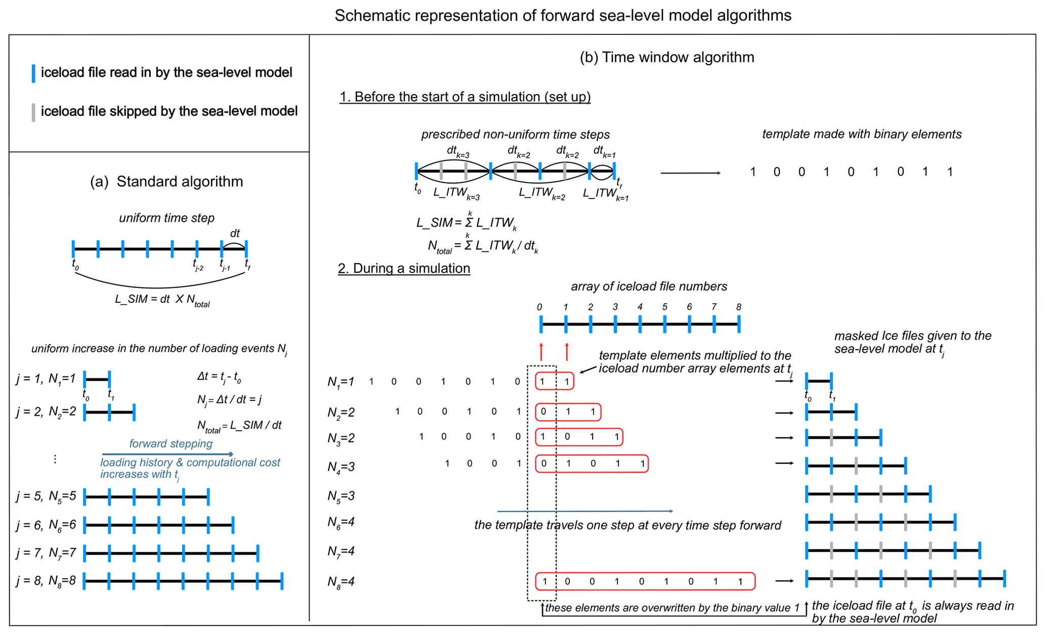
Figure 1 Schematic diagram of standard and time window algorithm in forward sea-level modelling. (a) The standard forward model algorithm in which the surface (ice sheet and ocean) loading history is captured in uniformly discretized temporal resolution. (b) The time window algorithm that captures the details of the loading history in non-uniformly discretized temporal resolution. The user assigns k number of internal time windows, each of which has a total length of L_ITW_k and internal time steps of size dt_k. The ice load files shown as blue vertical bars are multiplied by a template element with a value “1” (considered by the sea-level model), and grey bars are multiplied by “0” (ignored by the sea-level model).

Figure 1a represents the standard forward sea-level model algorithm (Gomez et al., 2010) in which the time interval dt between each time step of the ice history is uniformly fixed throughout a simulation. By the end of the simulation, the total number of ice history steps (N_j) considered in the calculation across the final time step from $t_{j=f-\mathrm{1}}$ to t_j=f is simply the length of the simulation (L_SIM) divided by the prescribed time interval (dt). Thus, the number of time steps in a simulation increases either by performing a longer simulation (i.e., larger L_SIM) or increasing the temporal resolution (i.e., smaller dt) of a simulation, and the CPU time increases quadratically.

Figure 1b shows the time window scheme that we developed to save computation time in the sea-level model. This algorithm allows users to assign non-uniform time steps across simulations by dividing the simulations into as many as four time intervals, which we call “internal time windows (ITWs)”. (We note that our model can be easily modified to adopt a greater number of internal time windows, but we found that four is sufficient for a range of applications such as long paleo-simulations and short simulations with rapidly retreating ice sheets.) During set-up, users define the internal time window length (L_ITW_k) and temporal resolution (dt_k) such that each L_ITW_k is divisible by dt_k and each dt_k is divisible by the finest temporal resolution of the simulation time window (dt_k=1; i.e., the coupling time between a dynamic ice-sheet model and the sea-level model. As an example, notice dt₃ and dt₂ are 3 times and 2 times larger than dt₁ in the time window schematic shown in Fig. 1b). In addition, the sum of all L_ITW_k values must be equal to the total length of a simulation, L_SIM. The algorithm then generates a template mask of binary values to resolve the prescribed non-uniform time steps (see Fig. 1b-1). It also creates an array of iceload file numbers that, by convention, start at 0 and increment by 1 each time step forward. When the simulation begins (i.e., takes one step forward from j=0 to j=1), the first two elements of this array (iceload files “0” and “1”) overlap the last two elements of the binary template (see the top red box in Fig. 1b-2). Overlapping elements are multiplied together to generate masked iceload history files for the sea-level model to read in at a given time step. The sea-level model only reads in those ice files masked with a binary value of 1. However, to ensure that the solid Earth retains the memory of the initial loading, the sea-level model always reads the initial iceload file (see the dotted box and resulting masked iceload files in Fig. 1b-2).

At every simulation step j>1, the template marches forward by one element relative to the iceload file array, and the multiplication process repeats followed by the sea-level calculation. Our algorithm starts filling in the first internal time window to its prescribed length (L_ITW₁), followed by the other internal windows in order (L_ITW_k for $k=\mathrm{2},\mathrm{3},\mathrm{4}$). By the end of the simulation, the time window grows to the fully prescribed profile (see the j=8 result in Fig. 1b-2).

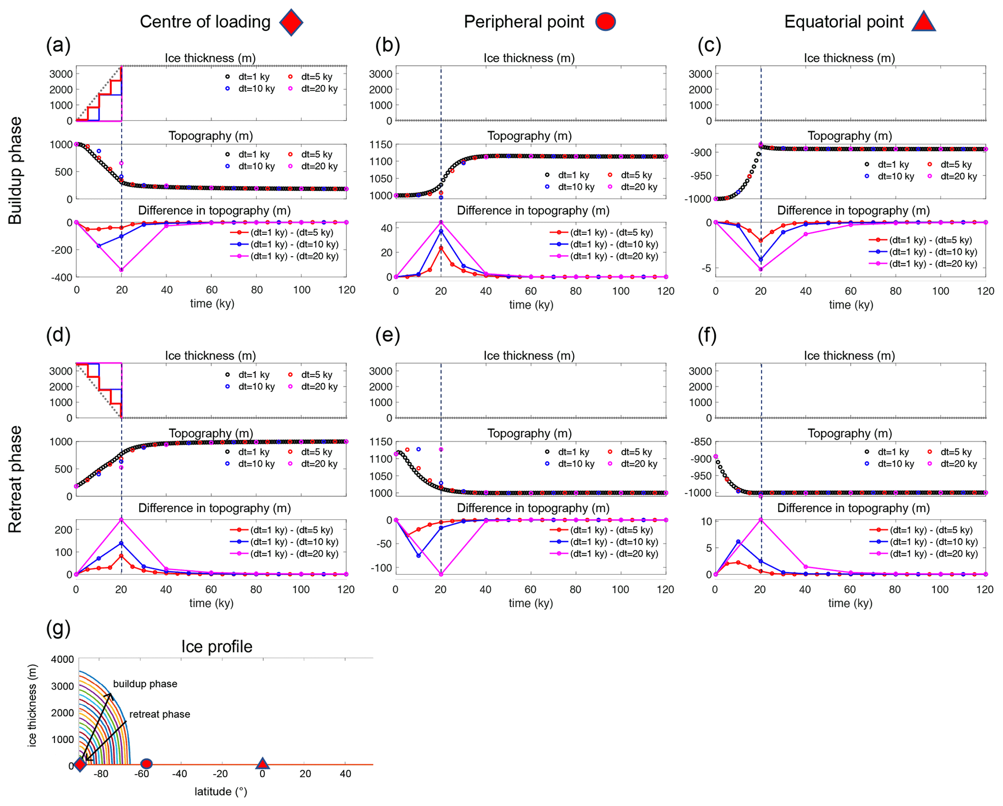
Figure 2 The sensitivity of predicted topography (sea level) changes to the temporal resolution (dt) of the sea-level model and ice profile adopted in this experiment. (a–f) Results of idealized simulations in which input ice history evolves at a uniform rate in an axis-symmetric dome shape during a build-up phase (a–c) and a retreat phase (d–f) at the centre of loading (first column), peripheral point (second column) and far-field equatorial point (third column). In each panel, the top frame shows ice thickness in meters, the middle frame shows the elevation of topography in meters from simulations that incorporate the uniform time stepping of dt=1 kyr (black dots), 5 kyr (red dots), 10 kyr (blue dots) and 20 kyr (magenta dots), and the bottom frame shows differences in predicted topography from the simulation with the benchmark resolution (black dots in the middle panel, dt=1 kyr) and coarser temporal resolution (red, blue and magenta dots in the middle panel). Dashed vertical lines at 20 kyr mark the timing at which the ice stops loading. The staircase-like solid lines in (a) and (d) represent the step function of ice loading change in respective simulations. (g) Schematic of the half-cross section of the ice profile incorporated in the idealized simulations in the Southern Hemisphere.

Overall, this time window algorithm limits the increase in the number of ice history steps with simulation length or temporal resolution, improving the computational efficiency of the sea-level model calculations (compare N_j values in Fig. 1a, b-2). The time window algorithm also enables the sea-level model to capture both short- and long-term interactions between ice sheets, sea level and the solid Earth in coupled ice-sheet–sea-level simulations.

In the next section, we perform a suite of stand-alone sea-level simulations and coupled ice-sheet–sea-level simulations to test the sensitivity of model results to the temporal resolution of the 1D sea-level model, which incorporates radially varying Earth structure. The elastic and density profiles of the Earth structure are given by the seismic model PREM (Dziewonski and Anderson, 1981). For mantle viscosity, we adopt a lithospheric thickness of 120 km and upper-mantle viscosity of 5×10²⁰ Pa s and lower-mantle viscosity of 5×10²¹ Pa s in Sect. 3.1–3.3.1. For Sect. 3.3.2 in which we perform simulations over Antarctica, we adopt the best-fitting radially varying Earth model from Barletta et al. (2018), characterized by a lithospheric thickness of 60 km and upper-mantle viscosities of ∼ 10¹⁸–10¹⁹ Pa s. Ice history inputs are described in each section with reference to corresponding figures. In all simulations, we perform sea-level calculations using a spherical harmonics expansion up to degree and order 512. For coupled ice-sheet–sea-level simulations, we couple the 3D PSU ice-sheet–ice-shelf model (Pollard and DeConto, 2012) to the sea-level model. The flux across the grounding line is parameterized following Schoof (2007). The ice-sheet model does not include the marine ice-cliff instability (MICI) mechanism. Readers are referred to Han et al. (2021) and DeConto et al. (2021) for more detailed set-ups for the Northern Hemisphere and Antarctic Ice Sheet simulations.

3 Results

3.1 Sensitivity of sea-level model outputs to temporal resolution

Before exploring the sensitivity of coupled ice-sheet–sea-level modelling to the model temporal resolution in the following subsection, we begin by testing the sensitivity of stand-alone standard sea-level modelling to the temporal resolution (Fig. 1a). We generate an idealized axis-symmetric input ice history based on the equation for an equilibrium ice surface profile for viscous ice provided in Cuffey and Paterson (1969, The Physics of Glaciers), with the ice sheet centred at the South Pole (Fig. 2g). We note that the ice thickness at the centre of loading (as shown in the top frames of Fig. 2a, d) changes linearly, but the actual volume change is non-linear because of the changes in the ice-sheet extent; the volume change across one time step is greater when the ice sheet is more extensive. The initial topography for the ice growth phase is idealized such that its elevation is 1000 m between 60–90^∘ S and −1000 m (ocean with a depth of 1000 m) everywhere else. In Fig. 2, we consider predicted changes in topography at three locations: a location at the centre of loading (90^∘ S), near the periphery of the ice sheet at its maximum extent (65^∘ S, where the peripheral bulge formed around the ice sheet is largest) and in the far field at the Equator (0^∘ latitude). We begin by discussing the general behaviour of topography at these sites in benchmark simulations performed at a temporal resolution of 1 kyr (shown by the black dots in Fig. 2).

Figure 2a–c show results from build-up-phase simulations at near- and far-field locations. The ice-sheet thickness and extent grow over 20 kyr at a uniform rate at the centre and the edge of the loading to the thickness of 3500 m (top frame of Fig. 2a) and the extent reaching latitude 65^∘ S. In response, the topography subsides at the centre of loading (middle frame of Fig. 2a) and uplifts at the peripheral point (middle frame of Fig. 2b). The far-field equatorial site experiences a decrease in sea level (increase in topography) as water from the ocean becomes locked up on land (middle frame of Fig. 2c).

Figure 2d–f show results over a 20 kyr long retreat phase. The initial topography for these simulations is adopted from the final topography modelled in the benchmark build-up-phase simulation with dt=1 kyr (i.e., black dots in the middle frame of Fig. 2a). As the ice sheet retreats, the topography uplifts at the centre of the ice load (middle frame of Fig. 2d) and subsides at the location peripheral to the ice (middle frame Fig. 2e), and the far-field site experiences a rise in sea level (middle frame of Fig. 2f).

Next, we compare simulations performed at lower temporal resolutions of 5, 10 and 20 kyr to our benchmark simulations at 1 kyr resolution. Though all of the simulations capture the main characteristics of deformation at each location, the magnitude of the deformation during both the ice-sheet build-up and retreat phases at all three locations decreases with decreasing temporal resolution (i.e., larger dt). For example, when comparing the 5 kyr resolution simulation to the benchmark simulation for the build-up phase (red line in the bottom frame of Fig. 2a), the subsidence beneath the ice during ice growth is reduced by up to 51.7 m. Likewise, the simulations with 10 and 20 kyr resolution (blue and pink lines) underestimate the subsidence by up to 173 and 349 m, respectively. The underestimation is due to the different timing of the applied load in each simulation; as shown by the step function, ice loading increases in the top frames of Fig. 2a and d, and simulations with coarser temporal resolution have delayed increases in ice loading. For example, the loading change for the 5 kyr resolution simulation is applied in two steps at 5 and 10 kyr, while in the 10 kyr resolution simulation, the full load is applied once at 10 kyr. The latter thus does not capture the viscous signal due to the loading that takes place before 10 kyr. (We note that this result is the direct consequence of the linear viscoelastic relaxation process of the solid Earth. The result also depends on the timing of ice loading changes. That is, a viscous signal would be evident if the ice loading change was applied at the start of each time step rather than the end of the time step. This issue has been discussed in the glacial isostatic adjustment model inter-comparison and benchmarking efforts; e.g., Barletta and Bordoni, 2013.) Then, these maximum differences (“errors”) and the spread of the errors decrease gradually towards zero with time (the bottom frames of Fig. 2a–f). For all simulations, the errors in total topography change become less than 1 % of the total subsidence (801 m) in the benchmark simulation by 60 kyr (i.e., within 40 kyr after the completion of loading/unloading event at 20 kyr).

Overall, the idealized loading simulations show that sea-level model outputs are sensitive to the model temporal resolution. This is because the timing of ice loading is different with different temporal resolutions. The sensitivity at a location depends on its setting (above or below sea level), the size of ice loading changes and the distance (near field or far field) to the changing ice load. However, the sensitivity at all sites decreases with time after the ice loading event. These results suggest (as expected from the literature on the viscoelastic response of the Earth to surface loading; e.g., Peltier, 1974) that higher-resolution information about ice cover changes is required for the ice history immediately prior to the current time step in a simulation, and lower resolution will suffice for earlier ice cover changes. The specific temporal resolution required will depend on both the rates of change of the ice cover and the Earth's viscosity structure, which we explore in two contrasting examples in Sect. 3.3.

3.2 Sensitivity of modelled ice-sheet dynamics to temporal resolution of a coupled sea-level model

This section explores how the differences in predicted sea-level change due to temporal resolution of the input ice history discussed in the previous section impact ice dynamics in coupled ice-sheet–sea-level model simulations. To do this, we perform a suite of coupled simulations over the Northern Hemisphere through the last glacial cycle (125 kyr) incorporating different sizes of uniform time steps with the standard algorithm (Fig. 1a) and non-uniform time steps applying the time window algorithm (Fig. 1b). We employ the PSU 3D dynamic ice-sheet model by Pollard and DeConto (2012) and adopt the same set of ice model parameters (e.g., climate forcing, basal friction, spatial and temporal domain and resolutions) used in the simulations from the main text of Han et al. (2021). The ice-sheet model has a stand-alone time step of 0.5 years. We note that the coupling interval over which the ice-sheet model and sea-level model exchange their outputs (i.e., ice thickness and topography, respectively) corresponds to the size of the most recent time step within the sea-level model (i.e., dt₁ in Fig. 1b).

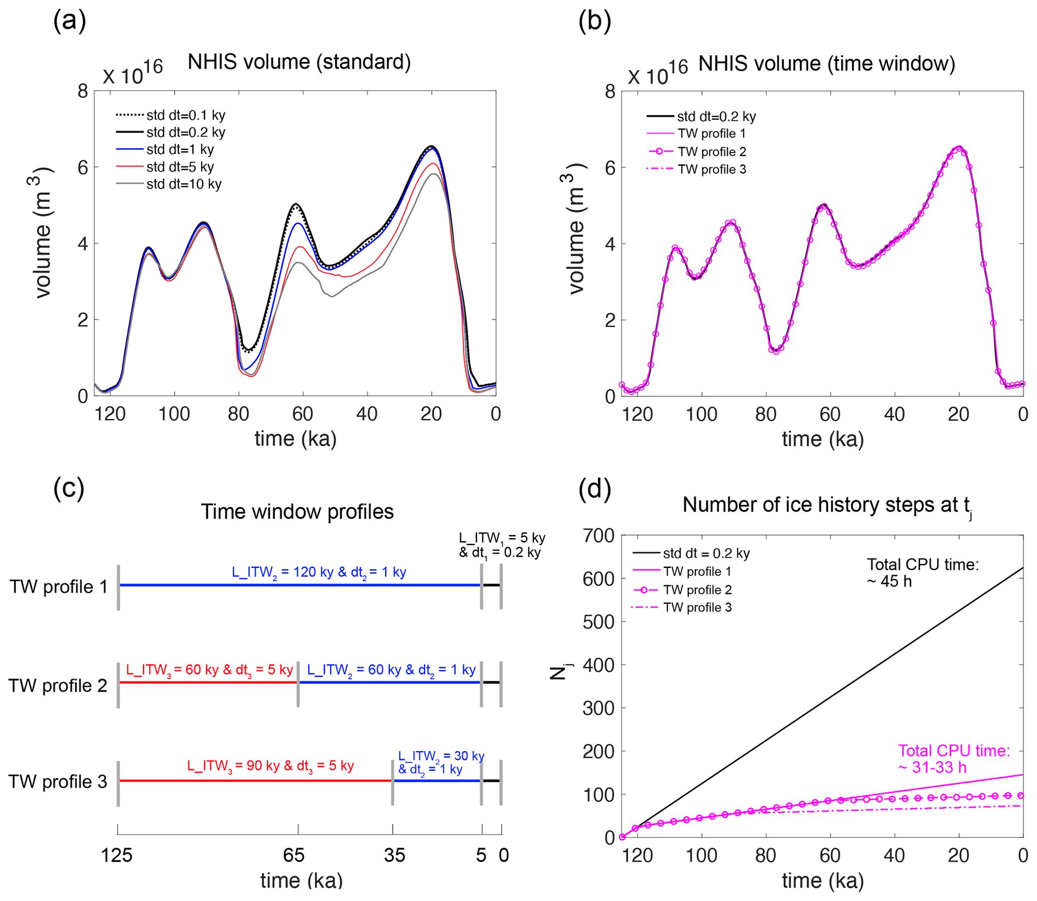
Figure 3 Modelled Northern Hemisphere ice-sheet volume through the last 125 kyr from ice-sheet–sea-level coupled simulations. Volume variations in Northern Hemisphere ice sheets simulated in the coupled ice-sheet–sea-level simulations that incorporate (a) “standard”, uniform time stepping (and thus coupling time interval) of 0.1 kyr (dotted black line), 0.2 kyr (black line), 1 kyr (blue line), 5 kyr (red line) and 10 kyr (grey line). (b) Non-uniform time intervals assigned by the time windows of three different profiles (magenta lines) as schematically shown in (c); TW profile 1 applies two internal time windows, L_ITW₁ and L_ITW₂, each of which covers 5 and 120 kyr over the entire simulation with dt₁=200 years and dt₂=1 kyr. TW profile 2 applies three internal time windows, L_ITW₁–L_ITW₃, each of which covers 5, 30 and 90 kyr with dt₁=0.2, dt₂=1 and dt₃=5 kyr, and TW profile 3 also applies three internal time steps, each of which covers 5, 60 and 60 kyr with dt₁=0.2, dt₂=1 and dt₃=5 kyr, respectively. Note that all three profiles assign the first internal time window (L_ITW₁) to a 5 kyr length with the internal time step (dt₁) of 200 years. (d) The number of ice history steps (N_j) that the sea-level model considers at every time step t_j. Note that the x axis represents thousand years before present (ka) such that 0 ka is the present day.

Figure 3a demonstrates that the simulations with a higher temporal resolution (i.e., smaller “dt” in the sea-level model and thus more frequent exchange of outputs between the ice-sheet model and the sea-level model) generally yield a higher volume of modelled Northern Hemisphere ice sheet (NHIS) during the time between ∼ 80–20 ka. Differences in ice volume between the simulations start diverging around 80 ka and persist until the Last Glacial Maximum (20 ka) in the model time. The difference in sea-level-equivalent ice volume is up to 11.6 m between the simulations with time intervals of dt=0.1 kyr and dt=1 kyr at 80 ka (compare dotted black line and blue line in Fig. 3a). Spatially, the differences occur mainly in the Laurentide Ice Sheet in North America (which we do not show in the figure). A lower temporal resolution of the ice history during the Laurentide Ice Sheet retreat before 80 ka leads to less uplift of the bedrock beneath the continental ice sheet (which is more sensitive to deformational feedback than to sea-level feedback), keeping the ice surface at a lower (and thus warmer) elevation in the atmosphere. This lower ice elevation causes more intense deglaciation of the Laurentide Ice Sheet. It also prohibits the ice sheet from growing large during build-up phases later (the role of deformational effects on ice-sheet dynamics is discussed in detail in Han et al. 2021). Furthermore, the NHIS volume fluctuation becomes less smooth when the coupling time interval is increased to dt=5 kyr and dt=10 kyr (red and grey lines in Fig. 3a). We presume that this is because a larger change in bedrock height over a longer coupling time causes the ice-sheet model to respond more strongly. These results suggest that if the model is only capable of assigning a uniform temporal resolution, Northern Hemisphere coupled simulations over the last glacial cycle require a resolution of hundreds of years to maintain the coupling time interval short enough to accurately capture the interactions between the ice sheets, bedrock elevation and sea level during deglacial phases (see the divergence of the non-black lines after the strong deglaciation at ∼ 80 ka in Fig. 3a.)

While we might expect that the computation time would always increase with higher temporal resolution in the case of uniform time stepping, it is interesting to note that the 10 kyr time-step simulation took an hour longer than the 5 kyr case. This is because in the former simulation, the ice model took longer to converge to a solution (Pollard and DeConto, 2012) because of infrequent and dramatic bedrock changes provided by the sea-level model (as hinted by the unstable fluctuation in the ice volume; grey line in Fig. 3a). Finally, while there are very small differences in predicted ice volume between the dt=0.2 kyr and dt=0.1 kyr simulations (black and dotted black lines in Fig. 3a), the total CPU time increases from ∼ 45 to ∼ 98 h, and we choose dt=0.2 kyr as an adequate choice of coupling time for glacial cycle simulations.

In Fig. 3b, we apply the time window algorithm to the coupled glacial-cycle simulation rather than adopting uniform temporal resolution in the ice history. We perform three simulations with different time window profiles illustrated in Fig. 3c. All simulations incorporating the time window predict well the ice volume changes of the standard simulation with the uniform time stepping of 0.2 kyr (see the magenta lines and the black line overlapping in Fig. 3b). This indicates that the coupled simulation results are relatively insensitive to the specific choices for the time window profile for the past time steps compared to the choices for the recent and current time steps of the simulations. In the standard simulation, the number of ice history files that the sea-level model needs to read in at a given time step increases linearly with time (black line in Fig. 3d). In contrast, with the time window algorithm, it increases linearly only for the first 5 kyr (125–120 kyr), which is the length of the first internal time window (L_ITW₁=5 kyr), and is then nearly capped, increasing by one intermittently when transitioning from one internal time window to the next (pink lines in Fig. 3d). The number of files is capped at 145 files in time window profile 1, at 97 files in profile 2 and at 73 files in time window profile 3. In all cases, the time window algorithm allows for faster computation while maintaining precision (Fig. 3b, d), and the total CPU time is reduced by ∼ 12–14 h (Fig. 3d).

In this subsection, we have shown that a coarse temporal resolution (e.g., dt=1 kyr or longer) causes less precise coupled ice-sheet–sea-level simulation results by taking the last glacial cycle as an example. We have also demonstrated how the time window algorithm can be used in coupled simulations to maintain the precision of the modelled topography changes and ice-sheet dynamics while significantly reducing the computational cost compared to simulations with the standard algorithm. In the same way, the time window algorithm can be applied to other coupled simulations that are otherwise infeasible. In the next subsection, we derive time window profiles that are suitable for two-glacial-cycle global ice-sheet simulations and future projections of rapidly retreating Antarctic Ice Sheet.

3.3 Derivation of time window profiles for different applications

In this section, we apply the time window algorithm in the sea-level model to two contrasting examples. First, we consider sea-level changes in response to the evolution of global ice sheets over the last two glacial cycles (240 kyr) modified from Han et al. (2021). We also consider a simulation of the rapid future retreat of the West Antarctic Ice Sheet in the coming centuries taken from DeConto et al. (2021). West Antarctica is known to have an upper-mantle viscosity up to several orders of magnitude lower than the global average and thus the shorter relaxation timescale of the solid Earth (Barletta et al., 2018; Lloyd et al., 2020; Nield et al., 2014). This combination of higher rate of ice-sheet evolution and solid Earth response requires higher temporal resolution in sea-level calculations. For each scenario, we perform a suite of stand-alone sea-level simulations in which we vary the time window parameters (i.e., L_ITW_k and dt_k; Fig. 1) and compare them to a benchmark simulation with uniform high-resolution time stepping to systematically arrive at a preferred choice of a time window profile. Here we note that the experiments are first done in stand-alone sea-level simulations (i.e., ice cover is prescribed rather than provided by a dynamic ice-sheet model) partly because the benchmark coupled simulation for the two glacial cycles NH simulation is infeasible without the time window algorithm. After we derive the respective time window profiles, we perform a suite of coupled future WAIS–sea-level simulations to test the performance of the time window profile derived in the section.

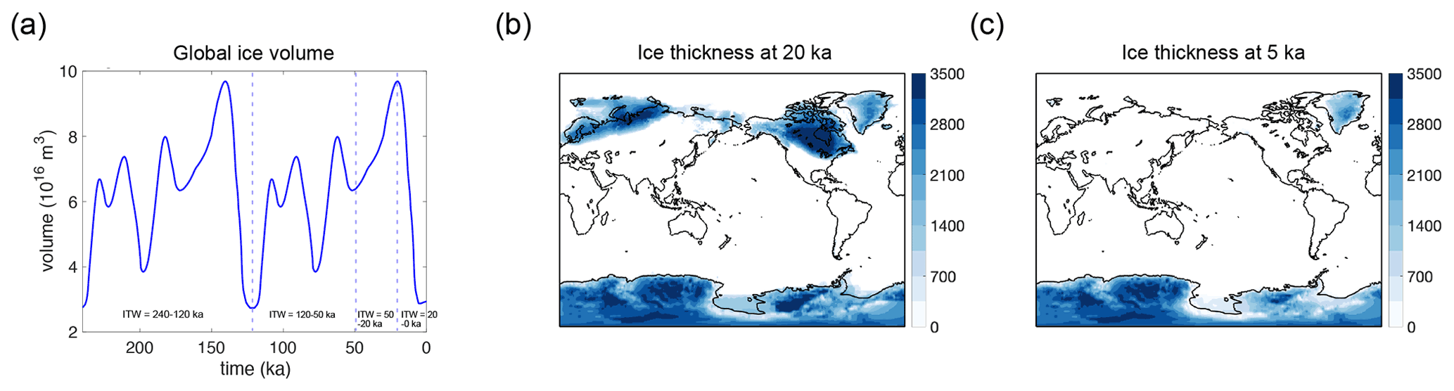
Figure 4 Changes in global ice-sheet volume and thickness and in the 240 kyr simulation. (a) Global volume variations through the last 240 kyr. Vertical dashed lines mark the internal time windows. (b, c) Snapshots of ice thickness at (b) 20 ka and (c) 5 ka.

3.3.1 Application to global ice cover changes over the last two glacial cycles

Figure 4 shows ice volume changes over the last 240 kyr and snapshots of the maximum and minimum extent of global ice cover adopted from a coupled ice-sheet–sea-level model simulation in Han et al. (2021). The original simulation covers the last glacial cycle (125 ka). To extend our ice history input to cover two glacial cycles, we first take the ice history for 120 ka from the original simulation (Han et al. 2021), then repeat this ice history to cover an additional glacial cycle going back to 240 ka. We replace the ice history between 125–120 ka with the ice history between 120–115 ka. This is to make the ice volume curve continuous at the last interglacial. Globally, it includes ice-cover changes predicted with the dynamic PSU ice-sheet model (Pollard and DeConto, 2012) in the Northern Hemisphere and Antarctic ice cover changes taken from the ICE-6G_C ice history model (Argus et al., 2014; Peltier et al., 2015). We note that the goal of this experiment is not to produce an accurate glacial history but to produce a sample long timescale – a global ice history that contains the spatiotemporal detail provided by a dynamic ice-sheet model.

To explore the choice of time window parameters for this global glacial-cycle scenario, we first perform a standard sea-level simulation in which we assign a uniform temporal resolution of 0.2 kyr throughout the 240 kyr simulation. We take this simulation as our benchmark and then perform a suite of simulations in which we systematically vary the temporal resolution (dt) of internal time windows (ITWs) that cover the periods 240–120, 120–50 and 50–20 ka in the simulation (see the internal time windows marked by dashed lines in Fig. 4a). We choose these internal time windows based on the timing of ice volume variations and the results of our idealized tests in Sect. 3.1. That is to say, our first internal time window covers the last deglaciation, the next covers the preceding growth phase in the simulation then the rest of the glacial cycle back to the last interglacial, and finally the entire penultimate glacial cycle. We note that in the absence of knowing the specific details of the ice cover changes a priori (as in coupled model simulations), the internal time windows may also be set based on the timing of the climate forcing that serves as input to the model. Sensitivity tests (not shown here) varying the internal time window lengths to account for potential offsets between the timing of climate forcing and ice-sheet response indicate that the timing of these internal time windows need not be set very precisely, with less sensitivity for earlier ice history.

Figure 5 Time window profiles, RMSE in predicted topography, the number of loading events considered at t_j (N_j) and the total CPU times it has taken for the sea-level model to perform calculations at time step t_j in the global simulations through the last 240 kyr. Results from the simulations in which we explore the internal time windows that cover the periods between (a–d) 240–120 ka, (e–j) 120–50 ka and (i–l) 50–20 ka. Note that the benchmark simulation assigns a uniform time-step size of 0.2 kyr throughout the simulation.

We explore each internal time window in turn by varying the internal time step (i.e., temporal resolution dt), starting from the earliest and fixing the temporal resolution at 0.2 kyr for all periods beyond the internal time window. Then, we compare the total CPU time (Fig. 5d) and the precision of our results by calculating the root mean squared error (RMSE) in predicted topography at a given time step relative to the benchmark simulation. The RMSE is calculated based on the following expression:

$$\mathrm{\text{RMSE}}\left(t_j\right)=\sqrt{{\displaystyle \frac{\mathrm{1}}{N}}\sum _l^{L=\mathrm{512}}\sum _m^{M=\mathrm{1024}}\left[T\right(t_j,l,m{)}_{\text{std}}-T(t_j,l,m{)}_{\text{tw}}{]}^{\mathrm{2}}},$$

where j represents the time index, N represents the number of grid points (in our case, 512 × 1024 for the Gauss–Legendre sea-level model grid), and $T(t_j,l,m{)}_{\text{std}}$ and $T(t_j,l,m{)}_{\text{tw}}$ represent predicted topography at time t_j from the standard simulation and the time window simulation. Once we choose a preferred temporal resolution for the internal time window based on the calculated RMSE and CPU time, we move on to explore the next internal time window, and we repeat the same procedure.

We start by exploring the internal time window covering the earliest period between 240–120 ka (see the purple bar in Fig. 5a). Varying the internal time step between 5–40 kyr for this period (Fig. 5a–d), the RMSE in predicted topography is zero for the first 120 kyr (Fig. 5b) because all four time window profiles assign a temporal resolution of 0.2 kyr for the first 120 kyr of the simulation, which is the same time resolution as in the benchmark simulation (as shown in the black bar indicating 120–0 ka in Fig. 5a). RMSE then starts to increase for all simulations once the simulations proceed past 120 ka. The simulations with an internal time step of 20 and 40 kyr show noticeably greater RMSE than the simulations with a smaller internal time step of 5 and 10 kyr, both of which have RMSE below 0.2 m throughout the last glacial cycle except at 5 ka when it rises to 0.35 m. The fluctuations in the RMSE curves are mainly associated with the sea-level model not capturing the highs and lows in the input ice history. Taking the simulation with the internal time step of dt=40 kyr (blue line in Fig. 5b) as an example, the RMSE peaks at around 40 ka because the sea-level model only captures snapshots of ice at their local minimum (at 240, 200 and 160 ka) and misses multiple glacial peaks at 230, 210 and 190 ka within those periods (Fig. 4a).

Figure 5c and d show the total number of ice history steps considered and the cumulative CPU time it has taken for the sea-level model to perform calculations at time step t_j in the standard simulation (grey line) and all other simulations that incorporate the time window parameters (non-grey lines). In the standard simulation, CPU time increases quadratically with a linear increase in total number of ice history steps that goes up to 1200 (and the total CPU time accumulates to ∼ 58.4 h). The total number of ice history steps starts flattening for the simulations with a time window (coloured lines) at 120 ka, resulting in the reduction in the CPU time to ∼ 46.8–50.3 h. We note that the CPU time starts diverging earlier than 120 ka, and this is because measured CPU times fluctuate by 10 %–17 % even with the same CPU (Intel Gold 6148 Skylake at 2.4 GHz). Based on these results, we choose an internal time step of 10 kyr for the first internal time window (240–120 ka) and proceed to explore the internal time steps for the next internal time window between 120–50 ka.

Figure 5e–h show the results of simulations in which we vary the internal time step for the period between 120–50 ka (purple bar in Fig. 5e) while fixing the first period from 240–120 ka to dt=10 kyr. Here we see that the simulation with temporal resolution of 1 kyr (red line in Fig. 5f–h) has comparable RMSEs to the RMSEs in the simulation with temporal resolution of 0.2 kyr for this internal time window (black line in Fig. 5f–h) with comparably low computing time to the other lower temporal resolution simulations (pink and blue lines in Fig. 5f–h). We also note that the peak in RMSEs at ∼ 5 ka is related to the internal time window covering 240–120 ka with dt=40 kyr not capturing the intense deglaciation phase at 140–120 ka (see Fig. 4a). The total CPU time is reduced to ∼ 29.7 h in this case, a 49 % reduction compared to the benchmark simulation for this internal time window (compare red and grey line in Fig. 5h). Hence, we adopt a temporal resolution of 1 kyr for this period.

Finally, Fig. 5i–l explore the effects of varying the size of the internal time step for the period between 50–20 ka (purple bar in Fig. 5i). Based on the above discussion, the size of the internal time steps for the periods 240–120 ka and 120–50 ka are fixed at dt=10 and 1 kyr, respectively. We arrive at the final preferred time window profile by identifying dt=0.4 kyr (red line in Fig. 5h–i) as a preferred internal time step for this internal time window. This profile keeps the RMSEs in output topography below 0.4 m throughout the entire simulation. The total CPU time is reduced to ∼ 26.9 h, a 54 % reduction compared to the benchmark with uniform time stepping of 0.2 kyr. We note that the CPU times shown in Fig. 5 are based on stand-alone sea-level simulations only. This time window algorithm is designed for sea-level calculations performed within a coupled ice-sheet–sea-level simulation, and computation time will be similarly reduced in this context. Moreover, the reduction will grow for longer simulations as the CPU time in the standard simulation will increase quadratically whereas the time window simulation will suppress the rapid growth.

3.3.2 Application to future Antarctic Ice Sheet changes

In this section, we develop a time window profile for the application of simulating future West Antarctic Ice Sheet (WAIS) collapse based on the same methodology that we use for the global glacial-cycle scenario in the previous subsection. For the ice history model, we adopt a simulation of future AIS evolution from DeConto et al. (2021) in which marine sectors of the WAIS collapse over hundreds of years. The simulation does not include ice shelf hydrofracture and ice cliff instability (Pollard et al., 2015). For the Earth model, we adopt a profile of thin lithosphere and low mantle viscosity as described in “Methods” (Sect. 2). The rapid retreat of the WAIS and the weak solid Earth structure together suggest that ice-sheet–solid-Earth interactions may need to be captured at decadal timescales or less. We therefore perform our benchmark sea-level simulation for this scenario with a uniform (standard) temporal resolution of dt=1 year. We also perform additional standard simulations with a coarser temporal resolution of dt=5, 10 and 50 years for comparison. We then perform a suite of simulations in which we vary the temporal resolution between dt=5–50 years within the four internal time windows shown in Fig. 6a (also see the purple bars in Fig. 7a, e and i).

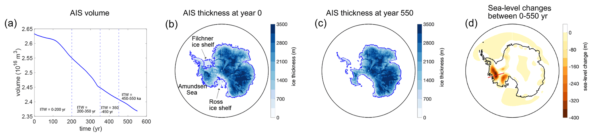
Figure 6 Changes in Antarctic Ice Sheet volume and thickness over 550 years from DeConto et al. (2021) and associated total sea-level changes predicted in a stand-alone (uncoupled) sea-level simulation. (a) AIS volume variations through 550 years. Vertical dashed lines mark the internal time windows. (b, c) Snapshots of ice thickness (blue) and grounding lines (blue contour lines) at (b) 0 years and (c) 550 years. (d) Total sea-level changes between 0–550 years associated with the ice loading changes between 0–550 years. Note that the regions (in yellow and red) that show negative sea-level changes are where sea level has fallen because of solid Earth uplift and the drawdown of sea surface height associated with ice mass loss. The red line represents a cross section perpendicular to a grounding line in the West Antarctic region where the most intense sea-level change (fall) happens (see also Fig. 8).

Figure 6 shows AIS volume changes and maps of the AIS thickness at the beginning and end of the 550-year simulation beginning in 1950 CE from Deconto et al. (2021) along with total sea-level change in Antarctica across the simulation predicted from our benchmark stand-alone sea-level simulation. Marine-grounded ice sheets in the Amundsen Sea Embayment in West Antarctica retreat completely along with the Ross and Filchner–Ronne ice shelves (Fig. 6b–c), and strong sea-level fall occurs in the region (shown in dark orange in Fig. 6d). Accordingly, in these marine sectors, it becomes important to capture deformation at the grounding line accurately within coupled model simulations. In the remainder of this section (Figs. 7–10), we derive a time window profile based on global RMSE and then test the performance of the chosen time window at capturing deformation and the ice-sheet profile across the grounding line in the region.

We start by finding a preferred internal time step (i.e., temporal resolution) for the period between 0–200 years of simulation time (Fig. 6a; also marked as a purple bar in Fig. 7a), during which the WAIS starts retreating, and the rate of retreat starts accelerating just after 100 years. We leave the rest of the 200–550-year period at dt=1 year, which is the same as in the benchmark simulation (see the black bar in Fig. 7a). Figure 7b shows that, as the time window marches forward, RMSEs in predicted topography compared to the benchmark simulation start to increase only after 350 years of the simulation time. The RMSEs remain smaller than 10 cm for simulations with an internal time step of 10 and 25 years (red and magenta lines in Fig. 7b) and below 0.85 cm with an internal time step of 5 years (black line in Fig. 7b). The number of ice history steps (N_j) that the sea-level model considers at time step t_j starts diverging after 350 years. At the last time step of the simulation, the benchmark simulation considers 550 ice history steps, while N_j considered for the simulations with an internal time step dt=5–50 years are reduced by ∼ 29 %–36 %, respectively (Fig. 7c). The total CPU times are reduced by ∼ 4 %–8 %, from ∼ 17 h with the standard simulation to between ∼ 15.6–16.3 h for the others (Fig. 7d). We choose dt=5 years as an appropriate internal time step for the period between 0–200 years (the black lines in Fig. 7b–d), which minimizes the RMSE with comparable CPU time to the other simulations.

Next, we explore the period 200–3 years (Fig. 7e–h) during which the most intense ice loss occurs (Fig. 6a). The simulations with internal time steps of 25 and 50 years show a noticeable increase in RMSEs compare to those with a smaller internal time step (compare the blue and magenta lines to red and black lines in Fig. 7f). Comparing the simulations with a finer resolution of dt=5 years (black line) and coarser resolution of dt=50 years (blue line), the former considers a total of 270 ice history steps, and the computation time is ∼ 11.5 h, which is 27 more ice history steps and ∼ 2 h longer computation time than the latter simulation. Since the simulation with the fine internal time step of 5 years is entirely feasible, and the RMSE in predicted topography is below 0.04 m, we choose dt=5 years (black lines in Fig. 7f–h) as our temporal resolution for this period.

Finally, Fig. 7i–l show the results of exploring the temporal resolution for the period between 350–450 years. Again, the simulation with the internal time step of 5 years outperforms the other simulations that have a coarser temporal resolution, keeping the RMSEs in predicted topography below 0.07 m throughout the simulation (black line in Fig. 7j) without a significant increase in computation time and ice history steps compared to the other coarser simulations (Fig. 7k). The total computing time for the 5-year simulation is ∼ 8.5 h (Fig. 7l), which is a ∼ 50 % reduction from the computing time of the benchmark simulation (∼ 17 h) and only ∼ 3 %–6 % longer than the other simulations (dt=10, 25 and 50 years). Thus, we arrive at an appropriate time window profile (black line shown in Fig. 7j–l).

Having chosen the time window profile for the future AIS retreat scenario, we compare predicted topography from this time window simulation to that from the standard simulations that incorporate coarser uniform temporal resolutions of 5, 10 and 50 years. Figure 8 shows snapshots of ice thickness and predicted topography at model times 250, 350 and 550 years relative to 0 years along the cross section in Amundsen Sea Embayment across which the grounding line retreats during the simulations (shown by the red line in Fig. 6d). Figure 8a–c show a rapid retreat of the marine-based West Antarctic Ice Sheet on a reverse-sloped bed between 250–550 years and substantial bedrock uplift in response to the ice unloading. When the ice-sheet retreat and associated topography changes are small in the first 250 years of the simulation (see the solid blue and dotted blue lines in Fig. 8c), the differences in predicted topography from standard simulations with resolutions of 5–50 years (blue, red and magenta lines) compared to the benchmark 1-year simulation reach up to 10 m. The spread of the differences increases even more as the retreat becomes more intense after 250 years (see the changes in the differences from Fig. 8d to e). By 350 years, after ∼ 330 km of grounding line retreat along the cross section (solid blue to dashed blue lines in Fig. 8b), the standard simulation that incorporates dt=50 years shows up to 80 m of difference in predicted topography compared to the benchmark simulation. The standard simulation that incorporates a relatively fine resolution of 5 years still shows topographic differences in the grounding zone reaching a maximum of 5 m during the simulation (red line in Fig. 8e). Meanwhile the maximum difference in topography in the simulation adopting the time window algorithm is less than 0.1 m by 350 years and less than 1 m by 550 years, or 0.24 % of the total deformation (which goes up to 391 m by the end of the simulation).

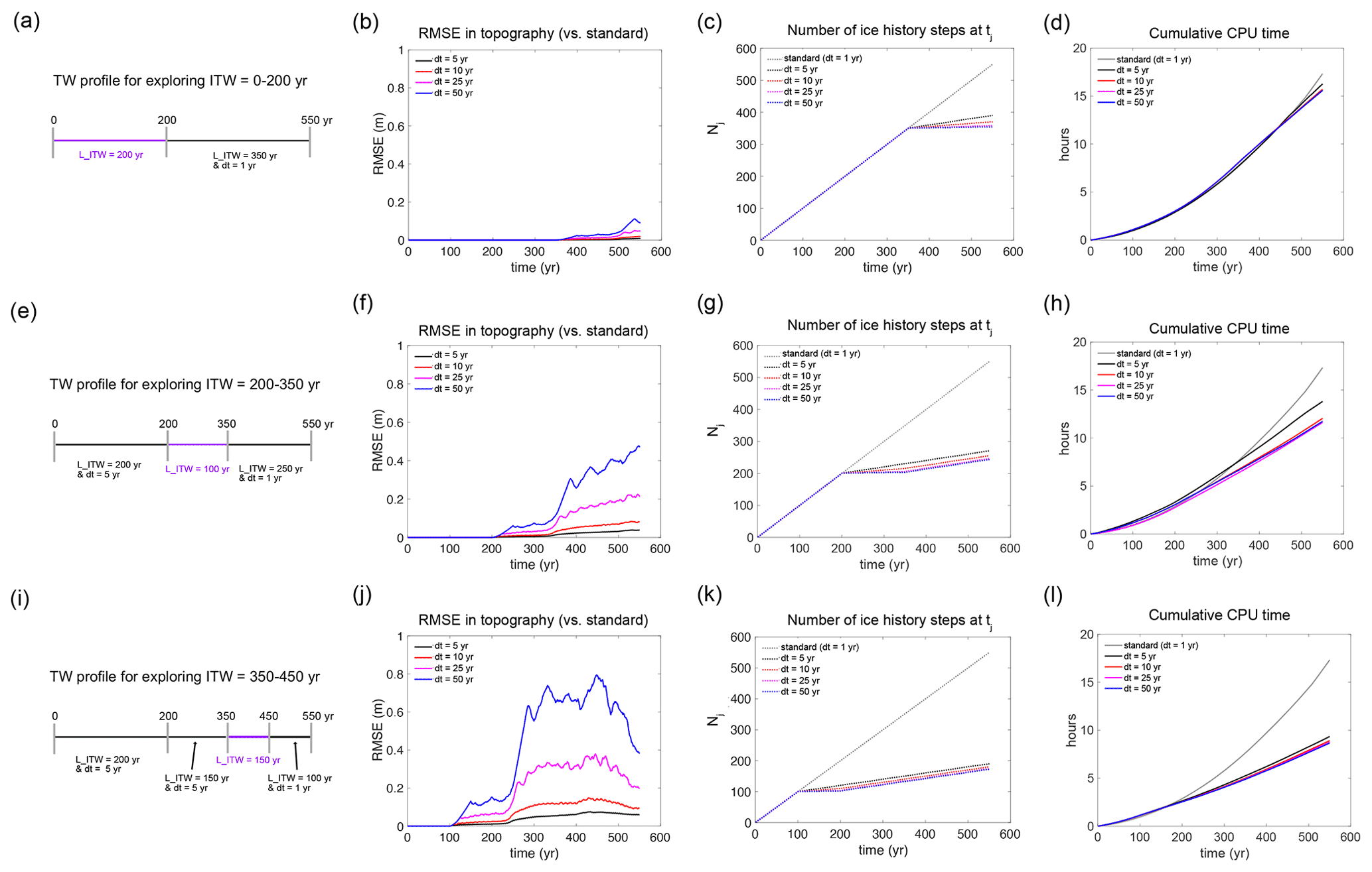
Figure 7 Time window profiles, RMSE in predicted topography, the number of loading events considered at t_j (N_j) and the total CPU times it has taken for the sea-level model to perform calculations at time step t_j in the 550-year-long future AIS-scenario simulations. Results from the simulations in which we explore the internal time windows that cover the periods between (a–d) 0–200 years, (e–j) 200–350 years and (i–l) 350–450 years. Note that the standard simulation for the AIS scenario assigns a uniform time-step size of 1 year throughout the simulation.

To test the performance of the time window derived in Fig. 7 in coupled ice-sheet–sea-level simulations, we perform a suite of coupled Antarctic-Ice-Sheet–sea-level simulations incorporating different coupling time intervals with the same climate forcing (RCP 8.5) scenario used in DeConto et al. (2021). Figure 9 shows smaller Antarctic ice volume and thickness for simulations with longer (uniform) coupling intervals such as dt=25 and 50 years. This is because a shorter coupling interval results in stronger ice-sheet stabilization. Geographically, the West Antarctic region that goes through the most intense retreat shows the largest differences in ice thickness that reach up to hundreds of meters (second and third column frames of Fig. 9). On the other hand, results from the coupled simulations that incorporate the time window algorithm show substantially smaller differences in ice volume and thickness compared to the benchmark simulation (fourth-column frames of Fig. 9). This is also shown in Fig. 10, which shows the cross section of ice thickness and topography along the red line shown in Fig. 6d. The differences in ice thickness and topography are only a few meters when we incorporate the time window profile derived earlier in this section.

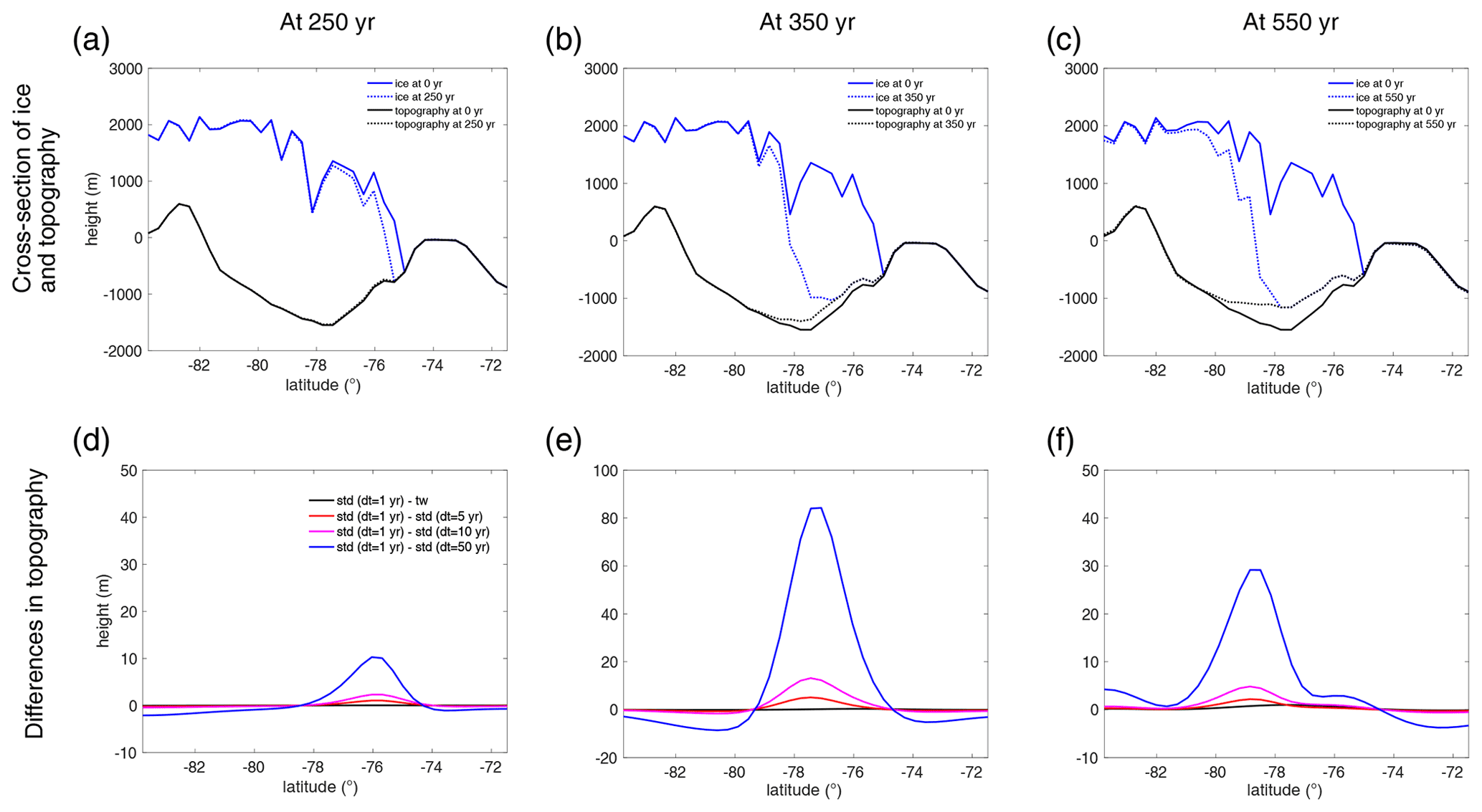
Figure 8 Elevations of the ice sheet and topography across the grounding line in the West Antarctic region (red line shown in Fig. 6g) and the sensitivity of predicted topography to temporal resolution in standard and time window simulations based on a stand-alone (uncoupled) sea-level model. (a–c) Ice surface (blue lines) and topography (black lines) predicted from the standard (std) simulation at (a) 250 years (dashed lines), (b) 350 years (dashed lines) and (c) 550 years (dashed lines) relative to the initial simulation time of 0 years (solid lines). The cross section of the grounding line is shown by a red line in Fig. 6d. (d–f) Differences in topography at (d) 250 years, (e) 350 years and (f) 550 years, between the benchmark simulation (dt=1 year) and the time window simulation (black lines) that incorporates dt=1 year for the most recent 100 years and dt=5 years for the rest of the 450 years of the simulation (i.e., black line in Fig. 7h), and between the benchmark simulation and standard simulation with dt=5 years (red lines), dt=10 years (magenta lines), and dt=50 years (blue lines). Note the change in the y axis in (e).

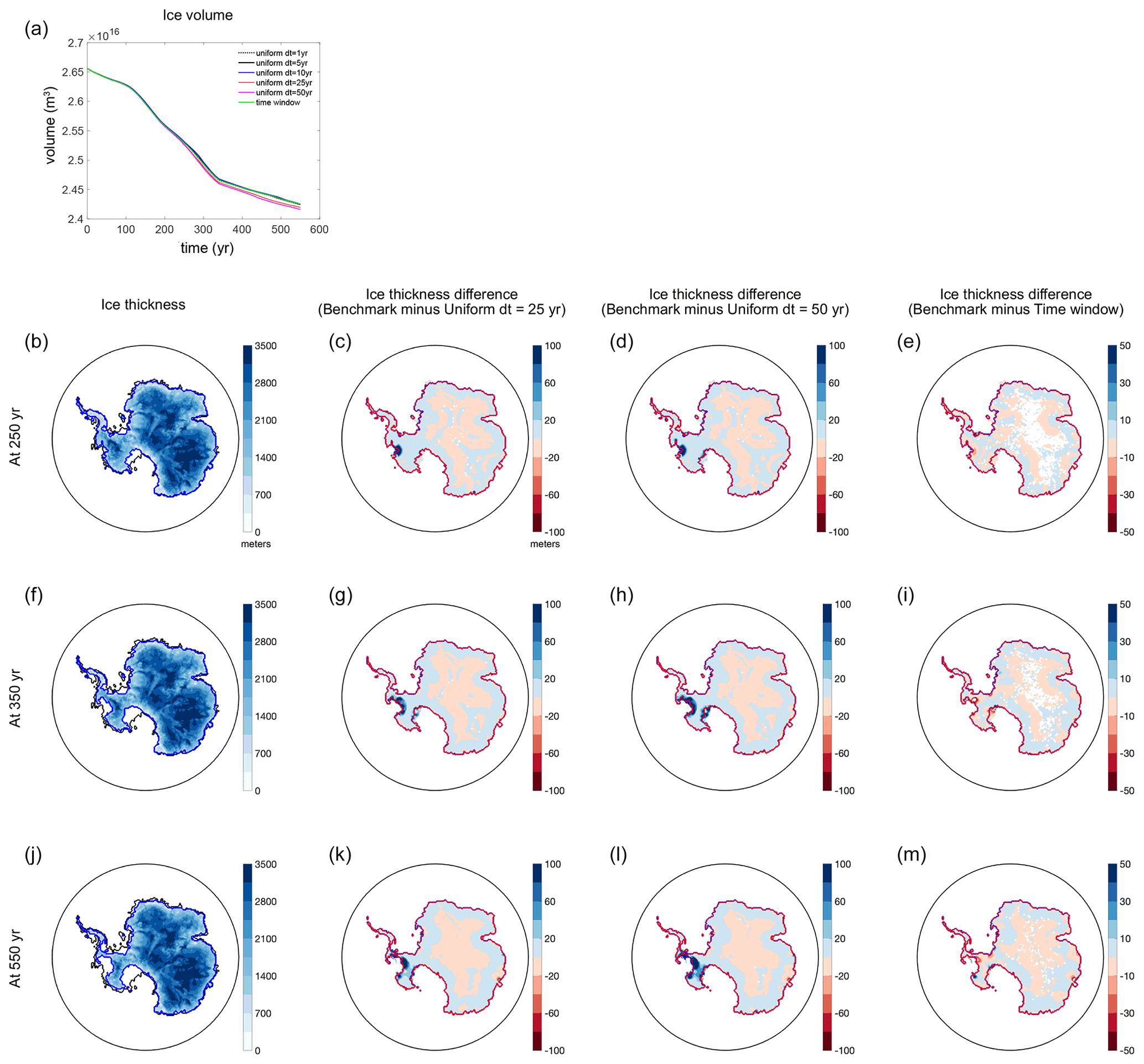
Figure 9 Changes in Antarctic Ice Sheet volume and thickness from coupled ice-sheet–sea-level simulations over 550 years adopting a RCP 8.5 scenario from DeConto et al. (2021). (a) AIS volume variations through 550 years from simulations that incorporate uniform (standard) coupling intervals of 1 (benchmark), 5, 10, 25 and 50 years and that incorporate the time window profile derived in Fig. 7. (First column) Ice thickness modelled in the benchmark simulation and differences in ice thickness between the benchmark and the standard simulations that incorporate coupling interval of (second column) 25 years and (third column) 50 years and that incorporates (fourth column) the time window profile. Each row shows results at a different simulation time at (b–e) 250 years, (f–i) 350 years and (j–m) 550 years. Note that the colour bars are saturated in the second and third column frames.

4 Discussion and conclusions

We have developed a new time window algorithm that assigns non-uniform temporal resolution to the input ice cover changes and restricts the linear increase in the number of ice history steps (or equivalently, the quadratic increase in computation time) in 1D pseudo-spectral sea-level modelling. Our algorithm allows coupled ice-sheet–sea-level models to capture short-term O(≤10² years) interactions between ice sheets, the solid Earth and sea level within simulations across a range of timescales. The algorithm improves computational feasibility while maintaining the precision of modelled topography and ice volume in stand-alone sea-level simulations and coupled ice-sheet–sea-level simulations.

In benchmarking the algorithm, we first tested the sensitivity of sea-level model outputs (i.e., predicted topography) to the temporal resolution adopted in idealized simulations (Fig. 2). Our results show that sea-level simulations with coarser temporal resolution do not accurately capture the timing and geometry of ice loading, which leads to an underestimation of topography changes if ice increments are assumed at the end of the time step. Our results also show stronger sensitivity to more recent loading (as suggested in earlier literature, e.g., Peltier, 1974), indicating that higher temporal resolution is required close to the current time step in a simulation. We then performed coupled ice-sheet–sea-level simulations through the last glacial cycle over the Northern Hemisphere with varying temporal resolution. Our results demonstrate that the underestimated magnitudes in predicted topography and infrequent topography updates in the coupled simulation with a lower temporal resolution lead to smaller and sometimes less-smooth ice volume fluctuations (Fig. 3a). Our results also identify that 0.2 kyr is the appropriate coupling time interval for glacial-cycle simulations, with 1D Earth structure typically adopted in global sea-level studies. When we utilize the time window algorithm and capture short-term, recent interactions while assigning coarser temporal resolution beyond the most recent 5 kyr during the simulation, the NHIS dynamics through the last glacial cycle are captured well while reducing the computation time by ∼ 26 %–31 % (Fig. 3b–d).

After benchmarking the time window algorithm, we explored suitable time window parameters that improve computational efficiency while maintaining the precision of model outputs for two different sea-level model applications: a simulation of global ice-sheet evolution through two glacial cycles (Figs. 4, 5) and a centennial-timescale future WAIS retreat scenario with an adopted Earth structure characteristic of the region with a thin lithosphere and low mantle viscosities (Figs. 6–10). The sample time window parameters we provide improve computational efficiency by ∼ 54 % and ∼ 50 % for each application, respectively, and the improvement would grow for longer simulations.

Overall, our results demonstrate the importance of incorporating higher temporal resolution in sea-level models in capturing short-term sea-level and ice-sheet responses during a period including and temporally close to ongoing surface loading changes. At the same time, a coarser temporal resolution can be used for past loading changes. This is expected based on normal mode theory where the solid Earth signals comprised of normal modes with shorter decay times associated with the loading changes would have already relaxed out after simulations have proceeded (Peltier, 1974).

Previously, de Boer et al. (2014) developed what they call a “moving time window” algorithm in their coupled ice-sheet–sea-level model, which they applied to global ice sheets over four glacial cycles (410 kyr). They utilized the characteristics of exponentially decaying viscous deformation and the linearity of 1D Maxwell viscoelastic rheology and interpolated “future” bedrock deformation associated with ongoing surface loading changes at the current time step for a predefined length of “memory” of the solid Earth (they set the memory length to be 80 kyr). Then, at every new time step, they calculated the total bedrock deformation associated with past loading changes by adding up the pre-interpolated bedrock deformation in the previous time steps. This algorithm allows them to perform global coupled simulations over multiple glacial cycles.

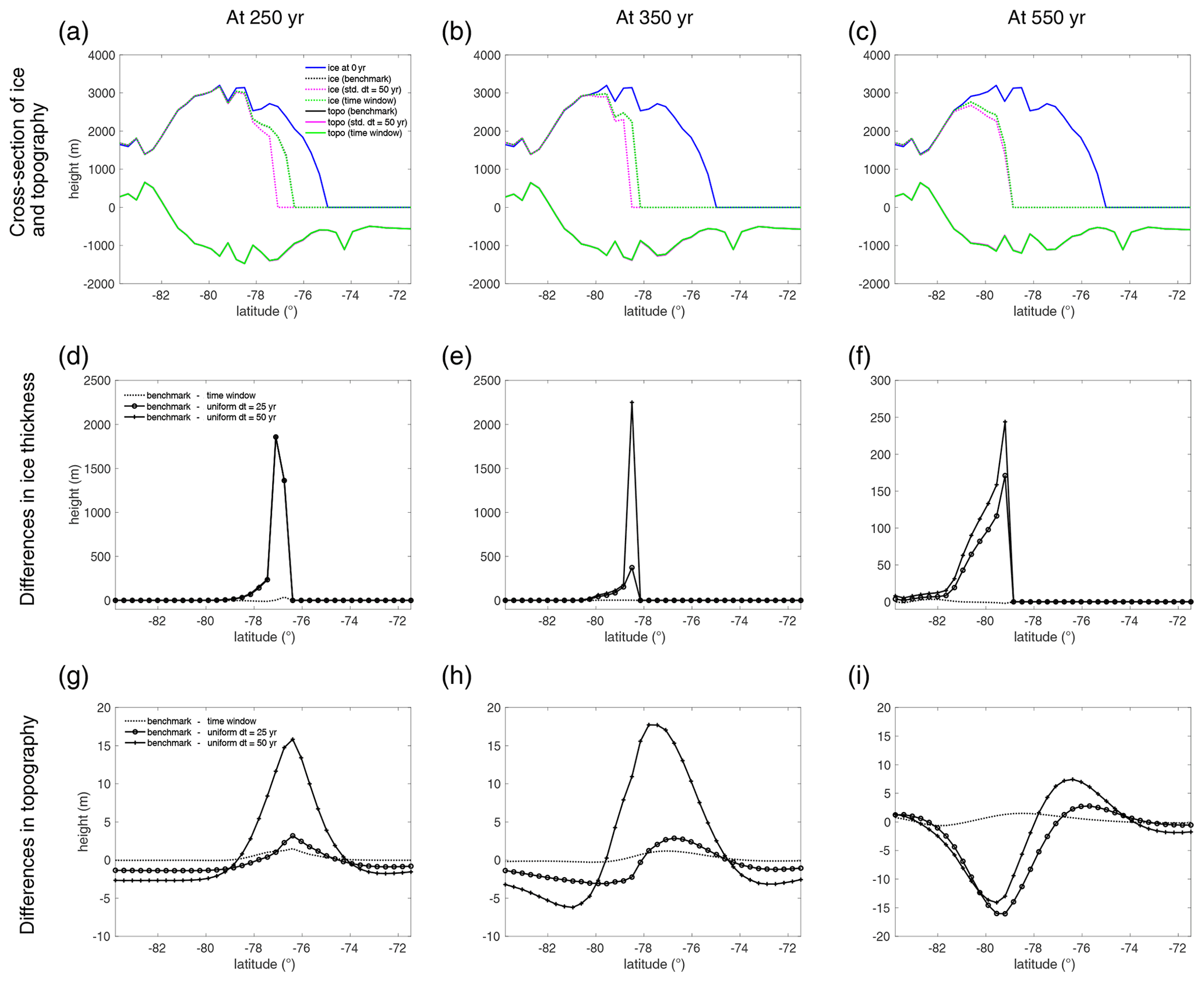
Figure 10 Predicted elevations of ice sheet and topography across the grounding line in the West Antarctic region (red line shown in Fig. 6g) in coupled ice-sheet–sea-level simulations with and without the time window algorithm and the differences in the predicted ice thickness and topography. (a–c) Cross section of ice thickness and topography at (a) 250 years, (b) 350 years and (c) 550 years. Blue lines indicate ice profile at the beginning of the simulation. Black lines show results from the benchmark standard coupled simulation that incorporates temporal resolution of 1 year, magenta lines show results from the standard simulation with dt=50 years, and green lines show results from the simulation that incorporates the time window profile derived in Fig. 7. Dashed lines show ice thickness, and solid lines show topography. (d–f) Differences in ice thickness at (d) 250 years, (e) 350 years and (f) 550 years between the benchmark coupled simulation and the simulation incorporating the time window profile (dotted lines) and standard simulations with dt=25 years (circled lines) and dt=50 years (crossed lines). (g–i) Same as (d–f) but showing differences in topography.

Rather than pre-calculating the future response as in de Boer et al. (2014), our time window recalls past ice loading changes in changing levels of detail as the simulation proceeds, allowing us to keep the high-frequency coupling interval of annual–centennial timescale in coupled ice-sheet–sea-level simulations. In addition, our sea-level model with the time window is capable of iterative topography correction (as described in Kendall et al., 2005, and applied in a coupled context in Gomez et al., 2013) that allows for modelled present-day topography to converge to the observed present-day topography even when the model is coupled to a dynamic ice-sheet model. Considering that the topography correction is required in paleo-glacial-cycle simulations in which initial topography is unknown and that the correction typically takes 2–3 additional iterations of the whole glacial-cycle simulation to achieve the convergence, the computation time saved by the time window algorithm becomes greater for paleo-simulations.

As for the coupling time interval, our results suggest that it should be at least 0.2 kyr for glacial-cycle simulations, which is shorter than 1 kyr suggested by de Boer et al. (2014) who claimed that 1 kyr is a sufficiently short coupling interval for their glacial-cycle simulation. Our results indicate that a coupling time interval of 1 kyr causes a significant difference of up to ∼ 11.6 m of difference in the predicted sea-level equivalent Northern Hemisphere ice-sheet volume compared to the simulation that incorporates the coupling time interval of 0.2 kyr. This difference in the conclusion of ours and that of de Boer et al. (2014) may be attributed to different spatial resolution of the sea-level model incorporated in each study: our sea-level model uses three-times finer spatial resolution than theirs, which uses spherical harmonics expansion up to degree and order 128. Furthermore, the sensitivity of ice dynamics to bedrock elevation changes may also be ice-sheet-model-dependent (e.g., Larour et al., 2019; Wan et al., 2022).

In general, adopting a shorter coupling time comes at the expense of computational cost, and the choice of appropriate coupling time for a given application will depend on both the resolution and timescale of ice-sheet variations, as well as the adopted Earth structure model. In this context, a shorter coupling time is required for fast-evolving ice sheets on the solid Earth with low mantle viscosity (like the WAIS) since the relaxation time of the solid Earth is faster (slower) for Earth's mantle with lower (higher) viscosity. West Antarctica is underlain by low mantle viscosity O(10¹⁸⁻¹⁹ Pa s) (Barletta et al., 2018; Lloyd et al., 2020) and will respond viscously in a faster, more localized manner to surface loading changes, and this has the potential to have a significant impact on future evolution of marine ice in the region. Furthermore, recent work by Larour et al. (2019) suggests that high spatial resolution and short time stepping may be required to capture the elastic component of deformation in this region. These studies suggest that an annual- to decadal-scale coupling time is likely needed to capture the short-term interactions in a coupled model that may play a significant role in the stability of marine-based WAIS. In Sect. 3.3.2, we performed a benchmark sea-level simulation with future WAIS evolution at 1-year temporal resolution. We then introduced a set of time window parameters that allow us to keep a coupling interval of 1 year while improving the total CPU time by 50 % (Fig. 7) and maintaining the precision in predicted topography (Fig. 8) and ice-sheet dynamics (Figs. 9, 10) in West Antarctica. We have adopted the shortest temporal resolution suggested in the literature to date (Larour et al., 2019) for the benchmark sea-level simulation in our analysis, but given the complexity of Earth's structure and ice dynamics in this region, further exploration with a coupled ice-sheet–sea-level model will be needed to rigorously assess the coupling time interval needed to simulate ice-sheet evolution in marine sectors of the AIS.

Overall, we have presented a new time window algorithm that can be applied to global 1D forward sea-level models based on normal mode theory (Peltier, 1974). We also have provided sample time window parameters for applications to global glacial-cycle ice-sheet evolution and rapid marine ice-sheet retreat in a region with weaker Earth structure. A next step in algorithm development could be to implement an adoptive time window scheme in the sea-level model such that the time window profiles self-adjust to ice-sheet variability within the simulation. Meanwhile, we have shown that our time window algorithm achieves the goal of overcoming computational challenges introduced in coupled ice-sheet–sea-level modelling while broadly capturing ice-sheet–sea-level feedbacks, especially considering the range of other sources of uncertainties in the ice-sheet and sea-level model components. In addition to the applications we have shown in this study, the time window algorithm has the potential to unlock opportunities to tackle a range of questions using coupled ice-sheet–sea-level modelling, such as evaluating shorelines during and since the warm mid-Pliocene (3 Ma; Raymo et al., 2011; Pollard et al., 2018), investigating the effects of short-term interactions between ice sheets, sea level and the solid Earth on the dynamics of the marine-based portion of Eurasian Ice Sheet during the last deglaciation phase (e.g., Petrini et al., 2020) and the associated impact on abrupt or episodic global sea-level events such as Meltwater Pulse 1A; e.g., Harrison et al., 2019), and understanding the dynamics of ice sheets during past warm interglacial periods (e.g., Clark et al., 2020). Finally, the improved computational feasibility with the time window could allow for ensemble simulations of coupled ice-sheet–sea-level dynamics for the future under different warming scenarios, which will provide useful insight into sea-level projections.