the Creative Commons Attribution 4.0 License.
the Creative Commons Attribution 4.0 License.
 | 07 Jan 2022
ISWFoam: a numerical model for internal solitary wave simulation in continuously stratified fluids
Jingyuan Li
Tongqing Chen
A numerical model, ISWFoam, for simulating internal solitary waves (ISWs) in continuously stratified, incompressible, viscous fluids is developed based on a fully three-dimensional (3D) Navier–Stokes equation using the open-source code OpenFOAM®. This model combines the density transport equation with the Reynolds-averaged Navier–Stokes equation with the Coriolis force, and the model discrete equation adopts the finite-volume method. The k–ω SST turbulence model has also been modified according to the variable density field. ISWFoam provides two initial wave generation methods to generate an ISW in continuously stratified fluids, including solving the weakly nonlinear models of the extended Korteweg–de Vries (eKdV) equation and the fully nonlinear models of the Dubreil–Jacotin–Long (DJL) equation. Grid independence tests for ISWFoam are performed, and considering the accuracy and computing efficiency, the appropriate grid size of the ISW simulation is recommended to be 1150th of the characteristic length and 125th of the ISW amplitude. Model verifications are conducted through comparisons between the simulated and experimental data for ISW propagation examples over a flat bottom section, including laboratory scale and actual ocean scale, a submerged triangular ridge, a Gaussian ridge, and slope. The laboratory test results, including the ISW profile, wave breaking location, ISW arrival time, and the spatial and temporal changes in the mixture region, are well reproduced by ISWFoam. The ISWFoam model with unstructured grids and local mesh refinement can effectively simulate the evolution of ISWs, the ISW breaking phenomenon, waveform inversion of ISWs, and the interaction between ISWs and complex topography.
- Article
(13131 KB) - Full-text XML
- Companion paper
- BibTeX
- EndNote


Internal solitary waves (ISWs) are commonly observed in oceans, particularly in continental shelf regions, due to strong tidal current flows over large topographic features (Huthnance, 1981), such as in the northern South China Sea (Alford et al., 2010, 2015; Cai et al., 2012). ISWs play an important role in both conveying nutrients from the deep ocean to shallower layers and promoting biological growth (Sandstrom et al., 1984). Additionally, ISWs are a potential threat to the ocean structures of resource exploration, exploitation and submarine navigation vehicles (Alford et al., 2010; Osborne and Burch, 1980). A considerable number of studies, which include field measurements, remote sensing, experiments, theoretical analysis and numerical simulations, have been carried out due to the significance of ISWs (Vlasenko et al., 2005; Apel et al., 2006; Alford et al., 2011; Guo et al., 2014).
For numerically simulated ISWs, many models have been adopted, including the Euler equation, the inviscid or viscid incompressible Boussinesq model, the hydrostatic model, the non-hydrostatic model, and the VOF-based two-phase flow model. Among these models, the representative hydrostatic models include the Naval Research Laboratory Ocean Nowcast/Forecast System (ONFS) (Ko et al., 2008), the Regional Hallberg Isopycnal Tide Mode (RHIMT) (Hallberg and Rhines, 1996; Hallberg, 1997) and the Ostrovsky–Hunter model. The representative non-hydrostatic models include the Bergen Ocean Model (BOM), the nonhydrostatic Regional Ocean Modeling System model (ROMS), the Stanford Unstructured Nonhydrostatic Terrain-following Adaptive Navier–Stokes Simulator (SUNTANS) and the Massachusetts Institute of Technology general circulation model (MITgcm). For example, Zhang et al. (2012) established a variable-water-depth internal-wave numerical model in a continuously stratified fluid system based on the Euler equation. Xu and Stastna (2020) used the viscid incompressible Boussinesq model to study cross-boundary-layer transport (Boegman and Stastna, 2019) by the fissioning process of shoaling ISWs. Lamb (1994) established a non-hydrostatic model, using a second-order projection method developed by Bell and Marcus (1992), which is used for internal-wave research including boundary-layer instability (Aghsaee et al., 2012), reflection (Lamb and Nguyen, 2009 ), and the interaction of the tides with the topography (Lamb, 2007; Aghsaee et al., 2010). Diamessis (2005) developed a spectral multidomain penalty method model and correctly reproduced the characteristic vorticity and internal-wave structure. Subich et al. (2013) developed a spectral collocation method for the solution of the Navier–Stokes equations under the Boussinesq approximation and simulated the internal wave in continuously stratified fluid. Smedstad et al. (2003) employed the ONFS model to establish a global ocean real-time forecasting system with an operational eddy resolution of ∘, which effectively tracks ocean eddies, ocean currents and ocean fronts. Simmons et al. (2004) employed the RHIMT model to carry out a global numerical simulation of tidal currents and analysed the whole process of the conversion rate of barotropic waves into baroclinic waves. Thiem (2011) used the Bergen Ocean Model to explore the bottom boundary-layer flow caused by waves beneath a propagating ISW in a two-fluid system. Li and Farmer (2011) employed the Ostrovsky–Hunter model to study the nonlinear evolution of a monochromatic internal wave. Buijsman et al. (2010) employed a ROMS model to study the asymmetry in solitons to the east and west of the Luzon Strait. Zhang et al. (2011) used the nonhydrostatic SUNTANS model (Fringer et al., 2006) to study the dynamics of A-wave and B-wave formation. Rayson et al. (2018) used the modified SUNTANS model to study the internal waves around Scott Reef and provided the generation process of internal lee waves. Vlasenko et al. (2010) employed the MITgcm model to investigate the baroclinic tidal energy conversion in the area west of the Luzon Strait.
In summary, for continuously stratified fluids in complex ocean environments, numerical simulation has become a leading method for ISW investigations. However, there are presently few versatile numerical models with shared code that can accurately simulate the ISW flow around complex topography and submarine navigation vehicles in continuously stratified fluids. Therefore, the main objective of this paper is to develop a solver, referred to as ISWFoam with a modified k–ω SST model that considers the variable density field, which simulates the ISW in continuously stratified, incompressible and viscous fluids using the finite-volume method with unstructured grids based on a fully three-dimensional (3D) Navier–Stokes equation using the OpenFOAM® library.
Notably, the open-source field operation and manipulation code OpenFOAM, as an object-oriented C open-source library that can be used to build a variety of solvers for computational fluid problems based on the finite-volume method, is becoming increasingly popular in the computational fluid research community. At present, the official version of OpenFOAM does not have a solver or boundary conditions for solving the ISW in continuously stratified fluids. Although some researchers simulate ISWs by modifying the OpenFOAM code, most of these studies are based on a two-fluid system without considering continuous stratification in density, such as Meng and Zhang (2016) and Li et al. (2017). Though recent work by Ding et al. (2020) and Li et al. (2021) considered continuous stratification in density, their wave generation theories do not consider continuous stratification in density. To extensively use the numerical model of ISWs as a tool in the future, we will develop ISWFoam to simulate the ISW in continuously stratified, incompressible and viscous fluids based on the OpenFOAM library. The turbulence model will consider the variable density field. In addition, ISWFoam will provide two initial methods to generate an ISW in continuously stratified fluids, including solving the weakly nonlinear models of the extended Korteweg–de Vries (eKdV) equation and the fully nonlinear models of the Dubreil–Jacotin–Long (DJL) equation. This approach renders the numerical model suitable for the simulation of ISW flows in complex geometries and topographies. It is worth noting that ISWFoam does not consider the generation process of ISWs but focuses on the propagation and evolution of ISWs that have already been generated, and the interaction between ISWs and complex structures and topography on field scales.
The outline of the paper is described as follows. First, in Sect. 2, the governing equations for a continuously stratified fluid are presented, and discrete forms of these equations are derived. Then, grid independence tests of the developed ISWFoam model are described in Sect. 3. Subsequently, in Sect. 4, a series of test cases are presented to verify the model. Simulation examples at the field scale are shown in Sect. 5. Finally, the conclusions are drawn in Sect. 6.
2.1 Governing equations
We present an ISW numerical model by solving the motion of a three-dimensional, viscous, incompressible fluid with the Boussinesq approximation and rigid lid hypothesis. The governing equations of the model are
where U = (ui, uj, uk) is the velocity vector, t is time, ∇ is the gradient operator, Q is the source term, ρ0 is the reference density, ρ is the density field, p_rgh is a modified pressure field, g is the gravitational acceleration vector and X is the position vector. vEff is the effective kinematic viscosity defined as , where μEff is the effective dynamic viscosity including the molecular viscosity (μl) and turbulent viscosity (μt). k is the diffusion coefficient, and its value is the same as the effective dynamic viscosity(μEff). Ω is the Coriolis parameter, which is twice the speed of rotation around the vertical unit vector e3= (0, 0, 1). ISWFoam uses a modified pressure p_rgh instead of a total pressure p, and their relationship is given by
The upper boundary (z=H, with H the depth of computation domain) is treated as a rigid lid, and the kinematic boundary conditions for this boundary are given by
To close the above equations, the turbulence model needs to be employed. The two-equation k–ε model is widely used as an effective turbulence model, but it cannot capture the proper behaviour of turbulent boundary layers up to separation due to adverse pressure gradients (Wilcox, 1993). For the above boundary-layer separation problem, Bardina et al. (1997) and Menter et al. (2003) suggested the use of the k–ω shear stress transport (SST) model to obtain substantially more accurate results. Therefore, the turbulence model used in this paper is the k–ω SST model. Note that in OpenFOAM, the incompressible version for turbulence models does not consider the variable density field, and instead, it treats the density as a constant, such as in the k–ω SST model:
where k is the turbulent kinetic energy, ω is the specific dissipation rate; Pk is the production term of k; ; is related to the production term of turbulence kinetic energy Pk in the k equation; vt is the turbulent kinematic viscosity; St is the mean rate of the flow strain; St=0.5(∇U+∇UT); the model constants are assigned the values , a1=0.31, c1=10 and Cμ=0.09; F1 and F2 are blending functions; and the value of σk, σω, Cγ and Cβ are blended using the equation in which Ô1 and Ô2 are given in Table 1.

Considering the variable density field during the solution process, it is necessary to consider the change in the density field in the turbulence model. Therefore, we modify the turbulence model to consider the change in density, and finally a modified k–ω SST model that considers the change in density is used to close the equation:
2.2 Numerical discretisation
The governing equations are numerically discretised using the finite-volume method based on the C open-source library of OpenFOAM. The finite-volume method requires that Eqs. (2) and (3) are satisfied over the control volume VP around point P in integral form:
where Δt is the time step.
The momentum equation in ISWFoam is solved by constructing a predicted velocity field and then using the pressure implicit with splitting of operators (PISO) algorithm (Issa, 1986) to modify it. n is defined to represent the current moment. The PISO iteration process is marked as m; when m is equal to zero, it represents the current time (tn).
First, only the temporal, convection and diffusion terms appear in the discrete version of the equation momentum, and the other terms are ignored. After this operation, we obtain an explicit expression for the predicted velocity field , namely,
where P represents the centre of the grid cell, is the volume flux at the initial time n and Sf is the face vector.
The solution process requires the velocity on the surface f. Assuming the variation in between the centre P of the grid and the centre N of the adjacent grid, the face values are calculated using a mixture method (blended differencing) of the central scheme (central differencing) and the upwind scheme (upwind differencing) as follows (Jasak, 1996):
where
where N represents the centre of the adjacent grid cells, and is volume flux. The limiter λU can be selected from several alternatives (OpenFOAM, 2019), including linear, QUICK, van Leer, etc. In the following derivation process, the van Leer scheme was used to calculate the velocity of the face centre
where ψ(ϕf) is a step function defined by
Inserting Eq. (15) into Eq. (13) yields
After some manipulation, the quantities AP and AN are given as
Including the effect of gravity and the Coriolis force in Eq. (17),
Notably, that when m is equal to zero, it represents the initial moment n, and the value of the initial moment is known. Therefore, we obtain the predicted velocity field in the first iteration. We define the surface gradient operator , and the type of gradient operator acting on U is , which represents the distance from the centre of the grid N to P. Similarly, the surface gradient operator acting on scalar γ is . The associated flux ( is achieved by executing an inner product with a surface vector (Sf) on the left and right parts of Eq. (20), giving
Equation (21) completed the flux calculation without considering the influence of the pressure term. The pressure contribution in terms of a flux can be expressed as
Then, Eq. (22) is added to Eq. (21) to yield
Combined with Eq. (21), Eq. (23) is simplified and rewritten as
Using conservation of mass, we solve the pressure field , which results in
The preconditioned conjugate gradient method is used to solve the linear system constructed by Eq. (25) (OpenFOAM, 2019). After is obtained using Eq. (25), we calculate the volume flux using Eq. (24) for each face. The cell-centred velocity fields are calculated by reconstructing the face velocity flux using the following expression (Deshpande, 2012):
Equation (26) completes the velocity field calculation of the first iteration step in the PISO algorithm. By converting the identifier m to m+1, the next PISO iteration is completed and updates the velocity in Eq. (17) with the velocity calculated from Eq. (26), thereby updating p_rgh, ϕf and U. This procedure is performed M times to guarantee that the results of the velocity and pressure together conform to the continuity and momentum equations. Considering that PISO iteration levels require more than 1, but typically not more than 4 (OpenFOAM, 2019), we specify that the number of PISO iteration levels is 3 in the computations presented in this paper. After completing the three iterations, the converged values are considered the result of the next time step (n+1), namely,
We discretise the convection–diffusion equation of density (Eq. 12) to obtain
At the end of the iteration procedure, we bring the results of the volume flux into Eq. (28) to calculate the density field at the next time (, thereby updating the density field for the next step calculation ().
2.3 Initialised field of ISW generation
ISW generation methods mainly include the gravity collapse mechanism, double push-pedal method (Fu et al., 2008), velocity-inlet method (Gao et al., 2012), mass source method (Wang et al., 2018), initialisation method, and methods addressing the interaction between tidal current and topography. For example, Hsieh et al. (2014) investigated the flow evolution of a depression ISW generated by the gravity collapse mechanism. Cheng et al. (2020) studied the interaction between ISWs and a cylinder using the gravity collapse mechanism. The initialisation method involves solving the internal solitary wave theory at the initial moment, such as the Korteweg–de Vries (KdV) equation (Grimshaw et al., 2010), the modified KdV (mKdV) equation, the extended KdV (eKdV) equation, the forced KdV equation, the Ostrovsky equation (Li and Farmer, 2011), the Miyata–Choi–Camassa (MCC) model (Miyata, 1985, 1988; Choi and Camassa, 1999) and the Dubreil–Jacotin–Long (DJL) equation (Long, 1953; Turkington, 1991; Brown and Christie, 1998; Dunphy et al., 2011), to obtain the wave surface and velocity field. The method of an interacting between tidal current and terrain that stimulates ISWs is adopted by many scholars, such as Farmer and Smith (1980), Lamb et al. (1994), and Shaw et al. (2009).
In this paper, the method of initialising the field is selected to generate the ISWs. To increase the application range of the ISWFoam model, two initialisation methods are provided, including solving the weakly nonlinear models of the eKdV equation (Helfrich and Melville, 2006) and the fully nonlinear models of the DJL equation for continuously stratified fluids (Turkington, 1991; Dunphy et al., 2011). The Dubreil–Jacotin–Long (DJL) equation is expressed as
where η is the isopycnal displacement, H is the water depth, c is the propagation speed, N is the definition of the buoyancy frequency, and z is the vertical position.
where ρ0(z) is the reference density, and g is the gravitational acceleration.
By solving the above DJL equation we can obtain η and c, and then through the relationship ψ=ηc, where ψ is the stream function, we can obtain the wave-induced velocity field. We use the DJLES open-source package provided by Dunphy et al. (2011) to solve the DJL equations. Then we input the initial field calculated by DJLES into OpenFOAM to obtain the initial field required for OpenFOAM numerical simulation.
Another theory of ISWFoam model wave generation involves the weakly nonlinear models of the eKdV equation. Using the first-order stream function for the DJL equation, we can obtain the well-known KdV equation and further obtain the eKdV equation. For the specific derivation, please refer to the paper by Lamb and Yan (1996). The eKdV equation (Helfrich and Melville, 2006) is
where ζ is the isopycnal vertical displacement; c0 is the linear phase speed; the coefficients c1, c2 and c3 are functions of the steady background stratification and shear through the linear eigenmode (vertical structure function) of interest (Helfrich and Melville, 2006); h1 and h2 are the mean upper and lower layer depths, respectively; and ρ1 and ρ1 are the fluid densities of the upper and lower layers, respectively. The theoretical solution of Eq. (31) above is
where a is the ISW amplitude, λeKdV is the wavelength, ceKdV is the wave speed, B is an auxiliary parameter, and u1 and u2 are the speeds of the upper and lower layers of the fluid, respectively. The waveform and velocity field of the ISWs are solved at the initial moment by the developed function and then assigned to the calculation domain.
The vertical profile of the initial density is given by a hyperbolic tangent function profile (Aghsaee et al., 2010):
where z is the vertical position; ρ1 and ρ2 are the fluid densities of the upper and lower layers, respectively; zpyc is the location of the centre of the pycnocline; and dpyc is the thickness of the pycnocline. In this paper, unless otherwise specified, the form of the density profile adopts Eq. (41). The internal solitary wave surface is obtained by calculating the gradient of the density field, and the absolute value of the maximum value of the gradient represents the vertical position of the wave surface. Notably, the density profile of the actual ocean is not always hyperbolic, so our model provides a function for users to modify the density profile according to the actual situation.
2.3.1 Comparison between the DJL equation and the eKdV equation
To compare the DJL equation and the eKdV equation, we set up a numerical simulation, which includes a tank that is 15 m long, 1 m wide and has a water depth of 0.5 m. The depths of the upper (h1) and lower (h2) layers are 0.1 and 0.4 m, respectively; the densities of the upper and lower layers are 1022 and 1028 kg m−3, respectively; the location of the centre of the pycnocline (zpyc) is 0.4 m; the pycnocline thickness (dpyc) is 0.04 m vertically; the initial ISW amplitude (a) is 0.065 m; and the location of the centre of ISW is 12.5 m. The ISWs propagate from right to left. The measuring point P is set at a position 10 m away from the initial ISW. The grid is uniform in the x direction, y direction and z direction, and the sizes are m, m and m, respectively. Slip boundary conditions are applied to the bottom and both sides, while cyclic boundary conditions are assigned to the inlet and outlet boundaries. The top boundary is a rigid lid. The boundary conditions related to the density field are no-flux boundary conditions.

Figure 1Comparison chart of the horizontal velocity component field: DJL equation (left) and eKdV equation (right).
Figure 1 shows the comparison of the horizontal velocity component field when the DJL equation and the eKdV equation are used to generate ISWs. At the initial moment, the ISW generated by the eKdV equation is not as smooth as the ISW generated by the DJL equation, and the horizontal velocity at the interface area is discontinuous as shown in Fig. 1a and b. With the propagation of ISWs, the ISWs generated by the DJL equation are always smooth at the interface area, and the velocity field is always continuous as shown in Fig. 1a, c, e and g. Correspondingly, the ISW generated by the eKdV equation gradually produces a gradient in the vertical direction of the horizontal velocity in the interface area; thus, the interface area becomes smooth, and the velocity becomes continuous. Fig. 1d shows this evolution process, which is basically completed in 5 s as shown in Fig. 1f. At 50 s, the difference between the horizontal velocity fields of the two equations is very small as shown in Fig. 1g and h.
Figure 2 shows the comparison of the vertical velocity component field when the DJL equation and the eKdV equation are used to generate ISWs. Since the theoretical solution of the eKdV equation only obtain the average horizontal velocity of the upper and lower layers of the fluid, there is no vertical velocity at the initial moment, as shown in Fig. 2b. With the propagation of ISWs, the vertical velocity field will gradually be generated and finally stabilised, and the stable time occurs at 5 s as shown in Fig. 2b, d, f and h. At 50 s, the difference between the vertical velocity fields of the two equations is very small as shown in Fig. 2g and h.
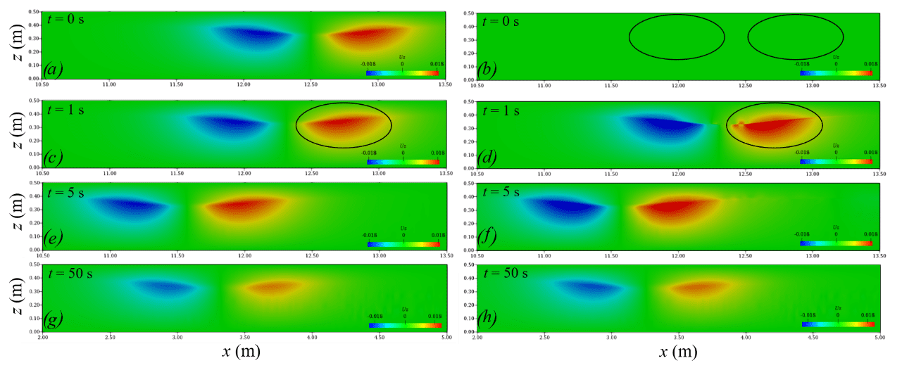
Figure 2Comparison chart of the vertical velocity component field: DJL equation (left) and eKdV equation (right).
The ISW propagates for 10 m, and the amplitudes of the ISWs generated by the DJL equation and the eKdV equation are reduced by 9.88 % and 17.96 %, respectively, as shown in Fig. 3. Overall, the reduction in energy leads to the attenuation of the amplitude of the ISW, which in turn reduces the wave speed. Except for the difference in initial fields, the grid sizes, time step, turbulence model and other features are the same. Therefore, the initial stage of ISWs generated by the eKdV equation leads to excessive energy loss compared with those generated by the DJL equation. From the above analysis of the velocity field, we know that the method of initialising the field with the eKdV equation requires a period of movement before the jump of the velocity field develops into a field with continuous changes in velocity. In addition, the DJL equation, as a fully nonlinear model, can better reflect its superiority for internal waves with strong nonlinearity. Therefore, the wave generation of the subsequent numerical cases in this paper adopts the method of initialising the field with the DJL equation.
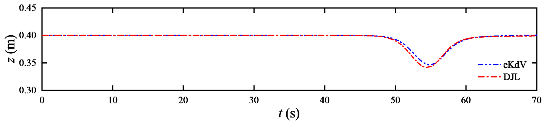
Figure 3Time series of the interface displacement. The probe was 10 m away from the initial ISW.
These grid independence tests were performed in the horizontal and vertical directions by applying meshes of different sizes. The sizes of the mesh determined in this paper are calculated based on the amplitude of the ISW and a characteristic length determined through the integration of the wave profile (Michallet and Ivey, 1999):
where ζ is the isopycnal vertical displacement and a is the ISW amplitude.
To determine the appropriate mesh size, the propagation of ISWs on flat bottoms is calculated, and the numerical results are compared with the DJL theoretical solution. We set up a numerical simulation, which includes a tank that is 50 m long, 0.5 m wide and has a water depth of 0.5 m. The depths of the upper (h1) and lower (h2) layers are 0.1 m and 0.4 m, respectively; the densities of the upper and lower layers are 1000 kg m−3 and 1030 kg m−3, respectively; the location of the centre of the pycnocline (zpyc) is 0.4 m; the pycnocline thickness (dpyc) is 0.05 m vertically; and the ISW amplitude a is 0.065 m. The measuring point P is set at a position 10L away from the initial ISW. The sponge layer on both sides, whose length is the double wave characteristic length, has been checked to properly dissipate the reflected wave. Slip boundary conditions are applied to the bottom and both sides, while cyclic boundary conditions are assigned to the inlet and outlet boundaries. The top boundary is a rigid lid. The boundary conditions related to the density field are no-flux boundary conditions.
3.1 Grid independence in the horizontal direction
First, we analyse the grid independence in the horizontal direction, with a constant cell height of m . Figure 4 shows the results of the comparison of the waveform and decay rate in the horizontal direction at probe P1 with the ISWFoam using a wide range of grid configurations. The results show a negligible difference in the waveform when the mesh size is less than 40, so it is difficult to accurately analyse the grid independence just by the waveform. A traditional decay rate parameter is adopted, namely δ=(aprobe – , where ainitial is the ISW amplitude value at the initial moment, and aprobe is the ISW amplitude value of the probe 10L away from the initial ISW. Figure 4b shows the relationship between the decay rate of the ISW amplitude and the grid quantity per unit length for different mesh sizes. As shown in Fig. 4b, the decay rate of the ISW amplitude tends to be smooth as the grid number per unit length increases to 160 (150), and then the increase in the grid quantity has a relatively small effect on the decay rate. Therefore, for ISWFoam developed in this paper, we suggest that the dimensions of the horizontal grid are 150.
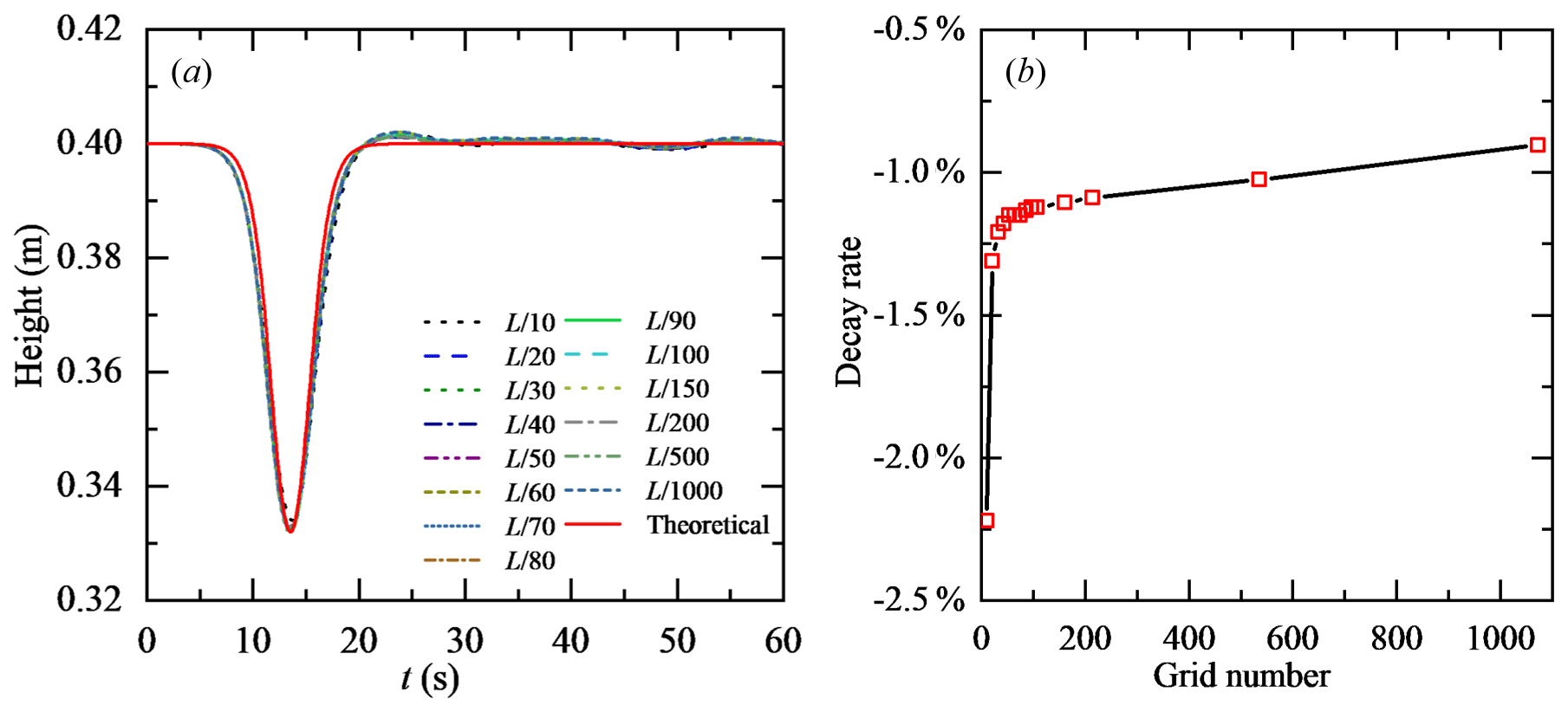
Figure 4Grid independence in the horizontal direction at probe P1: (a) comparison of waveform and (b) decay rate.
3.2 Grid independence in the vertical direction
Second, we analyse the grid independence in the vertical direction, with a constant cell width of 150 m. Figure 5 shows the results of a comparison of the waveform and decay rate of the ISW amplitude in the vertical direction at probe P1 with the ISWFoam using a wide range of grid configurations. The results also show a negligible difference in the waveform when the mesh size is less than 10, so it is difficult to accurately analyse the grid independence just by the waveform. As shown in Fig. 5b, the decay rate of the ISW amplitude decreases as the grid quantity increases in a wave height range before the numerical oscillation occurs. Here, we assume that the grid size with the decay rate of the ISW amplitude less than 1 % is the appropriate vertical grid size; namely, the vertical grid size is 25 m. Therefore, for ISWFoam developed in this paper, we suggest that the dimensions of the vertical grid be 25.
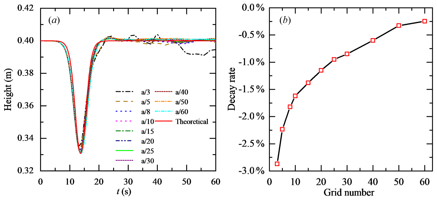
Figure 5Grid independence analysis in the vertical direction at probe P1: (a) comparison of waveform and (b) decay rate.
To verify the numerical model of the ISWs, the propagation of ISWs on a flat bottom section, submerged triangular ridge and slopes is calculated, and the numerical results are compared with the corresponding experimental results. To verify the correctness of Coriolis code implantation and reflect the role of local mesh refinement, the propagation of ISWs on a flat bottom section of actual ocean scale and a Gaussian ridge is calculated.
4.1 ISW propagating on a flat bottom section
4.1.1 Experimental data used
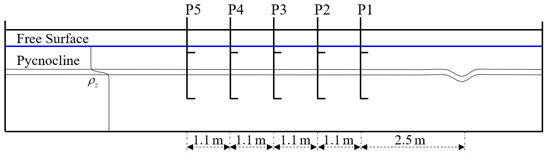
In this section, ISWFoam is verified by employing ISWs propagating on a flat bottom section with Case Flat_4 in the continuously stratified laboratory experiment described in Hsieh et al. (2014). The physical dimensions and ultrasonic probe locations in the experiments of Hsieh et al. (2014), as shown in Fig. 6, are adopted to establish the numerical computation domain. We set up a numerical tank of the experiment of Hsieh and co-authors, which includes a tank that is 15 m long, 0.5 m wide and has a stable water depth of 0.5 m. The fluid densities of the upper (ρ1) and lower (ρ2) layers are 996 and 1030 kg m−3, respectively; the ISW amplitude a is 0.068 m; the location of the centre of the pycnocline (zpyc) is 0.4 m; the pycnocline thickness (dpyc) is 0.04 m vertically; and the depths of the upper (h1) and lower (h2) layers are 0.1 m and 0.4 m, respectively. The grid is uniform in the x direction, y direction and z direction, and the sizes are m, m and m, respectively. The sponge layer on both sides, whose length is double the wave characteristic length, has been checked to properly dissipate the reflected wave. Slip boundary conditions are applied to the bottom and both sides, while cyclic boundary conditions are assigned to the inlet and outlet boundaries. The top boundary is a rigid lid. The boundary conditions related to the density field are no-flux boundary conditions.
4.1.2 Comparisons between the numerical and experimental results
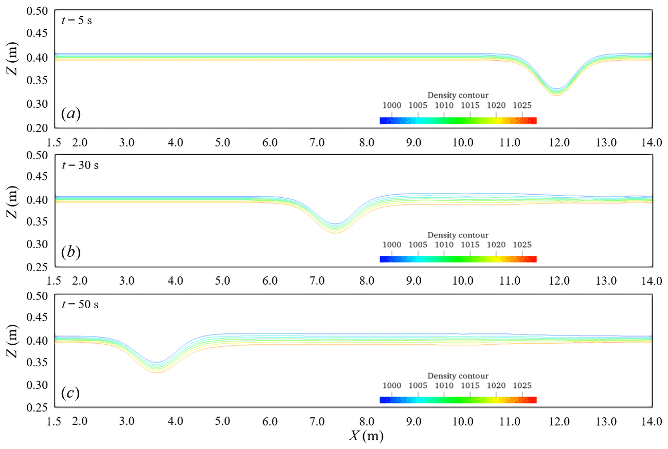
Figure 7 shows the density contours at three different times from Case Flat_4 in the laboratory experiment of Hsieh and coworkers, showing the stable evolution of an ISW. The results also show the realistic evolution of the thickening of the pycnocline after ISW propagation because of convection and diffusion. At the same time, the propagation of the ISW is stable and unbroken.
To further verify the model, the waveform is compared between the numerical simulations and the experimental measurements, and the measurement point selection is the same as the experimental setting, as shown in Fig. 6. Figure 8 shows the comparison results between the waveform simulated by ISWFoam and the experimental results at probes P1–P5. Figure 8 shows that the results of the numerical simulations agree with the experimental results (red circle). Notably, the laboratory wave height at the probe P1 measurement point is greater than the numerical simulation results, and the wave surface of the laboratory wave is not smooth, which is caused by the wave generation method using the gravity collapse mechanism in the laboratory. In general, the model developed in this paper can simulate the generation and evolution of ISWs in continuously stratified fluids.

Figure 8Comparison of the waveform between the experimental results and numerical simulation results at probes P1–P5.
4.2 ISW propagating over a submerged triangular ridge
4.2.1 Experimental data used
In this section, the validation of the numerical model is conducted through an ISW propagating over a submerged triangular ridge with the continuously stratified experiments described in Hsieh et al. (2015). The laboratory tank is 12 m long and has a stable water depth of 0.5 m, with which the fluid system has a finite thickness of the pycnocline. The specific experimental parameters used for validation of ISWFoam include the various depths of the upper (h1) and lower (h2) layers; the fluid density of the upper (ρ1) and lower (ρ2) layers of 996 kg m−3 and 1030 kg m−3, respectively; the ISW amplitude (α=0.056 m); the location of the centre of the pycnocline (zpyc=0.4 m); the thickness of the pycnocline (dpyc=0.04 m vertically); the height of the isosceles triangular ridge (hs=0.30 m vertically); and the slope angle of the ridge for α=45∘. The physical dimensions, and ultrasonic probe locations in the experiments of Hsieh et al. (2015), as shown in Fig. 9, are adopted to establish the numerical computation domain.
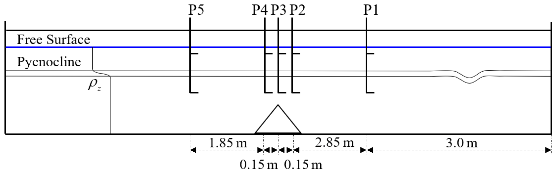
Figure 9Schematic illustration of the laboratory set-up and the locations of the probes (Hsieh et al., 2015).
4.2.2 Numerical implementation
The numerical tank is designed to reproduce the experiment described in Fig. 9. The unstructured grid and local mesh refinement based on the finite-volume method are used to construct the computational domain and discretise the governing equations. The grid is uniform in the x direction, y direction and z direction, and the sizes are m, m and m, respectively. The precise grid described triangular ridge section is m, m and m at the slope, as shown in Fig. 10. The sponge layer on both sides, whose length is double the wave characteristic length defined through integration of the wave profile in Sect. 3 for this case, has been checked to absorb the reflected wave well. Rigid wall conditions are applied to both sides, while the slip and slip conditions are assigned to the bottom and the surface of the submerged ridge boundaries, respectively. The top boundary is a rigid lid. The inlet and outlet boundaries adopt cyclic boundary conditions. The boundary conditions related to the density field are no-flux boundary conditions.
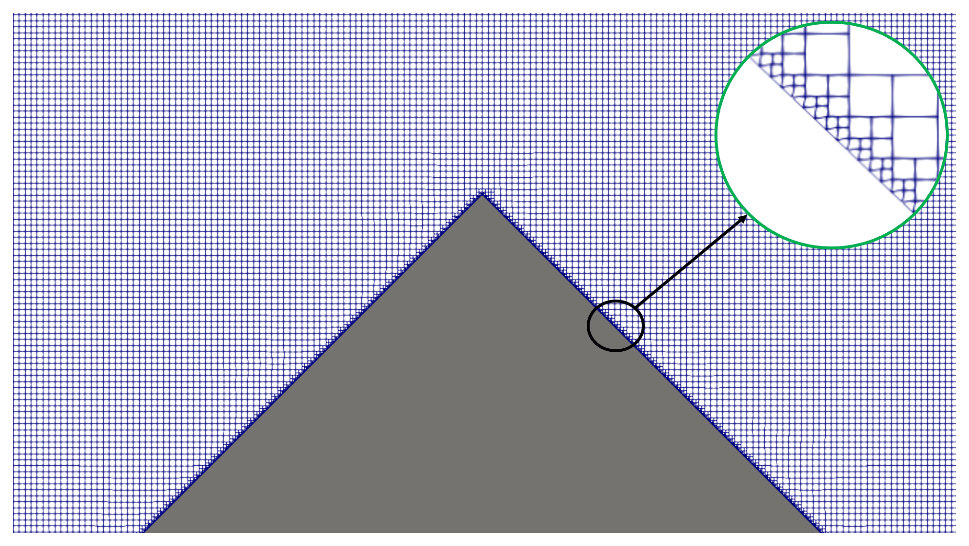
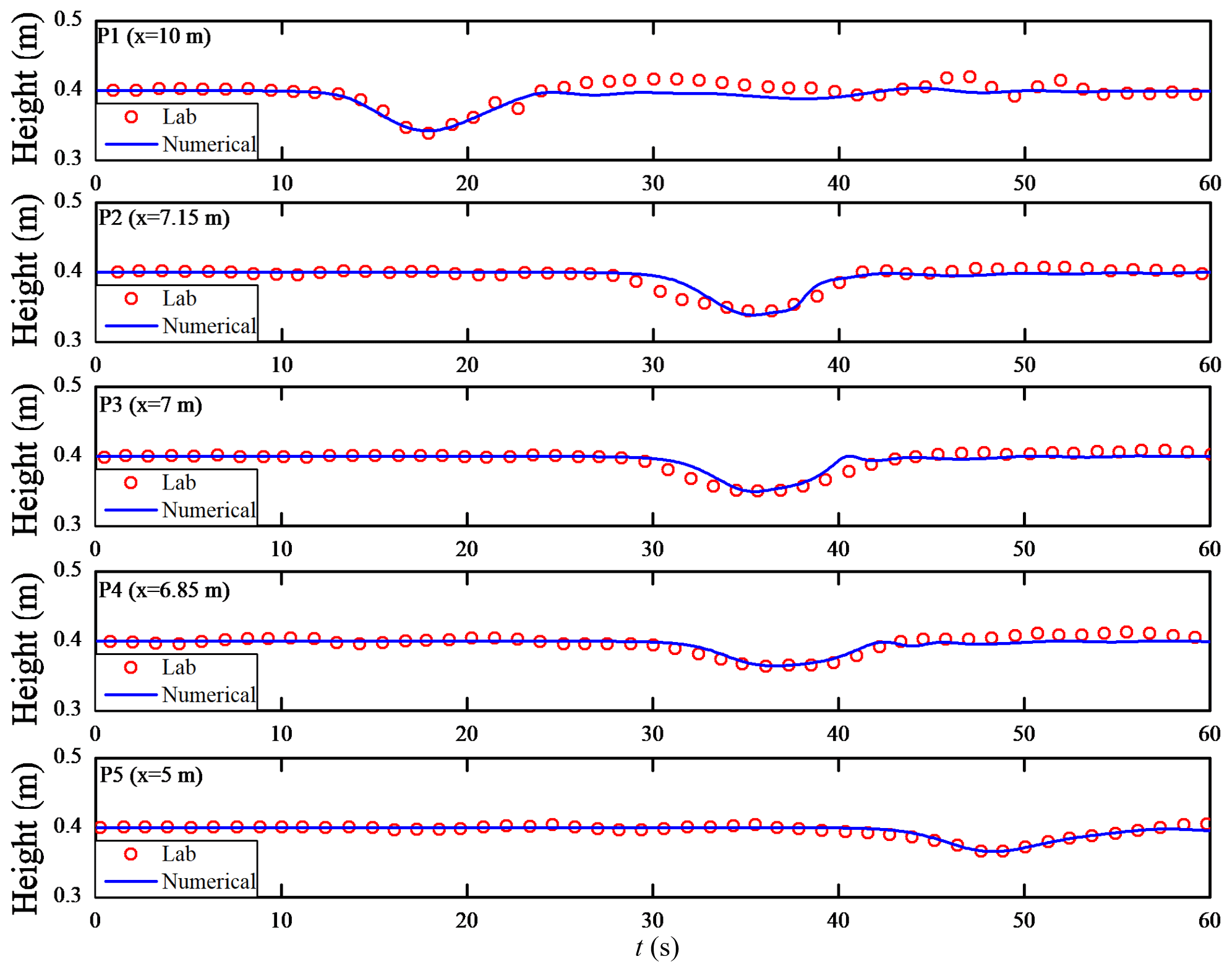
Figure 11Comparison of the waveform between the experimental results in Hsieh et al. (2015) and numerical simulation results at probes P1–P5.
4.2.3 Comparisons between the numerical and experimental results
Figure 11 shows the comparison results between the waveform calculated by ISWFoam and the experimental results at probes P1–P5. In each subplot, the results of the numerical simulations (blue line) are found to be in good agreement with the experimental results (red circle). From Fig. 11a, the numerical simulation result of the probe P1 measurement after 20 s is different from the experimental results, which is caused by the different ISW generation methods. For the experimental results, the first large leading ISW is formed via the gravity collapse mechanism, which is trailed by a train of small-amplitude mode-one waves that is generated due to shear instabilities. However, the initialisation method used to generate an initial ISW for the numerical simulation in this paper is more stable than the gravity collapse mechanism, so the rear part of the ISW is relatively flat compared to the experimental results for probe P1. In Fig. 11, the waveform of the ISW gradually evolves towards a flat waveform due to the interaction between the ISW and the ridge. In general, the model developed in this paper can simulate the interaction between ISWs and structures.
4.3 ISW propagating on a slope
To verify the ability and accuracy of simulating the ISW breaking of the numerical model, two continuously stratified laboratory experiments (12 and 15) of Michallet and Ivey (1999) are chosen for the simulation in this section. The experimental set-up is represented schematically in Fig. 12. We set up a numerical tank of the experiment of Michallet and Ivey (1999), which includes a tank that is L=4.2 m long, 0.25 m wide and has a water depth of 0.15 m. The layer thickness ratio varies from 0.60 to 0.91. A linear slope s=0.214 starts at 0.7 m from the right end of the tank for experiments 12 and 15. The grid is uniform in the x direction, y direction and z direction, and the sizes are m, m and m, respectively. The precise grid describing the slope section is m and m at the slope.
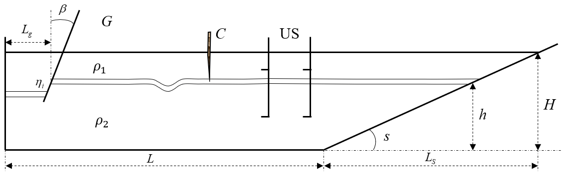
Figure 12Schematic diagram of the laboratory set-up.“C” and “US” represent the experimental devices at the probes.
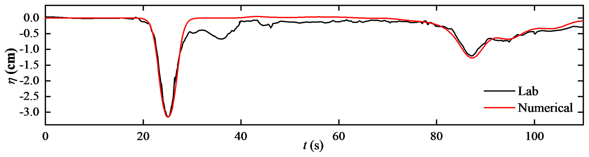
Figure 13Time series of the interface displacement. The probe was 99.8 cm away from the start of the slope.
The sponge layer on the left side, whose length is double the wave characteristic length, is checked to properly dissipate the reflected wave. Slip boundary conditions are applied to the bottom and both sides, while slip boundary conditions are assigned to the top boundaries. The boundary conditions related to the density field are no-flux boundary conditions.
The vertical profile of the initial density is given by a hyperbolic tangent function profile
where z is the vertical position, kg m−3 is the base density field, Δρ is the change in the density, zpyc is the location of the centre of the pycnocline, and dpyc is the thickness of the pycnocline.
4.3.1 Case one and results
The first case of model verification is experiment 12 of Michallet and Ivey (1999) in this section. The layer thickness ratio is 0.84, and the density change (Δρ) value is 14 kg m−3. Figure 13 presents the time series for the interface displacement (ζ) for experiment 12 of Michallet and Ivey (1999). The results indicate reasonably good agreement between the time series of the simulated interface displacement and that of the laboratory results. The first trough centred around t=25 s represents the incident ISW propagating the probe 99.8 cm away from the start of the slope. The second trough centred at approximately t=87 s represents the reflected ISW at the generation side, which has a smaller amplitude and a longer wavelength than the incident ISW as the energy in the wave decreases. As shown in Fig. 13, the smooth waveform of the incident ISW of the numerical simulation indicates that the initialisation method of wave generation in this paper is more stable than the experiment.
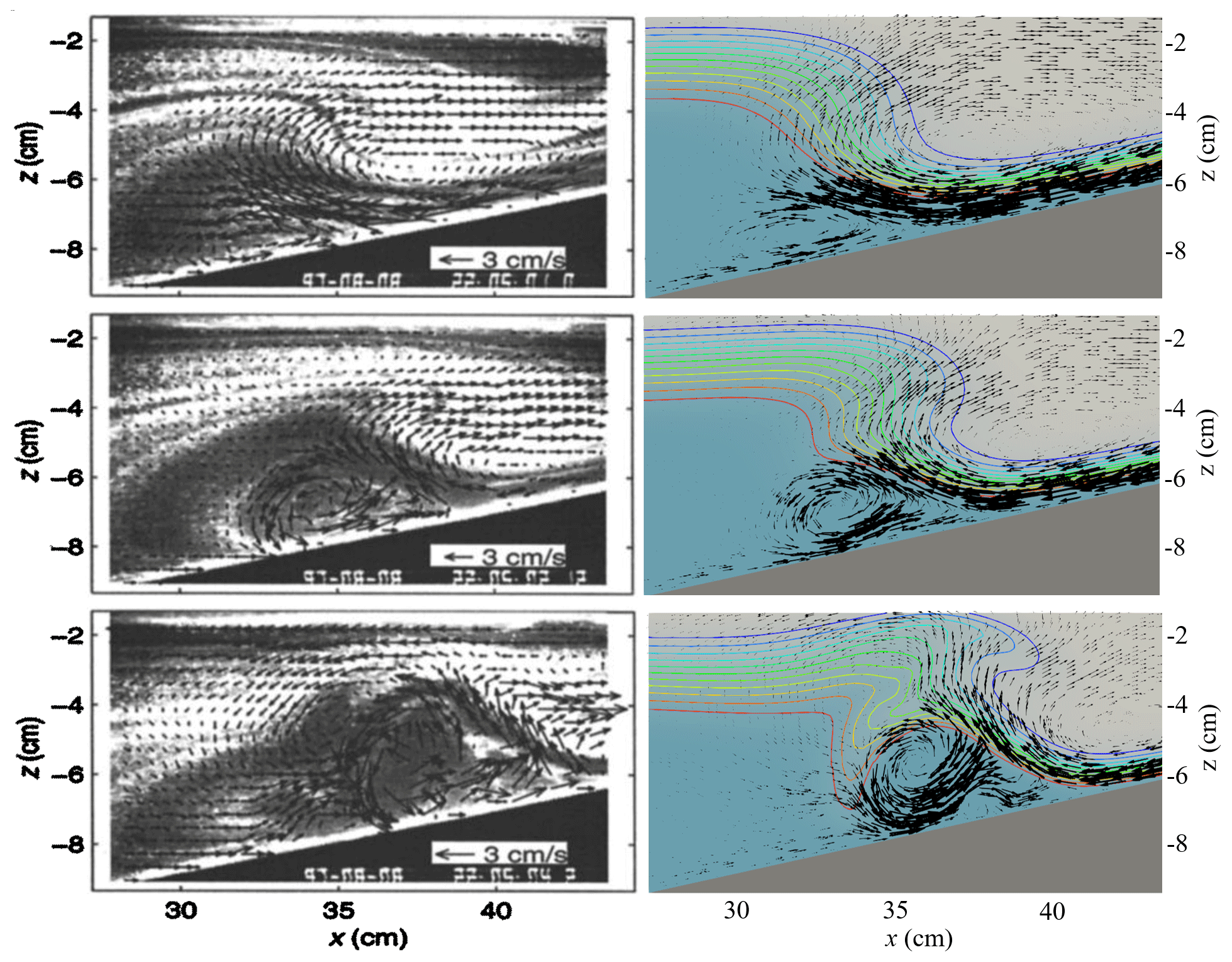
Figure 14Comparison of the velocity field between the experimental observation results in Michallet and Ivey (1999) (left) and numerical simulation results (right).
Figure 14 shows a comparison of ISWFoam results and the experimental observations of the velocity field associated with the ISW run-up process along the slope. The model effectively reproduces laboratory tests, such as the intensity and direction of the velocity field, the location of the vortices and the occurrence of boundary-layer separation beneath the ISW. Therefore, the model developed in this paper can reflect the ISW breaking phenomenon during the propagation of ISWs along the slope.
4.3.2 Case two and results
Another laboratory experiment that more clearly shows the ISW breaking phenomenon from Experiment 15 of Michallet and Ivey (1999) is used to verify the numerical model presented in this paper, and the corresponding numerical case is set corresponding to it. The layer thickness ratio is 0.77, and the density change (Δρ) value is 47 kg m−3. The wave amplitude and phase velocity at the slope calculated by ISWFoam are m and m s−1, which fit well with the experimental results of m and m s−1.
Figure 15 shows the results of the numerical simulations of the ISWs propagating along the slope and wave breaking using ISWFoam. As the ISW propagates to the slope, according to the conservation of mass, the upper fluid forward and the downward velocity of the lower fluid increasing along the slope results in the formation of a thin boundary layer, as shown in Fig. 15a, b and c. At the same time, the amplitude of the ISW increases, and the rear of the ISW gradually becomes very steep but does not overturn. With the development of the ISW, the rear waveform of the ISW cannot maintain its stability and overturns forward, resulting in wave breaking, as shown in Fig. 15d. After wave breaking occurs, the denser lower layer flow accelerates into the less dense upper layer flow, forming a mixture region, as shown in Fig. 15e. After the lower layer flow is drawn downward from beneath the ISW, a mixing region comprised of vortices is pushed upwards along the slope while the leading waveform is reflected, as shown in Fig. 15f, g and h. Figure 15i and j show the falling process of ISWs. From the perspective of the entire process of wave breaking, the steepening of the rear waveform in this case is the main reason for wave breaking.
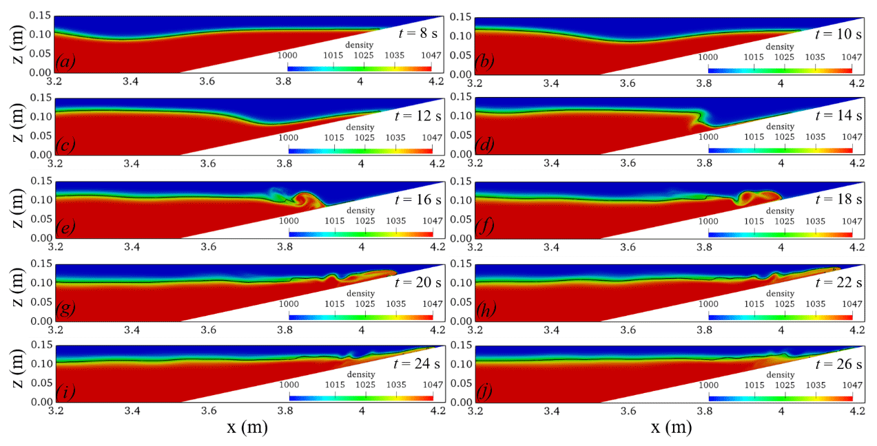
Figure 15Temporal and spatial variations in the ISWs breaking calculated using ISWFoam (the black line represents the waveform).
For comparison with the flow visualisation image of the experiment, a specified thickness of the pycnocline is presented, and the pycnocline ranges from 1003 to 1045 kg m−3 with dark colours as shown in Fig. 16.
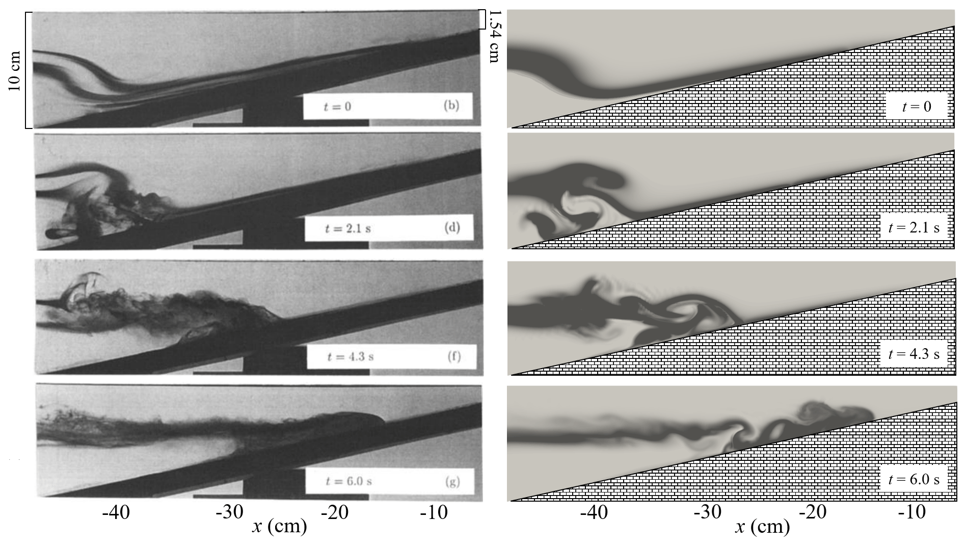
Figure 16Comparison of the density fields between the experimental observation results in Michallet and Ivey (1999) (left) and the numerical simulation results (right).
Figure 16 compares the ISWFoam results and the experimental results of Michallet and Ivey (1999) before, during and after ISW breaking. The results indicate that some main features of the laboratory tests are reasonably well reproduced by ISWFoam, such as the profile of ISW, the location of the wave breaking point, ISW arrival time, and spatial and temporal changes in the mixture region. Therefore, the model developed in this paper can accurately simulate the ISW breaking phenomenon during the propagation of ISWs along the slope.
The ISWFoam model developed in the present paper can be used as a tool to investigate the interaction between ISWs and complex structures and topography. In this section, two numerical examples are presented to show the capability of ISWFoam on field-scale simulation.
5.1 ISW propagating over a 3D Gaussian ridge
We designed a case of an ISW propagating over a 3D Gaussian ridge. The 3D Gaussian ridge is obtained by rotating a 2D Gaussian ridge:
where a is the ridge amplitude, and l is the standard deviation. With a=100 m and l=10, we can obtain a 2D Gaussian ridge with a height of 100 m and a bottom width of 40 m. Subsequently, the 3D Gaussian ridge can be obtained after a vertical rotation of 180∘.
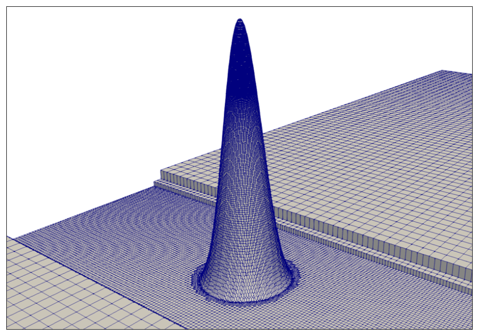
We set up a 3D numerical tank, which includes a tank that is 3 km long, 400 m wide (y direction from −200 to 200 m) and has a water depth of 120 m. The depths of the upper (h1) and lower (h2) layers are 20 and 100 m, respectively; the densities of the upper and lower layers are 1000 and 1030 kg m−3, respectively; the location of the centre of the pycnocline (zpyc) is 100 m; the pycnocline thickness (dpyc) is 1.5 m vertically; and the ISW amplitude a is 20 m. The Gaussian ridge is located at 800 m horizontally. The grid is gradually changed from Δx=20 m to Δx=2.5 m in the x direction, the grids in the y direction are uniform with a constant cell width of Δy=2.5 m, and the grids in the z direction are non-uniform, with a minimum cell height of Δz=1 m near the interface of the ISW. The precise grid described the 3D Gaussian ridge section as m, m and m, as shown in Fig. 17. The sponge layer on both sides, whose length is the double wave characteristic length, has been checked to properly dissipate the reflected wave. Slip boundary conditions are applied to the bottom and both sides, while cyclic boundary conditions are assigned to the inlet and outlet boundaries. The top boundary is a rigid lid. The boundary conditions related to the density field are no-flux boundary conditions.
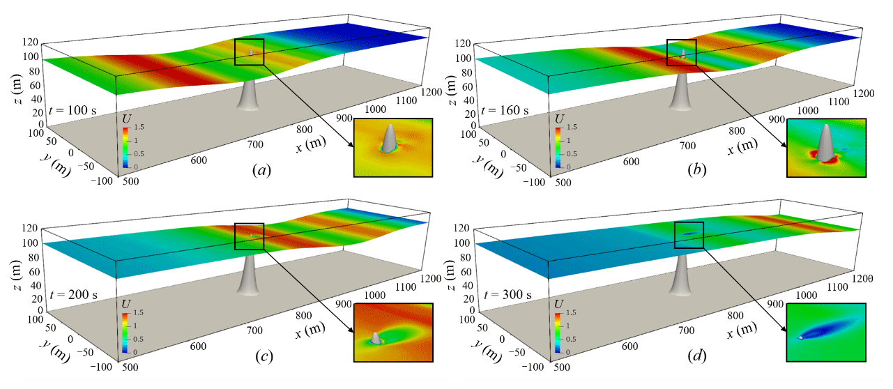
Figure 18 shows the temporal and spatial variations in the ISWs propagating over a 3D Gaussian ridge. The ISW reaches the Gaussian ridge, causing the wave surface in front of the ridge to decrease, and the wave surface behind the ridge to climb up the ridge, as shown in Fig. 18a. Due to being obstructed by the Gaussian ridge, flow around a ridge and wave surface uplift are generated on both sides of the Gaussian ridge (perpendicular to the direction of wave propagation), as shown in Fig. 18b. As the ISW propagated over the Gaussian ridge, the wave surface climbed along the ridge, and at the same time, low velocity was generated behind the ridge, as shown in Fig. 18c. Since the top of the ridge is in the pycnocline, there will be a low-velocity area behind the ridge for a period of time after the ISW passes, as shown in Fig. 18d. In general, the ISWFoam model with unstructured grids and local mesh refinement can simulate the interaction between ISWs and complex structures and topography at the field scale.
5.2 ISW propagating over a hyperbolic tangent terrain
The propagation of ISWs to the shore is bound to be affected by the continental shelf, and shallow water evolution phenomena such as nonlinear evolution, breaking phenomena and waveform inversion occur on the undulating continental shelf. For simplicity, this section simplifies the continental shelf into a hyperbolic tangent terrain, and the terrain profile formula is as follows (Lamb, 2002):
where aT is the ridge amplitude, which is 60 m; l is the width of the continental shelf change area, which is 200 m; and x and z are the horizontal and vertical coordinate positions, respectively.
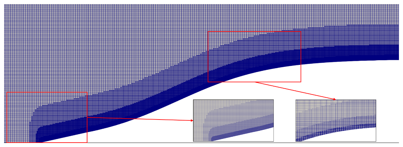
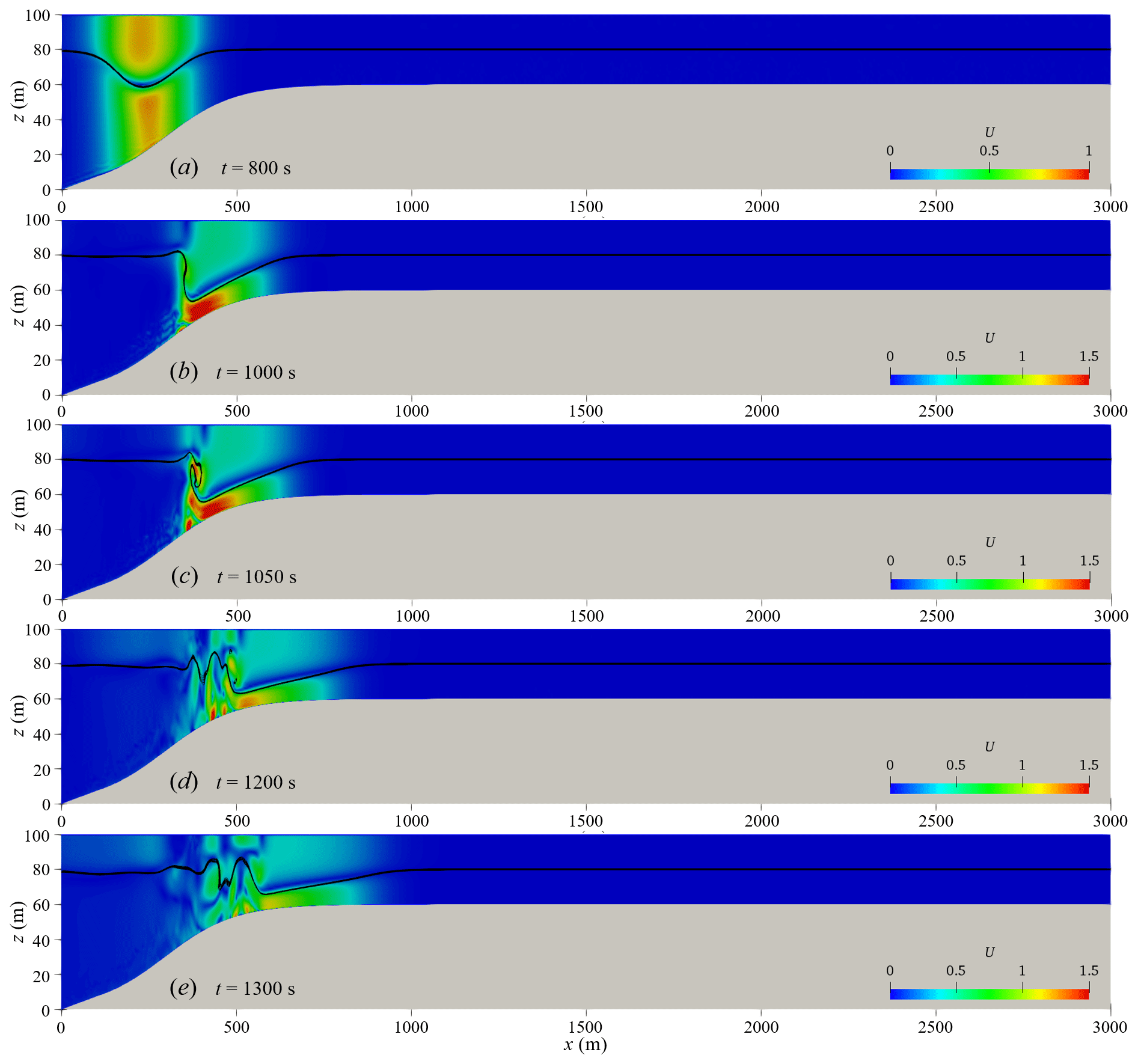
Figure 20Velocity field diagram of ISW propagation (the black solid line is the iso-density contours, t=800 to 1300 s).
We set up a 3D numerical tank, which includes a tank that is 7.5 km long, 200 m wide (y direction from −100 to 100 m) and has a water depth of 100 m (z direction from 0 to 100 m). The depths of the upper (h1) and lower (h2) layers are 20 and 80 m in the deep water, respectively, and the depths of the upper (h1) and lower (h2) layers are both 20 m in the shallow water. The densities of the upper and lower layers are 1000 and 1012 kg m−3, respectively; the pycnocline thickness (dpyc) is 2 m; the location of the pycnocline (zpyc) centre is at 80 m; and the ISW amplitude a is 20 m. The starting point of the hyperbolic tangent terrain is located at 0 m horizontally, and the top of the terrain is 40 m underwater. Therefore, ISWs will gradually propagate from a deep water area with a water depth of 100 m to a shallow water area with a water depth of 40 m. The horizontal grid is gradually changed from 40 m at the inlet to 4 m in the study area, and then from the study area to 60 m at the outlet, the grid is uniform in the y direction and z direction, which are 4 and 1 m. The hyperbolic tangent terrain is characterised by 4-level local mesh refinement, and the minimum grid size is 5 cm, as shown in Fig. 19. The sponge layer on both sides, whose length is double the characteristic wave length, has been checked to properly dissipate the reflected wave. Cyclic boundary conditions are assigned to the inlet, outlet and both sides, while the slip and non-slip conditions are assigned to the bottom and the shelf topography. The top boundary is a rigid lid. The boundary conditions related to the density field are no-flux boundary conditions.
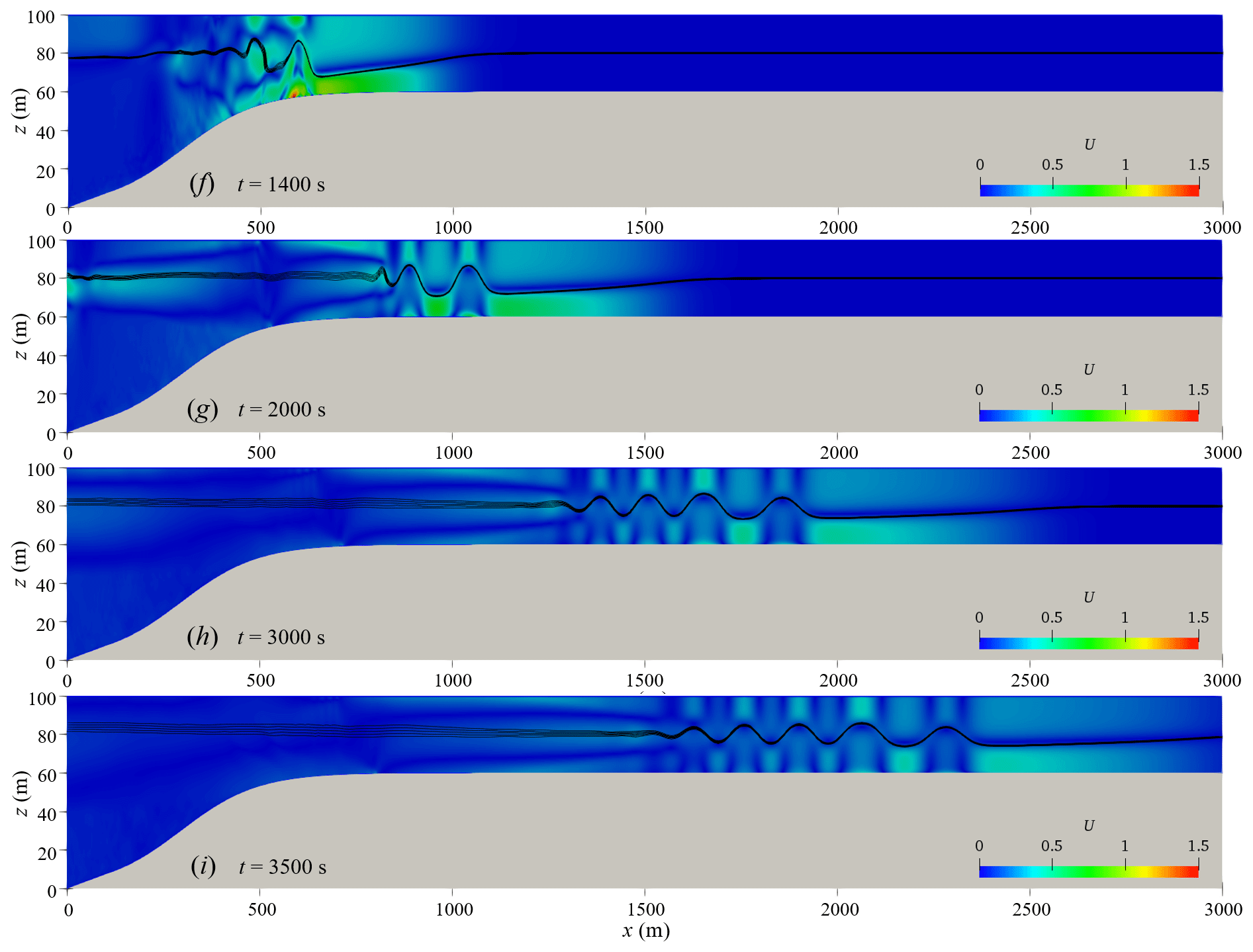
Figure 21Velocity field diagram of ISW propagation (the black solid line is the iso-density contours, t=1400 to 3500 s).
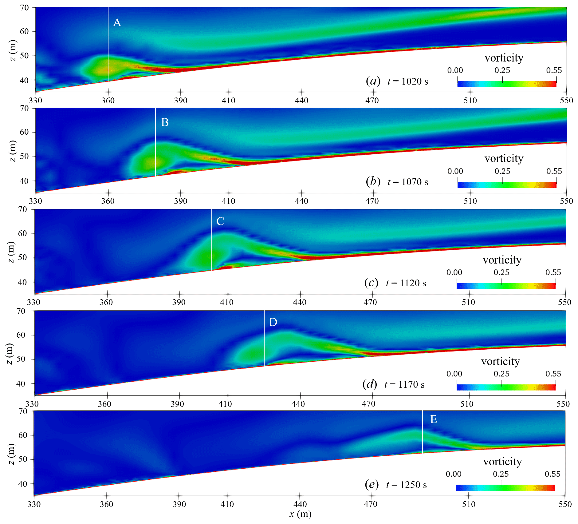
Figure 20 shows the waveform and velocity field when the ISW passes through the hyperbolic tangent terrain. From Fig. 20, it can be seen that the ISW breaks and has a significant waveform inversion when propagating from deep water of 100 m to shallow water of 40 m. As the ISWs propagate to the continental shelf, the water depth gradually becomes shallower, and the thickness of the lower fluid gradually decreases as shown in Fig. 20a. Due to the presence of the continental slope, the nonlinearity of the ISWs becomes stronger, and the trough velocity of the ISWs is significantly lower, which causes the waveform at the rear of the ISW to become steep, as shown in Fig. 20b. At the same time, the front waveform of the ISW gradually becomes flat and parallel to the shelf topography. As the waveform at the rear of the ISW becomes steeper and loses balance, the waveform at the rear of the ISW rolls forward, leading to the occurrence of ISW breaking phenomena, as shown in Fig. 20c. It is worth noting that the ISW breaking occurs at the rear of the ISW, while the front waveform does not break but transforms into another form of wave (referred to as the head wave) and continues to propagate steadily along the continental shelf. The breaking of ISWs causes severe disturbances in the water and excites a series of secondary waves at the tail of the head wave, represented by elevation ISWs (as shown in Fig. 20d, e), and then elevation ISWs propagate forward steadily in shallow water (as shown in Fig. 21g, h, i). The shelf slope of the case in this section is the same as the shelf slope of s8_c1c case studied by Lamb and Xiao (2014), both of which are 0.1. The research results of Lamb and Xiao (2014) show that waveform inversion of a depression ISW will occur at this shelf slope, and a series of elevation ISWs will be generated and propagate stably in shallow water. The simulated results have good agreement with that of Lamb and Xiao (2014).

The vortex structure has an important influence on the material transport at the bottom of the shelf, so it is very necessary to study the vortex structure when the ISW breaks. Figure 22 show the vorticity field of the ISW at the breaking stage. With the occurrence of ISW breaking, a significant anticlockwise vortex structure is generated below the waveform at the rear of the ISW, as shown in Fig. 22a. With the propagation of the head wave, the vortex climbs along the shelf, the vortex continues to develop horizontally and vertically during the upward climb, and the vertical scale is about one-third of the local water depth (as shown in Fig. 22b, c). As the vortex structure continues to climb, the vorticity decays, and the vortex structure gradually disappears, as shown in Fig. 22d and e. Combined with the velocity field in Fig. 20, it can be seen that the vorticity before and after the ISW breaks is the largest, and the vortex structure is the most obvious. As the wave train of elevation ISWs propagates steadily, the vortex structure climbs up the shelf and gradually disappears.
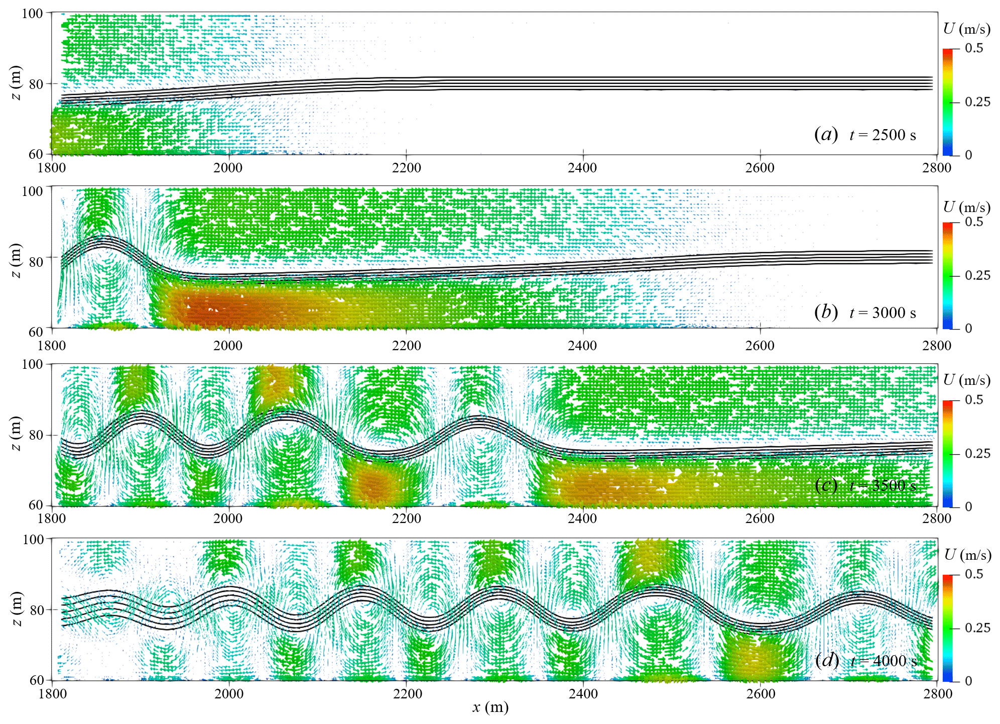
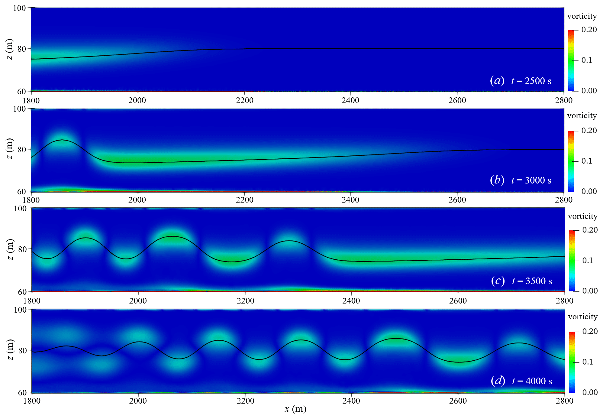
Figure 25Vorticity field of wave train in shallow water (the black solid line is the waveform).
In order to analyse the vortex of the three-dimensional structure, Fig. 23 show the vorticity field diagram on the transverse section, and the position of the transverse section corresponds to the marked section in Fig. 22. It can be seen from Fig. 23 that the vortex also evolves in the transverse section. Obviously, the bottom vortex structure generated by ISW breaking shows three-dimensional non-uniform features.
The velocity vector field of the head wave and the wave train of elevation ISWs in the shallow water area are shown in Fig. 24. The head wave generated by the breaking of the ISW loses the original wave shape of the ISW, the wave height becomes smaller, the wavelength becomes longer, and the velocity field is still in the form of upper layer forward and lower layer backward (as shown in Fig. 24a, b). In Fig. 24c and d, the velocity field and waveform of the entire wave train following the head wave are stable, the velocity field of each wave is backwards in the upper layer and forwards in the lower layer, and the wavelength gradually becomes longer as the wave train propagates. As the wave train propagates in shallow water, there is a large vorticity in the crest and trough areas of each wave, and it propagates forward steadily as the wave train propagates, as shown in Fig. 25. Generally, the waveform inversion and breaking phenomenon of ISWs is well indicated, and the propagation and evolution of the wave train generated by waveform inversion is also accurately described through ISWFoam simulation.
In this paper, a numerical model referred to as ISWFoam with a modified k–ω SST model, established by combining the density transport equation with a fully three-dimensional (3D) Navier–Stokes equation, is developed to simulate ISWs in continuously stratified, incompressible, viscous fluids based on the finite-volume method with unstructured grids and local mesh refinement of OpenFOAM. ISWFoam provides two initial wave generation methods to generate an ISW in continuously stratified fluids, including solving the weakly nonlinear models of the eKdV equation and the fully nonlinear models of the DJL equation. The verification process presents several applications, such as ISWs propagating on flat bottoms including laboratory scale and actual ocean scale, and ISWs over a submerged triangular ridge, a Gaussian ridge and slopes. The following conclusions were obtained as a result of this study.
ISWFoam using the finite-volume method with unstructured grids and local mesh refinement can accurately simulate the generation and evolution of ISWs, the ISW breaking phenomenon, waveform inversion of ISWs and the interaction between ISWs and complex structures and topography. The method of initialising the ISW using weakly nonlinear eKdV equation models requires a period of movement before the jump of the velocity field develops into a field with continuous changes in velocity. The DJL equation wave generation method that considers the vertical velocity and the horizontal velocity along the vertical gradient is better than the eKdV equation wave generation method that only provides the horizontal average velocity. Using ISWFoam to simulate an ISW with infinite wave length, the metric for the appropriate mesh size is given as follows: the dimensions of the horizontal grid are 1150th of the characteristic length, while the vertical grid takes 125th of the ISW amplitude.
The ISWFoam code developed in this article can be downloaded for free from https://doi.org/10.5281/zenodo.5069480 (Mr-trekking, 2021).
All data can be accessed by contacting the corresponding author Qinghe Zhang (qhzhang@tju.edu.cn).
QZ and JL jointly developed this numerical method to calculate internal solitary waves in continuously stratified fluids. JL developed the code. TC performed the computations. QZ and JL jointly analysed the calculation results and wrote the paper together.
The contact author has declared that neither they nor their co-authors have any competing interests.
Publisher's note: Copernicus Publications remains neutral with regard to jurisdictional claims in published maps and institutional affiliations.
This research has been supported by The National Key Research and Development Program of China (grant no. 2021YFB2601100) and the National Natural Science Foundation of China (grant no. 51509183).
This paper was edited by James Kelly and reviewed by two anonymous referees.
Alford, M. H., Lien, R. C., Simmons, H., Klymak, J., Ramp, S., Yang, Y. J., Tang, D., and Chang, M. H.: Speed and evolution of nonlinear internal waves transiting the South China Sea, J. Phys. Oceanogr., 40, 1338–1355, https://doi.org/10.1175/2010JPO4388.1, 2010.
Alford, M. H., MacKinnon, J. A., Nash, J. D., Simmons, H., Pickering, A., Klymak, J. M., and Beitzel, T.: Energy flux and dissipation in Luzon Strait: Two tales of two ridges, J. Phys. Oceanogr., 41, 2211–2222, https://doi.org/10.1175/JPO-D-11-073.1, 2011.
Alford, M. H., Peacock, T., MacKinnon, J. A., Nash, J. D., Buijsman, M. C., Centurioni, L. R., and Fu, K. H.: The formation and fate of internal waves in the South China Sea, Nature, 521, 65–69, https://doi.org/10.1038/nature14399, 2015.
Aghsaee, P., Boegman, L., and Lamb, K. G.: Breaking of shoaling internal solitary waves, J. Fluid Mech., 659, 289, https://doi.org/10.1017/S002211201000248X, 2010.
Aghsaee, P., Boegman, L., Diamessis, P. J., and Lamb, K. G.: Boundary-layer-separation-driven vortex shedding beneath internal solitary waves of depression, J. Fluid Mech., 690, 321, https://doi.org/10.1017/jfm.2011.432, 2012.
Apel, J., Ostrovsky, L., Stepanyants, Y., and Lynch, J. F.: Internal Solitons in the Ocean, Technical Report, Woods Hole Oceanographic Institution, https://doi.org/10.1575/1912/1070, 2006.
Bardina, J. E., Coakley, T. J., and Huang, P. G.: Turbulence Modeling Validation, Testing, and Development, NASA TM 110446, NASA Ames Research Center, Moffett Field, CA, USA, https://doi.org/10.2514/6.1997-2121, 1997.
Bell, J. B. and Marcus, D. L.: A second-order projection method for variable-density flows, J. Comput. Phys., 101, 334–348, https://doi.org/10.1016/0021-9991(92)90011-M, 1992.
Brown, D. J. and Christie, D. R.: Fully nonlinear solitary waves in continuously stratified incompressible Boussinesq fluids, Phys. Fluids, 10, 2569–2586, https://doi.org/10.1063/1.869771, 1998.
Boegman, L. and Stastna, M.: Sediment resuspension and transport by internal solitary waves, Annu. Rev. Fluid Mech., 51, 129–154, https://doi.org/10.1146/annurev-fluid-122316-045049, 2019.
Buijsman, M. C., McWilliams, J. C., and Jackson, C. R.: East-west asymmetry in nonlinear internal waves from Luzon Strait, J. Geophys. Res.-Oceans, 115, C10057, ,https://doi.org/10.1029/2009JC006004, 2010.
Cai, S., Xie, J., and He, J.: An overview of internal solitary waves in the South China Sea, Surv. Geophys., 33, 927–943, https://doi.org/10.1007/s10712-012-9176-0, 2012.
Cheng, M. H., Hwang, R. R., and Hsieh, C. M.: Numerical study on the transformation of an internal solitary wave propagating across a vertical cylinder, Appl. Ocean Res., 95, 102016, https://doi.org/10.1016/j.apor.2019.102016, 2020.
Choi, W. and Camassa, R.: Fully nonlinear internal waves in a two-fluid system, J. Fluid Mech., 396, 1–36, https://doi.org/10.1017/S0022112099005820, 1999.
Deshpande, S. S., Anumolu, L., and Trujillo, M. F.: Evaluating the performance of the two-phase flow solver interFoam, Computational Science & Discovery, 5, 014016, https://doi.org/10.1088/1749-4699/5/1/014016, 2012.
Diamessis, P. J., Domaradzki, J. A., and Hesthaven, J. S.: A spectral multidomain penalty method model for the simulation of high Reynolds number localized incompressible stratified turbulence, J. Comput. Phys., 202, 298–322, https://doi.org/10.1016/j.jcp.2004.07.007, 2005.
Ding, W., Ai, C., Jin, S., and Lin, J.: Numerical investigation of an internal solitary wave interaction with horizontal cylinders, Ocean Eng., 208, 107430, https://doi.org/10.1016/j.oceaneng.2020.107430, 2020.
Dunphy, M., Subich, C., and Stastna, M.: Spectral methods for internal waves: indistinguishable density profiles and double-humped solitary waves, Nonlin. Processes Geophys., 18, 351–358, https://doi.org/10.5194/npg-18-351-2011, 2011.
Farmer, D. M. and Smith, J. D.: Tidal interaction of stratified flow with a sill in Knight Inlet, Deep Sea Research Part A, Oceanographic Research Papers, 27, 239–254, https://doi.org/10.1016/0198-0149(80)90015-1, 1980.
Fringer, O. B., Gerritsen, M., and Street, R. L.: An unstructured-grid, finite-volume, nonhydrostatic, parallel coastal ocean simulator, Ocean Model., 14, 139–173, https://doi.org/10.1016/j.ocemod.2006.03.006, 2006.
Fu, D. M., You, Y. X., and Li, W.: Numerical simulation of internal solitary waves with a submerged body in a two-layer fluid, Ocean Engineering (Haiyang Gongcheng), 37, 38–44, 2009.
Gao, X. Y., You, Y. X., Wang, X., and Li, W.: Numerical simulation for the internal solitary wave based on MCC theory, Ocean Eng. (Haiyang Gongcheng), 30, 29–36, 2012.
Grimshaw, R., Pelinovsky, E., Talipova, T., and Kurkina, O.: Internal solitary waves: propagation, deformation and disintegration, Nonlin. Processes Geophys., 17, 633–649, https://doi.org/10.5194/npg-17-633-2010, 2010.
Guo, C. and Chen, X.: A review of internal solitary wave dynamics in the northern South China Sea, Prog. Oceanogr., 121, 7–23, https://doi.org/10.1016/j.pocean.2013.04.002, 2014.
Hallberg, R. and Rhines, P.: Buoyancy-driven circulation in an ocean basin with isopycnals intersecting the sloping boundary, J. Phys. Oceanogr., 26, 913–940, https://doi.org/10.1175/1520-0485(1996)026<0913:BDCIAO>2.0.CO;2, 1996.
Hallberg, R.: Stable split time stepping schemes for large-scale ocean modeling, J. Comput. Phys., 135, 54–65, https://doi.org/10.1006/jcph.1997.5734, 1997.
Helfrich, K. R. and Melville, W. K.: Long nonlinear internal waves, Annu. Rev. Fluid Mech., 38, 395–425, https://doi.org/10.1146/annurev.fluid.38.050304.092129, 2006.
Hsieh, C. M., Hwang, R. R., Hsu, J. R. C., and Cheng, M. H.: Flow evolution of an internal solitary wave generated by gravity collapse, Appl. Ocean Res., 48, 277–291, https://doi.org/10.1016/j.apor.2014.10.001, 2014.
Hsieh, C. M., Hwang, R. R., Hsu, J. R. C., and Cheng, M. H.: Numerical modeling of flow evolution for an internal solitary wave propagating over a submerged ridge, Wave Motion, 55, 48–72, https://doi.org/10.1016/j.wavemoti.2014.12.008, 2015.
Huthnance, J. M.: Waves and currents near the continental shelf edge, Prog. Oceanogr., 10, 193–226, https://doi.org/10.1016/0079-6611(81)90004-5, 1981.
Issa, R. I.: Solution of the implicitly discretised fluid flow equations by operator-splitting, J. Comput. Phys., 62, 40–65, https://doi.org/10.1016/0021-9991(86)90099-9, 1986.
Jasak, H.: Error Analysis and Estimation for the Finite Volume Method with Applications to Fluid Flows, PhD thesis, Imperial College London, 1996.
Ko, D. S., Martin, P. J., Rowley, C. D., and Preller, R. H.: A real-time coastal ocean prediction experiment for MREA04, J. Marine Syst., 69, 17–28, https://doi.org/10.1016/j.jmarsys.2007.02.022, 2008.
Lamb, K. G.: Numerical experiments of internal wave generation by strong tidal flow across a finite amplitude bank edge, J. Geophys. Res.-Oceans, 99, 843–864, https://doi.org/10.1029/93JC02514, 1994.
Lamb, K. G. and Yan, L.: The evolution of internal wave undular bores: comparisons of a fully nonlinear numerical model with weakly nonlinear theory, J. Phys. Oceanogr., 26, 2712–2734, https://doi.org/10.1175/1520-0485(1996)026<2712:TEOIWU>2.0.CO;2, 1996.
Lamb, K. G.: A numerical investigation of solitary internal waves with trapped cores formed via shoaling, J. Fluid Mech., 451, 109–144, doi.org/10.1017/S002211200100636X, 2002.
Lamb, K. G. and Nguyen, V. T.: Calculating energy flux in internal solitary waves with an application to reflectance, J. Phys. Oceanogr., 39, 559–580, https://doi.org/10.1175/2008JPO3882.1, 2009.
Lamb, K. G.: Energy and pseudoenergy flux in the internal wave field generated by tidal flow over topography, Cont. Shelf Res., 27, 1208–1232, https://doi.org/10.1016/j.csr.2007.01.020, 2007.
Lamb, K. G. and Xiao, W.: Internal solitary waves shoaling onto a shelf: Comparisons of weakly-nonlinear and fully nonlinear models for hyperbolic-tangent stratifications, Ocean Model., 78, 17–34, https://doi.org/10.1016/j.ocemod.2014.02.005, 2014.
Li, J. Y., Zhang, Q. H., and Chen, T. Q.: Numerical Simulation of Internal Solitary Wave in Continuously Stratified Fluid, Journal of Tianjin University (Sci. Tech.), 54, 161–170, 2021.
Li, Q. and Farmer, D. M.: The generation and evolution of nonlinear internal waves in the deep basin of the South China Sea, J. Phys. Oceanogr., 41, 1345–1363, https://doi.org/10.1175/2011JPO4587.1, 2011.
Li, Z., You, Y. U., Zhe, S., Zang, J. M., Li, Z. H., and Yu, Z. B.: CFD Simulation of Internal Solitary Wave Using the Volume-of-fluid Method within OpenFOAM, DEStech Transactions on Computer Science and Engineering, https://doi.org/10.12783/dtcse/mmsta2017/19617, 2017.
Long, R. R.: Some aspects of the flow of stratified fluids: I. A theoretical investigation, Tellus, 5, 42–58, https://doi.org/10.1111/j.2153-3490.1953.tb01035.x, 1953.
Meng, Q. and Zhang, C.: A third-order KdV solution for internal solitary waves and its application in the numerical wave tank, Journal of Ocean Engineering and Science, 1, 93–108, https://doi.org/10.1016/j.joes.2016.03.002, 2016.
Menter, F. R., Kuntz, M., and Langtry, R.: Ten years of industrial experience with the SST turbulence model, Turbulence, Heat. Mass Transfer, 4, 625–632, 2003.
Michallet, H. and Ivey, G. N.: Experiments on mixing due to internal solitary waves breaking on uniform slopes, J. Geophys. Res.-Oceans, 104, 13467–13477, https://doi.org/10.1029/1999JC900037, 1999.
Miyata, M.: An internal solitary wave of large amplitude, La Mer, 23, 43–48, 1985.
Miyata, M.: Long Internal Waves of Large Amplitude, Springer, Berlin, 399–406, https://doi.org/10.1007/978-3-642-83331-1_44, 1988.
Mr-trekking: Mr-trekking/ISW: ISWFOAM v1.1.1, Zenodo [code], https://doi.org/10.5281/zenodo.5069480, 2021.
OpenFOAM: User Guide, http://www.openfoam.com/documentation/user-guide (last access: 12 December 2021), 2019.
Osborne, A. R. and Burch, T. L.: Internal solitons in the Andaman Sea, Science, 208, 451–460, https://doi.org/10.1126/science.208.4443.451, 1980.
Rayson, M. D., Ivey, G. N., Jones, N. L., and Fringer, O. B.: Resolving high-frequency internal waves generated at an isolated coral atoll using an unstructured grid ocean model, Ocean Model., 122, 67–84, https://doi.org/10.1016/j.ocemod.2017.12.007, 2018.
Sandstrom, H. and Elliott, J. A.: Internal tide and solitons on the Scotian Shelf: A nutrient pump at work, J. Geophys. Res.-Oceans, 89, 6415–6426, https://doi.org/10.1029/JC089iC04p06415, 1984.
Shaw, P. T., Ko, D. S., and Chao, S. Y.: Internal solitary waves induced by flow over a ridge: With applications to the northern South China Sea, J. Geophys. Res.-Oceans, 114, C02019, https://doi.org/10.1029/2008JC005007, 2009.
Simmons, H. L., Hallberg, R. W., and Arbic, B. K.: Internal wave generation in a global baroclinic tide model, Deep Sea Research Part II: Topical Studies in Oceanography, 51, 3043–3068, https://doi.org/10.1016/j.dsr2.2004.09.015, 2004.
Smedstad, O. M., Hurlburt, H. E., Metzger, E. J., Rhodes, R. C., Shriver, J. F., Wallcraft, A. J., and Kara, A. B.: An operational eddy resolving 1/16 global ocean nowcast/forecast system, J. Marine Syst., 40, 341–361, https://doi.org/10.1016/S0924-7963(03)00024-1, 2003.
Subich, C. J., Lamb, K. G., and Stastna, M.: Simulation of the Navier–Stokes equations in three dimensions with a spectral collocation method, Int. J. Numer. Meth. Fl., 73, 103–129, https://doi.org/10.1002/fld.3788, 2013.
Thiem, Ø., Carr, M., Berntsen, J., and Davies, P. A.: Numerical simulation of internal solitary wave-induced reverse flow and associated vortices in a shallow, two-layer fluid benthic boundary layer, Ocean Dynam., 61, 857, https://doi.org/10.1007/s10236-011-0396-5, 2011.
Turkington, B., Eydeland, A., and Wang, S.: A computational method for solitary internal waves in a continuously stratified fluid, Studies in Applied Mathematics, 85, 93–127, https://doi.org/10.1002/sapm199185293, 1991.
Vlasenko, V., Stashchuk, N., and Hutter, K.: Baroclinic Tides: Theoretical Modeling and Observational Evidence, Cambridge University Press, United Kingdom, https://doi.org/10.5670/oceanog.2006.107, 2005.
Vlasenko, V., Stashchuk, N., Guo, C., and Chen, X.: Multimodal structure of baroclinic tides in the South China Sea, Nonlinear Processes in Geophysics, 17, 529–543, https://doi.org/10.5194/npg-17-529-2010, 2010.
Wang, X., Zhou, J. F., Wang, Z., and You, Y. X.: A numerical and experimental study of internal solitary wave loads on semi-submersible platforms, Ocean Eng., 150, 298–308, https://doi.org/10.1016/j.oceaneng.2017.12.042, 2018.
Wilcox, D. C.: Comparison of two-equation turbulence models for boundary layers with pressure gradient, AIAA J., 31, 1414–1421, https://doi.org/10.2514/3.11790, 1993.
Xu, C. and Stastna, M.: Instability and cross-boundary-layer transport by shoaling internal waves over realistic slopes, J. Fluid Mech., 895, R6, https://doi.org/10.1017/jfm.2020.389, 2020.
Zhang, Z., Fringer, O. B., and Ramp, S. R.: Three-dimensional, nonhydrostatic numerical simulation of nonlinear internal wave generation and propagation in the South China Sea, J. Geophys. Res.-Oceans, 116, C05022, https://doi.org/10.1029/2010JC006424, 2011.
Zhang. H. G., Gu J. B., Jia, H. Q., and Gu, B.: A numerical model for internal wave propagation in continuously stratified ocean, Chinese Journal of Theoretical and Applied Mechanics, 44, 896–903, https://doi.org/10.6052/0459-1879-12-195, 2012.
- Abstract
- Introduction
- ISWFoam: A three-dimensional numerical solver for ISWs in a continuously stratified fluid
- Grid independence of the ISW simulation
- Model verification and results
- Simulation examples at the field scale
- Conclusions
- Code availability
- Data availability
- Author contributions
- Competing interests
- Disclaimer
- Financial support
- Review statement
- References