The Vertical City Weather Generator (VCWG v1.3.2)

The Vertical City Weather Generator (VCWG) is a computationally efficient urban microclimate model developed to predict temporal and vertical variation of potential temperature, wind speed, specific humidity, and turbulent kinetic energy. It is composed of various sub-models: a rural model, an urban vertical diffusion model, a radiation model, and a building energy model. Forced with weather data from a nearby rural site, the rural model is used to solve for the vertical profiles of potential temperature, specific humidity, and friction velocity at 10 m a.g.l. The rural model also calculates a horizontal pressure gradient. The rural model outputs are applied to a vertical diffusion urban microclimate model that solves vertical transport equations for potential temperature, momentum, specific humidity, and turbulent kinetic energy. The urban vertical diffusion model is also coupled to the radiation and building energy models using two-way interaction. The aerodynamic and thermal effects of urban elements, surface vegetation, and trees are considered. The predictions of the VCWG model are compared to observations of the Basel UrBan Boundary Layer Experiment (BUBBLE) microclimate field campaign for 8 months from December 2001 to July 2002. The model evaluation indicates that the VCWG predicts vertical profiles of meteorological variables in reasonable agreement with the field measurements. The average bias, root mean square error (RMSE), and R² for potential temperature are 0.25 K, 1.41 K, and 0.82, respectively. The average bias, RMSE, and R² for wind speed are 0.67 m s⁻¹, 1.06 m s⁻¹, and 0.41, respectively. The average bias, RMSE, and R² for specific humidity are 0.00057 kg kg⁻¹, 0.0010 kg kg⁻¹, and 0.85, respectively. In addition, the average bias, RMSE, and R² for the urban heat island (UHI) are 0.36 K, 1.2 K, and 0.35, respectively. Based on the evaluation, the model performance is comparable to the performance of similar models. The performance of the model is further explored to investigate the effects of urban configurations such as plan and frontal area densities, varying levels of vegetation, building energy configuration, radiation configuration, seasonal variations, and different climate zones on the model predictions. The results obtained from the explorations are reasonably consistent with previous studies in the literature, justifying the reliability and computational efficiency of VCWG for operational urban development projects.

1 Introduction

Urban areas interact with the atmosphere through various exchange processes of heat, momentum, and mass, which substantially impact human comfort, air quality, and energy consumption. Such complex interactions are observable from the urban canopy layer (UCL) to a few hundred meters within the atmospheric boundary layer (ABL; Britter and Hanna, 2003). Modeling enables a deeper understanding of interactions between urban areas and the atmosphere and can possibly offer solutions toward mitigating adverse effects of urban development on the climate. A brief review of modeling efforts is essential for more accurate model development toward an understanding of urban area–atmosphere interactions.

Mesoscale models incorporating the urban climate were initially aimed to resolve weather features with grid resolutions of at best a few hundred meters horizontally and a few meters vertically, without the functionality to resolve micro-scale three-dimensional flows or to account for atmospheric interactions with specific urban elements such as roads, roofs, and walls (Bornstein, 1975). These models usually consider the effect of built-up areas by introducing an urban aerodynamic roughness length (Grimmond and Oke, 1999) or adding source or sink terms in the momentum (e.g., drag term) and potential temperature (e.g., anthropogenic heat term) equations (Dupont et al., 2004). Therefore, if higher grid resolutions less than 10 m (horizontal and vertical) are desired (Moeng et al., 2007; Wang et al., 2009; Talbot et al., 2012), micro-scale climate models should be deployed. Recently, multi-scale climate models have coupled mesoscale and micro-scale models (Chen et al., 2011; Kochanski et al., 2015; Mauree et al., 2018). Numerous studies have used computational fluid dynamics (CFD) to investigate the urban microclimate while taking into account interactions between the atmosphere and urban elements with full three-dimensional flow analysis (Saneinejad et al., 2012; Blocken, 2015; Nazarian and Kleissl, 2016; Aliabadi et al., 2017; Nazarian et al., 2018). Despite accurate predictions, CFD models are not computationally efficient, particularly for weather forecasting at larger scales and for a long period of time, and they usually do not represent many processes in the real atmosphere such as clouds and precipitation. As an alternative, urban canopy models (UCMs) require understanding of the interactions between the atmosphere and urban elements to parameterize various exchange processes of radiation, momentum, heat, and moisture within and just above the canopy based on experimental data, physical processes from theoretical considerations, three-dimensional simulations, or simplified urban configurations (Masson, 2000; Kusaka et al., 2001; Martilli et al., 2002; Chin et al., 2005; Krayenhoff et al., 2014, 2015; Nazarian and Kleissl, 2016; Aliabadi et al., 2019). These urban canopy models are more computationally efficient than CFD models. They are designed to provide more details on heat storage and radiation exchange, while they employ less detailed flow calculations.

Urban microclimate models must account for a few unique features of the urban environment. Urban obstacles such as trees and buildings substantially contribute to changing flow and turbulence patterns in cities (Kastner-Klein et al., 2004). Difficulties arise when spatially inhomogeneous urban areas create highly three-dimensional wind patterns that result in the difficulty of parameterizations (Roth, 2000; Resler et al., 2017). For example, the surfaces of urban obstacles exert form and skin drag, consequently altering flow direction and producing eddies at different spatiotemporal scales. This can lead to the formation of shear layers at roof level with variable oscillation frequencies (Tseng et al., 2006; Masson et al., 2008; Zajic et al., 2011); all of such phenomena should be properly approximated in parameterizations.

Heat exchanges between indoor and outdoor environments significantly influence the urban microclimate. Various studies have attempted to parametrize heat sources and sinks caused by buildings such as heat fluxes due to infiltration, exfiltration, ventilation, walls, roofs, roads, windows, and building energy systems (e.g., condensers and exhaust stacks) (Kikegawa et al., 2003; Salamanca et al., 2010; Yaghoobian and Kleissl, 2012). Therefore, a building energy model (BEM) is required to be properly integrated into an urban microclimate model to take account of the impact of building energy performance on the urban microclimate (Bueno et al., 2011, 2012b; Gros et al., 2014). This two-way interaction between the urban microclimate and indoor environment can significantly affect the urban heat island (UHI) (K) and energy consumption of buildings (Salamanca et al., 2014).

Urban vegetation can substantially reduce the adverse effects of UHI (K), particularly during heat waves, resulting in improved thermal comfort (Grimmond et al., 1996; Akbari et al., 2001; Armson et al., 2012). Urban trees can potentially provide shade and shelter, therefore changing the energy balance of individual buildings in addition to the entire city (Akbari et al., 2001). A study of the local-scale surface energy balance revealed that the amount of energy dissipated due to the cooling effect of trees is not negligible and should be parameterized properly (Grimmond et al., 1996). In addition, the interaction between urban elements, most importantly trees and buildings, is evident in radiation trapping within the canyon and shading impact of trees (Krayenhoff et al., 2014; Redon et al., 2017; Broadbent et al., 2019). Buildings and trees obstruct the sky with implications for longwave and shortwave radiation fluxes both downward and upward that may create unpredictable diurnal and seasonal changes in UHI (K) (Kleerekoper et al., 2012; Yang and Li, 2015). Also, it has been shown that not only trees but also the fractional vegetation coverage on urban surfaces can alter urban temperatures with implications for UHI (K) (Armson et al., 2012). Trees, depending on their height and abundance relative to buildings, could also exert drag and alter flow patterns within the canopy; however, this effect is not as significant as the drag induced by buildings (Krayenhoff et al., 2015). Such complex interactions must be accounted for in successful urban microclimate models.

1.1 Research gaps

Numerous studies have focused on high-fidelity urban microclimate models with high spatiotemporal flow resolution, capturing important features of the urban microclimate with acceptable accuracy (Gowardhan et al., 2011; Soulhac et al., 2011; Blocken, 2015; Nazarian et al., 2018). Some example CFD models of this kind include Open-source Field Operation And Manipulation (OpenFOAM) (Aliabadi et al., 2017, 2018), the Parallelized Large-Eddy Simulation Model (PALM) (Maronga et al., 2015; Resler et al., 2017), and ENVI-met (Crank et al., 2018). Despite advances, however, high-fidelity models capable of resolving three-dimensional flows at micro-scale are not computationally efficient and are complex to implement for operational applications. As a remedy, lower-dimensional-flow urban microclimate models have been developed with many practical applications in city planning, architecture, and engineering consulting. For example, bulk flow (single-layer) models such as the Urban Weather Generator (UWG) calculate the flow dynamics in one point, usually the center of a hypothetical urban canyon, which is representative of all locations (Mills, 1997; Kusaka et al., 2001; Salamanca et al., 2010; Ryu et al., 2011; Bueno et al., 2012a, 2014). Another bulk flow (single-layer) model is the Canyon Air Temperature (CAT) model, which utilizes standard data from a meteorological station to estimate air temperature in a street canyon (Erell and Williamson, 2006). The Town Energy Balance (TEB) model calculates energy balances for urban surfaces and is forced by meteorological data and incoming solar radiation at the urban site on top of the modeling domain (Masson et al., 2002). The Temperatures of Urban Facets-3D (TUF-3D) model calculates urban surface temperatures with the main focus on three-dimensional radiation exchange, but it adopts bulk flow (single-layer) modeling, and it is forced by meteorological data on top of its domain (Krayenhoff and Voogt, 2007). More recently, TUF-3D was coupled to an Indoor–Outdoor Building Energy Simulator (TUF-3D-IOBES), but this model adopted a bulk flow (single-layer) parameterization (Yaghoobian and Kleissl, 2012). The multi-layer Building Effect Parametrization with Trees (BEP-Tree) model includes variable building heights, the vertical variation of climate variables, and the effects of trees, but it is not linked to a building energy model (Martilli et al., 2002; Krayenhoff, 2014; Krayenhoff et al., 2020). More recently, the BEP model has been coupled to a building energy model (BEP+BEM), but it is forced with meteorological variables from higher altitudes above a city using mesoscale models instead of near-surface meteorological variables measured outside the city (rural areas). An overview of the literature reveals an apparent paucity of independent urban microclimate models that account for spatiotemporal variations of meteorological parameters in the urban environment and consider the effects of trees, building energy, radiation, and the connection to the near-surface rural meteorological conditions measured outside a city, without the need for mesoscale modeling, that are computationally efficient and operationally simple for practical applications.

1.2 Objectives

In this study, we present a new urban microclimate model, called the Vertical City Weather Generator (VCWG), which attempts to overcome some of the limitations mentioned in the previous section. It resolves vertical profiles of climate variables, such as potential temperature, wind, specific humidity, and turbulent kinetic energy in relation to urban design parameters. VCWG also includes a building energy model. It allows parametric investigation of design options with urban climate control at multiple heights, particularly if multistory building design options are considered. This is a significant advantage over bulk flow (single-layer) models such as UWG, which only consider one point for flow dynamics inside a hypothetical canyon (Masson, 2000; Kusaka et al., 2001; Dupont et al., 2004; Krayenhoff and Voogt, 2007; Lee and Park, 2008; Bueno et al., 2012a, 2014). The advantages of VCWG are as follows. (1) It does not need to be coupled to a mesoscale weather model because it functions stand-alone as a microclimate model. (2) Unlike many UCMs that are forced with climate variables above the urban roughness sublayer (e.g., TUF-3D), VCWG is forced with rural climate variables measured at 2 m a.g.l. (temperature and humidity) and 10 m a.g.l. (wind) that are widely accessible and available around the world, making VCWG highly practical for urban design investigations in different climates. Further, unlike UWG, VCWG uses the Monin–Obukhov similarity theory in the rural area to consider effects of thermal stability and aerodynamic, temperature, and specific humidity roughness lengths to establish vertical profiles of potential temperature and specific humidity. (3) VCWG provides urban climate information in one dimension, i.e., resolved vertically, which is advantageous over bulk flow (single-layer) models. (4) VCWG is coupled with the building energy model using two-way interaction. (5) Unlike UWG, VCWG considers the effect of trees in the urban climate by modeling evapotranspiration (latent heat transfer), sensible heat transfer, radiation transfer, drag, and other processes due to trees.

The paper is structured as follows. Section 2 describes the methodology, outlining the components of the VCWG model and their connections: the forcing EnergyPlus^TM Weather (EPW) dataset, the rural model (RM), the one-dimensional vertical diffusion model, the building energy model, and the radiation model. This section also describes the location and details of the BUBBLE field campaign used for model evaluation. Section 3 provides the results and discussion. It starts with a detailed evaluation of VCWG by comparing simulation results with those of the BUBBLE field measurements. Then, results from other explorations, including effects of building dimensions, foliage density, building energy configuration, radiation configuration, seasonal variation, and different climate zones on the urban climate, are briefly presented with reference to the Supplement. Finally, Sect. 4 is devoted to conclusions and future work. Additional information about the sub-models and equations used is provided in Appendix A.

2 Methodology

2.1 Vertical City Weather Generator (VCWG)

Figure 1 shows the VCWG model schematic. VCWG consists of four integrated sub-models: (1) a rural model (RM) (Sect. 2.1.2) forces meteorological boundary conditions on VCWG based on Monin–Obukhov similarity theory (Paulson, 1970; Businger et al., 1971; Dyer, 1974) and a soil energy balance model (Bueno et al., 2012a, 2014); (2) an urban one-dimensional vertical diffusion model (Sect. 2.1.3) is used for calculation of the vertical profiles of urban microclimate variables including potential temperature, wind speed, specific humidity, and turbulent kinetic energy considering the effect of trees, buildings, and the building energy system (e.g., condensers and exhaust stacks). This model was initially developed by Santiago and Martilli (2010) and Simón-Moral et al. (2017), while it was later ingested into another model called the Building Effect Parametrization with Trees (BEP-Tree) model, considering the effects of trees (Krayenhoff, 2014; Krayenhoff et al., 2015, 2020). (3) A building energy model (BEM; Sect. 2.1.4) is used to determine the waste heat of buildings imposed on the urban environment. This model is a component of the Urban Weather Generator (UWG) model (Bueno et al., 2012a, 2014). (4) A radiation model with vegetation (Sect. 2.1.5) is used to compute the longwave and shortwave heat exchanges between the urban canyon, trees, and the atmosphere and sky. A summary of this model is provided by Meili et al. (2020) and the references within.

The sub-models are integrated to predict vertical variations of urban microclimate variables including potential temperature, wind speed, specific humidity, and turbulent kinetic energy as influenced by aerodynamic and thermal effects of urban elements including longwave and shortwave radiation exchanges, sensible heat fluxes released from urban elements, cooling effect of trees, and the induced drag by urban obstacles. The RM takes into account latitude, longitude, dry bulb temperature, relative humidity, dew point temperature and pressure at 2 m a.g.l., wind speed and direction at 10 m a.g.l., downwelling direct shortwave radiation, downwelling diffuse shortwave radiation, downwelling longwave radiation, and deep soil temperature from an EPW file. For every time step, and forced with the set of weather data, the RM then computes a potential temperature profile, a specific humidity profile, friction velocity, and a horizontal pressure gradient as a function of friction velocity, all of which are forced as boundary conditions to the one-dimensional vertical diffusion model in the urban area. The potential temperature and specific humidity are forced as fixed values on top of the domain for the urban vertical diffusion model in the temperature and specific humidity equations, respectively. The horizontal pressure gradient is forced as a source term for the urban vertical diffusion model in the momentum equation. It must be acknowledged that the model does not consider horizontal advection from the rural area. The model assumes that the rural site is upwind of the urban site and the top of the domain is above the urban boundary layer. While forced by the RM, the urban one-dimensional vertical diffusion model is also coupled with the building energy and radiation models. The three models have feedback interaction. The urban one-dimensional vertical diffusion model calculates the flow quantities at the center of control volumes, which are generated by splitting the urban computational domain into multiple layers within and above the urban canyon (see Fig. 2). The urban domain extends to 3 times the building height that conservatively falls closer to the top of the atmospheric roughness sublayer in the urban area (Santiago and Martilli, 2010; Aliabadi et al., 2017) but within the inertial layer in the rural area, where Monin–Obukhov similarity theory can be applied (Basu and Lacser, 2017). In VCWG, buildings with uniformly distributed height, equal width, and equal spacing from one another represent the urban area. The feedback interaction coupling scheme among the building energy model, radiation model, and the urban one-dimensional vertical diffusion model is designed to update the boundary conditions, surface temperatures, and the source and sink terms in the transport equations in successive time step iterations. More details about the sub-models are provided in the subsequent sections and Appendix A.

Figure 1 The schematic of the Vertical City Weather Generator (VCWG).

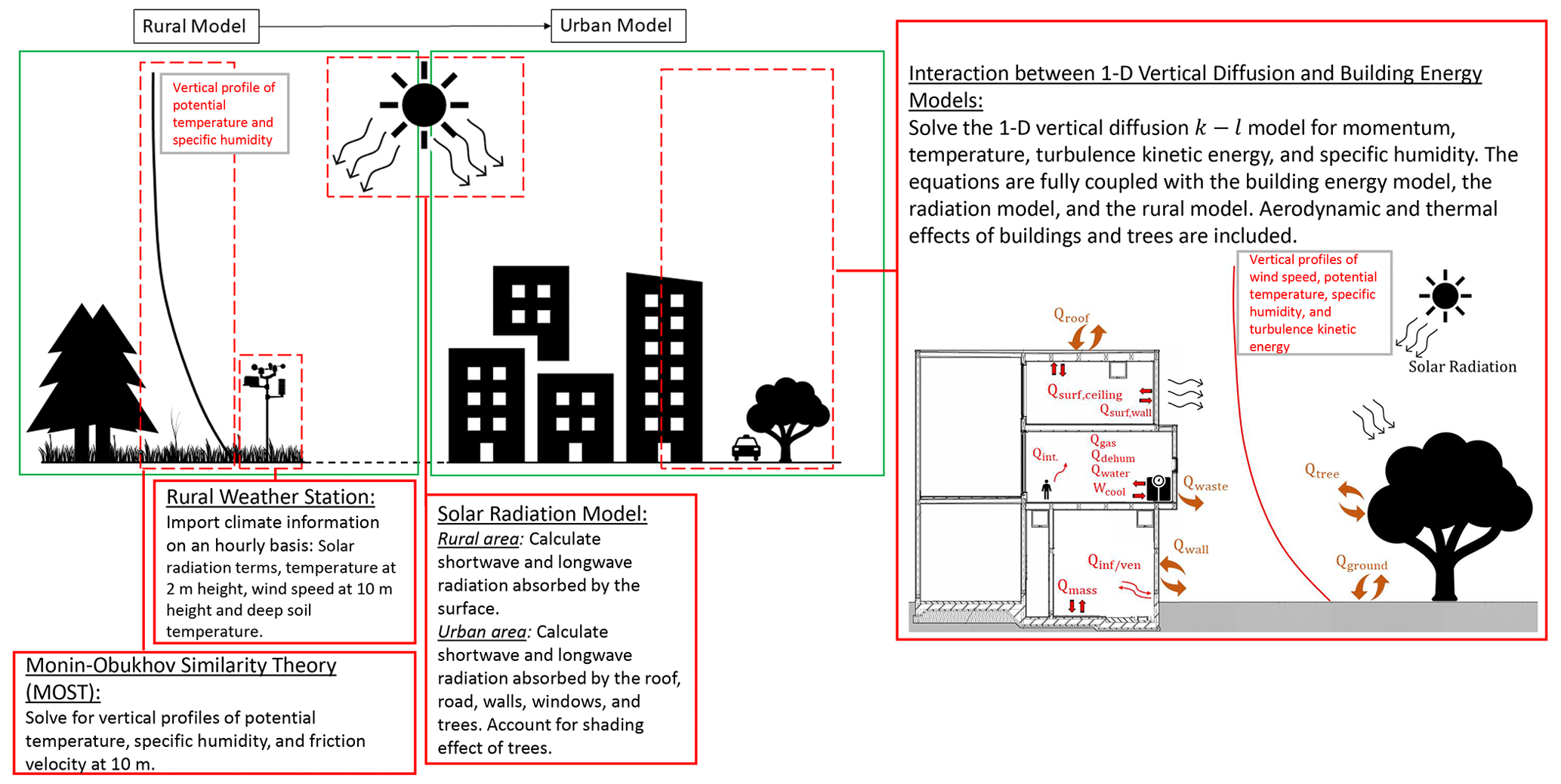
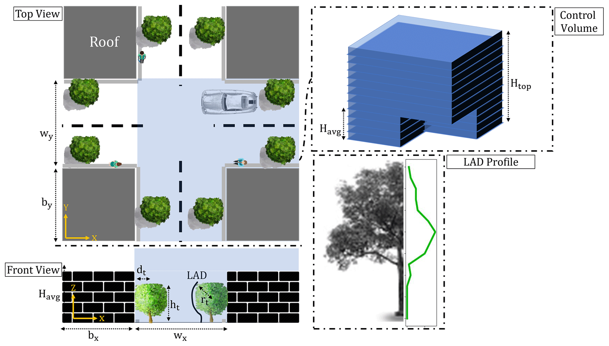
Figure 2 Simplified urban area used in VCWG and corresponding layers of control volumes within and above the canyon. The height of the domain is 3 times the average building height. A leaf area density (LAD) (m² m⁻³) profile is considered to represent trees.

2.1.1 EnergyPlus^TM weather data

Building energy and solar radiation simulations are typically carried out with standardized weather files. EPW files include recent weather data for 2100 locations and are saved in the standard EnergyPlus^TM format developed by the US Department of Energy (https://energyplus.net/weather, last access: 10 February 2021). The data are available for most North American cities, European cities, and other regions around the world. The weather data are arranged by the World Meteorological Organization (WMO) based on region and country. An EPW file contains typical hourly-based data for meteorological variables. The meteorological variables are dry bulb temperature, dew point temperature, relative humidity, incoming direct and diffusive shortwave radiation fluxes from the sun and sky, respectively, incoming longwave radiation flux, wind direction, wind speed, sky condition, precipitation (occasionally), deep soil temperature, and general information about field logistics and soil properties. Precipitation data are often missing in the EPW files.

2.1.2 Rural model

In the rural model, the Monin–Obukhov similarity theory (MOST) is used to solve for the vertical profiles of potential temperature, specific humidity, and friction velocity at 10 m a.g.l. using meteorological measurements near the surface. MOST is usually applied to the atmospheric surface layer over flat and homogeneous land to describe the vertical profiles of wind speed, potential temperature, and specific humidity as functions of momentum flux, sensible heat flux, and latent heat flux measured near the surface, respectively. Using MOST the gradient of potential temperature is given by

$$\begin{array}{}\text{(1)}& {\displaystyle \frac{\mathrm{d}{\stackrel{\mathrm{‾}}{\mathrm{\Theta }}}_{\text{rur}}}{\mathrm{d}z}}=-{\displaystyle \frac{Q_{\text{sen},\text{rur}}}{\mathit{\rho }{C}_{\mathrm{p}}\mathit{\kappa }{u}_{*}z}}{\mathrm{\Phi }}_{\mathrm{H}}\left({\displaystyle \frac{z}{L}}\right),\end{array}$$

where ${\stackrel{\mathrm{‾}}{\mathrm{\Theta }}}_{\text{rur}}$ (K) is mean potential temperature in the rural area, Q_sen,rur (W m⁻²) is the net rural sensible heat flux, ρ (kg m⁻³) is air density near the rural surface, C_p ($\mathrm{J}{\mathrm{kg}}^{-\mathrm{1}}{\mathrm{K}}^{-\mathrm{1}}$) is air specific heat capacity, u_* (m s⁻¹) is friction velocity, and κ=0.4 (–) is the von Kármán constant. Φ_H (–) is known as the universal dimensionless temperature gradient. This term is estimated for different thermal stability conditions based on experimental data by Businger et al. (1971) and Dyer (1974):

$$\begin{array}{}\text{(2)}& {\mathrm{\Phi }}_{\mathrm{H}}\left({\displaystyle \frac{z}{L}}\right)=\left\{\begin{array}{ll}\mathrm{1}+\mathrm{5}\frac{z}{L},& \frac{z}{L}>\mathrm{0}\left(\text{stable}\right)\\ \mathrm{1},& \frac{z}{L}=\mathrm{0}\left(\text{neutral}\right)\\ {\left(\mathrm{1}-\frac{\mathrm{16}z}{L}\right)}^{-\mathrm{1}/\mathrm{2}},& \frac{z}{L}<\mathrm{0}\left(\text{unstable}\right).\end{array}\right.\end{array}$$

In the dimensionless stability parameter $z/L$ (–), z (m) is the height above ground and L (m) is the Obukhov length given by

$$\begin{array}{}\text{(3)}& L={\displaystyle \frac{-{\stackrel{\mathrm{‾}}{\mathrm{\Theta }}}_{\text{rur},z=\mathrm{2}m}{u}_{*}^{\mathrm{3}}}{g\mathit{\kappa }\frac{Q_{\text{sen},\text{rur}}}{\mathit{\rho }{C}_{\mathrm{p}}}}}.\end{array}$$

It has been observed that there is a monotonic reduction in friction velocity with increasing stratification (Joffre et al., 2001). So, friction velocity in Eq. (1) is estimated from momentum flux generalization (Monin and Obukhov, 1954):

$$\begin{array}{}\text{(4)}& {\displaystyle \frac{\mathrm{d}{\stackrel{\mathrm{‾}}{S}}_{\text{rur}}}{\mathrm{d}z}}={\displaystyle \frac{u_{*}}{\mathit{\kappa }z}}{\mathrm{\Phi }}_{\mathrm{M}}\left({\displaystyle \frac{z}{L}}\right),\end{array}$$

where ${\stackrel{\mathrm{‾}}{S}}_{\text{rur}}$ (m s⁻¹) is the mean horizontal wind speed in the rural area and Φ_M (–) is the universal dimensionless wind shear estimated for different thermal stability conditions based on experimental data (Businger et al., 1971; Dyer, 1974).

$$\begin{array}{}\text{(5)}& {\mathrm{\Phi }}_{\mathrm{M}}\left({\displaystyle \frac{z}{L}}\right)=\left\{\begin{array}{ll}\mathrm{1}+\mathrm{5}\frac{z}{L},& \frac{z}{L}>\mathrm{0}\left(\text{stable}\right)\\ \mathrm{1},& \frac{z}{L}=\mathrm{0}\left(\text{neutral}\right)\\ {\left(\mathrm{1}-\frac{\mathrm{16}z}{L}\right)}^{-\mathrm{1}/\mathrm{4}},& \frac{z}{L}<\mathrm{0}\left(\text{unstable}\right)\end{array}\right.\end{array}$$

Friction velocity can be determined by integrating Eq. (4) iteratively over height from the elevation of the rural aerodynamic roughness length $z_{{\mathrm{0}}_{\text{rur}}}$ (m) to z−d_rur (m), where z=10 m is the reference height for wind measurement and d_rur (m) is the zero displacement height. The aerodynamic roughness length and zero displacement height have been rigorously studied and parameterized in the literature as functions of obstacle height h_rur (m) and the type of rural area (Raupach et al., 1991; Hanna and Britter, 2002). VCWG permits this specification, but the approximate formulations used in this study are $z_{{\mathrm{0}}_{\text{rur}}}=\mathrm{0.1}{h}_{\text{rur}}$ and d_rur=0.5h_rur. This method provides a friction velocity that is corrected for thermal stability effects.

The potential temperature profiles are also obtained by integration of Eq. (1) (Paulson, 1970) over height from the rural roughness length for temperature $z_{\stackrel{\mathrm{‾}}{\mathrm{\Theta }},\text{rur}}$ (m) to z−d_rur (m), where z (m) is the desired elevation above ground (here the top of the domain). A typical formulation of $z_{\stackrel{\mathrm{‾}}{\mathrm{\Theta }},\text{rur}}=\mathrm{0.1}{z}_{{\mathrm{0}}_{\text{rur}}}$ (m) is often used (Brutsaert, 1982; Garratt, 1994; Järvi et al., 2011; Meili et al., 2020). This formulation is used in the present study.

Given the similarity of heat and mass transfer (sensible and latent heat fluxes), the same universal dimensionless temperature gradient can be used for the universal dimensionless specific humidity gradient, i.e., Φ_Q=Φ_H (–) (Zeng and Dickinson, 1998). The net rural latent heat flux Q_lat,rur (W m⁻²) can either be directly measured or estimated using the Bowen ratio β_rur (–) and the net rural sensible heat flux via $Q_{\text{lat},\text{rur}}=Q_{\text{sen},\text{rur}}/{\mathit{\beta }}_{\text{rur}}$ (W m⁻²). So the gradient of the specific humidity can be given by the following expression, employing the latent heat of vaporization L_v (J kg⁻¹), as

$$\begin{array}{}\text{(6)}& {\displaystyle \frac{\mathrm{d}{\stackrel{\mathrm{‾}}{Q}}_{\text{rur}}}{\mathrm{d}z}}=-{\displaystyle \frac{Q_{\text{lat},\text{rur}}}{\mathit{\rho }{L}_{\mathrm{v}}\mathit{\kappa }{u}_{*}z}}{\mathrm{\Phi }}_{\mathrm{Q}}\left({\displaystyle \frac{z}{L}}\right),\end{array}$$

which can also be integrated over height to give the vertical profile of specific humidity. This expression should be integrated over height from the rural roughness length for specific humidity $z_{\stackrel{\mathrm{‾}}{Q},\text{rur}}$ (m) to z−d_rur (m), where z (m) is the desired elevation above ground (here the top of the domain). It is often assumed that $z_{\stackrel{\mathrm{‾}}{Q},\text{rur}}=z_{\stackrel{\mathrm{‾}}{\mathrm{\Theta }},\text{rur}}$ (m) (Brutsaert, 1982; Järvi et al., 2011; Meili et al., 2020). This assumption is used in the present study.

Meteorological information obtained from a weather station, including direct and diffuse shortwave radiation, longwave radiation, temperature at 2 m a.g.l., wind speed at 10 m a.g.l., and deep soil temperature, is used to calculate the net rural sensible and latent heat fluxes at the surface via the surface energy balance:

$$\begin{array}{}\text{(7)}& Q_{\mathrm{S},\text{rur}}+Q_{\mathrm{L},\text{rur}}=Q_{\text{sen},\text{rur}}+Q_{\text{lat},\text{rur}}+Q_{\text{grd}},\end{array}$$

where Q_S,rur and Q_L,rur (both in W m⁻²) are net shortwave and longwave radiation fluxes at the surface (positive with energy flux into the surface), and Q_sen,rur, Q_lat,rur, and Q_grd (all in W m⁻²) are net sensible, latent, and ground heat fluxes at the surface (positive with energy flux leaving the surface). Appendix A details the calculation of each term.

The rural model also outputs a horizontal pressure gradient based on the friction velocity calculation that is later used as a source term for the urban one-dimensional vertical diffusion momentum equation. The pressure gradient is parameterized as $\mathit{\rho }{u}_{*}^{\mathrm{2}}/H_{\text{top}}$ ($\mathrm{kg}{\mathrm{m}}^{-\mathrm{2}}{\mathrm{s}}^{-\mathrm{2}}$), where H_top (m) is the height of the top of the domain (Krayenhoff et al., 2015; Nazarian et al., 2020), here 3 times the average building height.

After calculating potential temperature and specific humidity at the top of the domain by the rural model, these values can be applied as a fixed-value boundary condition at the top of the domain in the urban one-dimensional vertical diffusion model for the potential temperature and specific humidity transport equations.

2.1.3 Urban vertical diffusion model

Numerous studies have attempted to parameterize the interaction between urban elements and the atmosphere in terms of dynamical and thermal effects, from very simple models based on MOST (Stull, 1988) to bulk flow (single-layer) parameterizations (Krayenhoff and Voogt, 2007; Masson, 2000; Kusaka et al., 2001; Bueno et al., 2014) and multilayer models (Hamdi and Masson, 2008; Santiago and Martilli, 2010; Krayenhoff et al., 2015, 2020) with different levels of complexity. Multilayer models usually treat aerodynamic and thermal effects of urban elements as sink or source terms in potential temperature, momentum, specific humidity, and turbulent kinetic energy equations. Parameterization of the exchange processes between urban elements and the atmosphere can be accomplished using either experimental data or CFD simulations (Martilli et al., 2002; Dupont et al., 2004; Kondo et al., 2005; Kono et al., 2010; Lundquist et al., 2010; Santiago and Martilli, 2010; Krayenhoff et al., 2015; Aliabadi et al., 2019). CFD-based parameterizations proposed by Martilli and Santiago (2007), Santiago and Martilli (2010), Krayenhoff et al. (2015), and Nazarian et al. (2020) use results from Reynolds-averaged Navier–Stokes (RANS) or large-eddy simulations (LESs) including effects of trees and buildings. These parameterizations consider the CFD results at different elevations after being temporally and horizontally averaged.

For the one-dimensional vertical diffusion model, any variable such as cross- and along-canyon wind velocities (U and V, respectively; m s⁻¹), potential temperature (Θ; K), and specific humidity (Q; kg kg⁻¹) is presented using Reynolds averaging. The one-dimensional time-averaged momentum equations in the cross- and along-canyon components can be shown as (Santiago and Martilli, 2010; Krayenhoff, 2014; Krayenhoff et al., 2015, 2020; Simón-Moral et al., 2017; Nazarian et al., 2020)

$$\begin{array}{}\text{(8)}& {\displaystyle \frac{\partial \stackrel{\mathrm{‾}}{U}}{\partial t}}=-\underset{\mathrm{I}}{\underbrace{{\displaystyle \frac{\partial \stackrel{\mathrm{‾}}{uw}}{\partial z}}}}-\underset{\text{II}}{\underbrace{{\displaystyle \frac{\mathrm{1}}{\mathit{\rho }}}{\displaystyle \frac{\partial \stackrel{\mathrm{‾}}{P}}{\partial x}}}}-\underset{\text{III}}{\underbrace{D_x}},\end{array}$$

$$\begin{array}{}\text{(9)}& {\displaystyle \frac{\partial \stackrel{\mathrm{‾}}{V}}{\partial t}}=-\underset{\mathrm{I}}{\underbrace{{\displaystyle \frac{\partial \stackrel{\mathrm{‾}}{vw}}{\partial z}}}}-\underset{\text{II}}{\underbrace{{\displaystyle \frac{\mathrm{1}}{\mathit{\rho }}}{\displaystyle \frac{\partial \stackrel{\mathrm{‾}}{P}}{\partial y}}}}-\underset{\text{III}}{\underbrace{D_y}},\end{array}$$

where $\stackrel{\mathrm{‾}}{P}$ (Pa) is time-averaged pressure. The terms on the right-hand side of Eqs. (8) and (9) are the vertical gradient of turbulent flux of momentum (I), acceleration due to the large-scale pressure gradient (II), and the sum of pressure, building form, building skin, and vegetation drag terms (III). The parameterization of the latter term is detailed in Appendix A. K theory is used to parameterize the vertical momentum fluxes, i.e., $\stackrel{\mathrm{‾}}{uw}=-K_{\mathrm{m}}\partial \stackrel{\mathrm{‾}}{U}/\partial z$ and $\stackrel{\mathrm{‾}}{vw}=-K_{\mathrm{m}}\partial \stackrel{\mathrm{‾}}{V}/\partial z$ (the same approach will be used in potential temperature and specific humidity equations), where the diffusion coefficient is calculated using a k–ℓ turbulence model,

$$\begin{array}{}\text{(10)}& K_{\mathrm{m}}=C_{\mathrm{k}}{\mathrm{\ell }}_{\mathrm{k}}{k}^{\mathrm{1}/\mathrm{2}},\end{array}$$

where C_k (–) is a constant and ℓ_k (m) is a length scale optimized using sensitivity analysis based on CFD (Nazarian et al., 2020). Note that the plan area density λ_p (–) in this study is greater than the limit considered by Nazarian et al. (2020), so we assume that the parameterizations extrapolate to this value of λ_p (–). More details on C_k (–) and ℓ_k (m) are provided in Krayenhoff (2014) and Nazarian et al. (2020). The turbulent kinetic energy k (m²s⁻²) can be calculated using a prognostic equation (Krayenhoff et al., 2015):

$$\begin{array}{ll}\text{(11)}& {\displaystyle \frac{\partial k}{\partial t}}=& {\displaystyle }\underset{\mathrm{I}}{\underbrace{K_{\mathrm{m}}\left[{\left({\displaystyle \frac{\partial \stackrel{\mathrm{‾}}{U}}{\partial z}}\right)}^{\mathrm{2}}+{\left({\displaystyle \frac{\partial \stackrel{\mathrm{‾}}{V}}{\partial z}}\right)}^{\mathrm{2}}\right]}}{\displaystyle }& {\displaystyle }+\underset{\text{II}}{\underbrace{{\displaystyle \frac{\partial }{\partial z}}\left({\displaystyle \frac{K_{\mathrm{m}}}{{\mathit{\sigma }}_{\mathrm{k}}}}{\displaystyle \frac{\partial k}{\partial z}}\right)}}-\underset{\text{III}}{\underbrace{{\displaystyle \frac{g}{{\mathrm{\Theta }}_{\mathrm{0}}}}{\displaystyle \frac{K_{\mathrm{m}}}{{\mathit{\text{Pr}}}_t}}{\displaystyle \frac{\partial \stackrel{\mathrm{‾}}{\mathrm{\Theta }}}{\partial z}}}}\\ {\displaystyle }& {\displaystyle }+\underset{\text{IV}}{\underbrace{S_{\text{wake}}}}-\underset{\mathrm{V}}{\underbrace{\mathit{\epsilon }}},\end{array}$$

where g (m s⁻²) is acceleration due to gravity and Θ₀ (K) is a reference potential temperature. The terms on the right-hand side of Eq. (11) are shear production (I), turbulent transport of kinetic energy parameterized based on K theory (II), buoyant production and dissipation (III), wake production by urban obstacles and trees (IV), and dissipation (V). Parameterizations of the last two terms are presented in more detail in Appendix A and by Krayenhoff (2014). σ_k (–) is the turbulent Prandtl number for turbulent kinetic energy, which is generally suggested to be σ_k=1 (–) (Pope, 2000).

To calculate the vertical profile of potential temperature in the urban area, the energy transport equation can be derived as

$$\begin{array}{ll}\text{(12)}& {\displaystyle \frac{\partial \stackrel{\mathrm{‾}}{\mathrm{\Theta }}}{\partial t}}=& {\displaystyle }\underset{\mathrm{I}}{\underbrace{{\displaystyle \frac{\partial }{\partial z}}\left({\displaystyle \frac{K_{\mathrm{m}}}{{\mathit{\text{Pr}}}_t}}{\displaystyle \frac{\partial \stackrel{\mathrm{‾}}{\mathrm{\Theta }}}{\partial z}}\right)}}{\displaystyle }& {\displaystyle }+\underset{\text{II}}{\underbrace{S_{\mathrm{\Theta }\mathrm{R}}+S_{\mathrm{\Theta }\mathrm{G}}+S_{\mathrm{\Theta }\mathrm{W}}+S_{\mathrm{\Theta }\mathrm{V}}+S_{\mathrm{\Theta }\mathrm{A}}+S_{\mathrm{\Theta }\text{waste}}}},\end{array}$$

where Pr_t (–) is the turbulent Prandtl number, the first term on the right-hand side is the turbulent transport of heat (I), and the heat sink and source terms (II) correspond to sensible heat exchanges with the roof (S_ΘR), ground (S_ΘG), walls (S_ΘW), urban vegetation S_ΘV, and radiative divergence S_ΘA (all in K s⁻¹). These terms are detailed in Appendix A and by Krayenhoff (2014). The contribution of waste heat emissions from the building heating ventilation and air conditioning (HVAC) system S_Θwaste (K s⁻¹) is parameterized by

$$\begin{array}{}\text{(13)}& S_{\mathrm{\Theta }\text{waste}}=F_{\text{st}}{\displaystyle \frac{\mathrm{1}}{\mathit{\rho }{C}_{\mathrm{p}}\mathrm{\Delta }z}}{Q}_{\text{HVAC}},\end{array}$$

where Q_HVAC (W m⁻²) is total sensible waste heat released into the urban atmosphere per building footprint area, F_st (–) is the fraction of waste heat released at street level, while the remainder fraction (1−F_st) (–) is released at roof level, and Δz (m) is grid discretization in the vertical direction. Depending on the type of building, waste heat emissions can be partially released at street level and the rest at roof level, which can be adjusted by changing F_st (–) from 0 to 1. For the BUBBLE campaign, it is assumed that all waste heat was released at roof level, which is more typical in most energy-retrofitted mid-rise apartments (Christen and Vogt, 2004; Rotach et al., 2005). The term Q_HVAC (W m⁻²) is calculated by the building energy model as

$$\begin{array}{ll}\text{(14)}& {\displaystyle }{Q}_{\text{HVAC}}=& {\displaystyle }\underset{Q_{\text{cool}}}{\underbrace{Q_{\text{surf}}+Q_{\text{ven}}+Q_{\text{inf}}+Q_{\text{int}}}}{\displaystyle }& {\displaystyle }+W_{\text{cool}}+Q_{\text{dehum}}+Q_{\text{gas}}+Q_{\text{water}},\end{array}$$

$$\begin{array}{ll}\text{(15)}& {\displaystyle }{Q}_{\text{HVAC}}=& {\displaystyle }\left(\underset{Q_{\text{heat}}}{\underbrace{Q_{\text{surf}}+Q_{\text{ven}}+Q_{\text{inf}}+Q_{\text{int}}}}\right)/{\mathit{\eta }}_{\text{heat}}{\displaystyle }& {\displaystyle }-Q_{\text{heat}}+Q_{\text{dehum}}+Q_{\text{gas}}+Q_{\text{water}},\end{array}$$

under cooling and heating modes, respectively. In this notation all symbols represent positive quantities unless a negative quantity is emphasized by the negative sign in front of the symbol in the equation. Under cooling mode Q_HVAC (W m⁻²) is calculated by adding the cooling demand (Q_cool; W m⁻²), consisting of surface cooling demand, ventilation demand, infiltration (or exfiltration) demand, internal energy demand (lighting, equipment, and occupants), energy consumption of the cooling system ($W_{\text{cool}}=Q_{\text{cool}}/\text{COP}$; W m⁻²; accounting for the coefficient of performance, COP, –), dehumidification demand (Q_dehum; W m⁻²), energy consumption by gas combustion (e.g., cooking) (Q_gas; W m⁻²), and energy consumption for water heating (Q_water; W m⁻²). Under heating mode, Q_HVAC (W m⁻²) is calculated by adding the heating demand (Q_heat; W m⁻²), consisting of surface heating demand, ventilation demand, infiltration (or exfiltration) demand, and internal energy demand (lighting, equipment, and occupants) (divided by thermal efficiency of the heating system, η_heat; –), then subtracting the heating demand and adding the dehumidification demand (Q_dehum; W m⁻²), energy consumption by gas combustion (e.g., cooking) (Q_gas; W m⁻²) and energy consumption for water heating (Q_water; W m⁻²). To complete the urban one-dimensional vertical diffusion model, the transport equation for specific humidity is

$$\begin{array}{}\text{(16)}& {\displaystyle \frac{\partial \stackrel{\mathrm{‾}}{Q}}{\partial t}}=\underset{\mathrm{I}}{\underbrace{{\displaystyle \frac{\partial }{\partial z}}\left({\displaystyle \frac{K_{\mathrm{m}}}{{\mathit{\text{Sc}}}_t}}{\displaystyle \frac{\partial \stackrel{\mathrm{‾}}{Q}}{\partial z}}\right)}}+\underset{\text{II}}{\underbrace{S_{\mathrm{QV}}}},\end{array}$$

where $\stackrel{\mathrm{‾}}{Q}$ (kg kg⁻¹) is time-averaged specific humidity. The turbulent transport of specific humidity (I) is parameterized based on K theory, Sc_t (–) is the turbulent Schmidt number, and the source term S_QV ($\mathrm{Kg}{\mathrm{Kg}}^{-\mathrm{1}}{\mathrm{s}}^{-\mathrm{1}}$) (II) is caused by latent heat from vegetation as detailed in Appendix A and by Krayenhoff (2014).

2.1.4 Building energy model

In this study, the balance equation for convection, conduction, and radiation heat fluxes is applied to all building elements (walls, roof, floor, windows, ceiling, and internal mass) to calculate the indoor air temperature. Then, a sensible heat balance equation, between convective heat fluxes released from indoor surfaces and internal heat gains as well as sensible heat fluxes from the HVAC system and infiltration (or exfiltration), is solved to obtain the time evolution of indoor temperature as

$$\begin{array}{}\text{(17)}& -V\mathit{\rho }{C}_{\mathrm{p}}{\displaystyle \frac{\mathrm{d}{T}_{\text{in}}}{\mathrm{d}t}}=\pm Q_{\text{surf}}\pm Q_{\text{ven}}\pm Q_{\text{inf}}\pm Q_{\text{int}},\end{array}$$

where −V (m³m⁻²) is indoor volume per building footprint area, T_in (K) is indoor air temperature, and the heat fluxes on the right-hand side are specified in Eqs. (14) and (15). More details on parameterization of the terms in Eq. (17) can be found in Appendix A and Bueno et al. (2012b). In this notation all symbols represent positive quantities; however, in the equation either positive or negative signs should be used to emphasize if a term contributes to indoor temperature increase or decrease, depending on the operation mode (cooling versus heating) and environmental conditions (indoor, outdoor, and surface temperatures).

A similar balance equation can be derived for latent heat to determine the time evolution of the indoor air specific humidity and the dehumidification load Q_dehum (W m⁻²), which is parameterized in Bueno et al. (2012b). Note that energy consumption by gas combustion (e.g., cooking) Q_gas and water heating Q_water (both in W m⁻²) does not influence indoor air temperature or specific humidity, but such energy consumption sources appear in the waste heat equations: Eqs. (14) and (15). These terms are determined from schedules (Bueno et al., 2012b).

The building energy model is a single-zone model with respect to both the indoor and outdoor (urban canopy) environments. That is, only a single temperature is assumed for indoor air, and only a single potential temperature is assumed for outdoor air by integrating the potential temperature profile over height from the street to roof levels. Further, all wall temperatures are assumed to be uniform with height.

2.1.5 Radiation model with vegetation

In VCWG, there are two types of vegetation: ground vegetation cover and trees. The ground vegetation cover fraction is specified by δ_s (–). Tree vegetation is specified by four parameters: tree height h_t (m), tree crown radius r_t (m), tree distance from canyon walls d_t (m), and leaf area index (LAI) (m²m⁻²), which is the vertical integral of the leaf area density (LAD) (m²m⁻³) profile. VCWG considers two trees spaced from the walls of the canyon with distance d_t (m). Trees cannot be higher than the building height. Both types of vegetation are specified with the same albedo α_V (–) and emissivity ε_V (–). The VCWG user can change these input parameters for different vegetation structures. The radiation model in VCWG is adapted from the model developed by Meili et al. (2020). The net all-wave radiation flux is the sum of the net shortwave and longwave radiation fluxes:

$$\begin{array}{}\text{(18)}& R_{\mathrm{n}}=S^{\downarrow }-S^{\uparrow }+L^{\downarrow }-L^{\uparrow },\end{array}$$

where S^↓, S^↑, L^↓, and L^↑ (all in W m⁻²) represent the incoming shortwave, outgoing shortwave, incoming longwave, and outgoing longwave radiation fluxes. The incoming shortwave radiation fluxes (direct and diffuse) and the longwave radiation flux from the sky are forced by the EPW file. The absorbed (net) shortwave radiation on surface i is given by

$$\begin{array}{}\text{(19)}& S_{\mathrm{n},i}=(\mathrm{1}-{\mathit{\alpha }}_i)\left(S_i^{\downarrow }\right)=(\mathrm{1}-{\mathit{\alpha }}_i)\left(S_i^{\downarrow \text{direct}}+S_i^{\downarrow \text{diffuse}}\right),\end{array}$$

where α_i is the albedo of the surface, and $S_i^{\downarrow \text{direct}}$ and $S_i^{\downarrow \text{diffuse}}$ (W m⁻²) are the direct and diffuse incoming shortwave radiation fluxes to surface i. Here, i can be S, G, V, W, or T for sky, ground, ground vegetation, walls, and trees. The amount of direct shortwave radiation received by each urban surface is calculated considering shade effects according to well-established methodologies for the case with no trees (Masson, 2000; Kusaka et al., 2001; Wang et al., 2018) and with trees (Ryu et al., 2016). Sky view factors are used to determine the amount of diffuse shortwave radiation that reaches a surface from the sky. Infinite reflections of diffuse shortwave radiation are calculated within the urban canyon with the use of view factors for each pair of urban surfaces (Wang, 2010, 2014). The absorbed (net) longwave radiation for each surface is calculated by

$$\begin{array}{}\text{(20)}& L_{\mathrm{n},i}={\mathit{\epsilon }}_i\left(L_i^{\downarrow }-\mathit{\sigma }{T}_i^{\mathrm{4}}\right),\end{array}$$

where ε_i (–) is the emissivity of the surface, (1−ε_i) (–) is the reflectivity of the surface, $L_i^{\downarrow }$ (W m⁻²) is the incoming longwave radiation flux, $\mathit{\sigma }=\mathrm{5.67}\times {\mathrm{10}}^{-\mathrm{8}}$ ${\mathrm{Wm}}^{-\mathrm{2}}{\mathrm{K}}^{-\mathrm{4}}$ is the Stefan–Boltzmann constant, and T_i (K) is the surface temperature. Infinite reflections of longwave radiation within the urban canyon are considered with the use of reciprocal view factors. These view factors are analytically derived for the case with no trees (Masson, 2000; Lee and Park, 2008; Wang et al., 2013). If trees are present, the view factors are calculated with a simplified two-dimensional Monte Carlo ray-tracing algorithm (Wang, 2014; Frank et al., 2016). More details about the radiation model are provided in Appendix A and by Meili et al. (2020).

2.2 Experimental field campaigns

To evaluate the model, VCWG's predictions are compared to observations from the Basel UrBan Boundary Layer Experiment (BUBBLE) (Christen and Vogt, 2004; Rotach et al., 2005), which was conducted for 8 months from December 2001 to July 2002. The urban microclimate field measurements were conducted in Basel, Switzerland, in a typical quasi two-dimensional urban canyon (47.55^∘ N and 7.58^∘ E). An EPW file is used to force the VCWG simulations with rural measurements. The rural measurements correspond to a site 7 km southeast of the city (47.53^∘ N and 7.67^∘ E). The average building height for the urban area is H_avg=14.6 m, and the plan area density is λ_p=0.54 (–). The urban canyon axis is oriented in the northeast–southwest direction with a canyon axis angle of θ_can=65^∘. The x and y directions are set to be cross- and along-canyon, respectively. The frontal area density is λ_f=0.37 (–). In BUBBLE, potential temperature was measured at z=3.6, 11.3, 14.7, 17.9, 22.4, and 31.7 m a.g.l.; wind speed was measured at z=2.5, 13.9, 17.5, 21.5, 25.5, and 31.2 m a.g.l.; and relative humidity was measured at z=2.5 and 25.5 m a.g.l. The dataset provides the measurements averaged every 10 min. The model predictions of air temperature, wind speed, and specific humidity are compared to the observations on an hourly basis.

3 Results and discussion

In this section, first the VCWG model results are evaluated against microclimate field measurements. Next, the model performance is explored through various parametric simulations. A uniform Cartesian grid with 2 m vertical resolution is used. The flow is assumed to be pressure-driven with the pressure gradient of $\mathit{\rho }{u}_{*}^{\mathrm{2}}/H_{\text{top}}$ (${\mathrm{kgm}}^{-\mathrm{2}}{\mathrm{s}}^{-\mathrm{2}}$), which is decomposed into the x and y directions based on the wind angle and canyon orientation. This pressure gradient is forced as source terms on momentum Eqs. (8) and (9). The boundary conditions for potential temperature and specific humidity equations (Eqs. 12 and 16) are determined from the rural model (see Fig. 1). Thus, the VCWG is aimed to calculate momentum, temperature, specific humidity, and turbulent kinetic energy exchanges for the center of each cell in the vertical direction based on the boundary conditions obtained from the rural model, the building energy model, and the radiation model.

3.1 Detailed model–observation comparison

3.1.1 Model input variables

The results of the VCWG are compared to the measured data from the BUBBLE campaign. The input parameters representing the urban area are listed in Table 1. The input parameters are inferred from variables, datasets, and simulation codes in the literature that pertain to the BUBBLE campaign and associated models as well as general assumptions found in the literature (Raupach et al., 1991; Garratt, 1994; Hanna and Britter, 2002; Christen and Vogt, 2004; Järvi et al., 2011; Bueno et al., 2012a; Faroux et al., 2013; Ryu et al., 2016; Yang et al., 2017; Meili et al., 2020; Mussetti et al., 2020). In this table, note that the choices of average building height H_avg=14.6 (m), street width w=18.2 (m), and the building width to street width ratio $b/w=\mathrm{1.1}$ (–) provide ${\mathit{\lambda }}_{\mathrm{p}}=b/(w+b)=\mathrm{0.52}$ (–) and ${\mathit{\lambda }}_{\mathrm{f}}=H_{\text{avg}}/(w+b)=\mathrm{0.38}$ (–), which are remarkably close to morphometric variables reported by Christen and Vogt (2004). The simulations are conducted for 8 months from December 2001 to July 2002. Usually the first 24 h of each month are treated as the model spin-up period. For analysis of each month, the simulation time is approximately 1 min; however, it can vary slightly depending on the grid spacing and time step.

Christen and Vogt (2004)Christen and Vogt (2004)Christen and Vogt (2004)Christen and Vogt (2004)Christen and Vogt (2004)Faroux et al. (2013)Yang et al. (2017)Mussetti et al. (2020)Ryu et al. (2016)Ryu et al. (2016)Ryu et al. (2016)Ryu et al. (2016)Christen and Vogt (2004)Bueno et al. (2012a)Bueno et al. (2012a)Ryu et al. (2016)Bueno et al. (2012a)Ryu et al. (2016)Bueno et al. (2012a)Bueno et al. (2012a)Raupach et al. (1991)Bueno et al. (2012a)Garratt (1994)Meili et al. (2020)Järvi et al. (2011)Meili et al. (2020)Hanna and Britter (2002)Christen and Vogt (2004)Bueno et al. (2012a)Bueno et al. (2012a)Christen and Vogt (2004)

Table 1 List of input parameters used in the VCWG for model evaluation; input variables are extracted from assumptions, datasets, and simulation codes available from Raupach et al. (1991), Garratt (1994), Hanna and Britter (2002), Christen and Vogt (2004), Järvi et al. (2011), Bueno et al. (2012a), Faroux et al. (2013), Ryu et al. (2016), Yang et al. (2017), Meili et al. (2020), and Mussetti et al. (2020).

3.1.2 Potential temperature

To compare VCWG results with measured meteorological variables from the BUBBLE campaign, the bias, root mean square error (RMSE), and coefficient of determination R² are computed for pairs of model versus observed values every hour for available altitudes and months. This analysis is performed for wind speed, potential temperature, and specific humidity. Figure 3 and Table 2 show scatter plots of the observed versus simulated values of potential temperature and the statistical metrics used for the comparison. Over all altitudes and months, on average, the bias, RMSE, and R² for potential temperature are 0.25 K, 1.41 K, and 0.82, respectively. These statistics are comparable to what has been reported in the literature for similar models that were compared against observations. For instance, Lauwaet et al. (2016) reported a bias, RMSE, and R² of 0.76 K, 1.32 K, and 0.88, respectively, near the ground by comparing model and observation values in summer. Meili et al. (2020) reported a bias, RMSE, and R² of −0.1 K,, 2.2 K,, and 0.98 respectively, near the ground by comparing model and observation values in a full year. Mussetti et al. (2020) reported a bias, RMSE, and R² of 0.40 K, 1.53 K, and 0.95, respectively, near the ground by comparing model and observation values in summer. Ryu et al. (2016) reported a bias and RMSE of 0.67 and 0.99 K, respectively, near the ground by comparing model and observation values in summer. Bueno et al. (2012a) reported an average bias and RMSE of 0.6 and 0.9 K near the ground for June 2002. For the same month, VCWG predicts a bias, RMSE, and R² of −0.1,K, 0.72,K, and 0.95  respectively, near the ground. This comparison reveals that the bias and RMSE are improved (reduced) compared to the predecessor UWG model.

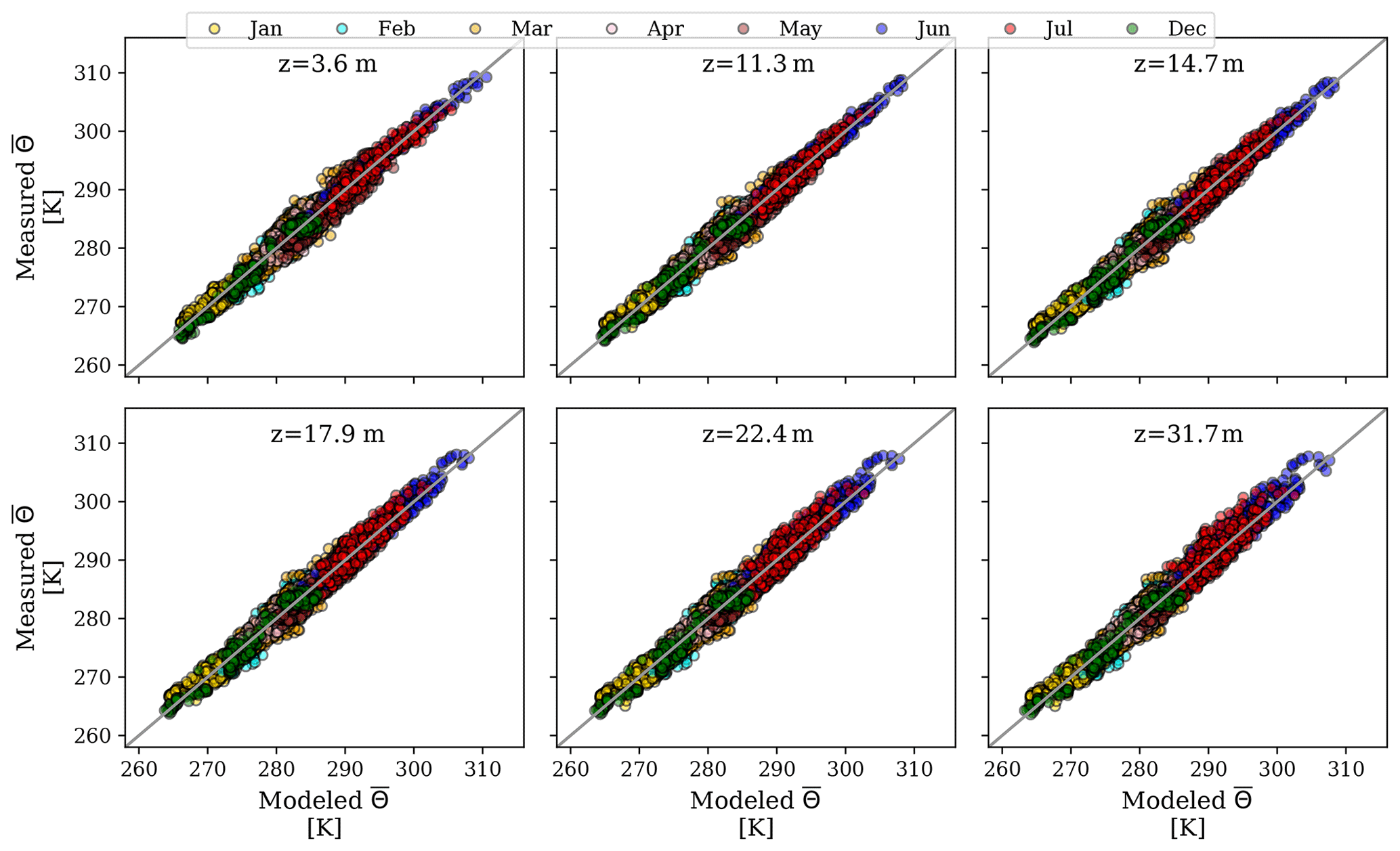
Figure 3 Scatter plots of observed (BUBBLE) versus simulated (VCWG) values of potential temperature for different altitudes and months; each data point corresponds to a 1 h comparison between the model and observation.

Table 2 Bias (K), RMSE (K), and R² (–) for VCWG predictions of potential temperature against the BUBBLE observations for different altitudes and months.

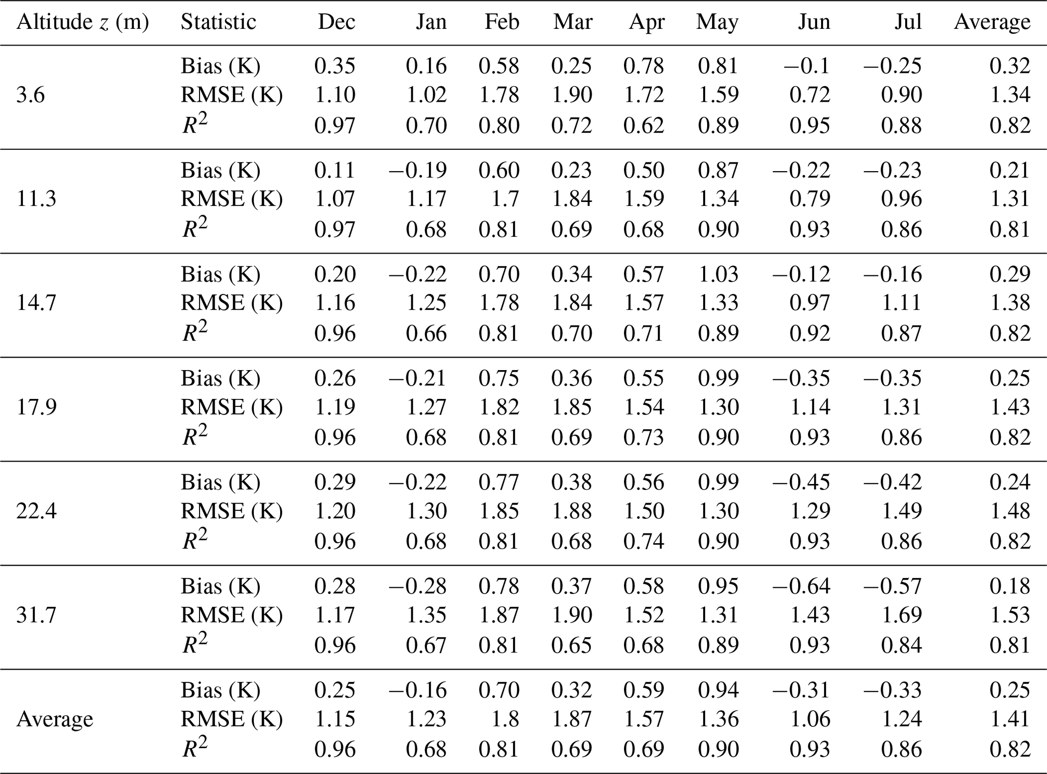
Figure 4 shows the diurnal variation of the observed versus simulated values of potential temperature averaged for every hour of the day for the available months. The diurnal patterns in temperature reveal that the model has similar skill in predicting the potential temperature during all hours at lower elevations (z=3.6 to 14.7 m). This performance is comparable to other models that show a well-captured diurnal variation of potential temperature at low altitudes (Bueno et al., 2012a; Krayenhoff et al., 2020; Meili et al., 2020; Mussetti et al., 2020). However, the diurnal pattern in temperature can deviate between the model and observations at higher elevations (z=17.9 to 31.7 m), especially during midday hours. This can be attributed to more complex flow patterns in the above-roof-level space due to heat advection, horizontal heterogeneity of the urban site, and the above-roof-level shear layer.

Figure 4 Comparison between the observed (BUBBLE) versus simulated (VCWG) values of potential temperature. The hourly means are shown, and nighttime is indicated by shaded regions. Solid line: model, dashed line: observation. Times are in local standard time (LST).

3.1.3 Wind speed

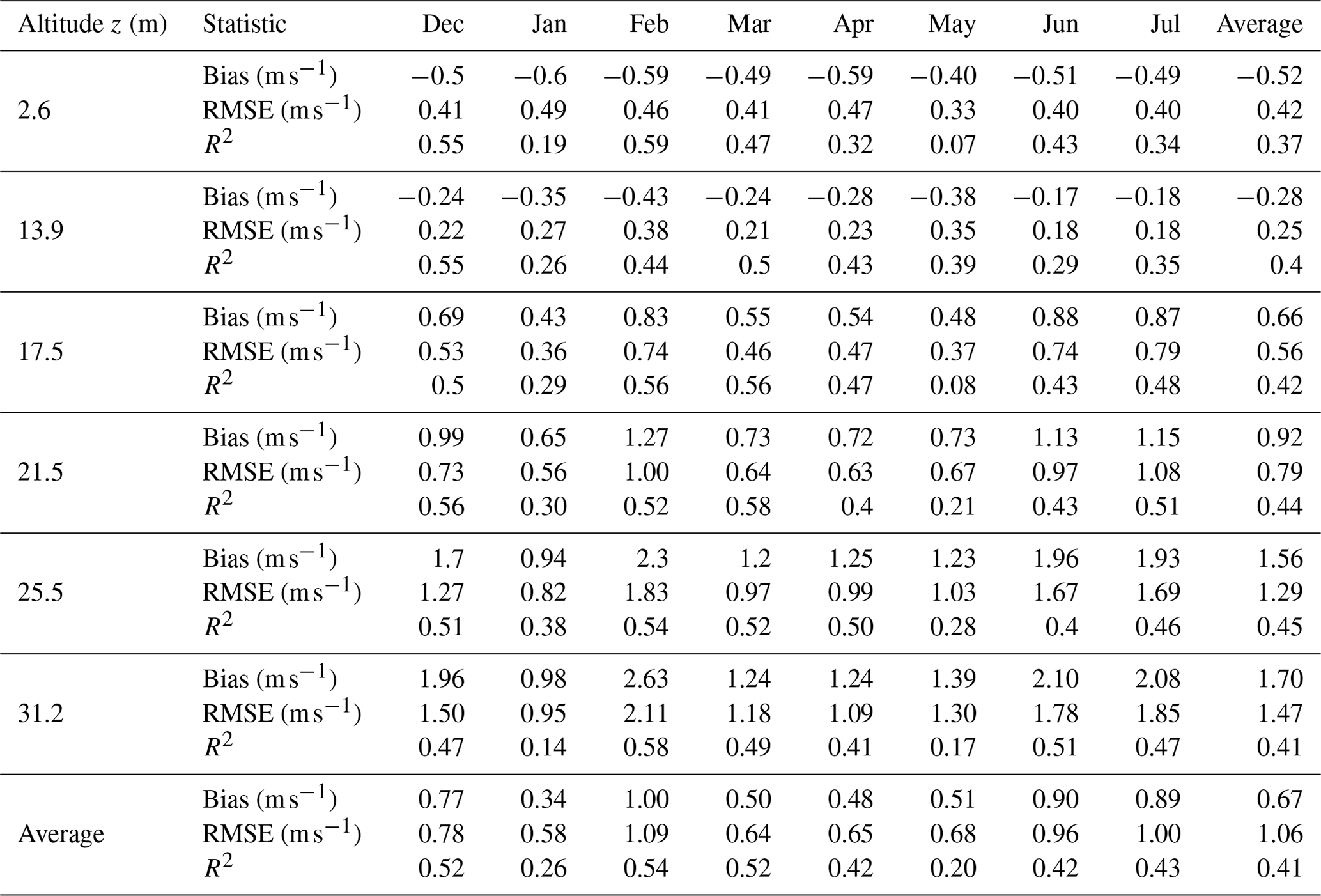
Figure 5 and Table 3 show scatter plots of the observed versus simulated values of wind speed and the statistical metrics used for the comparison. Considering all altitudes and months, the average bias, RMSE, and R² are 0.67 m s⁻¹, 1.06 m s⁻¹, and 0.41, respectively. Although the comparison reveals a reasonable bias and RMSE, the R² is lower than values reported for comparisons of potential temperature and specific humidity. This can be explained by the fact that the urban morphology is highly heterogeneous, the measurement of wind is location-specific, and the wind speed and direction can change considerably within each hour. Heterogeneous urban morphology results in great spatial variability of the components of wind velocity vector as a function of wind direction and wind speed (Klein and Clark, 2007; Klein and Galvez, 2015; Afshari and Ramirez, 2021). On the other hand, forced by hourly rural measurements, VCWG assumes a regular urban morphology and predicts the volume-averaged horizontal wind velocity components. So it is expected to obtain lower R² values. Other models also often report lower R² values for wind speed compared to potential temperature and specific humidity (Mussetti et al., 2020). Overall, our bias, RMSE, and R² values are in agreement with values reported in the literature. For instance, Lemonsu et al. (2012) reported a range in bias of −0.16 to 0.56 m s⁻¹. They also reported a range in RMSE of 0.40 to 0.69 m s⁻¹. Mussetti et al. (2020) reported a bias, RMSE, and R² of 0.61 m s⁻¹, 1.31 m s⁻¹, and 0.70 , respectively.

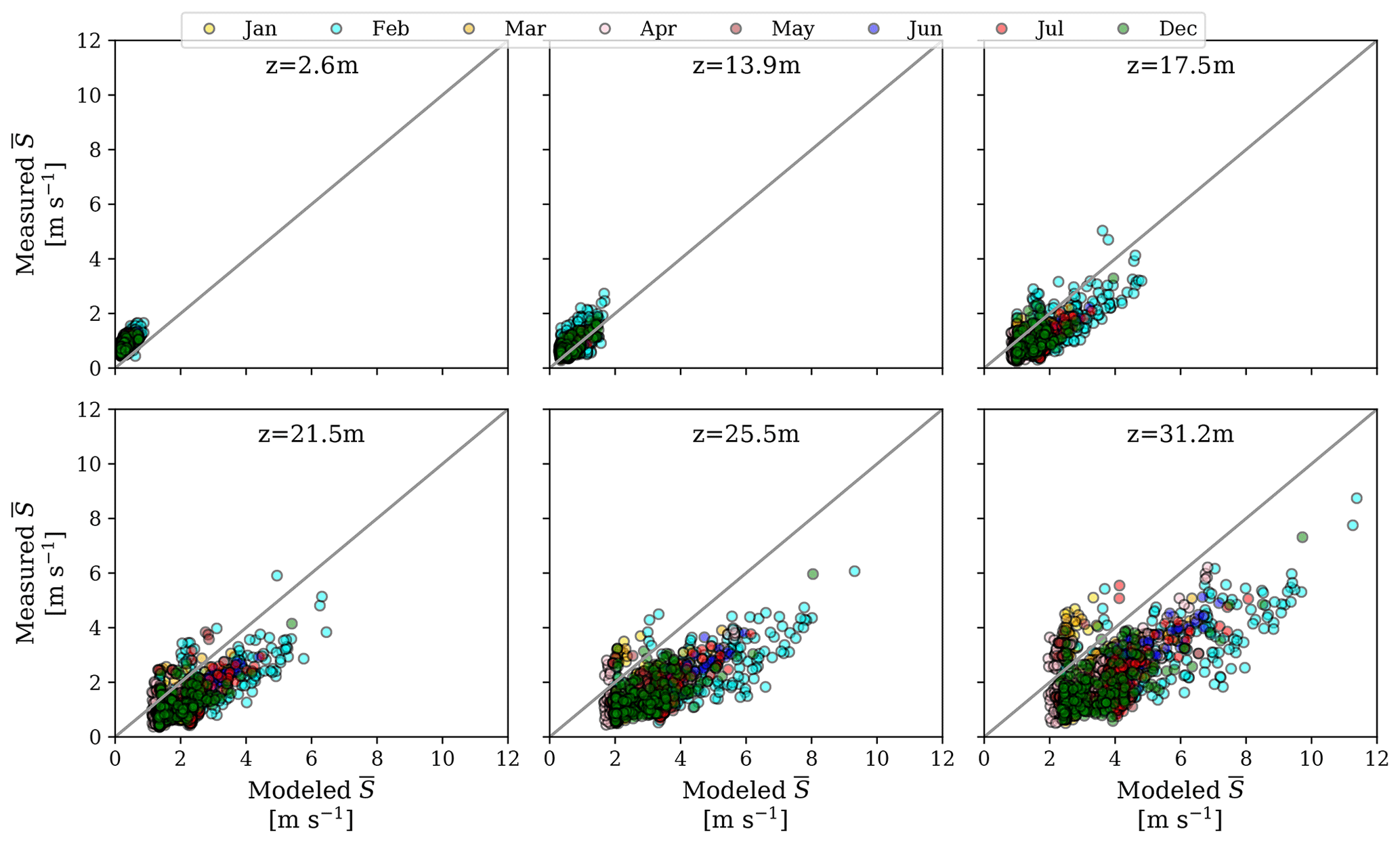
Figure 5 Scatter plots of observed (BUBBLE) versus simulated (VCWG) values of wind speed for different altitudes and months; each data point corresponds to a 1 h comparison between the model and observation.

Table 3 Bias (m s⁻¹), RMSE (m s⁻¹), and R² (–) for VCWG predictions of wind speed against the BUBBLE observations for different altitudes and months.

3.1.4 Specific humidity

Figure 6 and Table 4 show scatter plots of the observed versus simulated values of specific humidity and the statistical metrics used for the comparison. Note that specific humidity data were only available in June–July 2002. Over all altitudes and the available months, on average, the bias, RMSE, and R² for specific humidity are 0.00057 kg kg⁻¹, 0.0010 kg kg⁻¹, and 0.85, respectively. These statistics are comparable to what has been reported in the literature for similar models that were compared against observations. For instance, Mussetti et al. (2020) reported a bias, RMSE, and R² of −0.00109 kg kg⁻¹, 0.00152 kg kg⁻¹, and 0.74, respectively, above the urban canopy for comparisons of a model and observations in summer. Lemonsu et al. (2012) reported a range in bias of −0.00116 to −0.0005 kg kg⁻¹. They also reported a range in RMSE of 0.00081 to 0.00172 kg kg⁻¹.

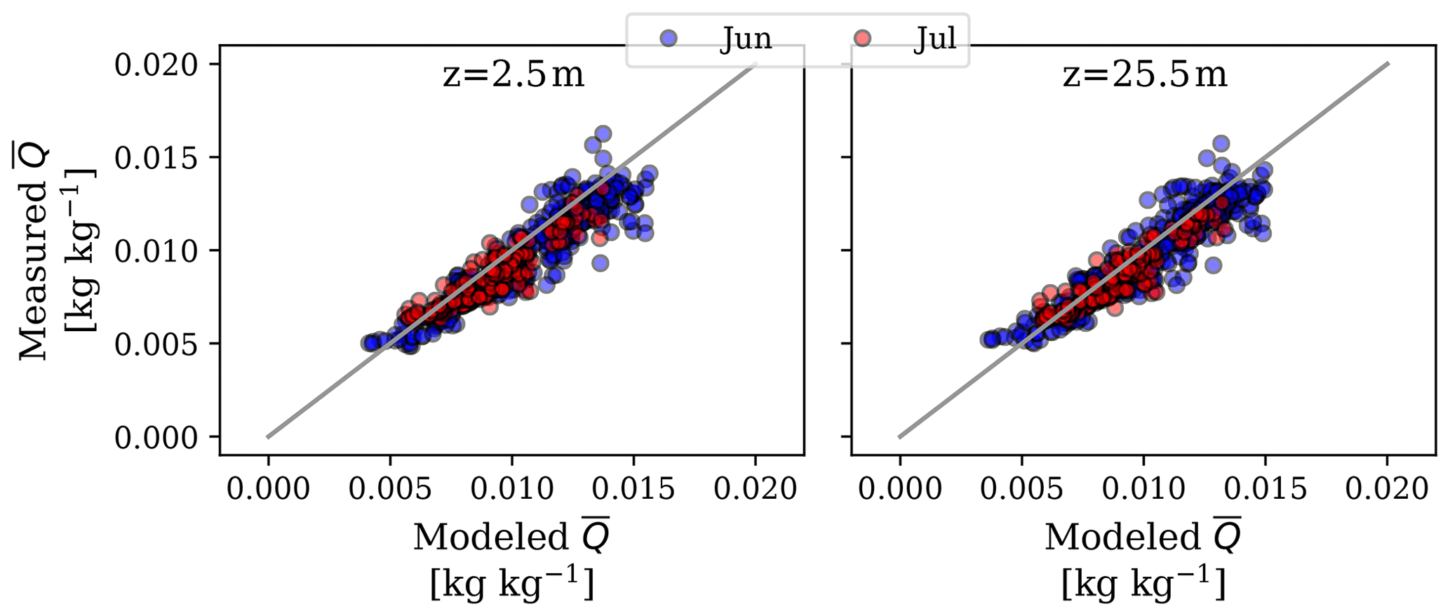
Figure 6 Scatter plots of observed (BUBBLE) versus simulated (VCWG) values of specific humidity for different altitudes and months; each data point corresponds to a 1 h comparison between the model and observation.

Table 4 Bias (kg kg⁻¹), RMSE (kg kg⁻¹), and R² (–) for VCWG predictions of specific humidity against the BUBBLE observations for different altitudes and months.

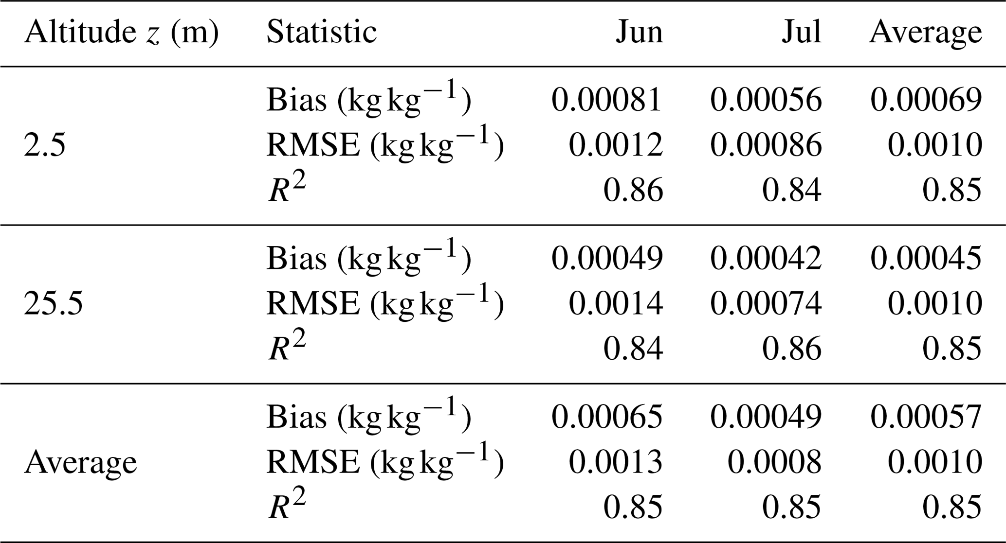
Figure 7 shows the diurnal variation of the observed versus simulated values of specific humidity averaged for every hour of the day for June–July 2002. While the diurnal variation is predicted by the model, some deviations are noted between the model and the observation. The model overpredicts the values at night, while it underpredicts the values during midday, especially at z=25.5 m. This could be due to the assumptions of the rural model to generate the vertical profile of specific humidity. In this model the latent heat flux in the rural area is parameterized as a function of the sensible heat flux and a fixed Bowen ratio. However, the Bowen ratio can vary diurnally (Kalanda et al., 1979). This can result in a slight miscalculation of the latent heat flux and a forcing boundary condition for specific humidity on top of the modeling domain.

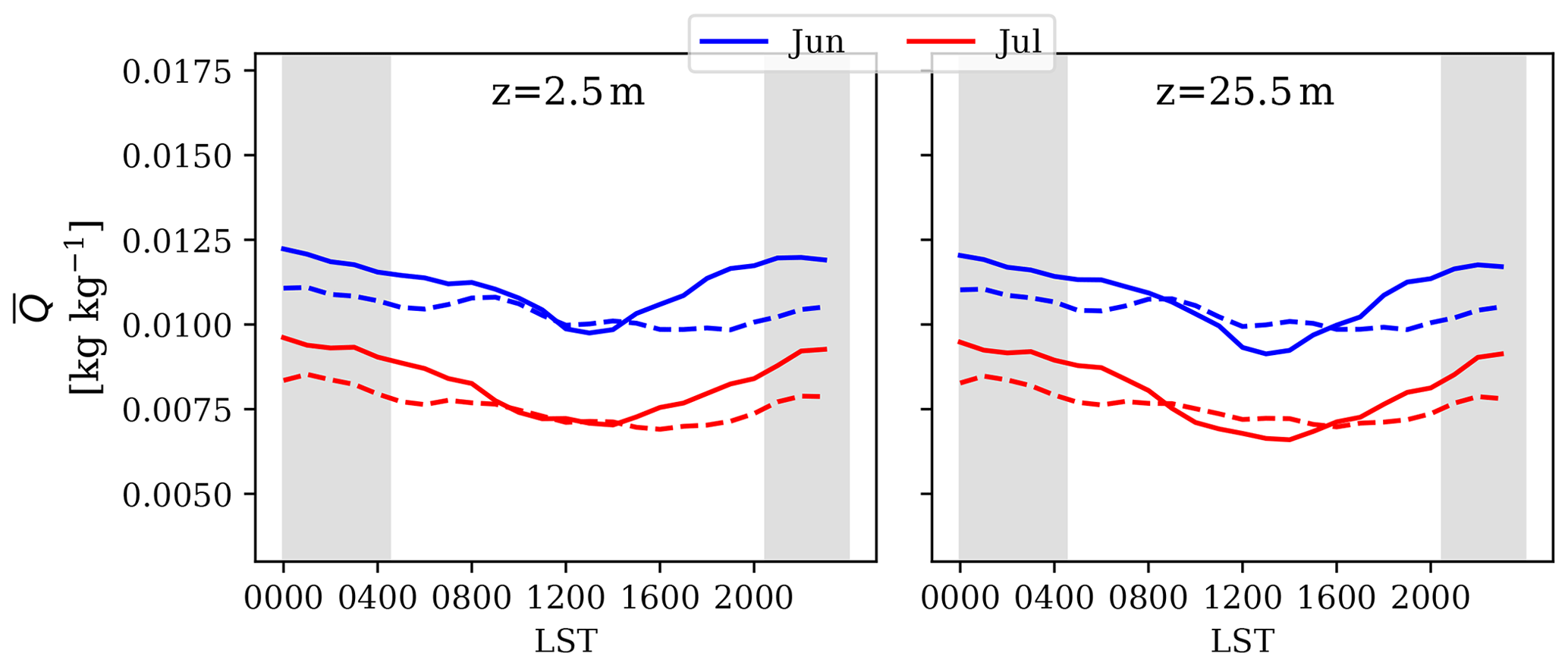
Figure 7 Comparison between the observed (BUBBLE) versus simulated (VCWG) values of specific humidity. The hourly means are shown, and nighttime is indicated by shaded regions. Solid line: model, dashed line: observation. Times are in local standard time (LST).

3.1.5 Urban heat island (UHI)

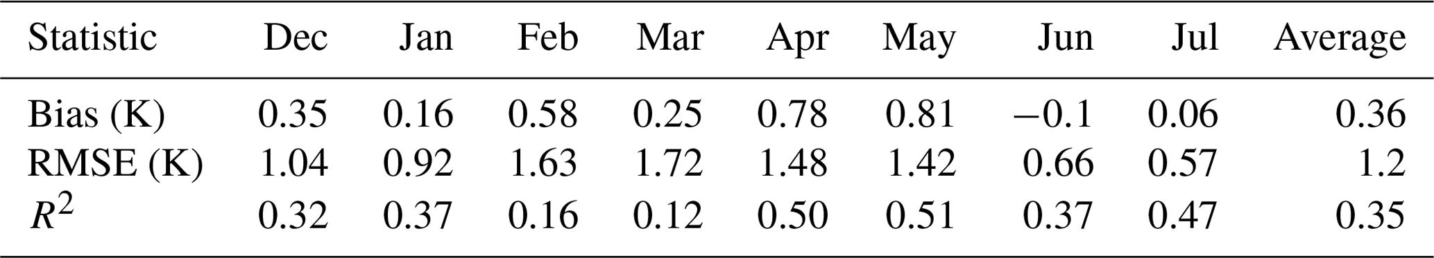
To compare VCWG results with measured UHI (K) from the BUBBLE campaign, the bias, RMSE, and R² are computed for pairs of hourly model versus observed values for the available months. UHI (K) for the observation is computed by considering the difference between the temperature measurements inside the canyon at z=3.6 m and temperatures provided by the EPW dataset. For VCWG, UHI (K) is calculated by considering the difference between the temperature prediction inside the canyon at z=3 m and temperatures provided by the EPW dataset. Figure 8 and Table 5 show the diurnal variation of UHI (for both observations and simulations) and the statistical metrics used for the comparison. On average, the bias, RMSE, and R² for UHI (K) are 0.36 K, 1.2 K, and 0.35, respectively. VCWG predictions of UHI (K) are more successful for the months of December, January, April, May, June, and July (R²>0.3) than for the months of February and March (R²<0.2). The deviations in predicting UHI (K) may be attributed to several factors. The heterogeneity of the urban environment and placement of urban sensors may result in sensing slightly warmer or colder temperatures than the spatial average due to the spatial variability of temperature (Mussetti et al., 2020). Also, the relative position of the rural site with respect to the urban site, variation of dominant wind directions over different seasons, and horizontal advective transport of heat from the rural area may confound the prediction of UHI. Given that VCWG does not consider all such variations due to simplifying assumptions, it is expected to predict different values of UHI (K) over different seasons in comparison to observations. Nevertheless, overall, the statistics for UHI (K) comparison are in reasonable agreement with those reported by other models. For example, Mussetti et al. (2020) reported bias, RMSE, and R² values of −1.88 K, 1.66 K, and 0.55, respectively, for near-ground predictions of UHI (K) in the summer.

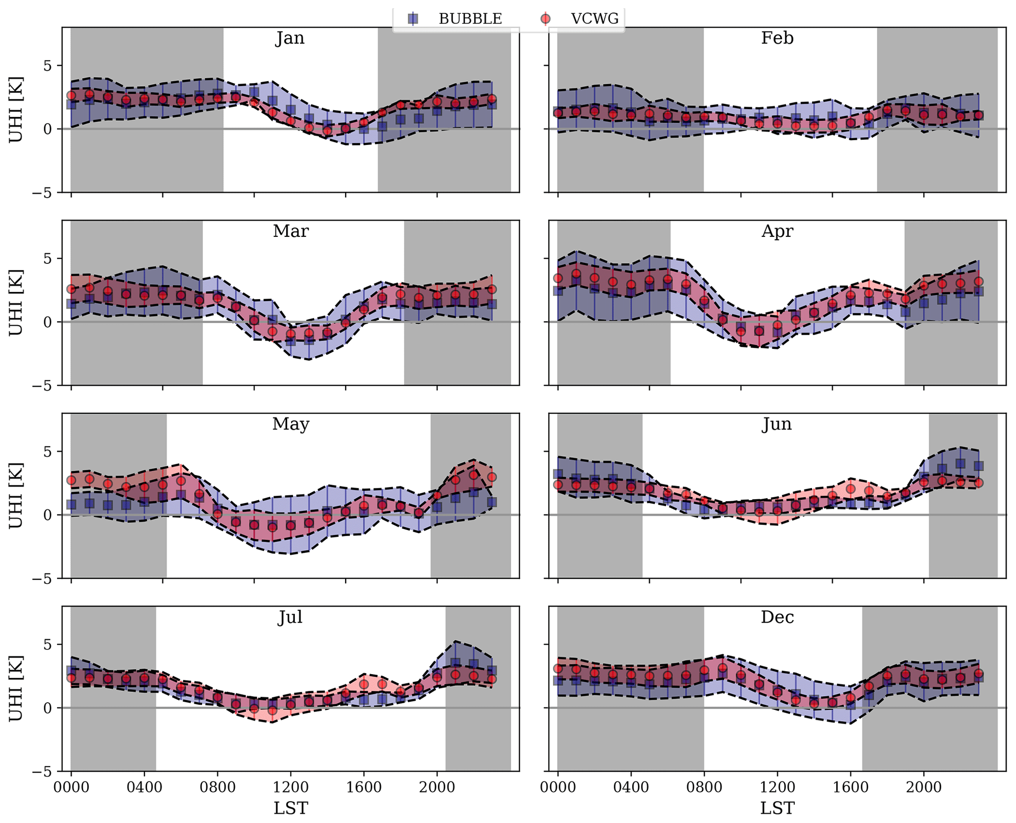
Figure 8 Hourly mean and standard deviation (band) of UHI (K) in each month for the observed (BUBBLE) and predicted (VCWG) values; nighttime is indicated by shaded regions. Times are in local standard time (LST).

Table 5 Bias (K), RMSE (K), and R² (–) for VCWG predictions of UHI (K) against the BUBBLE observations for different months.

3.2 Model exploration and comparison with limited UHI observations

In this section we explore the capability of the VCWG model to predict urban climate for investigations of the effects of building dimensions, urban vegetation, building energy configuration, radiation configuration, seasonal variations, and other climates. These results are reported in the Supplement in detail. Here only brief references to the analysis are made. Many explorations consider both nighttime and daytime urban microclimate. First, we investigate how the urban geometry, which is characterized by plan area density λ_p (–) and frontal area density λ_f (–), can affect the urban microclimate. An increase in λ_p from 0.46 to 0.54 (–) is associated with lower air temperatures (due to shading) and reduces wind speed within the urban canyon during daytime (see Fig. S1 in the Supplement). An increase in λ_f from 0.37 to 0.51 (–) also increases shading effects and consequently reduces daytime temperatures, but it increases nighttime temperatures due to more heat released from urban surfaces that is trapped in the canyon (see Fig. S2 in the Supplement). The cooling effect of urban vegetation is also evaluated by changing the leaf area density (LAD; m²m⁻³) profiles within the canyon. Increasing the average LAD from 0.1 to 0.2 (m²m⁻³) shows heat removal from the canyon alongside lower wind speed due to the drag induced by trees (see Fig. S3 in the Supplement). VCWG simulations are also conducted for different building types (a mid-rise apartment and a hospital), cooling system coefficients of performance (–), heating thermal efficiencies η_heat (–), and locations of building waste heat release F_st (–). The results show that a hospital generates more waste heat fluxes associated with cooling and gas consumption, which increase urban temperatures (see Fig. S4 in the Supplement). The analysis of different cooling and heating systems also reveals that less efficient systems (lower COP from 3.13 to 1 (–) and η_heat from 0.8 to 0.4; –) result in more waste heat emission and slightly higher temperatures (see Fig. S5 in the Supplement). It is found that releasing building waste heat at street level contributes to a higher UHI (K), by 1 K, than releasing the waste heat at roof level (see Fig. S6 in the Supplement). This can be due to more effective heat removal from the urban roughness sublayer when the heat is released at roof level. The radiation model is assessed by VCWG simulations for different canyon aspect ratios and axis angles. The radiation fluxes at the road and walls show differences according to canyon aspect ratio and axis angle, while the fluxes at the tree canopy and roof are less sensitive to the canyon aspect ratio and axis angle (see Figs. S7 and S8). The performance of VCWG is assessed over different seasons with simulations for Vancouver for an entire year. It is found that early daytime UHI (K) values are lower than nighttime values, as expected. Also, the greatest UHI (K) values are predicted to occur in August and September (see Fig. S9 in the Supplement). Seasonal variations of the vertical profiles of potential temperature, wind speed, specific humidity, and turbulent kinetic energy reveal that the seasonal variations in potential temperature and specific humidity are higher than those associated with wind speed and turbulent kinetic energy (see Fig. S10 in the Supplement). Finally, the ability of the model to predict UHI (K) in different cities with different climate zones is assessed. The case studies are Buenos Aires, Vancouver, Osaka, and Copenhagen (see Fig. S11 in the Supplement). All exploration results obtained from the VCWG are reasonably consistent with previous observations in the literature.

4 Conclusions and future work

The Vertical City Weather Generator (VCWG) is an urban microclimate model designed to calculate vertical profiles of meteorological variables including potential temperature, wind speed, specific humidity, and turbulent kinetic energy in an urban area. The VCWG is composed of four sub-models for ingestion of urban parameters and meteorological variables in a rural area (as input and boundary conditions) as well as prediction of the meteorological variables in a nearby urban area, the building energy performance variables, and the shortwave and longwave radiation transfer processes. VCWG combines elements of several previous models developed by Santiago and Martilli (2010), Bueno et al. (2014), Krayenhoff (2014), Krayenhoff et al. (2015), and Meili et al. (2020) to generate a model with the ability to predict vertical profiles of urban meteorological variables forced by rural measurements with two-way coupling to both building energy and radiation models.

To evaluate VCWG, its predictions of potential temperature, wind speed, and specific humidity are compared to observations from the Basel UrBan Boundary Layer Experiment (BUBBLE) microclimate field campaign for 8 months from December 2001 to July 2002 (Christen and Vogt, 2004; Rotach et al., 2005). The model evaluation indicates that the VCWG predicts vertical profiles of meteorological variables in reasonable agreement with field measurements. The average bias, RMSE, and R² for potential temperature are 0.25 K, 1.41 K, and 0.82, respectively. The average bias, RMSE, and R² for wind speed are 0.67 m s⁻¹, 1.06 m s⁻¹, and 0.41, respectively. The average bias, RMSE, and R² for specific humidity are 0.00057 kg kg⁻¹, 0.0010 kg kg⁻¹, and 0.85, respectively. In addition, the average bias, RMSE, and R² for the urban heat island (UHI) are 0.36 K, 1.2 K, and 0.35, respectively. Based on the evaluations, the model performance is comparable to the performance of similar models. The performance of the model is further explored to investigate the effects of urban configurations such as plan and frontal area densities, varying levels of vegetation, building energy configuration, radiation configuration, seasonal variations, and different climate zones on the model predictions. The exploration results also show acceptable performance in agreement with known urban physical processes and observations.

This study shows that the urban microclimate model VCWG can successfully extend the spatial dimension of preexisting bulk flow (single-layer) urban microclimate models to one dimension in the vertical direction, while it also considers the relationship of the urban microclimate model to the rural meteorological measurements and the building energy conditions. The effect of the key urban elements such as building configuration, building energy systems (e.g., location of condensers and exhaust stacks), surface vegetation, and trees are considered, but there is still opportunity to improve VCWG further. The urban site is simplified as blocks of buildings with symmetric and regular dimensions, which can be more realistically represented if more considerations are taken into account regarding the nonuniform distribution of building dimensions. Also, the building energy model in VCWG is a single-zone model, assuming a uniform temperature with height in both indoor and outdoor environments. This limitation can be overcome by improving the radiation model, urban vertical diffusion model, and building energy model so that wall and indoor temperatures can vary with height, allowing the development of a multi-zone building energy model. In addition, horizontal advection from the rural area can be considered and parameterized in future work. Future studies can also focus on an improvement of the flow-field parameterization or include additional source and sink terms in the transport equations to model horizontal motions, eddies, and flow fluctuations in the urban area, which is realistically very three-dimensional and heterogeneous. Urban hydrology can be added to VCWG in the future to account for precipitation effects. At present, the developed VCWG model can account for the spatial variation of urban microclimate in a computationally efficient manner independent of an auxiliary mesoscale model. This advantage is really important for urban planners, architects, and consulting engineers for operationally fast VCWG simulations.

Appendix A

A1 Surface energy balance in the rural area

In Eq. (7) the net shortwave solar radiation flux absorbed at the surface can be calculated from

$$\begin{array}{ll}\text{(A1)}& {\displaystyle }{Q}_{\mathrm{S},\text{rur}}=& {\displaystyle }\left(\right(\mathrm{1}-F_{\text{veg}}\left)\right(\mathrm{1}-{\mathit{\alpha }}_{\text{rur}})+F_{\text{veg}}(\mathrm{1}-{\mathit{\alpha }}_{\mathrm{V}}\left)\right){\displaystyle }& {\displaystyle }\cdot (S^{\downarrow \text{direct}}+S^{\downarrow \text{diffuse}}),\end{array}$$

where F_veg (–) is the fraction of the rural area covered by vegetation, α_rur (–) is overall albedo of the rural area, α_V (–) is the albedo of vegetation (here considered to be the same for rural and urban vegetation), and S^↓direct and S^↓diffuse (W m⁻²) are the forcing direct and diffuse shortwave radiation fluxes from the EPW file, respectively. The net longwave radiation flux absorbed at the surface can be calculated from

$$\begin{array}{}\text{(A2)}& Q_{\mathrm{L},\text{rur}}=L^{\downarrow }-L^{\uparrow }={\mathit{\epsilon }}_{\text{rur}}\left(L^{\downarrow }-\mathit{\sigma }{T}_{\mathrm{s},\text{rur}}^{\mathrm{4}}\right),\end{array}$$

where L^↓ (W m⁻²) is the forcing longwave radiation flux from the EPW file, L^↑ (W m⁻²) is the longwave radiation flux leaving the rural surface at temperature T_s,rur (K), and ε_rur (–) is rural surface emissivity. The net sensible heat flux is calculated using Louis (1979):

$$\begin{array}{ll}\text{(A3)}& {\displaystyle }{Q}_{\text{sen},\text{rur}}=& {\displaystyle }-\mathit{\rho }{C}_{\mathrm{p}}{\displaystyle \frac{{\mathit{\kappa }}^{\mathrm{2}}}{{\left(\ln \frac{z}{z_{{\mathrm{0}}_{\text{rur}}}}\right)}^{\mathrm{2}}}}{\displaystyle \frac{\mathrm{1}}{R}}{\stackrel{\mathrm{‾}}{S}}_{\text{rur},z=\mathrm{10}m}{\displaystyle }& {\displaystyle }\cdot \left({\stackrel{\mathrm{‾}}{\mathrm{\Theta }}}_{\text{rur},\mathrm{2}m}-{\stackrel{\mathrm{‾}}{\mathrm{\Theta }}}_{\text{rur},\mathrm{s}}\right)F_{\mathrm{h}}\left({\displaystyle \frac{z}{z_{{\mathrm{0}}_{\text{rur}}}}},{\mathit{\text{Ri}}}_{\mathrm{B}}\right),\end{array}$$

where R (–) is a model constant, Ri_B (–) is the bulk Richardson number, and F_h (–) is the stability function for sensible heat flux defined by Louis (1979). The net latent heat flux is calculated using the Bowen ratio β_rur (–) such that $Q_{\text{lat},\text{rur}}=Q_{\text{sen},\text{rur}}/{\mathit{\beta }}_{\text{rur}}$ (W m⁻²). The ground heat flux drives the conduction equation at the uppermost soil layer via Bueno et al. (2012a):

$$\begin{array}{}\text{(A4)}& d{C}_{\mathrm{v}}{\displaystyle \frac{\mathrm{d}{T}_{\mathrm{1}}}{\mathrm{d}t}}=C(T_{\mathrm{2}}-T_{\mathrm{1}})+Q_{\text{grd}},\end{array}$$

where d (m) is the soil layer thickness, C_v ($\mathrm{J}{\mathrm{m}}^{-\mathrm{3}}{\mathrm{K}}^{-\mathrm{1}}$) is volumetric heat capacity of soil, $T_{\mathrm{1}}={\stackrel{\mathrm{‾}}{\mathrm{\Theta }}}_{\text{rur},\mathrm{s}}$ (K) is soil upper layer temperature (the same as soil surface temperature), C (${\mathrm{Wm}}^{-\mathrm{2}}{\mathrm{K}}^{-\mathrm{1}}$) is the soil thermal conductance, and T₂ (K) is soil temperature in the second layer underground. In the lowest layer (n) of soil the conduction equation is forced by a deep soil temperature T_deep (K):

$$\begin{array}{}\text{(A5)}& d{C}_{\mathrm{v}}{\displaystyle \frac{\mathrm{d}{T}_{n-\mathrm{1}}}{\mathrm{d}t}}=C(T_{\text{deep}}-T_{n-\mathrm{1}}).\end{array}$$

A2 Source and sink term in the 1D model

The pressure and skin drags exerted on the flow in Eqs. (8) and (9) are formulated as follows (Santiago and Martilli, 2010; Krayenhoff, 2014; Krayenhoff et al., 2015, 2020; Simón-Moral et al., 2017; Nazarian et al., 2020):

$$\begin{array}{}\text{(A6)}& {\displaystyle }& {\displaystyle }{D}_x=\underset{\mathrm{I}}{\underbrace{{\displaystyle \frac{\mathrm{1}}{\mathit{\rho }}}{\displaystyle \frac{\partial \stackrel{\mathrm{̃}}{P}}{\partial x}}}}+\underset{\text{II}}{\underbrace{\mathit{\nu }\left({\mathrm{\nabla }}^{\mathrm{2}}\stackrel{\mathrm{̃}}{U}\right)}},\text{(A7)}& {\displaystyle }& {\displaystyle }{D}_y=\underset{\mathrm{I}}{\underbrace{{\displaystyle \frac{\mathrm{1}}{\mathit{\rho }}}{\displaystyle \frac{\partial \stackrel{\mathrm{̃}}{P}}{\partial y}}}}+\underset{\text{II}}{\underbrace{\mathit{\nu }\left({\mathrm{\nabla }}^{\mathrm{2}}\stackrel{\mathrm{̃}}{V}\right)}},\end{array}$$

where term I represents a dispersive pressure variation (form drag) induced by vegetation and building, and term II represents the dispersive viscous dissipation (skin drag) induced by horizontal surfaces. The former can be parameterized as

$$\begin{array}{}\text{(A8)}& {\displaystyle }& {\displaystyle \frac{\mathrm{1}}{\mathit{\rho }}}{\displaystyle \frac{\partial \stackrel{\mathrm{̃}}{P}}{\partial x}}=\left(B_{\mathrm{D}}{C}_{\text{DBv}}+\text{LAD}\mathrm{\Omega }{C}_{\text{DV}}\right){\stackrel{\mathrm{‾}}{U}}_{\text{expl}}\stackrel{\mathrm{‾}}{U},\text{(A9)}& {\displaystyle }& {\displaystyle \frac{\mathrm{1}}{\mathit{\rho }}}{\displaystyle \frac{\partial \stackrel{\mathrm{̃}}{P}}{\partial y}}=\left(B_{\mathrm{D}}{C}_{\text{DBv}}+\text{LAD}\mathrm{\Omega }{C}_{\text{DV}}\right){\stackrel{\mathrm{‾}}{V}}_{\text{expl}}\stackrel{\mathrm{‾}}{V},\end{array}$$

where B_D (m⁻¹) is the sectional building area density, C_DBv (–) is the sectional drag coefficient in the presence of trees, LAD (m²m⁻³) is leaf area density in the canyon, Ω (–) is a clumping factor, C_DV (–) is the drag coefficient for tree foliage, and ${\stackrel{\mathrm{‾}}{U}}_{\text{expl}}$ and ${\stackrel{\mathrm{‾}}{V}}_{\text{expl}}$ (m s⁻¹) are wind velocity components in the x and y directions from a previous numerical solution, respectively, which are explicitly assumed to be constants to linearize the system of equations to be solved. The skin drag can be parameterized as follows:

$$\begin{array}{}\text{(A10)}& {\displaystyle }& {\displaystyle }\mathit{\nu }\left({\mathrm{\nabla }}^{\mathrm{2}}\stackrel{\mathrm{̃}}{U}\right)={\displaystyle \frac{\mathrm{1}}{\mathrm{\Delta }z}}{c}_{\mathrm{d}}{f}_{\mathrm{m}}{\stackrel{\mathrm{‾}}{U}}_{\text{expl}}\stackrel{\mathrm{‾}}{U},\text{(A11)}& {\displaystyle }& {\displaystyle }\mathit{\nu }\left({\mathrm{\nabla }}^{\mathrm{2}}\stackrel{\mathrm{̃}}{V}\right)={\displaystyle \frac{\mathrm{1}}{\mathrm{\Delta }z}}{c}_{\mathrm{d}}{f}_{\mathrm{m}}{\stackrel{\mathrm{‾}}{V}}_{\text{expl}}\stackrel{\mathrm{‾}}{V},\end{array}$$

where c_d (–) is skin drag coefficient and f_m (–) is a function of stability from Louis (1979). The terms related to the wake production S_wake and dissipation rate ε (both in m²s⁻³) in Eq. (11) can be parameterized as

$$\begin{array}{}\text{(A12)}& {\displaystyle }& {\displaystyle }{S}_{\text{wake}}=\left(B_{\mathrm{D}}{C}_{\text{DBv}}+\text{LAD}\mathrm{\Omega }{C}_{\text{DV}}\right){\stackrel{\mathrm{‾}}{U}}_{\text{expl}}^{\mathrm{3}},\text{(A13)}& {\displaystyle }& {\displaystyle }\mathit{\epsilon }=C_{\mathit{\epsilon }}{\displaystyle \frac{k^{\frac{\mathrm{3}}{\mathrm{2}}}}{{\mathrm{\ell }}_{\mathit{\epsilon },\text{dissip}}}},\end{array}$$

where Ω (–) is a clumping factor, C_ε (–) is a model constant, and ℓ_ε,dissip (m) is a dissipation length scale obtained through a sensitivity study using CFD (Nazarian et al., 2020). Note that plan area density λ_p (–) in this study is greater than the limit considered by Nazarian et al. (2020), so we assume that the parameterizations extrapolate to this value of λ_p (–). The heat source and sink terms, which are the terms in Eq. (12), caused by the roof (S_ΘR) and ground (S_ΘG) (both in K s⁻¹) are calculated based on the study by Louis (1979) and the heat flux from the wall (S_ΘW; K s⁻¹) is formulated in Martilli et al. (2002). The two other source and sink terms can be parameterized as follows:

$$\begin{array}{}\text{(A14)}& {\displaystyle }& {\displaystyle }{S}_{\mathrm{\Theta }\mathrm{A}}={\displaystyle \frac{\mathrm{4}{\mathit{\rho }}_{\text{abs}}{k}_{\text{air}}}{\mathit{\rho }{C}_{\mathrm{p}}{v}_{\mathrm{L}}}}\left[(\mathrm{1}-{\mathit{\lambda }}_{\mathrm{p}})L_{\mathrm{A}}\right],\text{(A15)}& {\displaystyle }& {\displaystyle }{S}_{\mathrm{\Theta }\mathrm{V}}={\displaystyle \frac{\mathrm{2}{g}_{\text{Ha}}{c}_{\text{PM}}}{\mathit{\rho }{C}_{\mathrm{p}}{v}_{\mathrm{L}}}}\left[\text{LAD}(\mathrm{1}-{\mathit{\lambda }}_{\mathrm{p}})({\stackrel{\mathrm{‾}}{\mathrm{\Theta }}}_{\mathrm{V}}-\stackrel{\mathrm{‾}}{\mathrm{\Theta }})\right],\end{array}$$

where L_A (W m⁻²) is the absorbed flux density of longwave radiation in the canyon, ρ_abs (kg m⁻³) is the density of absorbing molecules, k_air (m² kg⁻¹) is their mass extinction cross section, $v_{\mathrm{L}}=(\mathrm{1}-{\mathit{\lambda }}_{\mathrm{p}})$ (–) is the fraction of total volume that is outdoor air, g_Ha ($\mathrm{mol}{\mathrm{m}}^{-\mathrm{2}}{\mathrm{s}}^{-\mathrm{1}}$) is conductance for heat, c_PM ($\mathrm{J}{\mathrm{mol}}^{-\mathrm{1}}{\mathrm{K}}^{-\mathrm{1}}$) is the molar heat capacity for the air, and ${\stackrel{\mathrm{‾}}{\mathrm{\Theta }}}_{\mathrm{V}}$ (K) is the potential temperature of tree foliage. In the specific humidity equation, Eq. (16), the source and sink term can be calculated using the following equation:

$$\begin{array}{}\text{(A16)}& S_{\text{QV}}={\displaystyle \frac{{\mathrm{\Lambda }}_{\mathrm{M}}{g}_{\mathrm{v}}\mathrm{\Omega }}{\mathit{\rho }\mathrm{\Lambda }{v}_{\mathrm{L}}}}\left[\text{LAD}(\mathrm{1}-{\mathit{\lambda }}_{\mathrm{p}})\left(s[{\stackrel{\mathrm{‾}}{\mathrm{\Theta }}}_{\mathrm{V}}-\stackrel{\mathrm{‾}}{\mathrm{\Theta }}]+{\displaystyle \frac{D}{P}}\right)\right],\end{array}$$

where Λ_M (J mol⁻¹) is the molar latent heat of vaporization, Λ (J kg⁻¹) is the latent heat of vaporization, g_v ($\mathrm{mol}{\mathrm{m}}^{-\mathrm{2}}{\mathrm{s}}^{-\mathrm{1}}$) is the average surface and boundary layer conductance for humidity for the whole leaf, s (K⁻¹) is a derivative of saturation vapor pressure with respect to temperature divided by pressure, D (Pa) is the vapor deficit of the atmosphere, and P (Pa) is atmospheric pressure.

A3 Building heat exchanges

The heat fluxes in Eq. (17) can be parameterized as

$$\begin{array}{}\text{(A17)}& {\displaystyle }& {\displaystyle }{Q}_{\text{surf}}=\mathrm{\Sigma }{h}_i{A}_i|T_{\text{si}}-T_{\text{in}}|,\text{(A18)}& {\displaystyle }& {\displaystyle }{Q}_{\text{inf}}={\dot{m}}_{\text{inf}}{C}_{\mathrm{p}}|T_{\text{out}}-T_{\text{in}}|,\text{(A19)}& {\displaystyle }& {\displaystyle }{Q}_{\text{vent}}={\dot{m}}_{\text{vent}}{C}_{\mathrm{p}}|T_{\text{supp}}-T_{\text{in}}|,\end{array}$$

where h_i ($\mathrm{W}{\mathrm{m}}^{-\mathrm{2}}{\mathrm{K}}^{-\mathrm{1}}$) is the convective heat transfer coefficient for surface i, and A_i (m² m⁻²) is the surface area for surface i per building footprint area. Surface i can correspond to indoor elements such as ceiling, walls, floor, building mass, and windows. T_si (K) is the temperature of the inner layer of elements, T_in (K) is indoor temperature, T_out (K) is the outdoor temperature averaged over building height, T_supp (K) is supply temperature, ${\dot{m}}_{\text{inf}}$ ($\mathrm{kg}{\mathrm{s}}^{-\mathrm{1}}{\mathrm{m}}^{-\mathrm{2}}$) is the mass flow rate of infiltration (exfiltration) per building footprint area, and ${\dot{m}}_{\text{vent}}$ ($\mathrm{kg}{\mathrm{s}}^{-\mathrm{1}}{\mathrm{m}}^{-\mathrm{2}}$) is mass flow rate of ventilated air in the HVAC system per building footprint area.

A4 Radiation model

A summary of details for the radiation model is provided here from Meili et al. (2020). The direct and diffuse shortwave radiation fluxes absorbed by each urban element are computed as functions of urban canyon height, width, tree shape, and albedo. The urban geometry creates shading effects by blocking a portion of the incoming direct solar radiation flux. This flux is further decreased by the sky view factor, which reduces the incoming diffuse solar radiation flux and traps reflected solar rays within the canyon. Two steps are involved to calculate the net shortwave radiation flux: (1a) the direct shortwave radiation flux received by each urban element is calculated as a function of the sun position and shading effects created by buildings and trees; (1b) the diffuse shortwave radiation received by each urban element is computed as a function of the corresponding sky view factor; (2) infinite radiation reflections within the urban canyon are calculated using view factors, and the net shortwave radiation flux for each urban element is then calculated. All urban elements are assumed to be Lambertian with isotropic scattering and reflections. If there are no trees, the view factors are computed analytically. Otherwise, a Monte Carlo ray-tracing algorithm is used. No obstructions are considered for roofs; i.e., trees cannot be taller than buildings. The model computes the net shortwave radiation flux due to both direct and diffuse radiation, allowing to investigate effects of shade and albedo in detail. The energy associated with the shortwave radiation exchange on each urban element is conserved.

For net longwave radiation flux on each urban surface, the difference between the incoming and outgoing longwave radiation fluxes is considered. These fluxes depend on surface temperatures. Infinite reflections of longwave radiation within the urban canyon are considered. Again, no obstructions are considered for roofs; i.e., trees cannot be taller than buildings. The canyon air does not impact the radiation exchange. The energy associated with the longwave radiation exchange on each urban surface is conserved.

For the case of no trees, analytical view factors are calculated using standard equations (Masson, 2000; Lee and Park, 2008; Ryu et al., 2011; Wang et al., 2013), while for trees the method of Ryu et al. (2016) is used. View factors meet three requirements: (1) the self-view factor of a flat surface is zero, (2) energy at the surface is conserved, and (3) view factors are reciprocal. The view factors for the case with trees are calculated using a Monte Carlo ray-tracing algorithm (Wang, 2014; Frank et al., 2016). This algorithm performs a probabilistic sampling of all rays emitted by an urban element. The relative frequency of rays emitted by one element that hit another element is an estimation of the view factor between the two elements. On each element, a large number of randomly distributed emitting points are considered. These view factors are also corrected for the three requirements mentioned above.