An N-dimensional Fortran interpolation programme (NterGeo.v2020a) for geophysics sciences – application to a back-trajectory programme (Backplumes.v2020r1) using CHIMERE or WRF outputs

An interpolation programme coded in Fortran for irregular N-dimensional cases is presented and freely available. The need for interpolation procedures over irregular meshes or matrixes with interdependent input data dimensions is frequent in geophysical models. Also, these models often embed look-up tables of physics or chemistry modules. Fortran is a fast and powerful language and is highly portable. It is easy to interface models written in Fortran with each other. Our programme does not need any libraries; it is written in standard Fortran and tested with two usual compilers. The programme is fast and competitive compared to current Python libraries. A normalization option parameter is provided when considering different types of units on each dimension. Some tests and examples are provided and available in the code package. Moreover, a geophysical application embedding this interpolation programme is provided and discussed; it consists in determining back trajectories using chemistry-transport or mesoscale meteorological model outputs, respectively, from the widely used CHIMERE and Weather Research and Forecasting (WRF) models.

1 Introduction

Interpolation is commonly used in geophysical sciences for post-treatment processing to evaluate model performance against ground station observations. The NetCDF Operators (NCO) library (Zender, 2008) is commonly used in its recent version (v4.9.2) for horizontal and vertical interpolations to manage climate model outputs. The most frequent need is to interpolate in 3-D spatial dimension and time, and therefore in four dimensions. Fortran is extensively used for atmosphere modelling software (Sun and Grimmond, 2019; e.g. the Weather Research and Forecasting model – WRF, Skamarock et al., 2008; the Geophysical Fluid Dynamics Laboratory atmospheric component version 3 – GFDL AM3, Donner et al., 2011). More generally, geophysical models can use look-up tables of complex modules instead of a full coupling strategy between these modules, which is the case of the CHIMERE model (Mailler et al., 2017) with the embedded ISORROPIA module dealing with chemistry and thermodynamics (Nenes et al., 1998, 1999). In such a case, the look-up table can easily exceed five dimensions to approximate the model. In parallel, artificial intelligence methods are developed and can explore the behaviour of complex model outputs that requires fast interpolation methods. While more recent modern languages like Python are used in the scientific community, Fortran remains widely used in the geophysics and engineering community and is known as one of the faster languages in time execution, performing well on array handling, parallelization and, above all, portability. Some benchmarks are available on website to evaluate the performance of languages on simple to complex operations (Kouatchou, 2018).

The parameterization techniques proposed to manage aerosol–droplet microphysical schemes (Rap et al., 2009) can employ either the modified Shepard interpolation method (Shepard, 1968) or the Hardy multiquadric interpolation method (Hardy, 1971, 1990), and the numerical results obtained show that both methods provide realistic results for a wide range of aerosol mass loadings. For the climate community, a comparison of six methods for the interpolation of daily European climate data is proposed by Hofstra et al. (2008); some of these methods use kriging-like methods with the capability to use co-predictors like the topography.

A Python procedure called scipy.interpolate.griddata is freely available (Scipy, 2014). Unfortunately, this programme is not really adapted to our problem; it could be not enough optimized for our objective as it can manage fully unstructured datasets. The goal of this paper is to present a programme to interpolate in a grid or a matrix which can be irregular (varying intervals) but structured, with the possibility to have interdependent dimensions (e.g. longitude interval edges which depend on longitude, latitude, altitude and time). We think this type of programme can be easily implemented within models or to manage model outputs for post-treatment issues. In short, the novelty of this programme is to fill the gap of interpolation issues between the treatment of very complex unstructured meshes and simple regular grids for a general dimension N.

In order to quantify the impact of such a new interpolation programme and show examples of its use, it is implemented in the Backplumes back-trajectory model, developed by the same team as the CHIMERE model (Mailler et al., 2017). This host model is well fit for this implementation, because the most important part of its calculation is an interpolation of a point in a model grid box. This paper describes (i) the methodology and the content of the interpolation programme package NterGeo and (ii) an application of this programme embedded in the new back-trajectory programme, Backplumes. These two codes are freely available (see code availability section).

2 Development of the interpolation programme

The NterGeo programme is fit for exploring irregular but structured grids or look-up tables defined by a unique size for each dimension, which of course can be different from one to another dimension. The space intervals can vary along a dimension and the grid interval edges in each dimension can depend on other dimensions. Two versions have been developed: (i) a version for “regular” arrays with independent dimensions and (ii) a “general” version for possible interdependent dimensions, e.g. to handle 3-D meshes which have time-varying spatial coordinates. The code does not need any libraries and is written in standard Fortran. Our interpolation code was tested with gfortran (GNU Fortran project) and ifort (Intel). Since our programme does not include specific options and is not function compiler dependent, there is no reason to have limitations or errors with other compilers. The top shell calling script in the package provides two sets of options for “production” and “debugging” modes. Assuming the X array, the result of the function f transforming X to Y array in ℝ can be expressed as

$$\begin{array}{}\text{(1)}& Y(x_{\mathrm{1}},\mathrm{\dots },x_N)=f\left(X\right(x_{\mathrm{1}},\mathrm{\dots },x_N\left)\right).\end{array}$$

N is the dimension of the array, and x_i is the coordinates at dimension $i\in [\mathrm{1},N]$ of the point X that we want to interpolate.

2.1 The programme for regular grids

A programme (interpolation_regular.F90) for regular grids (i.e. with independent dimensions) is available. To handle this type of grid, a classical multilinear interpolation is performed. Figure 1 shows the variables for N=3 defined hereafter in the section.

Figure 1 Description of variables for N=3 with a regular grid case.

For the particular case of a regular grid with independent dimensions, the result $\stackrel{\mathrm{̃}}{Y}$ of the multilinear interpolation of the 2^N identified neighbours can be expressed as

$$\begin{array}{}\text{(2)}& \begin{array}{rl}\stackrel{\mathrm{̃}}{Y}=& w_N^{\mathrm{0}}\mathrm{\dots }{w}_i^{\mathrm{0}}\mathrm{\dots }{w}_{\mathrm{1}}^{\mathrm{0}}\times Y_{\mathrm{0}}\left(\mathrm{0}\mathrm{\dots }\mathrm{0}\mathrm{\dots }\mathrm{0}\right)\\ & +w_N^{\mathrm{0}}\mathrm{\dots }{w}_i^{\mathrm{0}}\mathrm{\dots }{w}_{\mathrm{1}}^{\mathrm{1}}\times Y_{\mathrm{1}}\left(\mathrm{0}\mathrm{\dots }\mathrm{0}\mathrm{\dots }\mathrm{1}\right)\\ & +\mathrm{\dots }\\ & +w_N^{{\mathit{\delta }}_N}\mathrm{\dots }{w}_i^{{\mathit{\delta }}_i}\mathrm{\dots }{w}_{\mathrm{1}}^{{\mathit{\delta }}_{\mathrm{1}}}\times Y_k\left({\mathit{\delta }}_N\mathrm{\dots }{\mathit{\delta }}_i\mathrm{\dots }{\mathit{\delta }}_{\mathrm{1}}\right)\\ & +\mathrm{\dots }\\ & +w_N^{\mathrm{1}}\mathrm{\dots }{w}_i^{\mathrm{1}}\mathrm{\dots }{w}_{\mathrm{1}}^{\mathrm{1}}\times Y_{{\mathrm{2}}^N-\mathrm{1}}\left(\mathrm{1}\mathrm{\dots }\mathrm{1}\mathrm{\dots }\mathrm{1}\right),\end{array}\end{array}$$

with δ_i the binary digit equal to 0 or 1, and the weights $w_i^{{\mathit{\delta }}_i}$ for $i\in [\mathrm{1},N]$ defined as

$$\begin{array}{}\text{(3)}& w_i^{\mathrm{0}}={\displaystyle \frac{{\mathit{\theta }}_i^{\mathrm{1}}-x_i}{{\mathit{\theta }}_i^{\mathrm{1}}-{\mathit{\theta }}_i^{\mathrm{0}}}}{w}_i^{\mathrm{1}}=\mathrm{1}-w_i^{\mathrm{0}}.\end{array}$$

Variable Θ_i is the list of interval edges on each dimension i and does not depend on other dimensions. ${\mathit{\theta }}_i^{{\mathit{\delta }}_i}$ indicates the bottom (δ_i=0) and top (δ_i=1) edges on each dimension i∈[1…N] so that $x_i\in ]{\mathit{\theta }}_i^{\mathrm{0}},{\mathit{\theta }}_i^{\mathrm{1}}]$. Y_k is a one-dimensional array with 2^N elements storing the value Y of the function at the identified neighbours Ψ on each dimension:

$$\begin{array}{}\text{(4)}& Y_k\left({\mathit{\delta }}_N\mathrm{\dots }{\mathit{\delta }}_i\mathrm{\dots }{\mathit{\delta }}_{\mathrm{1}}\right)=f\left(\mathrm{\Psi }({\mathit{\theta }}_N^{{\mathit{\delta }}_N},\mathrm{\dots },{\mathit{\theta }}_i^{{\mathit{\delta }}_i},\mathrm{\dots },{\mathit{\theta }}_{\mathrm{1}}^{{\mathit{\delta }}_{\mathrm{1}}})\right),\end{array}$$

with $k\in [\mathrm{0},{\mathrm{2}}^N-\mathrm{1}]$.

The tuple (δ_N…δ_i…δ₁) is the binary transformation of integer k defined as ${\sum }_{i=\mathrm{0}}^{N-\mathrm{1}}({\mathit{\delta }}_i\times {\mathrm{2}}^i)$. The coefficients ${\mathrm{\Gamma }}_k=w_N^{{\mathit{\delta }}_N}\mathrm{\dots }{w}_i^{{\mathit{\delta }}_i}\mathrm{\dots }{w}_{\mathrm{1}}^{{\mathit{\delta }}_{\mathrm{1}}}$ as a product of weighting factors on each direction can be seen as a binary suite that is convenient to handle in a compacted and optimized Fortran programming strategy for the regular grid version of the code (Appendix B).

2.2 The general programme

Considering the general programme called interpolation_general.F90, the coordinates of edge points are stored in a one-dimensional array of $n={\prod }_{i=\mathrm{1}}^N{I}_i$ elements with I_i the number of edges on each dimension i. The tuple of coordinates $(j_{\mathrm{1}},\mathrm{\dots },j_N)$ of an interval edge ${\mathit{\theta }}_k^i$, with j_i the indexed coordinate on dimension i, is transformed in a one-dimensional array indexed on $k\in [\mathrm{1},n]$ by

$$\begin{array}{}\text{(5)}& k=\sum _{j=\mathrm{1}}^N\left(\left(i_j-\mathrm{1}\right)\prod _{l=\mathrm{0}}^{j-\mathrm{1}}{I}_l\right)+\mathrm{1},\end{array}$$

with I₀=1 for initialization.

Once the nearest neighbour is found, the result $\stackrel{\mathrm{̃}}{Y}$ of the interpolation is a weighting procedure of the 2^N closest vertex using a Shepard interpolation (Shepard, 1968) based on the inverse distance calculations:

$$\begin{array}{}\text{(6)}& \stackrel{\mathrm{̃}}{Y}=\sum _{k=\mathrm{0}}^{{\mathrm{2}}^N-\mathrm{1}}({\mathrm{\Gamma }}_k\times Y_k),\end{array}$$

with Y_k=f(Υ_k) the value of the function f at neighbour Υ_k of coordinates $({\mathit{\theta }}_k^{\mathrm{1}},\mathrm{\dots },{\mathit{\theta }}_k^N)$ and

$$\begin{array}{}\text{(7)}& {\mathrm{\Gamma }}_k={\displaystyle \frac{\mathrm{1}/d_k}{{\sum }_{k=\mathrm{0}}^{{\mathrm{2}}^N-\mathrm{1}}(\mathrm{1}/d_k)}}.\end{array}$$

The distance d_k between the point of interest of coordinates $(x_{\mathrm{1}},\mathrm{\dots },x_N)$ to the neighbour $k\in [\mathrm{1},n]$ is calculated as

$$\begin{array}{}\text{(8)}& d_k={\left(\sum _{i=\mathrm{1}}^N\mid x_i-{\mathit{\theta }}_k^i{\mid }^p\right)}^{\frac{\mathrm{1}}{p}}.\end{array}$$

The previous formulas are valid for d_k≠0; in the case of d_k=0, the procedure stops and exits, returning the exact value of the corresponding data of the nearest neighbour. For a distorted mesh or matrix, or dimensions with different units (e.g. mixing time with length), a hard-coded option (norm=.true. or .false.) is also available to normalize the intervals with an average interval Δ_i value for the calculation of distances, so that

$$\begin{array}{}\text{(9)}& d_k={\left(\sum _{i=\mathrm{1}}^N{\left({\displaystyle \frac{\mid x_i-{\mathit{\theta }}_k^i\mid }{\mid {\mathrm{\Delta }}_i\mid }}\right)}^p\right)}^{\frac{\mathrm{1}}{p}}.\end{array}$$

3 Computation strategy for the general programme

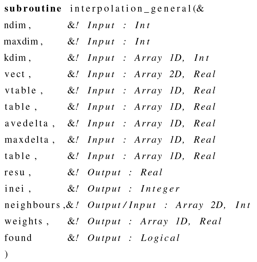
The list of input/output arguments is provided in Appendix C. In the main programme, calling the subroutine the key point is to transform first the N-dimension matrix into a 1-D array. An example of a main programme calling the subroutine is provided in the code package. The computation strategy in the subroutine can be broken down into the sequential steps as follows:

• i.

  Find the nearest neighbour of the input data by minimizing a distance with a simple incremental method stepping every ±1 coordinates on each dimension (detailed later in this section).

• ii.

  Scan the surroundings of the nearest point within the matrix on ±1 step on each dimension and store the corresponding block of input data to be tested. The size of the block is therefore $(\mathrm{1}+\mathrm{2}\times \mathrm{1}{)}^N$ but can be extended to $(\mathrm{1}+\mathrm{2}\times \mathrm{2}{)}^N$ if we increase the scanning process to ±2 on each dimension (hard-coded option iconf of 1 or 2 in the declaration block).

• iii.

  Calculate the distance to the previously selected input data. A p-distance concept is adopted (hard-coded option pnum in the declaration block). The pnum value p should be greater than or equal to 1 to verify the Minkowski inequality and be considered as a metric.

• iv.

  Sort the previous block of data in ascending order and stop the sorting process when the first 2^N point is selected. The code offers the possibility to use only the first N+1 neighbour (hard-coded option neighb in the declaration block) that is sufficient and faster in most cases.

• v.

  Calculate the weights and then the final result.

The first step consisting in finding the first neighbour is the trickiest and is broken down into several steps. Figure 2 displays an example in 2-D of the step-by-step procedure to find the nearest neighbour.

• i.

  The procedure initializes the process starting from the first point of the input data grid or taken from the last closest point if given in an argument as a non-null value.

• ii.

  A delta of coordinates is applied based on an average delta on each dimension to improve the initialization. This computation step of delta is externalized as it can be time consuming and should be done once for all target points at which we want to interpolate.

• iii.

  A test between the target value and the input data grid point coordinates determines the ±1 steps to add on each dimension (see Fig. 2 for an example in 2-D).

• iv.

  If the grid point falls on the edges or outside the borders, the closest coordinates within the matrix are selected.

• v.

  A test on the p-distance computation between the running point and the target is performed so that if the distance calculated at iteration N_it is equal to the distance at iteration N_it−2 the closest point is found.

• vi.

  If the distance is larger than the characteristic distance of the cell, the point is considered to be outside the borders of the input data grid. Therefore, the code allows a slight extrapolation if the target point is not too far from the borders.

• vii.

  At this stage, the procedure can stop if the distance to the closest vertex is 0, returning to the main programme with the exact value of the input data grid.

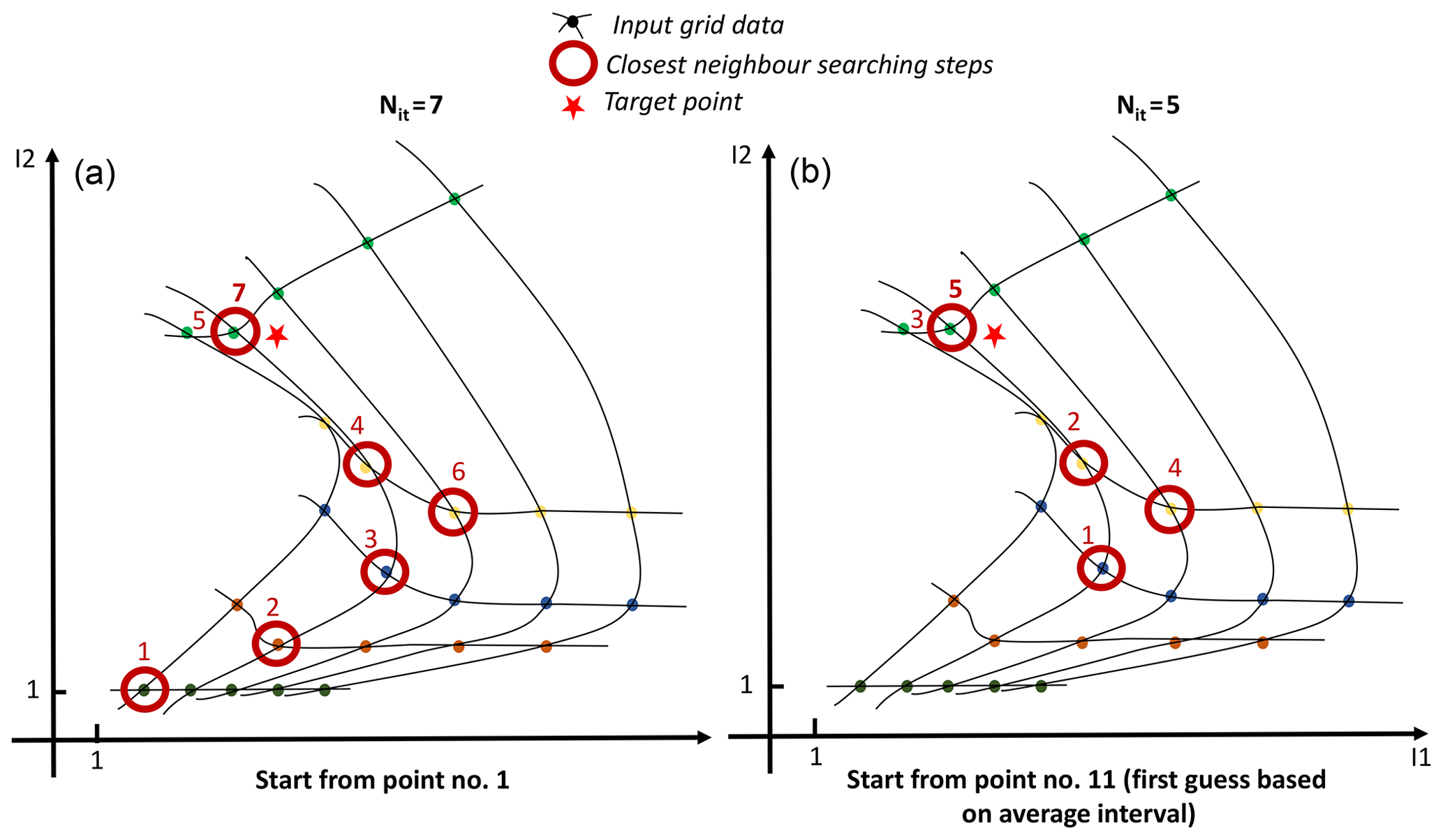
Figure 2 Real example in 2-D of the step-by-step procedure to find the nearest neighbour of a target point for an irregular but structured 5×5 grid (a) when starting the process from the first point of the grid on the lowest left corner and (b) when starting with a first guess based on an average delta computed for each dimension.

4 Visual example in 2-D for a regular grid

As an example to visualize the capacity of the general programme, the 2-D function used in Scipy (2014) is used to test our procedure. The function is

$$\begin{array}{}\text{(10)}& Y=f\left(X\right)=x_{\mathrm{1}}\times (\mathrm{1}-x_{\mathrm{1}})\times \cos \left(\mathrm{4}\mathit{\pi }{x}_{\mathrm{1}}\right)\times \sin (\mathrm{4}\mathit{\pi }{x}_{\mathrm{2}}^{\mathrm{2}}{)}^{\mathrm{2}},\end{array}$$

with $x_{\mathrm{1}},x_{\mathrm{2}}\in [\mathrm{0},\mathrm{1}]$.

Our input data grid is a regular grid with regular intervals of 0.02 from 0 to 1 for x₁ and x₂ with therefore 51 points on each dimension. We propose to interpolate on a finer regular grid with $n=\mathrm{100}\times \mathrm{100}$, 200×200 and 300×300 points on each dimension. For these three interpolation cases, a normalized mean square error (NMSE) of the result ${\stackrel{\mathrm{̃}}{Y}}_j$ for the full grid point number j can be calculated against the true value Y_j of the function as

$$\begin{array}{}\text{(11)}& \text{NMSE}={\displaystyle \frac{\frac{\mathrm{1}}{n}\sum _{j=\mathrm{1}}^n{\left({\stackrel{\mathrm{̃}}{Y}}_j-Y_j\right)}^{\mathrm{2}}}{\frac{\mathrm{1}}{n-\mathrm{1}}\sum _{j=\mathrm{1}}^n{\left(Y_j-\stackrel{\mathrm{‾}}{Y_j}\right)}^{\mathrm{2}}}},\end{array}$$

with $\stackrel{\mathrm{‾}}{Y_j}$ the mean value Y_j as $\frac{\mathrm{1}}{n}{\sum }_{j=\mathrm{1}}^n{Y}_j$.

For the three cases, the CPU time for the interpolation is evaluated and displayed in Table 1 for Machine 1 (Appendix E). As expected, the time consumption is obviously proportional to the number of points in which to interpolate. Figure 3 displays the evolution of the NMSE with the parameter p of the p-distance definition. There is a discontinuity of the NMSE from p=1 to $p={\mathrm{1}}^{+}$ with a slight increase with p in an asymptotic way (Fig. 4). The NMSE decreases with the number of points but a slight increase is observed from 200×200 to 300×300.

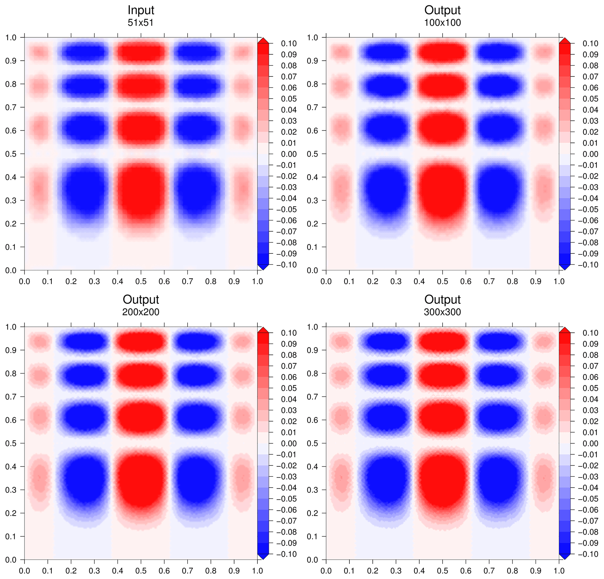
Figure 3 Interpolation results for the three cases. Figures were generated with the Generic Mapping Tools (Wessel et al., 2019).

Table 1 Performance for each case with p=1.

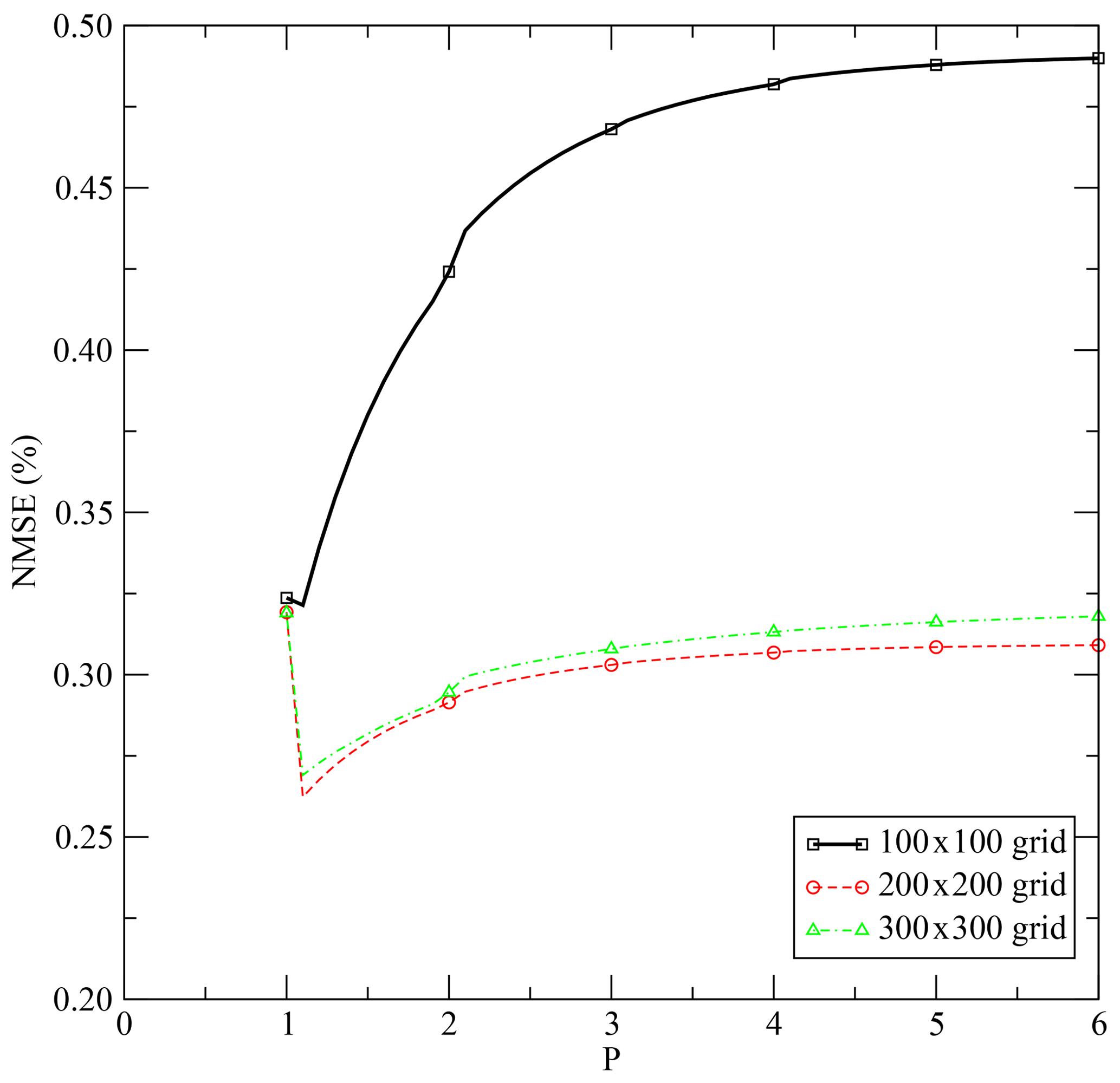
Figure 4 Evolution of performance based on the NMSE for the three cases as a function of the parameter p of the p-distance computation.

5 Example in 5-D for a regular grid

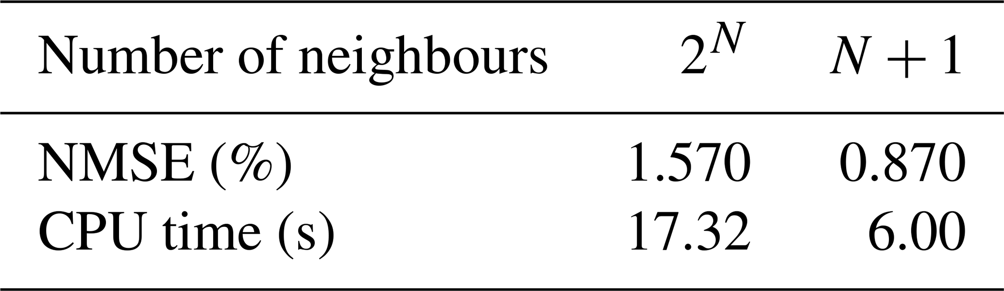
Still using the general programme, an example in 5-D (N=5) is proposed using the function

$$\begin{array}{}\text{(12)}& \begin{array}{rl}Y=f\left(X\right)=& x_{\mathrm{1}}\times (\mathrm{1}-x_{\mathrm{1}})\times \cos \left(\mathrm{4}\mathit{\pi }{x}_{\mathrm{1}}\right)\times \sin \left(\mathrm{4}\mathit{\pi }{x}_{\mathrm{2}}\right)\\ & \times \cos \left(\mathrm{4}\mathit{\pi }{x}_{\mathrm{3}}\right)\times \sin \left(\mathrm{4}\mathit{\pi }{x}_{\mathrm{4}}\right)\times \cos \left(\mathrm{4}\mathit{\pi }{x}_{\mathrm{5}}\right),\end{array}\end{array}$$

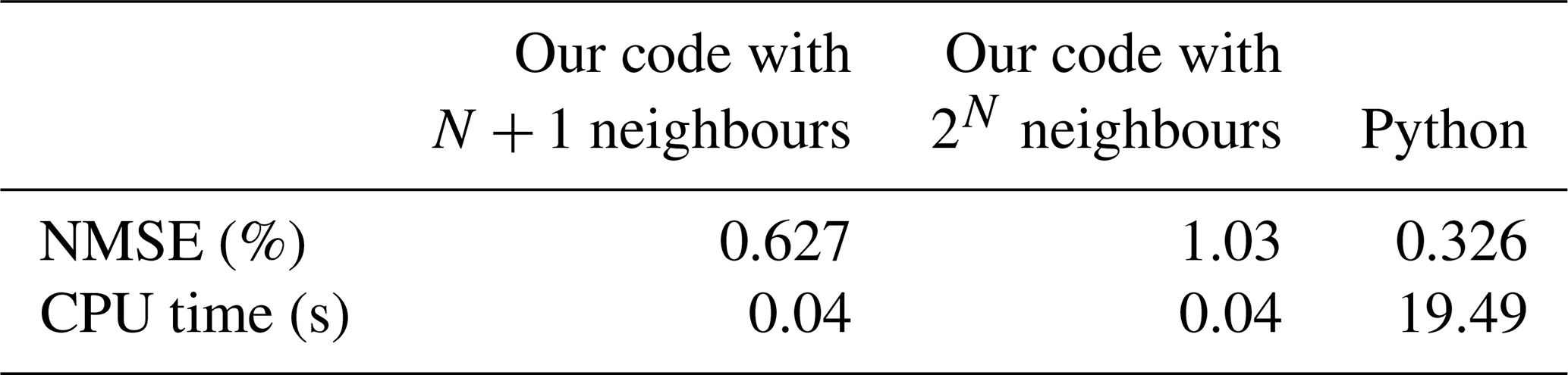
with $x_{\mathrm{1}},x_{\mathrm{2}},x_{\mathrm{3}},x_{\mathrm{4}},x_{\mathrm{5}}\in [\mathrm{0},\mathrm{1}]$. The input data grid is a regular grid of I_i=35 interval edges on each dimension $i\in [\mathrm{1},\mathrm{5}]$ with 35⁵=52 521 875 grid points. The goal is to find the results on a coarse grid of nine elements on each dimension with 9⁵=59 049 grid points. This case is an opportunity to test the influence of the number of neighbours in calculating the result. In our case, the parameter p of the p distance is set to p=2. The interpolation seems to provide better performance of the NMSE for our function with less neighbours (case N+1) and obviously with a lower CPU time (Table 2). This could certainly depend on the type of function to interpolate.

Table 2 Performance for the 5-D (N=5) case with p=2.

Another test with the 5-D case is performed to test the influence of the normalization as defined in Eq. (9) (flag norm) by defining an irregular grid still with 35⁵=52 521 875 input data points but with (i) random intervals values and (ii) one dimension depending on another. The definition of the input grid is defined in Appendix D and provided in the code package. With a similar order of magnitude of consumed CPU time, the normalization norm=.True. produces a NMSE of 0.499 % compared to the NMSE of 0.822 % for norm=.False. There is then an added value of using such a normalization with comparable CPU time consumption (rising from 2.68 to 3.44 s for our case).

6 Comparison with Python for a regular grid

The code has been tested against the Python procedure scipy.interpolate.griddata, freely available from Scipy (2014), for the following function:

$$\begin{array}{}\text{(13)}& \begin{array}{rl}Y=f\left(X\right)=& x_{\mathrm{1}}\times (\mathrm{1}-x_{\mathrm{1}})\times \cos \left(\mathrm{4}\mathit{\pi }{x}_{\mathrm{1}}\right)\\ & \times \sin \left(\mathrm{4}\mathit{\pi }{x}_{\mathrm{2}}\right)\times \cos \left(\mathrm{4}\mathit{\pi }{x}_{\mathrm{3}}\right),\end{array}\end{array}$$

with $x_{\mathrm{1}},x_{\mathrm{2}},x_{\mathrm{3}}\in [\mathrm{0},\mathrm{1}]$.

The input data grid is a regular grid of I_i=35 interval edges on each dimension $i\in [\mathrm{1},\mathrm{5}]$ with 35³=42 875 grid points. The goal is to find the results on a coarse grid of nine elements on each dimension with 9³=729 grid points. A case in 3-D has been used for this test because the Python library was not able to work with very large datasets (overflow error), while our programme could work perfectly. Here, scipy.interpolate.griddata is used with the bilinear interpolation option, while our method is configured with p=2.

Table 3 clearly shows how the Fortran code is faster compared to the Python library. However, the bilinear interpolation method seems to provide a higher accuracy than the inverse distance method embedded in our programme. Nevertheless, the error produced by our method looks acceptable.

Table 3 Comparison of performance between our code for a 3-D case with the grid data Python library. Machine 2 is used (Appendix F).

7 Geophysics application

7.1 The Backplumes model

In order to test this new interpolation programme, it is implemented in a back-trajectory model called Backplumes. This model was already used in some studies such as Mailler et al. (2016) and Flamant et al. (2018). Backplumes is open source and is available on the CHIMERE website. Backplumes calculates back trajectories from a starting point and a starting date. It is different from other back-trajectory models, such as the Hybrid Single-Particle Lagrangian Integrated Trajectory (HYSPLIT) (Stein et al., 2015), Stochastic Time-Inverted Lagrangian Transport (STILT) (Lin et al., 2003; Nehrkorn et al., 2010) and FLEXible PARTicle dispersion model (FLEXPART) (Pisso et al., 2019), because it launches hundreds of particles and plots all trajectories as outputs. Thus, the answer is complementary compared to the other models: the output result is all possible trajectories and not only the most likely.

An advantage of Backplumes for the WRF and CHIMERE users is that the code is dedicated to directly read output results of these models. Being developed by the CHIMERE developer teams, the code is completely homogeneous with CHIMERE in terms of numerical libraries. Another advantage is that the code is very fast and calculates hundreds of trajectories in a few minutes. Using the wind fields of WRF or CHIMERE, and running on the same grid, the results of back trajectories are fully consistent with the simulations done by the models.

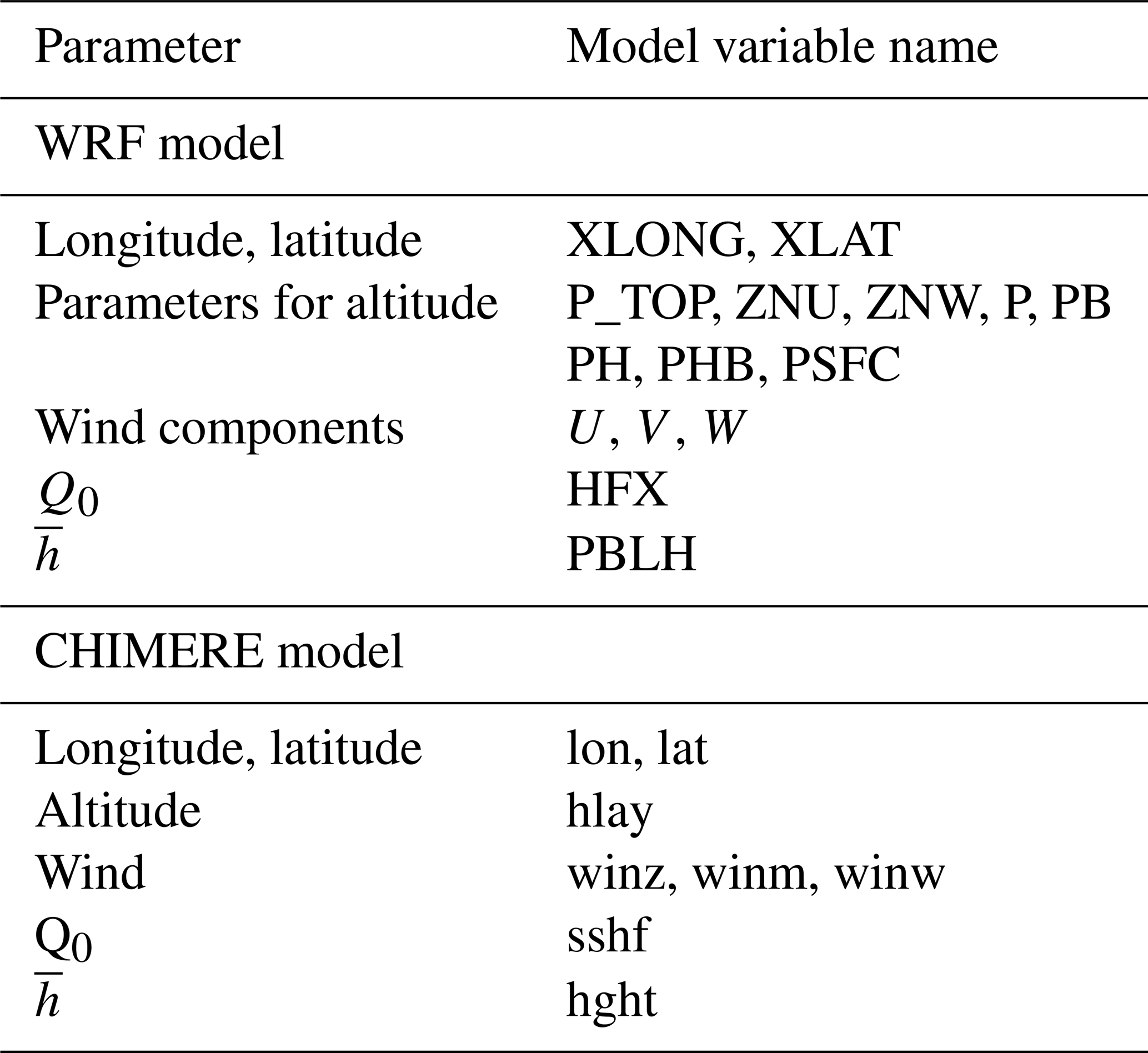
Backplumes is dedicated to calculate transport but not chemistry: only passive air particles (or tracers) are released. But a distinction could be made between gaseous or particulate tracers: for the latter, a settling velocity is calculated to have a more realistic trajectory. The model is easy to use and light because a small set of meteorological parameters is required. These meteorological parameters are described in Table G1 for WRF and CHIMERE.

The first step of the calculation is to choose a target location as a starting point. The user must select a date, longitude, latitude and altitude, obviously included in the modelled domain and during the modelled period. From this starting point, the model will calculate trajectories back in time. The number of trajectories is up to the user and may vary from one to several hundreds of tracers.

At each time step and for each trajectory, the position of the air mass is estimated by subtracting its pathway travelled as longitude Δλ, latitude Δϕ and altitude Δz to the current position. To do so, all necessary variables are interpolated with the NterGeo.v2020a interpolation programme described in the previous section. The calculation is described in Appendix G.

In order to respect the Courant–Friedrichs–Lewy (CFL) number, a sub-time step may be calculated. If the input data are provided hourly (as in many regional models), the meteorological variables are interpolated between the two consecutive hours to obtain refined input data.

The goal of Backplumes is to estimate all possible back trajectories. Then, starting from one unique point, it is necessary to add a pseudo-turbulence in the calculation of the altitude. Depending on the vertical position of the tracer, several hypotheses are made. Two parameters are checked for each tracer and each time step: (i) the boundary layer height enables us to know if the tracer is in the boundary layer or above in the free troposphere, (ii) the surface sensible heat fluxes enable to know if the atmosphere is stable or unstable.

When the tracer is diagnosed in the boundary layer, there are two cases: the boundary layer is stable or unstable. If the boundary layer is stable, Q₀<0, the tracer stays in the boundary layer at the same altitude. The new vertical position of the tracer is

$$\begin{array}{}\text{(14)}& z_{t-\mathrm{1}}=z_t.\end{array}$$

If the boundary layer is unstable, Q₀>0, the tracer is considered in the convective boundary layer and may be located at every level in this boundary layer for the time before this. Therefore, a random function is applied to reproduce a potential vertical mixing.

$$\begin{array}{}\text{(15)}& z_{t-\mathrm{1}}=\text{Rand}\times \stackrel{\mathrm{‾}}{h}\end{array}$$

The random function “Rand” calculates a coefficient between 0 and 1 to represent stochastic vertical transport of the tracer.

It is considered that 15 mn is representative of a well-mixed convective layer (Stull, 1988). If the time step is larger than 15 mn, the random function is applied. But if the time step is less than 15 mn, the vertical mixing is reduced to the vicinity of the current position of the tracer. In this case, we have

$$\begin{array}{}\text{(16)}& z_{t-\mathrm{1}}=\text{Rand}\times \mathrm{\Delta }z\times \left[z_t\right],\end{array}$$

where $\mathrm{\Delta }z=\frac{\mathrm{1}}{\mathrm{2}}\left(z_t^{k-\mathrm{1}}+z_t^{k+\mathrm{1}}\right)$ and k is the vertical model level corresponding to z_t.

In the free troposphere, the evolution of the tracer is considered to be influenced by the vertical wind component. A random function is applied to estimate its possible vertical motion with values between 0 and w∕2 m s⁻¹, representative of all possible values of vertical wind speed in the troposphere, Stull (1988). The vertical variability of the tracer's position in the free troposphere is calculated by diagnosing the vertical velocity as

$$\begin{array}{}\text{(17)}& z_{t-\mathrm{1}}=z_t-(\mathrm{0.5}+\text{Rand})w{\displaystyle \frac{\mathrm{3600}}{\mathrm{\Delta }t}}.\end{array}$$

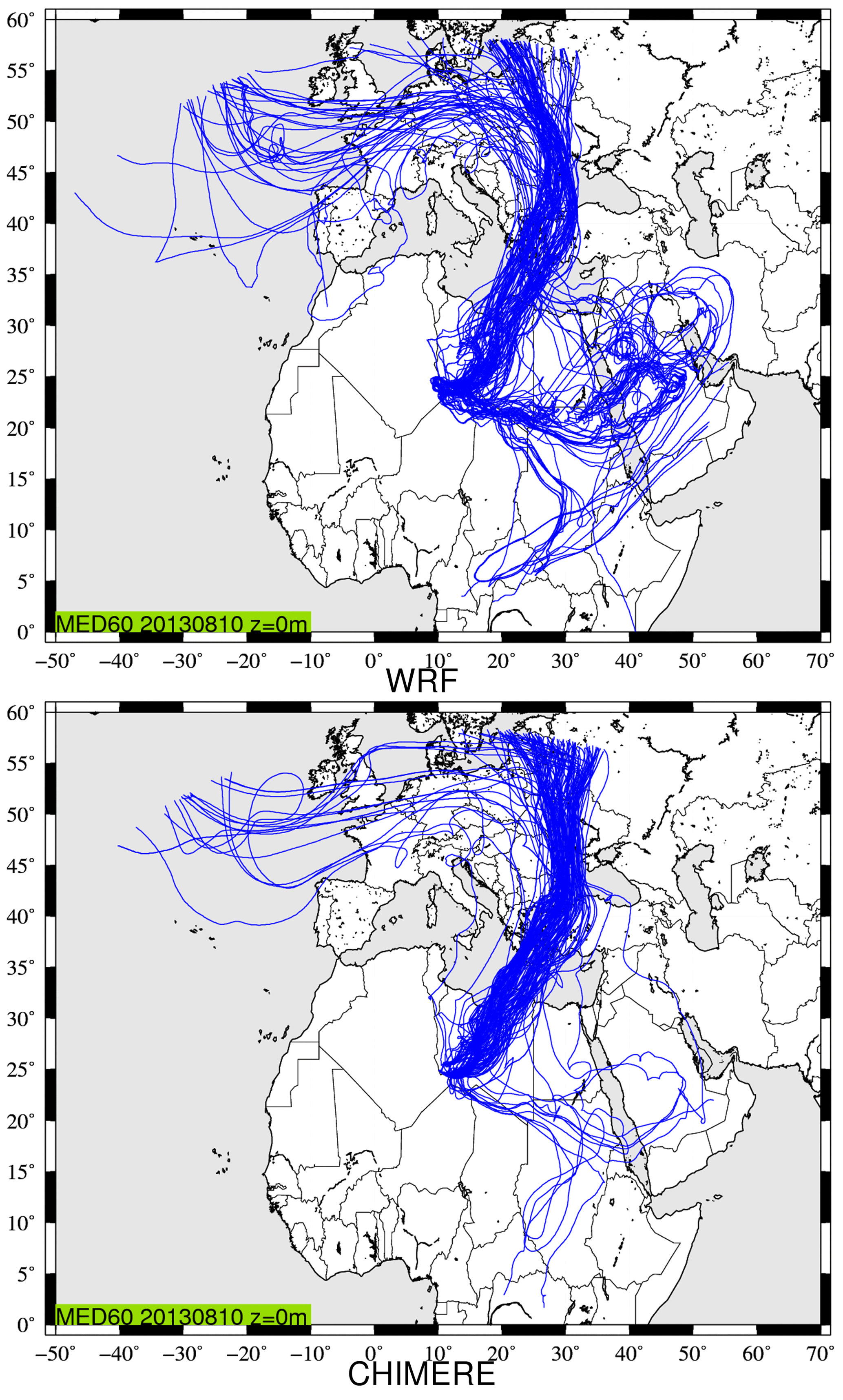
Figure 5 Back trajectories calculated using CHIMERE and WRF modelled meteorological fields. The starting point is at longitude 10^∘ E and latitude 25^∘ N, with an altitude of 0 m a.g.l. on 10 August 2013 at 12:00 UTC. It corresponds to a case studied during the Chemistry-Aerosol Mediterranean Experiment (ChArMEx) campaign (Menut et al., 2015).

7.2 Examples of back-trajectory computations

An example is presented for the same case and the WRF and CHIMERE models. The difference between the two models is the number of vertical levels (35 for WRF and 20 for CHIMERE, from the surface to 200 hPa). The online modelling system WRF-CHIMERE is used, meaning that the horizontal grid is the same (a large domain including Europe and Africa and with $\mathrm{\Delta }x=\mathrm{\Delta }y=\mathrm{60}$ km). The wind field is the same for both models: CHIMERE directly uses the wind field calculated by WRF. The boundary layer height is different between the two models, with WRF using the Hong et al. (2006) schemes and CHIMERE using the Troen and Mahrt (1986) scheme. The surface sensible heat flux is the same between the two models, with CHIMERE using the flux calculated by WRF. WRF has more vertical model levels than CHIMERE; thus, meteorological fields are interpolated from WRF to CHIMERE. It impacts the horizontal and vertical wind fields.

Figure 5 presents the results of back trajectories launched on 10 August 2013 at 12:00 UTC. The location is at longitude 10^∘ E and latitude 25^∘ N, with an altitude of 0 m a.g.l. This location is of no scientific interest but is in the middle of the domain, in order to have the longer trajectories. The complete duration of trajectories represents 10 d back in time. Overall, 120 trajectories are launched at the same position and time. They are randomly mixed when they are in the boundary layer to represent the mixing and the diffusion.

The most important part of the plume comes from the north of the starting point. For this main plume, the calculation is similar between the two models. Another large part of Backplumes is modelled at the east of the starting point. However, this fraction is mainly modelled with WRF but not with CHIMERE, where only a few trajectories are diagnosed. One possible explanation may be found by analysing the vertical transport of the trajectories.

Figure 6 Projection of all back trajectories on a single time–altitude axis.

Figure 6 presents all plumes displayed in the previous figure but projected along the same time–altitude axis. The differences between the two Backplumes results are mainly due to the calculation of the boundary layer height. When WRF diagnoses an altitude of ≈ 3000 m, CHIMERE diagnoses ≈ 2000 m, leading to different direction and wind speed. Then, this implies a split of the plumes with WRF but not with CHIMERE. This illustrates the sensitivity of the result to the driver model. But, in both cases, the answer in our case is clearly that the main contributions of the air masses located at the starting point are mainly coming from the north-east, crossing Tunisia and then the Mediterranean Sea and Europe. The main difference between the two calculations is the eastern part of the plume, which is more intense with WRF than CHIMERE.

8 Conclusions

A new interpolation programme written in Fortran has been developed to interpolate on N-dimensional matrices. It has been evaluated for several dimension cases up to N=5. The code is fast compared to similar Python routines and highly portable in existing geophysical codes. The interpolation programme works for any dimension N above 2 and is designed to work with irregular but structured grids (characterized by a size for each dimension) or look-up tables. Already used in its “regular” version in CHIMERE, the “general” programme has been tested on a new real application which calculates air mass back trajectories from two widely used atmospheric models: CHIMERE and WRF. This interpolation programme can be used for any application in geophysics and engineering sciences and also to explore large structured matrices.

Appendix A: List of frequently used abbreviations

AGL	Above ground level
CFL	Courant–Friedrichs–Lewy number
CHIMERE	National French CTM
CTM	Chemistry-transport model
CPU	Central processing unit
NMSE	Normalized mean square error
PBL	Planetary boundary layer
PSFC	Surface pressure
WRF	Weather Research and Forecasting model

Appendix B: Binary strategy

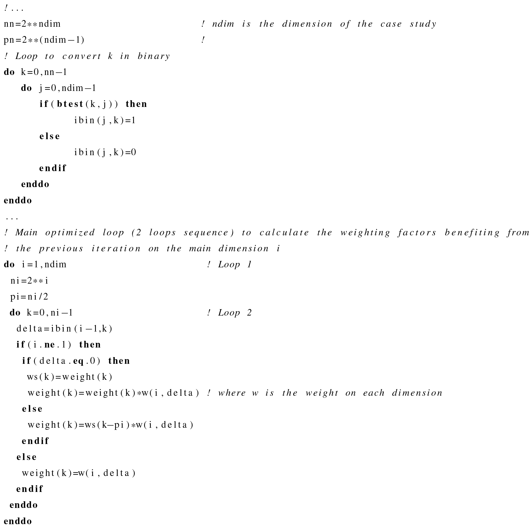
This piece of code shows the strategy to optimize the computation of weights for the “regular case”. The idea is to minimize the number of operations to benefit from the calculation at each dimension. A non-optimized loop would require 2^N−1 multiplications, while the optimized loop requires only ${\mathrm{2}}^{N+\mathrm{1}}-\mathrm{4}$ multiplications for the weight calculations. Then, for large values of N≫2, the ratio of required operations between the non-optimized and the optimized loop is $\approx (N-\mathrm{1})/\mathrm{2}$.

Appendix C: Code design

Note that avedelta and maxdelta arrays have been externalized to optimize the calculations. In the code package, an independent programme is available to calculate these arrays to be implemented in the user's main programme. The programme is written in Fortran double precision ingesting the following arguments:

Table C1 Description of subroutine arguments.

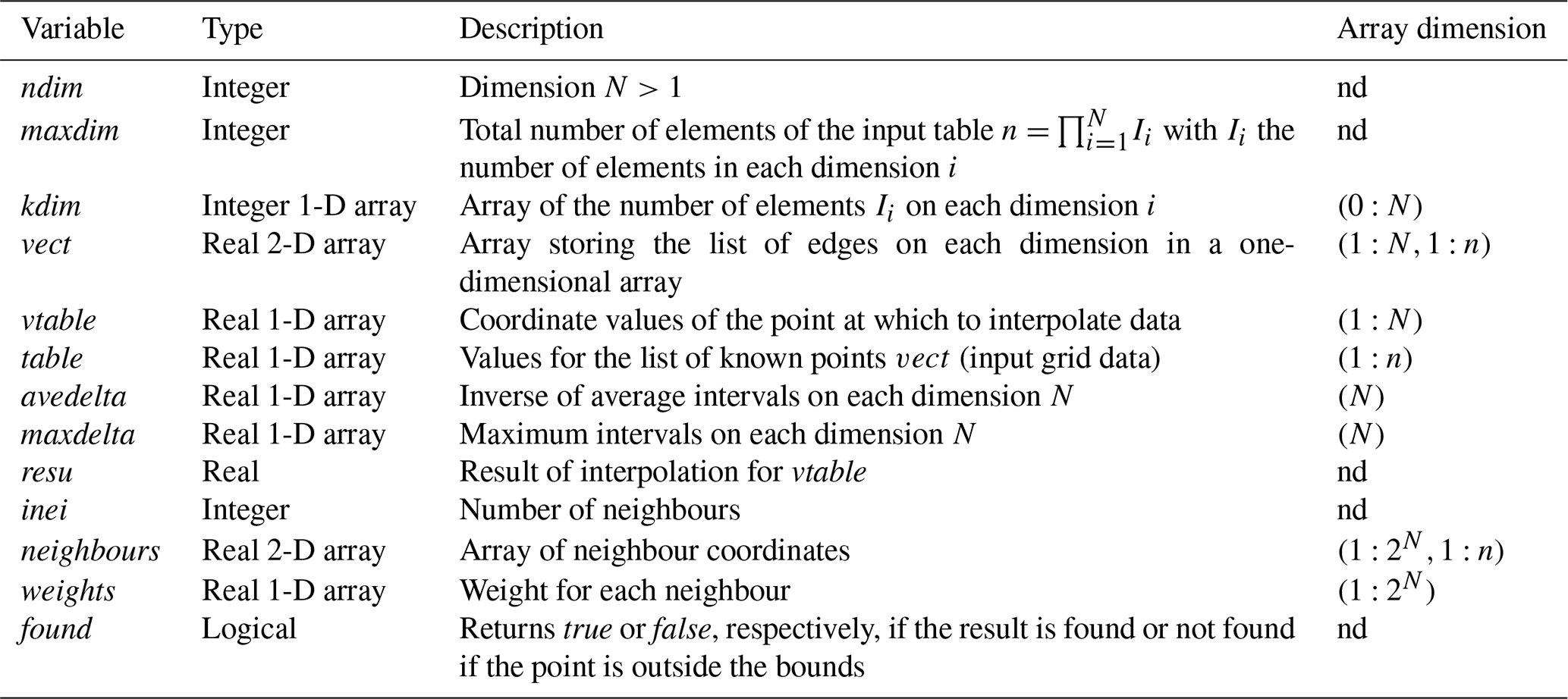
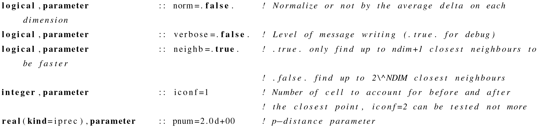
Some hard-coded variables can be tested by the user to improve the results. They have been tested and some results are described in this paper. A recompilation is necessary if the user changes these values.

Appendix D: Irregular structured grid example in 5-D

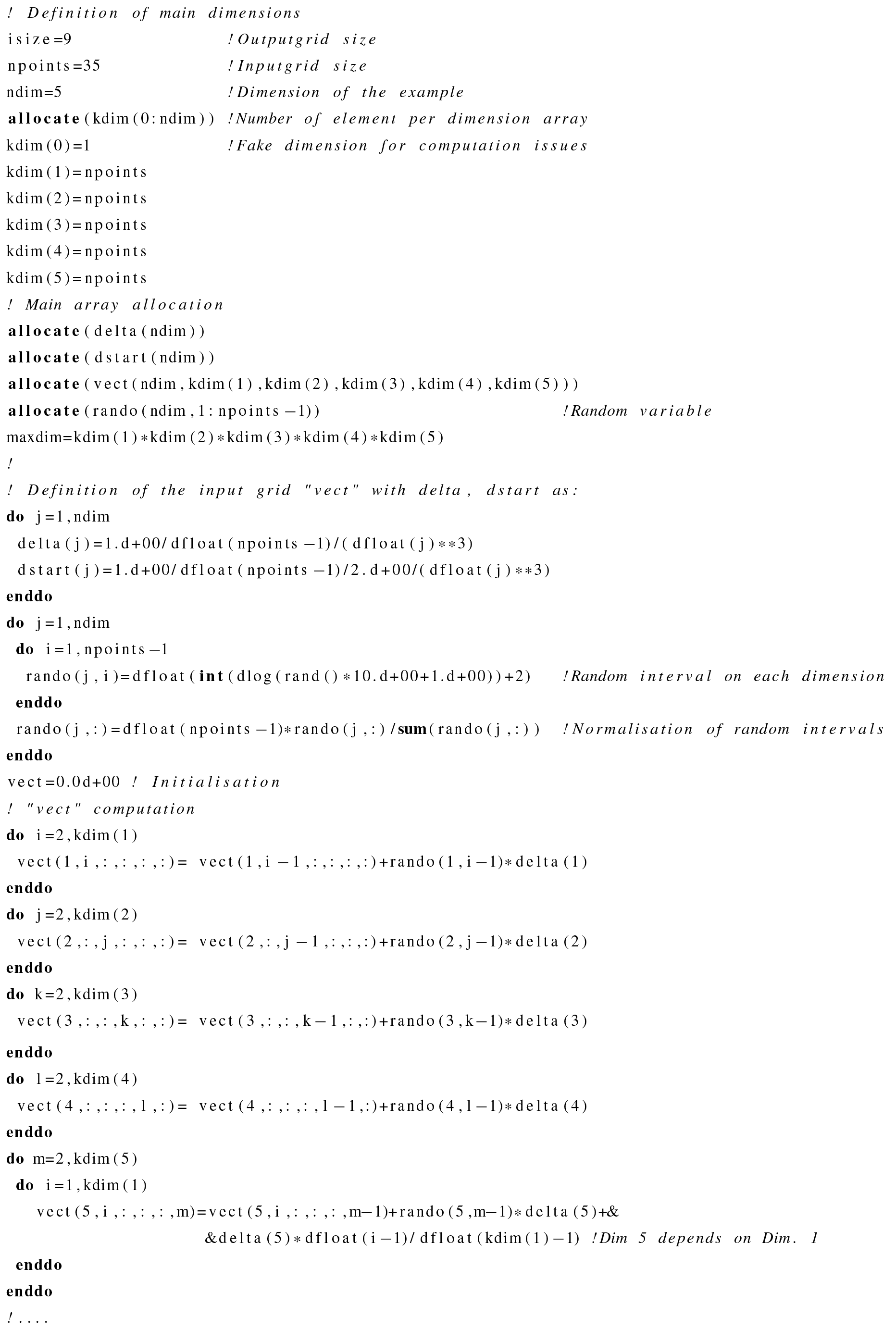
Below is an example of a 5-D array input grid data with irregular intervals with the last dimension (5) depending on dimension (1).

Appendix E: Characteristics of Machine 1

• Architecture: x86_64

• CPU op-mode(s): 32-bit, 64-bit

• Byte order: Little Endian

• CPU(s): 64

• Online CPU(s) list: 0–63

• Thread(s) per core: 2

• Core(s) per socket: 8

• Socket(s): 4

• NUMA node(s): 8

• Vendor ID: AuthenticAMD

• CPU family: 21

• Model: 1

• Model name: AMD Opteron Processor 6276

• Stepping: 2

• CPU MHz: 2300.000

• CPU max MHz: 2300.0000

• CPU min MHz: 1400.0000

• BogoMIPS: 4599.83

• Virtualization: AMD-V

• L1d cache: 16 KB

• L1i cache: 64 KB

• L2 cache: 2048 KB

• L3 cache: 6144 KB

• Memory block size: 128 MB

• Total online memory: 128 GB

• Total offline memory: 0 B

• Linux version 3.10.0-1062.12.1.el7.x86_64 (mockbuild@kbuilder.bsys.centos.org) (gcc version 4.8.5 20150623 (Red Hat 4.8.5-39)

Appendix F: Characteristics of Machine 2

• Architecture: x86_64

• CPU op-mode(s): 32-bit, 64-bit

• Byte order: Little Endian

• CPU(s): 96

• Online CPU(s) list: 0–47

• Offline CPU(s) list: 48–95

• Thread(s) per core: 1

• Core(s) per socket: 24

• Socket(s): 2

• NUMA node(s): 2

• Vendor ID: GenuineIntel

• CPU family: 6

• Model: 85

• Model name: Intel Xeon Platinum 8168 CPU at 2.70 GHz

• Stepping: 4

• CPU MHz: 2701.000

• CPU max MHz: 2701.0000

• CPU min MHz: 1200.0000

• BogoMIPS: 5400.00

• Virtualization: VT-x

• L1d cache: 32 KB

• L1i cache: 32 KB

• L2 cache: 1024 KB

• L3 cache: 33 792 KB

• NUMA node0 CPU(s): 0–23

• NUMA node1 CPU(s): 24–47

• Memory block size: 128 MB

• Total online memory: 190.8 GB

• Linux version 3.10.0-957.41.1.el7.x86_64 (mockbuild@x86-vm-26.build.eng.bos.redhat.com) (gcc version 4.8.5 20150623 (Red Hat 4.8.5-36)

Appendix G: The WRF and CHIMERE model parameters used

Parameters are the three-dimensional wind components, the boundary layer height $\stackrel{\mathrm{‾}}{h}$, the surface sensible heat flux Q₀ and the altitude of each model layer. The wind components are used for the horizontal and vertical transport. The boundary layer height is used to define the vertical extent of the possible mixing, and the surface sensible heat flux is used to know if the current modelled hour corresponds to a stable or unstable surface layer (for when the tracer is close to the surface).

Backplumes calculates the back trajectories using longitude, latitude and altitude in metres. In the case of input data with vertical levels in pressure coordinates, the altitude is calculated from pressure levels (Pielke, 1984). This is the case of the WRF model and the calculation is done as follows.

The altitude is computed as

$$\begin{array}{}\text{(G1)}& p^{*}=p_{\text{surf}}-p_{\text{top}},\end{array}$$

where p_surf (PSFC) is the surface pressure and p_top is the top pressure of the model domain. If p_top is constant over the whole domain, p_surf and thus p^* are dependent on the first level grid.

$$\begin{array}{}\text{(G2)}& z_{\mathrm{0}}={\displaystyle \frac{\mathrm{\Phi }\left(\mathrm{1}\right)+{\mathrm{\Phi }}^{\prime }\left(\mathrm{1}\right)}{g}},\end{array}$$

where Φ is the geopotential (PHB) and Φ^′ (PH) its perturbation at vertical level k. g is the acceleration of gravity, g=9.81 m s⁻². For each vertical level k, the layer thickness Δz and the cell top altitude z_k are estimated as

$$\begin{array}{}\text{(G3)}& \begin{array}{rl}& d_m=\log \left({\displaystyle \frac{p^{*}{\mathit{\eta }}_M-p_{\text{top}}}{p^{*}{\mathit{\eta }}_M+p_{\text{top}}}}\right)\\ & d_u=\log \left({\displaystyle \frac{p^{*}{\mathit{\eta }}_M-p_{\text{top}}}{p^{*}{\mathit{\eta }}_F+p_{\text{top}}}}\right)\\ & z_{\mathrm{1}}={\displaystyle \frac{\mathrm{\Phi }\left(k\right)+{\mathrm{\Phi }}^{\prime }\left(k\right)}{g}}\\ & z_{\mathrm{2}}={\displaystyle \frac{\mathrm{\Phi }(k+\mathrm{1})+{\mathrm{\Phi }}^{\prime }(k+\mathrm{1})}{g}}\\ & \mathrm{\Delta }z=(z_{\mathrm{2}}-z_{\mathrm{1}}){\displaystyle \frac{d_u}{d_m}}\\ & z\left(k\right)=z_{\mathrm{1}}+\mathrm{\Delta }z-z_{\mathrm{0}},\end{array}\end{array}$$

where η_M is its value on full (w) levels (ZNW) and η_F is the η value on half (mass) levels (ZNU). The layer thicknesses are space and time dependent; this calculation is performed for all trajectories and all time steps.

Table G1 List of parameters read by the Backplumes programme to calculate trajectories.

The new position of a tracer back in time is calculated as follows:

$$\begin{array}{}\text{(G4)}& \begin{array}{rl}& {\mathit{\varphi }}_{\text{rad}}=\mathit{\varphi }{\displaystyle \frac{\mathit{\pi }}{\mathrm{180}}}\\ & \mathrm{\Delta }x=u{\displaystyle \frac{\mathrm{3600}}{\mathrm{\Delta }t}}\\ & \mathrm{\Delta }y=v{\displaystyle \frac{\mathrm{3600}}{\mathrm{\Delta }t}}\\ & \mathrm{\Delta }\mathit{\lambda }={\displaystyle \frac{\mathrm{\Delta }x}{R\cos \left({\mathit{\varphi }}_{\text{rad}}\right)}}{\displaystyle \frac{\mathrm{180}}{\mathit{\pi }}}\\ & \mathrm{\Delta }\mathit{\varphi }={\displaystyle \frac{\mathrm{\Delta }y}{R}}{\displaystyle \frac{\mathrm{180}}{\mathit{\pi }}},\end{array}\end{array}$$

with the wind speed is provided in m s⁻¹ on an hourly basis, and R is the Earth's radius as R=6371 km. The new position for one tracer is thus

$$\begin{array}{}\text{(G5)}& \begin{array}{rlr}{\mathit{\lambda }}_{t-\mathrm{1}}& =& {\mathit{\lambda }}_t-\mathrm{\Delta }\mathit{\lambda }\\ {\mathit{\varphi }}_{t-\mathrm{1}}& =& {\mathit{\varphi }}_t-\mathrm{\Delta }\mathit{\varphi }.\end{array}\end{array}$$