the Creative Commons Attribution 4.0 License.
the Creative Commons Attribution 4.0 License.
 | 04 Feb 2021
The Meridionally Averaged Model of Eastern Boundary Upwelling Systems (MAMEBUSv1.0)
Jordyn E. Moscoso
Andrew L. Stewart
Daniele Bianchi
James C. McWilliams
Eastern boundary upwelling systems (EBUSs) are physically and biologically active regions of the ocean with substantial impacts on ocean biogeochemistry, ecology, and global fish catch. Previous studies have used models of varying complexity to study EBUS dynamics, ranging from minimal two-dimensional (2-D) models to comprehensive regional and global models. An advantage of 2-D models is that they are more computationally efficient and easier to interpret than comprehensive regional models, but their key drawback is the lack of explicit representations of important three-dimensional processes that control biology in upwelling systems. These processes include eddy quenching of nutrients and meridional transport of nutrients and heat. The authors present the Meridionally Averaged Model of Eastern Boundary Upwelling Systems (MAMEBUS) that aims at combining the benefits of 2-D and 3-D approaches to modeling EBUSs by parameterizing the key 3-D processes in a 2-D framework. MAMEBUS couples the primitive equations for the physical state of the ocean with a nutrient–phytoplankton–zooplankton–detritus model of the ecosystem, solved in terrain-following coordinates. This article defines the equations that describe the tracer, momentum, and biological evolution, along with physical parameterizations of eddy advection, isopycnal mixing, and boundary layer mixing. It describes the details of the numerical schemes and their implementation in the model code, and provides a reference solution validated against observations from the California Current. The goal of MAMEBUS is to facilitate future studies to efficiently explore the wide space of physical and biogeochemical parameters that control the zonal variations in EBUSs.
- Article
(1991 KB) - Full-text XML
- BibTeX
- EndNote


Eastern boundary upwelling systems (EBUSs) are among of the most biologically productive regions in the ocean, supporting diverse ecosystems and contributing to a significant portion of the global fish catch (Bakun and Parrish, 1982). The characteristic wind-driven upwelling dominant in EBUSs is forced by an equatorward meridional wind stress that decreases toward the shore, driving a zonal Ekman transport offshore. The resulting Ekman pumping brings cold, nutrient-rich water to the surface, fueling primary productivity (Jacox and Edwards, 2012; Chavez and Messié, 2009; Rykaczewski and Dunne, 2010).
The upwelling-favorable winds also drive baroclinic, equatorward geostrophic current, which sheds mesoscale eddies (Colas et al., 2013). Together with offshore Ekman transport, mesoscale eddies redistribute nutrients zonally and subduct nutrients and other tracers into the ocean subsurface (Capet et al., 2008; Gruber et al., 2011; Renault et al., 2016). The resulting cross-shore gradient of nutrients at the surface supports a zonal variation in the abundance of phytoplankton, with high biomass and chlorophyll nearshore, and low offshore (Chavez and Messié, 2009). The size structure of phytoplankton is similarly affected, with larger cells with higher nutrient demand onshore, and smaller cells offshore (Cabre et al., 2013).
While these qualitative patterns of productivity are common to upwelling systems, previous studies have shown that productivity varies substantially between EBUSs, but the causes of these inter-EBUS variations are not well understood. Possible physical drivers of these inter-EBUS variations include the shape and strength of the wind-stress curl, which set the upwelling strength and source depth (Bakun and Nelson, 1991; Jacox and Edwards, 2012). This in turn controls the energy transferred to the baroclinic eddy field, modulating surface nutrient availability via the “eddy quenching” mechanism (Gruber et al., 2011; Renault et al., 2016). Additionally, inter-EBUS variations may have biogeochemical origins, for example, due differing subsurface oxygen inventories (Chavez and Messié, 2009).
Our understanding of these drivers is hindered in part by the observational limitations and in part by the computational expense of regional models that can resolve the processes mentioned above. A range of models of varying complexity have been used to study EBUSs, from minimal two-dimensional (2-D) models (Jacox and Edwards, 2012; Jacox et al., 2014) to comprehensive regional models (Shchepetkin and McWilliams, 2005; Chenillat et al., 2018). While 2-D models require fewer computational resources than comprehensive regional model studies and thus allow a more comprehensive exploration of the relevant parameter space, they lack the explicit representation of important physical processes that affect biology in upwelling systems (i.e., eddy-quenching and meridional transport of nutrients).
Here, we aim to close the current gap in understanding by developing an idealized, quasi-2-D model of the physics and biogeochemistry of EBUSs. The model includes parameterizations of the key three-dimensional processes, while retaining the computational efficiency of a 2-D model. The model is cast in a residual-mean framework (Plumb and Ferrari, 2005a) in terrain-following coordinates (Song and Haidvogel, 1994) and is referred to as the Meridionally Averaged Model of Eastern Boundary Upwelling Systems (MAMEBUS). A schematic of all the important processes in MAMEBUS is shown in Fig. 1.
The rest of the paper is organized as follows. In Sect. 2, we describe the equations and physical parameterizations implemented in MAMEBUS, including general formulation of tracer advection and diffusion, the time-dependent turbulent thermal wind approximation of the momentum equations (T3W), eddy and boundary layer parameterizations, and our ecosystem formulation. In Sect. 3, we detail the algorithms and discretizations, including mesh specification, vertical coordinate transformation, and time integration. In Sect. 4, we describe the implementation of MAMEBUS including the various options available to the user, parameter choices, initialization, and output. In Sect. 5, we describe reference solutions for MAMEBUS, discussing model sensitivities to changes in bathymetry, wind forcing, and surface heat fluxes. Finally, in Sect. 6, we discuss further model development and future work.
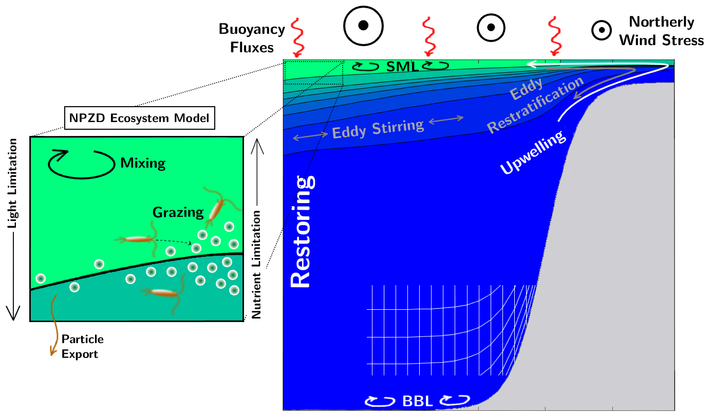
Figure 1A schematic of the essential components of the Meridionally Averaged Model of Eastern Boundary Upwelling Systems (MAMEBUS). This schematic highlights some components that the user is able to control including the offshore restoring conditions, the eddy mixing along isopycnals, the wind forcing, the surface mixed layer and bottom boundary layer parameterizations, and grid spacing.
MAMEBUS is comprised of a series of components that are necessary to capture physical–biogeochemical dynamics in EBUSs: (1) explicit momentum conservation in form of geostrophic, hydrostatic, and Ekman balances implemented as part of the T3W formulation; (2) eddies and their effect on material transport; (3) surface and bottom boundary layers; (4) nutrient and plankton cycles in form of a size-structured “NPZD”-type model (Banas, 2011).
With the exception of the velocity field, all tracers in MAMEBUS evolve according to the following conservation equation:
where the bar indicates a meridional average. The key physical tracer that follows Eq. (1) is temperature, θ, which serves as the thermodynamic variable in our model. We choose temperature as our thermodynamic variable because of its important effects on biogeochemistry (Sarmiento and Gruber, 2006). The biogeochemical tracers that are affected by the biogeochemical evolution term, , are a limiting nutrient N (here expressed in nitrogen units, akin to nitrate); a phytoplankton tracer, P; a zooplankton tracer, Z; and a detrital pool, D. The non-conservative terms, , represent physical sources and sinks of tracers, including surface fluxes, restoring at the offshore boundary, and optional restoring throughout the domain.
2.1 Tracer evolution
We first formulate an evolution equation for the meridionally averaged concentration of an arbitrary tracer c. We assume that c evolves according to a combination of advection by the three-dimensional ocean flow and diffusion by microscale mixing processes:
Here, u3 is the three-dimensional velocity vector, ∇3 is the three-dimensional gradient operator, and κdia the microscale diffusivity. In Eq. (2), we have assumed that the velocity field is non-divergent, i.e., . We further assume that u3 and c have already been averaged over a short timescale to exclude fluctuations associated with microscale eddies, whose effects are parameterized via the microscale mixing term (e.g., Aiki and Richards, 2008). We further simplify Eq. (2) by assuming that horizontal tracer gradients are small compared with vertical gradients, i.e., , as is typical for oceanic scales of evolution (e.g., Vallis, 2017). This implies that the microscale mixing acts primarily in the vertical, i.e.,
We now reduce the dimensionality of Eq. (3) by taking a meridional average, which we denote via an overbar:
Here, Ly is the meridional length of the region of interest and y is the meridional coordinate. Though we refer to this average as “meridional” throughout the text, for the purpose of comparison with EBUSs in nature, this average might be thought of instead as an along-coast average or as an average following isobaths, under the assumption that the additional metric terms introduced by such coordinate transformations are negligible. We next perform a Reynolds decomposition of the velocity and tracer fields:
where primes ′ denote perturbations from the meridional average. Taking a meridional average of Eq. (3) then yields
Here, we have used Eq. (5a)–(5b) and the property that perturbations vanish under the average, i.e., . We further define as the zonal–vertical gradient operator, and as the zonal–vertical velocity vector. The square bracket indicates the difference between vc at the northern and southern boundaries of the domain of integration, i.e.,
In its current form, Eq. (6) cannot be solved prognostically for because it includes correlations between perturbation quantities, i.e., the eddy tracer flux . Assuming that these perturbations are associated with mesoscale eddies, we parameterize the eddy tracer flux following Gent and McWilliams (1990) and Redi (1982). Specifically, we decompose the eddy tracer flux into advection of the mean tracer by “eddy-induced velocity” u⋆ and diffusion of along the mean buoyancy surfaces (see Burke et al., 2015):
Here, ∇∥ denotes the gradient along mean buoyancy surfaces (see Sect. 2.2. A more detailed derivation of Eq. (8) is given in Appendix A. We additionally simplify the meridional tracer advection term by assuming that , i.e., that the meridional tracer flux convergence is dominated by meridional tracer gradients, and that correlations between κdia and c are negligible, i.e., that the meridionally averaged vertical diffusive tracer flux serves to diffuse downgradient. With these simplifications, the full equation for the physical evolution of tracers is given by
The terms on the right-hand side of Eq. (9) are discussed further in the following sections: in Sect. 2.2, we discuss the evolution of the mean velocity via the momentum equations, and in Sect. 2.3 we discuss the subgrid-scale parameterizations, i.e., eddy advection, eddy stirring, and mixing.
2.2 Momentum evolution equations
To evolve a meridionally averaged tracer using Eq. (9), the meridionally averaged velocity field is required. This velocity field is evolved in MAMEBUS by solving a simplified form of the hydrostatic Boussinesq momentum and continuity equations with a linear equation of state (Vallis, 2017):
Here, is the dynamic pressure, where ρ0 is an arbitrary reference density, b is the buoyancy, θ is the potential temperature, α is the thermal expansion coefficient (assumed constant), g is the gravitational constant, and f is the Coriolis parameter. Note that we have assumed that momentum is mixed by microscale turbulence following the same diffusivity κdia as tracers (see Sect. 2.1), i.e., that the turbulent Prandtl number (e.g., Kays, 1994) is exactly equal to 1.
As in Sect. 2.1, we now meridionally average Eq. (10a)–(10e) to obtain evolution equations for and , and thus implicitly also for . This yields the following set of averaged equations:
Here, we have made the frictional–geostrophic approximation (e.g., Edwards et al., 1998), assuming that the Rossby number of the flow is small (e.g., Vallis, 2017), and thus that momentum advection (second terms from the left in Eq. 10a–10b) is negligible compared to other terms in the momentum equation. This assumption may indeed have some limitations in upwelling regions with steep topography and strong stratification. Lentz and Chapman (2004) show that in the cross-shelf momentum flux divergence balances the wind stress and supports an on shore return flow, which can impact nitrate concentrations on the shelf (Jacox and Edwards, 2011).
On the other hand, we have retained the time-evolution terms (leftmost terms in Eq. 10a–10b) to allow forward evolution of the horizontal velocity fields; if these terms were neglected, then these terms would need to be computed diagnostically at each time step. The resulting system is almost identical to the T3W equations (Dauhajre and McWilliams, 2018), a time-varying extension of the turbulent thermal wind balance (Gula et al., 2014), which was developed to explain the circulation of submesoscale fronts. The meridional pressure gradient in Eq. (11a) is imposed, rather than solved for prognostically, and is assumed to be set by the larger-scale subtropical gyre circulation encompassing the EBUS, which explicitly differs from the work done in Dauhajre and McWilliams (2018) which focuses on more rapid time-varying evolution on smaller scales. Together with the tracer advection equation for potential temperature (i.e., Eq. 9 with c=θ), Eq. (11a)–(11e) comprise a closed set of equations for the physical evolution of MAMEBUS.
In Eq. (11c), we have invoked the earlier assumption that (see Sect. 2.1), such that the averaged velocity field is non-divergent in the x–z plane. This implies that the zonal–vertical velocity field can be related to a mean stream function via
These relationships allow us to calculate and thus , from , subject to the boundary conditions
Here, is the mean sea floor elevation.
Additional boundary conditions are required to solve Eq. (11a)–(11e) prognostically. Specifically, we require that the vertical turbulent stress in Eq. (11a)–(11b) matches the wind stress applied at the sea surface and the drag stress at the sea floor, with the latter formulated via a linear drag law. Formally, these boundary conditions are
Here, r is a linear drag coefficient and is the meridional wind stress.
2.3 Physical parameterizations
In this section, we describe the parameterization of unresolved microscale mixing in the tracer evolution (Eq. 9) and the horizontal momentum (Eq. 11a–11b), and of mesoscale eddy advection and stirring in Eq. (9). This amounts to parameterizing the diapycnal diffusivity κdia, the isopycnal diffusivity κiso, and the eddy velocity u⋆.
2.3.1 Diapycnal mixing
We formulate the diapycnal mixing coefficient κdia as a sum of four distinct contributing processes: surface mixed layer turbulence (κsml), bottom boundary layer turbulence (κbbl), turbulence due to convective overturns within the water column (κconv), and background mixing due to internal wave breaking (κbg). Formally, we write
The terms on the right-hand side of Eq. (15) are discussed in turn in the following paragraphs.
The diapycnal diffusivity in the surface mixed layer, κsml, is prescribed to have the same structure as that used in the κ-profile parameterization (KPP) of Large et al. (1994). However, for simplicity, the mixed layer depth Hsml(x) and maximum magnitude κsml(x) are prescribed functions, rather than depending on the local surface forcing. The vertical profile of κdia in the surface mixed layer, i.e., , is given by
where the dimensionless surface mixed layer vertical coordinate is defined such that within the mixed layer. The structure function GKPP(σsml) is given by
following Large et al. (1994) and Troen and Mahrt (1986). The scaling factor of 27∕4 ensures that GKPP(σsml) has a maximum of 1 for .
The diapycnal diffusivity in the bottom boundary layer, κbbl, is prescribed in the same way as κsml but over the depth range . Thus, analogous to Eq. (16), we prescribe
where the dimensionless bottom boundary layer vertical coordinate is defined as .
At any point in space and time at which the water column is statically unstable, i.e., when N2<0, we increase the value of κdia is increased locally to parameterize the effect of density-driven convection. That is, we prescribe κconv following
Finally, the background diapycnal mixing, κbg(x,z), is simply prescribed as a constant background diffusivity. There are others that can be used (e.g., St. Laurent et al., 2002), but we opt for simplicity in the first version of this model.
2.3.2 Eddy advection and isopycnal mixing
We now discuss the formulation of the eddy advection and isopycnal mixing terms in Eq. (9). As discussed in Sect. 2.1, we follow the assumptions and formalism of the Gent and McWilliams (1990) and Redi (1982) parameterizations, which are commonly used in ocean models that do not explicitly resolve mesoscale eddies (e.g., Gent, 2011). These parameterizations assume that eddy-induced fluxes of buoyancy and tracer diffusion are directed along isopycnal slopes and so must be augmented in the ocean's surface mixed layer (SML) and bottom boundary layer (BBL). Here, the isopycnal slopes become very steep and isopycnals intersect the sea surface and floor (Tréguier et al., 1997). MAMEBUS therefore uses a modified form of the Ferrari et al. (2008) boundary layer parameterization, in which eddy buoyancy and tracer fluxes are rotated through the SML and BBL in order to enforce vanishing eddy-induced mass and tracer fluxes through the boundaries. Here, we summarize salient properties of this scheme, and in Appendix C we highlight differences between our scheme and that of Ferrari et al. (2008).
The eddy-induced velocity , introduced in Eq. (8), is non-divergent by construction (see Appendix A) and so we write it as
where ψ⋆ is the “eddy stream function”. This advecting stream function is assumed to be the same for all tracers, which is accurate in the limit of small-amplitude fluctuations of the velocity and tracer fields (Plumb, 1979), and takes the form
Here, κgm is the Gent–McWilliams diffusivity and the Sgm is the is the Gent–McWilliams slope. The latter is conventionally set equal to the mean isopycnal slope (Gent and McWilliams, 1990):
However, we allow Sgm to diverge from Sint in the SML and BBL, in part to ensure that the no-flux surface and bottom boundary conditions are satisfied (Ferrari et al., 2008):
Specifically, we prescribe
The formulations of the modified slopes Ssml and Sbbl are discussed below in the following sections (“surface mixed layer” and “bottom boundary layer” subsections).
The isopycnal mixing operator serves to mix tracers down their mean gradients, in a direction that is parallel to mean isopycnal surfaces in the ocean interior, following (Redi, 1982). This may be written componentwise as
where Siso denotes the slope of the surface along which the tracer is to be mixed and is assumed to be small (Siso≪1). Similar to Sgm, this slope is conventionally set equal to the mean isopycnal slope Sint, but we apply modifications to the formulation of Siso in the SML and BBL to ensure that there is zero eddy-induced tracer flux through the domain boundaries, i.e.,
where is a unit vector oriented perpendicular to the sea surface or sea floor. Specifically, we prescribe
Thus, Sgm and Siso are identical everywhere above the BBL. The need for a distinction within the BBL is explained below in the “surface mixed layer” and “bottom boundary layer” subsections.
Surface mixed layer
We now discuss the formulation of Ssml, the effective isopycnal slope in the surface mixed layer. Following Ferrari et al. (2008), we construct Ssml in a way that avoids singularities due to the vanishingly small vertical buoyancy gradients, and thus near-infinite isopycnal slopes, that occur in the mixed layer. This is achieved by using the vertical buoyancy gradient at the base of the mixed layer to define the effective slope as
where is a dimensionless vertical coordinate for the SML, as in Sect. 2.3.1. The corresponding eddy stream function (Eq. 21) is identical to that of Ferrari et al. (2008):
The structure function Gsml(z) is required to enforce continuity of the vertical tracer fluxes and flux divergences at the surface and at the base of the mixed layer. For example, Eq. (23) requires that Gsml vanishes at the surface:
We further require that the eddy stream function and eddy residual tracer fluxes be continuous at the base of the SML, i.e., that Ssml=Sint, which requires that
Finally, we require continuity of the divergence of the eddy tracer flux in order to avoid producing singularities at the SML base. The zonal and vertical components of the eddy tracer flux are
It may be shown that continuity of across is guaranteed if
where is a vertical length scale for eddy motions at the base of the mixed layer.
The simplest form for Gsml(z) that satisfies conditions for Eqs. (30), (31), and (33) is a quadratic function of depth:
Equation (34) is currently implemented in MAMEBUS. A more sophisticated form of Gsml that arguably has stronger physical motivation is given by Ferrari et al. (2008). They split the SML into a true mixed layer, in which Gsml varies linearly (and so the eddy velocity is approximately uniform), overlying a transition layer, in which Gsml(σsml) varies quadratically.
Bottom boundary layer
The scheme described above for the SML relies on the fact that the ocean surface is approximately flat, which allows the same effective slopes Ssml to be used for Sgm and Siso. The sloping sea floor requires separate BBL slopes, Sbbl and , and structure functions, Gbbl and , to satisfy the required conditions of no volume nor tracer flux through the boundary, i.e., Eqs. (23) and (26).
Analogous to the SML, we define the effective slope Sbbl as
where is the BBL vertical coordinate, as in Sect. 2.3.1. The eddy stream function in the BBL is therefore
To satisfy the condition of zero volume flux through the sea floor, Eq. (23), the effective slope must vanish at z=ηb(x), which requires
To ensure continuity of the eddy stream function at the top of the BBL, we require that Sbbl approach Sint, i.e.,
Finally, to ensure continuity of the eddy bolus velocity, we require that the gradient of Sgm be continuous at . This imposes a constraint analogous to Eq. (33) on Gbbl:
where is a vertical length scale for eddies at the top of the BBL. To satisfy Eqs. (37)–(39), we select a quadratic form for the structure function Gbbl(σbbl):
However, the effective slope Sbbl can no longer be used to define Siso in the BBL: Eq. (26) requires that the effective slope be aligned with the bottom slope at the sea floor, at . We must therefore employ a modified effective slope in the isopycnal mixing operator, as expressed in Eq. (27). We define as
where is a modified structure function that also vanishes at the ocean bed:
Continuity of the eddy tracer fluxes at the top of the BBL requires that
Finally, continuity of the eddy flux divergence is enforced by
To satisfy Eqs. (42)–(44), we select a quadratic form for the structure function :
2.4 Biogeochemical model formulation
The current biogeochemical model implemented in MAMEBUS is an NPZD (nutrient–phytoplankton–zooplankton–detritus) model. This NPZD model is modeled after the size-structured AstroCAT (Banas, 2011) and Darwin models (Ward et al., 2012). For the purpose of this paper, we reduced the size-structured ecosystem model to single phytoplankton and zooplankton size classes, while preserving the option to run multiple size classes in future versions of the model. We also include a detritus variable, which allows for sinking and export of organic matter away from the euphotic zone and redistribution of nutrients in the water column.
The biogeochemical equations in MAMEBUS are formulated similarly to previous NPZD models but cast in terms of the meridionally averaged nutrient, phytoplankton, zooplankton, and detritus concentrations. We neglect additional terms that would be introduced by first formulating the equations and then taking the meridional average, e.g., covariances of the type . This assumption is partially predicated on the idea that zonal gradients in biogeochemical tracers (e.g., nutrients and chlorophyll) are much stronger than meridional gradients, as supported by observations and models (Fiechter et al., 2018). For example, Venegas et al. (2008) show that average chlorophyll concentrations during the upwelling season vary approximately 2-fold in the northern California Current System, whereas observations from the California Cooperative Oceanic Fisheries Investigations (CalCOFI) (Fig. 7) show variations by an order of magnitude between nearshore and offshore stations. Along-shore gradients in chlorophyll are observed along the coast, where they are driven by wind and topographic variations; however, they are generally much smaller than the gradient between the coast and the offshore region (Fiechter et al., 2018). We recognize that this is a simplification of the true variability in EBUSs, but we consider it appropriate on average over the entire upwelling system, in particular within the idealized MAMEBUS framework, and plan to reassess it in future work.
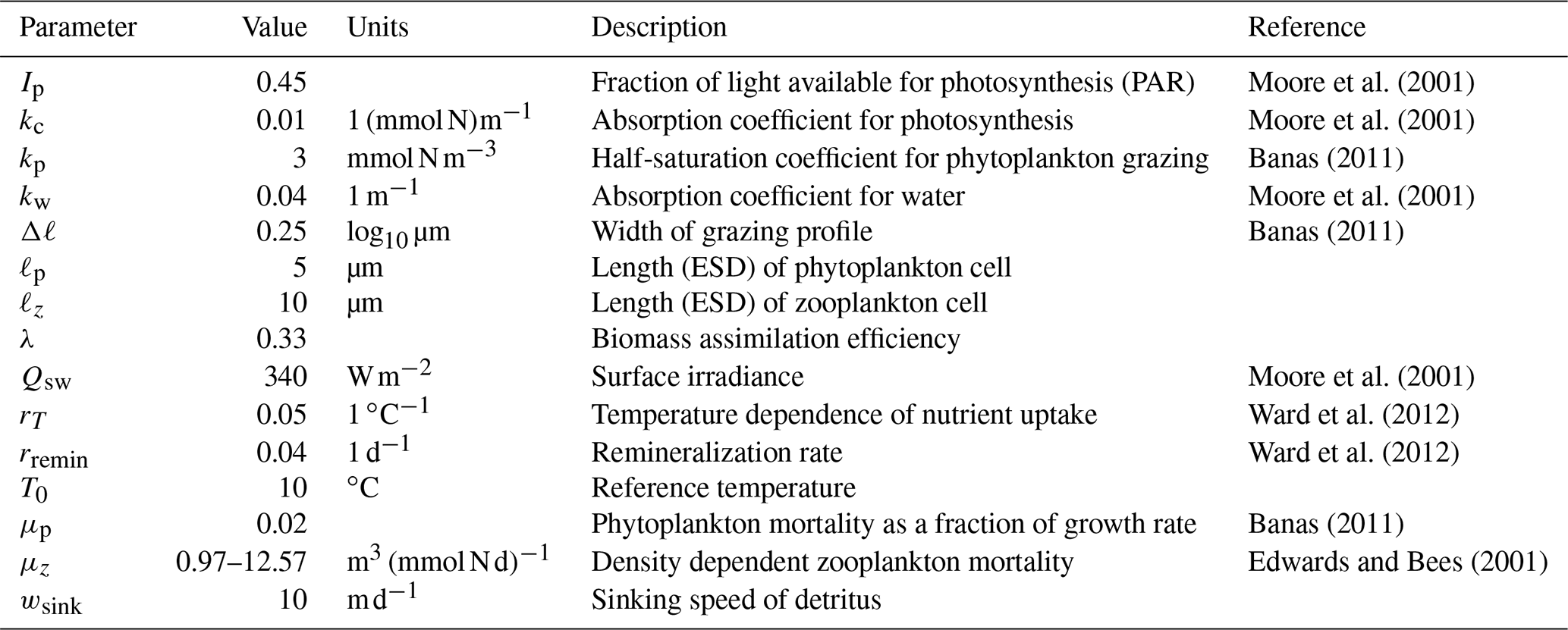
We drop the bar notation indicating a meridional average for this section, with the understanding that all variables denote meridionally averaged quantities. In the following, we include size-dependent uptake and grazing, along with variable sinking speeds for detritus, to retain essential size-dependent biogeochemical interactions and export fluxes. This will facilitate a future introduction of multiple size classes in the model. All variables and coefficients are given in Table 1. We note that all of the parameter values and equations described below measure time in days, whereas more generally MAMEBUS measures time in seconds; appropriate conversions are made in the model code to ensure dimensional consistency. The main conservation equations for biogeochemical tracers are
where T (∘C) is the model temperature, I (W m−2) is the local irradiance profile, N (mmol N m−3) is nitrate concentration, P (mmol N m−3) is phytoplankton concentration, Z (mmol N m−3) is zooplankton concentration, and D (mmol N m−3) is the detritus concentration. The terms on the right-hand sides of Eq. (46a)–(46d) are explained in the following subsections.
Moore et al. (2001)Moore et al. (2001)Banas (2011)Moore et al. (2001)Banas (2011)Moore et al. (2001)Ward et al. (2012)Ward et al. (2012)Banas (2011)Edwards and Bees (2001)Table 1Parameters and values used in the ecosystem model implemented in MAMEBUS. Coefficients without explicit references are chosen by the user.
2.4.1 Nutrient uptake
Common controls on phytoplankton population are bottom-up limitation (i.e., nutrient control), and top-down grazing by zooplankton (Sarmiento and Gruber, 2006). We formulate bottom-up controls using typical choices for light- and temperature-dependent terms, and Michaelis–Menten uptake (Sarmiento and Gruber, 2006). The functional form of uptake is given by
where φ(I) and φ(T) are light- and temperature-limiting functions, respectively. The light attenuation is modeled by integrating the Beer–Lambert law, following Moore et al. (2001):
and the light-dependent uptake function is modeled following Sarmiento and Gruber (2006),
The temperature component of the uptake function is
The maximum uptake rate is an allometric relationship defined as
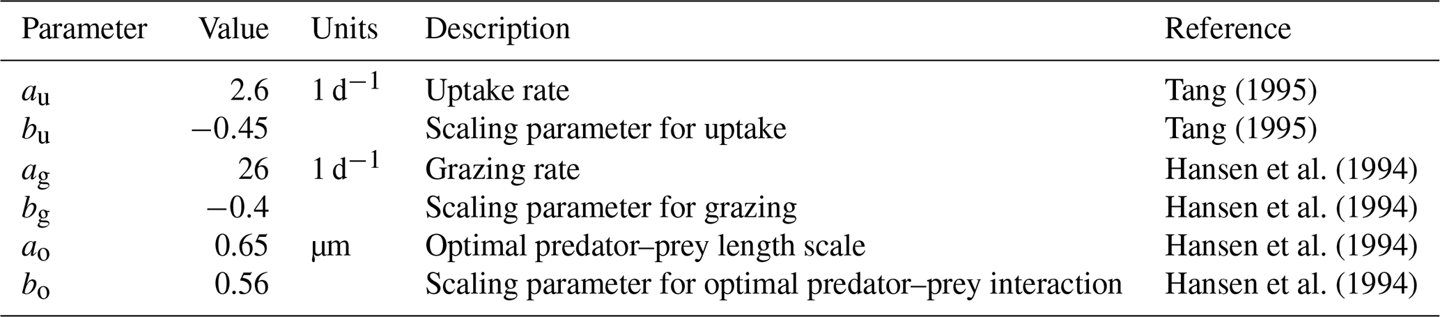
where ℓp is the user-determined phytoplankton size expressed as equivalent spherical diameter (ESD), and ℓ0=1 µm is a normalized length scale, with all allometrically defined variables listed in Table 2. While there are other options for the bases of these allometric relationships outlined in this section (e.g., cell volume), we make the decision to use ESD as a measure of cell size. Finally, the half-saturation coefficient is kN=0.1 mmol N m−3.
Tang (1995)Tang (1995)Hansen et al. (1994)Hansen et al. (1994)Hansen et al. (1994)Hansen et al. (1994)Table 2Parameters and values used in the ecosystem model implemented in MAMEBUS. Coefficients without explicit references are chosen by the user.
2.4.2 Grazing
Top-down processes are represented by zooplankton grazing on phytoplankton. Andersen et al. (2016) noted that there is an optimal length scale for active predation and grazing, as a strategic trade-off for optimal biomass assimilation. We make the assumption that the biomass assimilation of phytoplankton by zooplankton also follows Michaelis–Menten dynamics, then the functional form of grazing is given by
where the maximum grazing rate is defined by an allometric relationship defined as
where d−1 represents a “per day” quantity. We define a Gaussian distribution about an optimal grazing length-scale following Banas (2011):
where Δℓ sets the width of the optimal grazing profile and defines a band of grazing about the optimal prey size, ℓopt. By allowing for a variable band of grazing, we are able to control the assimilation efficiency of phytoplankton by zooplankton through direct preferential grazing. Accordingly, we model the optimal prey size based on a preferential grazing profile centered about an optimal predator–prey length scale:
2.4.3 Mortality
Mortality closure terms often set important internal dynamics in ecosystem models (Poulin and Franks, 2010). While linear mortality terms are generally used for phytoplankton, zooplankton mortality is often modeled via a quadratic term to avoid unrealistic oscillations and stabilize the solution (Poulin and Franks, 2010). The quadratic mortality term may be rationalized as a representation of mixotrophic grazing, zooplankton self-grazing, and higher-order grazing in NPZD models (Raick et al., 2006). Therefore, we model phytoplankton mortality as
and zooplankton mortality as
2.4.4 Remineralization and particle sinking
Sinking particles are an essential component of the vertical transport of nutrients from the surface to the deep ocean (Sarmiento and Gruber, 2006). Once particles sink past the euphotic zone, they are remineralized and returned to the subsurface nutrient pool. In this model, we represent remineralization processes via a linear rate, i.e.,
where rremin is the specific remineralization rate.
Particles sink at a constant average speed in the water column, following Eq. (46d). At the bottom boundary, we impose zero sinking flux, i.e., wsink=0 at . Thus, any nutrients that sink to the sea floor as detritus must remineralize there. This allows for redistribution of nutrients by mixing within the bottom boundary layer, diffusion into the interior, and transport via upwelling onto the shelf.
2.5 Non-conservative terms
In this section, we describe the treatment of all non-conservative terms in the tracer evolution equation. MAMEBUS allows arbitrary restoring of all tracers, which may be used, for example, to impose offshore boundary conditions or to impose restoring at the sea surface. Fixed fluxes of all tracers may also be imposed through the surface. More precisely, we formulate the non-conservative tracer tendency as
The restoring and surface flux components of this tendency are discussed separately below.
2.5.1 Restoring
The restoring of a tracer is represented as an exponential decay to a prescribed, spatially varying tracer field, , with timescale tr(x,z). The tracer restoring is then formulated as
2.5.2 Tracer fluxes
Surface fluxes are represented as a tendency in the tracer concentration in the surface grid boxes. For an arbitrary tracer c, we formulate the surface flux term as follows:
Here, is the downward flux of c (units of [c]m s−1) at the surface. For the case of buoyancy, the surface flux is imposed as a surface energy flux, Qs (W m−2), with
where Cp=4000 is the specific heat capacity.
In this section, we discuss the numerical solution of the model equations presented in Sect. 2. This entails a recasting of the equations in terrain-following, or “sigma”, coordinates (e.g., Song and Haidvogel, 1994; Shchepetkin and McWilliams, 2003), followed by the spatial discretization of the equations and algorithms for numerical time stepping.
3.1 Formulation in terrain-following coordinates
We solve the model equations presented in Sect. 2 in a coordinate system that “stretches” in the vertical to follow the shape of the sea floor. Such a coordinate system avoids “steps” in the sea floor that arise, for example, when using geopotential vertical coordinates and allows fine vertical resolution of the bottom boundary layer (e.g., Song and Haidvogel, 1994; Shchepetkin and McWilliams, 2003). Formally, we make a coordinate transformation , where σ is a dimensionless vertical coordinate and is defined such that σ=0 at z=0 and at . This transformation requires a relationship between z and σ via a transformation function
For example, a “pure” σ coordinate corresponds to the choice
where is the meridionally averaged water column thickness. However, this is not necessarily the most practical choice for numerical applications, in which it is useful to focus the vertical resolution over certain depth ranges (especially those close to the top and bottom boundaries of the ocean). MAMEBUS currently implements the UCLA-ROMS (Shchepetkin and McWilliams, 2005) transformation function:
Here, C(σ) is the stretching function, defined as
where
Here, C and are the bottom and surface components of the stretching function, respectively. The parameters and are surface and bottom stretching parameters; larger values cause the near-surface and near-bottom portions of the domain to occupy larger fraction of σ space. The parameter hc defines a surface layer thickness, in which the coordinate system is approximately aligned with geopotentials, provided that hb≫hc.
We now write the physical tracer evolution (Eq. 9) in σ coordinates. For a given function , we can write derivatives with respect to x and σ as
Using these identities, we may write the divergence of an arbitrary vector F, with components F(x) and F(z) in the and directions, respectively, as
Equation (69), combined with the definition of the mean stream function (Eq. 12), allows us to write the mean advection term in Eq. (9) as
An analogous expression may be obtained for the eddy advection term, , in Eq. (9), using the definition (Eq. 21) of the eddy stream function. Next, we apply Eq. (69) to the isopycnal mixing operator, defined by Eq. (25), in Eq. (9) to obtain
where Sσ=ζx is the slope of surfaces of constant σ in x–z space, i.e., the slope of the σ coordinate grid lines. Thus, the isopycnal mixing operator is essentially just modified by subtracting Sσ from Siso to obtain the mixing slope relative to the slope of the σ coordinate grid. Over most of the water column, Siso is equal to the isopycnal slope Sint, given by
Thus, the quantity Sint−Sσ can actually be computed more directly than the true isopycnal slope, as
Finally, the σ coordinate transformation of the vertical (quasi-diapycnal) mixing operator is
To summarize, we write Eq. (9) in σ coordinates as
where the tendency terms are
Here, we define
as the total advective or “residual” stream function (Plumb and Ferrari, 2005b), and we have added factors of ζσ in Eq. (76a) so that the fluxes can be directly identified with the zonal velocity, , and the dia-σ velocity, . Note also that every derivative with respect to σ is multiplied by , and that their product is equivalent to a derivative with respect to z. This allows us to simplify the numerical discretization by avoiding explicit references to σ coordinates and computing these derivatives via finite differencing in z coordinates.
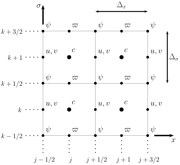
Figure 2Illustration of the numerical grid used to compute solutions to the model equations.
3.2 Spatial discretization of the tracer evolution equation
We solve Eq. (9) using the slope-limited finite-volume scheme of Kurganov and Tadmor (2000) for systems of conservation laws. We divide the domain into a grid of Nx by Nζ cells, with uniform side lengths Δx and Δζ in x/ζ space, as shown in Fig. 2. We store the cell-averaged value of at the center of the (j,k)th grid cell, which we denote as . The mean, eddy, and residual stream functions are most naturally defined at the cell corners, as this allows a straightforward calculation of the residual velocities at the cell edges:
Here, we use Δz as a shorthand for the spatially varying vertical grid spacing, defined as a centered difference between adjacent grid points. The vertical grid spacing is defined for all cell centers, corners, and faces:
where denotes the physical elevation of each grid point. Note again that ϖ is the velocity normal to the upper and lower faces of the grid cell and so differs slightly from the true vertical velocity w.
To compute the advective tendency, Gadv, the Kurganov and Tadmor (2000) scheme requires a linear interpolation of over each grid cell. The linear slopes in the x and ζ directions around are calculated via slope-limited finite differences between and its adjacent grid points:
with parameter . The “minmod” function evaluates to zero if its arguments have differing signs and otherwise evaluates to its argument with smallest modulus. The cell center estimates of the derivatives are then used to construct two different estimates of at each cell face via
Finally, advective fluxes are determined at the cell faces using an estimate of the maximum propagation speed in the system, which in our case is simply the residual velocity, and thus the fluxes reduce to an upwind approximation:
For this version of the model, the formulation of the Kurganov and Tadmor (2000) scheme considers only the maximum propagation speed of the momentum, u, and excludes the internal gravity wave speed which is supported with the momentum calculation in Sect. 2.2. As a result, this would alter the overall advective fluxes; however, we omit this in the current version of the model and note that the full formulation can be implemented here, but we choose to leave this calculation to be updated in a future version of the model. The advective tendency in (x,z) space is then computed via straightforward finite differencing of these fluxes:
The advective discretization (83) requires the residual stream function to be known on all grid cell corners, which allows the numerical fluxes to be computed at the cell edges. The mean stream function is computed from the mean velocity field via Eq. (12):
The eddy stream function (Eq. 21) depends on the “true” slope (Eq. 72) of the local contours, which we discretize as
The calculation of the derivatives with respect to x and z is described in Sect. 3.5. We then construct ψ⋆ on cell corners as
The tracer tendency due to isopycnal diffusion, Giso, is discretized following the formulation of Kurganov and Tadmor (2000) for parabolic operators.
where , , , and are computed via Eq. (81a)–(81d). In the interior, the isopycnal diffusion slope Siso=Sint and is calculated on cell corners via Eq. (85) and interpolated to cell faces via
The diffusive tendency is then computed via straightforward finite differencing of the H fluxes:
The tracer tendency due to diapycnal mixing, Gdia, is computed implicitly. During each time step, all other physical and biogeochemical tendencies are computed and used to advance forward one time step Δt, i.e.,
Here, n denotes the time step number, and denotes an estimate of at t+Δt (see Sect. 3.3 for details of the time-stepping schemes). The updated tracer concentration is then further modified via the addition of a “correction” due to diapycnal diffusion. At each longitude, or for each j, we solve
Equation (91) defines a tridiagonal matrix system of algebraic equations for the unknowns , which is inverted using the Thomas algorithm.
Finally, the meridional advection is discretized via a straightforward upwind advection scheme:
where v(c) denotes the meridional velocity on tracer points and cu denotes the upstream tracer concentration, defined as
Here, cN and cS are the tracer concentrations at the northern and southern ends of the domain, respectively. In all of the steps listed above, conditions of zero residual stream function and zero normal tracer flux are applied at the domain boundaries. These conditions are imposed by simply setting ψ† to zero on all boundary points and by setting the numerical fluxes (F, H, etc.) to zero on the boundary cell faces.
3.3 Temporal discretization
MAMEBUS evolves the model equations forward in time using Adams–Bashforth (AB) methods Durran (e.g., 1991) modified to allow for adaptive-time-step sizes. In this section, we outline the derivation of these methods and formally show the derivation in Appendix B. We implement the adaptive-time-step AB methods because this family of methods is numerically stable with our scheme for the momentum equations (see Sect. 2.2). We then describe the constraints on the time step imposed by the Courant–Friedrichs–Lewy (CFL) condition.
3.3.1 Adaptive-time-step Adams–Bashforth methods
Our time-integration scheme uses a family of time-step-variable Adams–Bashforth integrative methods. This specific formulation of the AB methods allows for the model time step to be adjusted dynamically following the CFL conditions described in Sect. 3.3.2. Consider a tracer quantity c that evolves according to
Here, the function f conceptually represents the entire model state, including the physical, biogeochemical, and non-conservative tendencies. We make a note here that the diffusive component of the time-integration step is calculated implicitly and not included in the ABIII integration step (see Eq. 91). We implement the third-order Adams–Bashforth, or ABIII method, in this version of the model as the default option for time integration.
The first two time steps require the lower-order methods. We implement a forward Euler for the first time step and a second-order AB scheme (defined below) for the second time step:
Here, the notation Δtn indicates the nth time step. Derivations for the adaptive-time-stepping ABII and ABIII methods are given in Appendix B.
3.3.2 CFL conditions
MAMEBUS selects each model time step adaptively to ensure that time stepping is numerically stable. The time step is chosen to ensure that the CFL conditions for each of MAMEBUS's various advective and diffusive operators, described in preceding subsections, are satisfied.
The time step for advection of tracers is limited by the timescale associated with advective propagation across the width of a grid box (Δx or Δz). These constraints can approximately be expressed as
(Durran, 2010). Here, uigw is the maximum horizontal propagation speed of internal gravity waves (Chelton et al., 1998):
Particulate sinking in the NPZD model is also calculated explicitly and constrains the time step via a similar CFL criterion:
where wsink is the sinking speed of the particles.
We apply additional constraints on the time step to ensure that diffusive operators are stable. The standard numerical stability criterion for a Laplacian diffusion operator is (Griffies, 2018)
where κ is a diffusion coefficient and Δs is the spatial grid spacing. In the horizontal (Δs=Δx, the diffusion coefficients that determine the diffusive time step are the eddy diffusion and isopycnal diffusion coefficients, when κ=κgm and κ=κiso, respectively. 1 In the vertical (Δs=Δz), the diffusive time step is determined by the diapycnal diffusivity, κ=κdia, and by the vertical component of the eddy and isopycnal diffusion operators, and , respectively (see, e.g., Ferrari et al., 2008).
3.4 Discrete momentum equations and barotropic pressure correction
In this section, we describe the discretization of the momentum equations presented in Sect. 2.2, specifically in Eq. (11a), (11b), and (11c). To facilitate our discretization, we split the pressure, ϕ, into barotropic and baroclinic components:
The barotropic and baroclinic components correspond to the pressure at the surface and the hydrostatic pressure variation with depth, respectively.
The numerical time integration is calculated in a series of steps which include an explicit calculation of the non-diffusive time step, an implicit calculation of the vertical diffusion, and a barotropic corrector step in order to ensure that the flow is non-divergent. The calculation of the explicit time step is outlined in Sect. 3.3 and Appendix B. In order to be numerically consistent with the calculation of the stream function, the mean horizontal velocities and are stored on the western face of each grid cell. In Fig. 2, these are labeled as the u points. The time step calculation is shown below, noting that the explicit components of the time step, ℰ{⋅} are calculated following the ABIII methods outlined in Sect. 3.3, and the implicit diffusion ℐ{⋅} is calculated following Eq. (91).
Given the mean momentum at time step n, , we first perform the explicit component of the time step to construct an estimate of , denoted as :
Note that the zonal barotropic pressure gradient, , is excluded from this equation; this will be revisited in the final component of the time step. The discretization of the horizontal pressure-gradient terms in Eq. (102) is described in Sect. 3.5.
We next compute the tendency due to vertical viscosity following Eq. (91), which we denote via the operator ℐ. We thereby construct a second estimate of the velocity at time step n+1, denoted as :
Finally, we apply a tendency due to the zonal barotropic pressure gradient, ensuring that mass is conserved in each vertical fluid column (Dauhajre and McWilliams, 2018):
as required by Eq. (11c). We formulate the barotropic pressure correction as
Substituting Eq. (105) into (104), we obtain
This implies that the tendency in the mean zonal velocity due to the zonal barotropic pressure gradient must serve to bring the depth-integrated zonal velocity to zero, i.e.,
The calculation of the vertical integral of is computed in the model using a Kahan sum (Kahan, 1965).
3.5 Horizontal pressure- and buoyancy-gradient calculations
Pressure-gradient calculations in σ coordinates have been long known to produce discretization errors from the misalignment of geopotential and σ coordinate surfaces and rely on large cancelations in the vertical gradient near steep slopes (Arakawa and Suarez, 1983; Haney, 1991; Mellor et al., 1994, 1998). We follow Shchepetkin and McWilliams (2003) to calculate the horizontal-pressure-gradient force and reduce the errors in horizontal gradient calculations, which otherwise produce large spurious along-slope currents in MAMEBUS (not shown). This algorithm has been extensively tested via its implementation in ROMS (Shchepetkin and McWilliams, 2003, 2005), so we omit our own tests of the pressure-gradient calculation scheme in this study. For numerical consistency, we also calculate horizontal buoyancy gradients, required to evaluate the isopycnal slope (see Sect. 3.2), using the same algorithm.
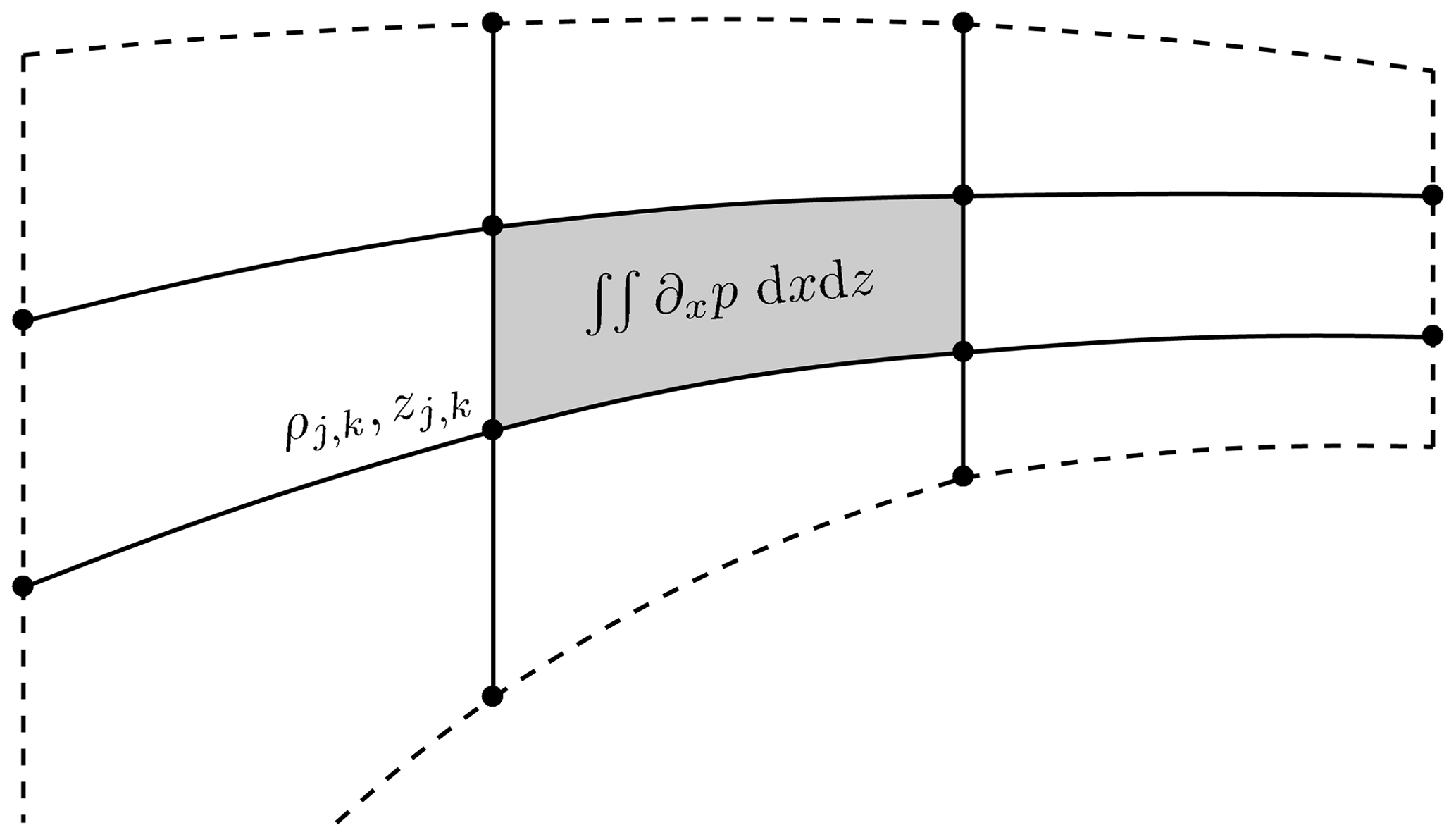
Figure 3Stencil for the isopycnal slope and pressure-gradient scheme given by Shchepetkin and McWilliams (2003). The points indicate the buoyancy (density) points. The solid lines are the reconstructed coordinate lines used in the horizontal calculation, and the shaded area shows the area integral of the horizontal buoyancy gradient.
3.5.1 Zonal pressure gradients
In this section, we outline the implementation of the zonal baroclinic pressure-gradient calculation used in MAMEBUS following Shchepetkin and McWilliams (2003). The ultimate goal of the algorithm is to calculate the following baroclinic pressure gradient at a cell center (see Eq. 102):
where ρ, like the linear case, is the density anomaly, ρ0 is a reference density, and A is the area between four adjacent buoyancy grid points (shaded area in Fig. 3). Shchepetkin and McWilliams (2003) calculate the second term by implementing a Lagrangian polynomial reconstruction of the z and ρ fields. By Green's theorem, we write the integrated horizontal density gradient as
The two algorithms differ on the treatment of the vertical integration of pressure. The density Jacobian algorithm first interpolates the density field onto the σ grid and calculates the values of ρ and z along the solid lines in Fig. 3, then integrates to obtain the pressure. The σ coordinate primitive form algorithm first integrates the pressure and calculates the gradients using a vertical correction term. We opt for the second algorithm which results in an equation for the horizontal gradient which closely resembles Eq. (68a). Furthermore, this algorithm tends to be more stable in our model. The algorithm is calculated as follows:
First, we calculate all elementary differences in ρ and z:
where zj,k is the depth value at the cell centers, where the density tracer is located. Note that the edges of Fig. 3 correspond to the cell centers in MAMEBUS; this requires some extrapolation at the boundaries so that the elementary differences are fully calculated throughout the domain. For all variables, we assume that the elementary differences at the boundary are zero.
We then calculate the hyperbolic differences of all variables. This step calculates an estimate of the derivatives following a cubic spline formalism outlined in more detail in Shchepetkin and McWilliams (2003). The derivatives are then given by
The vertical hyperbolic differences for ρ and z are calculated similarly using Eq. (110b) and (110d). Again, the hyperbolic differences on the boundaries are not defined using Eq. (111a) and (111b), so we extrapolate the hyperbolic averages of density. For example, at the western edge of the domain, we define
Analogous extrapolation schemes are applied at all domain boundaries.
We the calculate the pressure field using the hydrostatic relationship. This is done via a vertical integration of the density reconstructed along the vertical lines in Fig. 3. The pressure field is calculated from the surface down. The pressure is calculated in the surface grid cells as
where ζj=0 from the rigid lid assumption in MAMEBUS. Then the pressure is calculated at successively deeper grid levels as
We then correct for the iso-σ pressure gradient introduced by the slope of the σ coordinate grid, analogous to the continuous expression in Eq. (68a). This step calculates the product of ρ and the local slope of the σ coordinate and corrects for the interpolation errors from the coordinate transformation. Following the notation used in Shchepetkin and McWilliams (2003),
Finally, we use Eqs. (114) and (115) to calculate the pressure gradients:
Buoyancy gradients
The buoyancy gradient is calculated similarly to the pressure gradient. However, because we do not vertically integrate the buoyancy term, we opt to use the density Jacobian algorithm described in Shchepetkin and McWilliams (2003). The pressure-gradient algorithm described above integrates the pressure and then corrects for the pressure gradient in σ coordinates. The density gradient algorithm described below calculates the line integral about the area enclosed by the ϕ points where the buoyancy gradient is located (see Fig. 3). Therefore, we use the following form to calculate the buoyancy gradient:
where is the value of the integral (Eq. 117) along the vertical sides, and is the value of the integral along the horizontal sides. This calculation follows a similar procedure to the pressure gradient.
First, we calculate the elementary differences, and the hyperbolic averages in b and z, given by Eqs. (110a)–(111b). Then we calculate the value of the integral along the upper and lower sides of the domain following
Note that this formulation is the same as Eq. (115) but with buoyancy instead of pressure. Then we calculate the value of the line integral along the vertical components of the cell:
Shchepetkin and McWilliams (2003) write Eq. (68a) as
This allows us to numerically integrate the buoyancy gradient in the cell as
where A, again, is the area of the cell. At the surface, the boundary condition is given that
Finally, in order to calculate the horizontal buoyancy gradient, we divide by the area. Since the area of each cell is defined by the cell-centered ϕ points, we implement Gauss' area formula:
3.5.2 Meridional pressure gradients
The along-shore pressure gradient in Eq. (11b), denoted by , is determined by along-shore gradients in the surface pressure and buoyancy/density that are imposed as model input parameters. We integrate the profiles of pressure following the hydrostatic relationship. We define ρN and ρS as the densities at the northern and southern ends of the domain, and as the surface pressures at northern and southern ends of the domain. Then the pressure is given by
Here, the along-shore variations in sea surface pressure and density are both model inputs. We discretize the meridional pressure gradient as
Though MAMEBUS allows meridional pressure gradients to be imposed, we have excluded them from our reference solutions in the interest of simplicity. However, previous studies have highlighted the importance of meridional pressure gradients in supporting interior cross-slope transport and in driving poleward undercurrents Connolly et al. (2014). We plan to address the effects of meridional pressure gradients on EBUS ecosystem dynamics in future scientific studies using MAMEBUS.
In this section, we outline the details for implementation in MAMEBUS. The model code is written in the C programming language. The model expects various user inputs that include initial conditions, along with user-defined model calculation details in Table 4 that include, but are not limited to, the momentum calculation scheme and the time-stepping scheme. The MAMEBUS distribution includes sample MATLAB codes that package these user inputs.
The software needed to run this model includes
Our provided setup also includes example scripts for running the model on a cluster; however, this model can be easily run locally on a laptop or desktop on any operating system so long as the necessary software is installed. Table 6 shows run times for the model on both the cluster and a 2015 Mac laptop.
MAMEBUS has three active physical variables: the zonal and meridional momenta, and the temperature (buoyancy). The current implementation of the biogeochemical model has four active variables: nitrate (N), phytoplankton (P), zooplankton (Z), and detritus (D). A variable number of additional passive tracers may also be included.
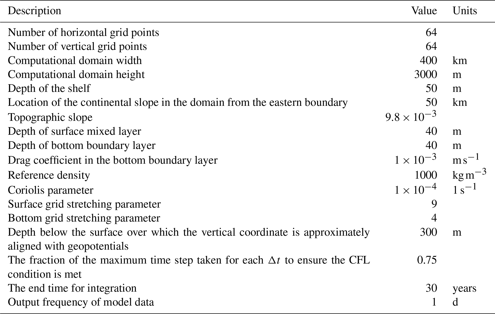
Table 3Input parameters expected by the MAMEBUS model code. All parameters listed in this table are chosen by the user. The sample values listed in this table are those used in the reference experiments described in Sect. 5.
4.1 Expected user inputs and options available
MAMEBUS expects a list of parameters given in Table 3 that control the physical components of the model, the model run details, and the grid setup. Other identifiers included in this model, given in Table 4, determine which internal schemes the model uses for each specific run. Furthermore, MAMEBUS expects a set of input parameters from physical tracers, forcing, diffusivity, and restoring, along with initial profiles of biogeochemical tracers that are listed in Table 5.
For the solutions shown in Sect. 5, the following initial conditions are detailed in Sect. 5.1.

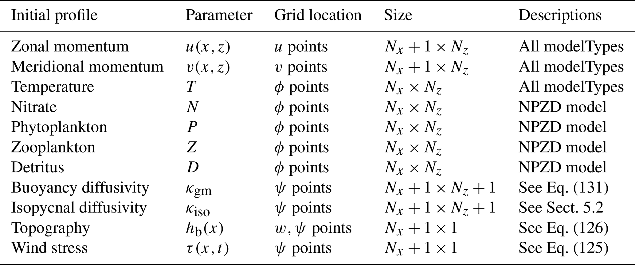
Table 5A table outlining the initial profiles that MAMEBUS expects during initialization. To visualize the grid locations, see Fig. 2. Each initial profile is included in “all modelTypes” unless otherwise stated. Note that Nx is the number of zonal domain points and Nz is the number of vertical domain points given in Table 3.
4.2 Model run details
The main function of the mamebus.c file has five major components and steps:
-
Calculate the time tendency of each tracer. The time step is calculated using the “tderiv” function detailed in Fig. 4. The explicit tendencies are calculated following Sect. 2.
-
Add implicit vertical diffusion and remineralization (Eq. 91).
-
Apply zonal barotropic pressure-gradient correction if the “momentumScheme” is MOMENTUM_TTW (Sect. 3.4).
-
Enforce zero tendency where relaxation time is zero (Sect. 2.5.1).
-
Write model state (Sect. 4.3).
4.3 Model data
All of the model input and output are saved in binary files. Depending on the “monitorFreq” or the frequency of output, the model will interpolate the between time steps, calculate the correct model state if necessary, and write the data to file. The following list contains all files that are written to file during the time-integration step. For each model, there is an option to include an arbitrary number of passive tracers; however, this is the standard list of tracers that are included in the indicated modelTypes.
-
Residual stream function, ψ† (all modelTypes)
-
Mean stream function, (all modelTypes)
-
Eddy stream function, ψ⋆ (all modelTypes)
-
Temperature field (all modelTypes)
-
Nitrate (NPZD model)
-
Phytoplankton (NPZD model)
-
Zooplankton (NPZD model)
-
Detritus (NPZD model)
In this section, we present reference solutions for MAMEBUS. Below, we discuss the choice of parameters, the non-conservative forcing, and profiles of restoring. We focus predominantly on the output of a single run and plan in the future to run parameter sweeps to better understand the response of the ecosystem dynamics to the physical forcing.
5.1 Model geometry, initial conditions, and forcing
The model is configured to represent an idealized California Current System (CCS). While the model can be formulated to represent a general EBUS, we use the California Current System as a test case because this allows comparison of our results with measurements from McClatchie (2016). Note that we exclude salinity as a physical tracer; while it may be important in determining the structure of the California undercurrent (Connolly et al., 2014), we find that the main features of stratification can be well described by temperature.
A list of input fields that MAMEBUS expects is given in Table 5, with a subset illustrated in Fig. 5. The solutions shown in Sect. 5 use the following choices for these input fields. The wind-stress profile is given by
where Lx is the width of the computational profile given in Table 3, and λτ=4 is a tuning parameter that controls the horizontal width of the wind-stress drop-off, or wind-stress curl. We tune the offshore maximum to approximate values reported by Castelao and Luo (2018). While this is the example of wind-stress forcing we choose to use to validate our model, any form of wind-stress forcing can be defined by the user.
The topography for the reference solutions is
where H is depth of the computational domain, Hs is the slope depth, xt is the location of the continental slope in the computational domain, and Lt is the width of the continental slope given from the topographic slope parameter. All parameters are given in Table 3. The topography is tuned to represent an idealized profile of bathymetry (ETOPO5; Eto, 1988) taken from the geographic coordinates given from line 80 in the CalCOFI data (McClatchie, 2016).
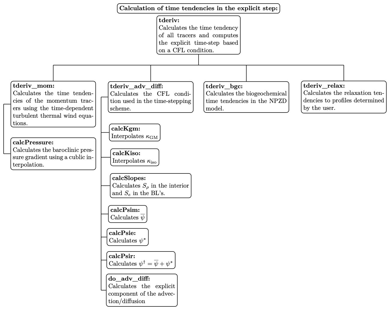
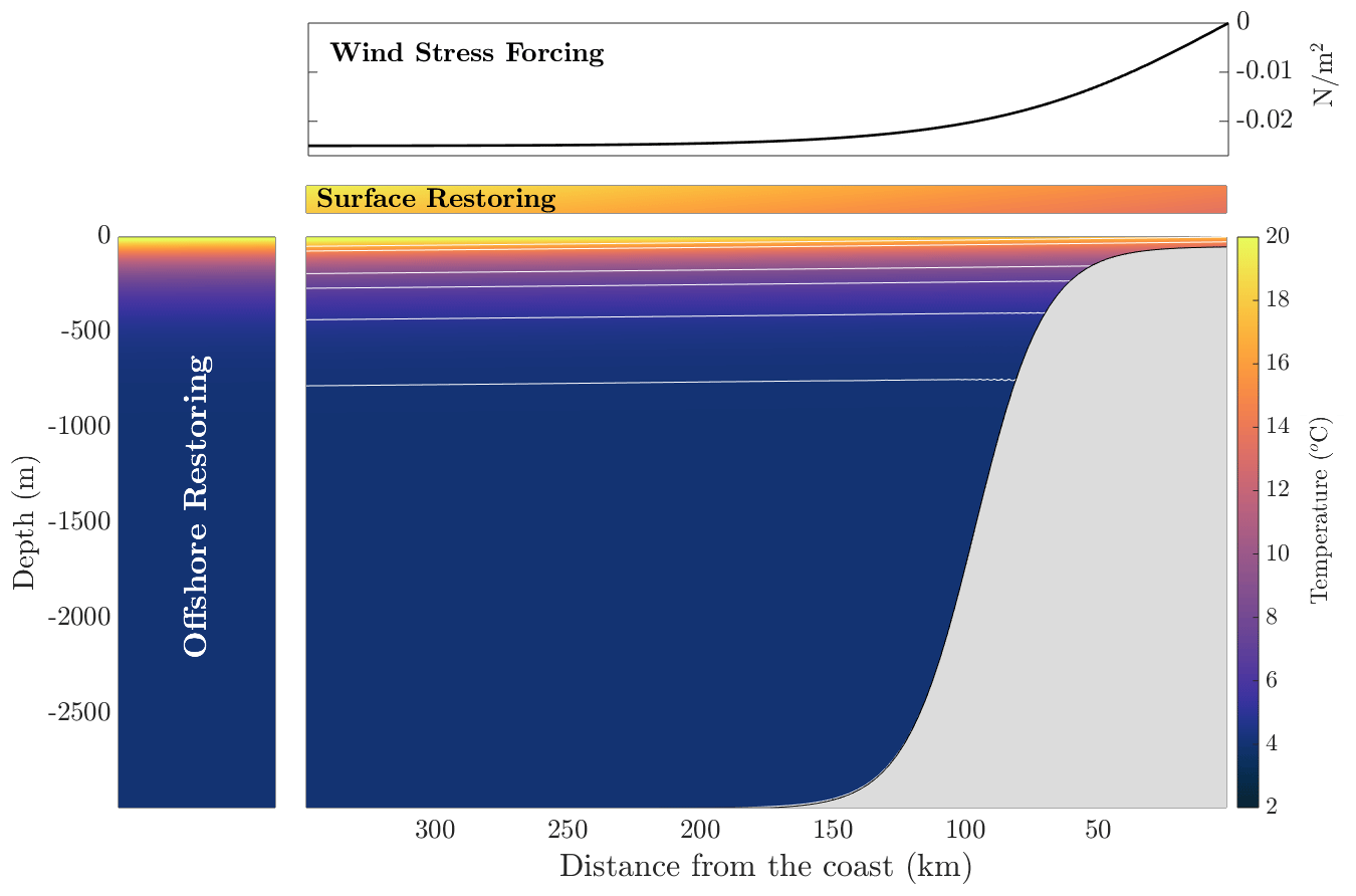
Figure 5Initial temperature profile with a profile of offshore restoring which is modeled as a sponge layer on the western side of the boundary, and at the surface, there is a surface restoring to an atmospheric profile, idealized to a profile of temperature from CalCOFI. The northward wind stress is shown at the top of the figure. The white lines in the temperature field are a few lines of constant initial temperature.
The initial conditions for the tracers in the model are the initial temperature profile, including timescales and inputs for restoring, and initial conditions for the NPZD model, which are tuned to give an approximate concentration of 30 mmol m−3 in the deep ocean. The biogeochemical tracers are not restored in this set of reference solutions. The initial profile of temperature is shown in Fig. 5 and given by
where the minimum and maximum temperatures in the domain are Tmin=4 ∘C, . The maximum and minimum surface temperatures are ∘C and ∘C, respectively. H⋆ is a decay scale for the temperature from the surface. This profile is tuned so that the temperature profile on the western side of the domain approximately matches the profile of temperature from CalCOFI (McClatchie, 2016) in Fig. 7. We initialize the temperature field with a small tilt in the isosurfaces to speed up the spin-up process. This same initial condition is used as the reference for temperature restoring. The timescale for restoring is given by
where Lr=50 km is the width of the sponge layer on the western side of the domain, and d is the fastest relaxation timescale for temperature. In the surface grid boxes, the restoring timescale is given by
which is consistent with the formulation of Haney (1971) for surface grid box thicknesses of approximately 1 m. The restoring at the surface grid box is set to the initial profile of temperature given in Eq. (127).
The initial conditions for NPZD tracers include a constant concentration of nitrate, Nmax=30 mmol m−3, phytoplankton, Pmax=0.02 mmol m−3, zooplankton, Zmax=0.01 mmol m−3, and an initial profile of detritus of zero. This choice allows for the internal ecosystem dynamics to control the biogeochemical solutions. Finally, the cell size we choose for the phytoplankton cell is ℓp=1 µm. The zooplankton cell is optimized to give the optimal predator–prey length scale between the phytoplankton and zooplankton interactions, i.e.,
5.2 Isopycnal, buoyancy, and diapycnal mixing
The unresolved mesoscale and microscale mixing in the tracer evolution Eq. (9) are detailed in Sect. 2.3.1 and 2.3.2, respectively. The diapycnal diffusivities are independent of wind stress and are determined by user-input mixed layer depth and maximum magnitudes. The isopycnal and buoyancy diffusivities are time-invariant fields whose spatial structure is prescribed by the user.
In our model reference configuration, the eddy and buoyancy diffusivities are functions of the baroclinic radius of deformation – the preferential length scale at which baroclinic instability occurs and closest to the fastest growing mode in the Eady model (Eady, 1949). In MAMEBUS, these diffusivities also exponentially decreases with depth. There are choices for more sophisticated parameterizations of eddy transfer across continental slopes (Wang and Stewart, 2018, 2020), but in this current version of the model, we opt for a simpler description. For example, the buoyancy diffusivity coefficient is defined as
where λ<1 is a tuning coefficient that allows for adjustment of the depth of the exponential profile of diffusivity, Hmax is the maximum depth of the topography offshore, and ηb is the depth of the topography. For all solutions shown in this section, λ=0.25. Note that for this formulation, we assume that z<0. The maximum buoyancy diffusivity is m2 s−1. Furthermore, κiso=2κgm, following Smith and Marshall (2009) and Abernathey and Marshall (2013). The isopycnal and buoyancy diffusivity profiles are shown in the left and center panels of Fig. 6, respectively.
The diapycnal diffusivities shown in the right panel of Fig. 6, with structure function described in Eq. (17), are set so that the maximum diffusivity in the mixed layers are given by m2 s−1; otherwise, the ambient diffusivity in the interior is given by m2 s−1. In the case where the mixed layers join at the eastern edge of the domain, the profiles of diffusivity are simply added.
5.3 Model validation
We run the reference solutions of MAMEBUS for 25 model years, with initial conditions and physical forcing described in Sect. 5.1. We validate the model against observations of temperature, nitrate, and chlorophyll a concentration in the euphotic zone, based on observations from the CalCOFI program (McClatchie, 2016). For this comparison, we interpolate a typical CalCOFI section (line 80) to a σ coordinate grid with realistic topography from the ETOPO database (Eto, 1988). We chose to validate our model with a single transect of from CalCOFI instead of several transects along the same line because averaging over time smooths over the deep chlorophyll maximum.
Furthermore, we prescribed a continental shelf that is deeper than in nature in order to reduce the model's computation time. Further shallowing the continental shelf is possible, but the CFL constraint imposed by the finer vertical resolution on the shelf extends the computation time.
While the continental slope is tuned to have a similar slope as observations in central California near the shelf break, the mixed layers in this model run are set to a constant depth zonally and overlap on the shelf. This choice has been made for simplicity and could be refined via zonally varying mixed layer depths to improve agreement with specific EBUSs. The well-mixed area on the shelf is an analogue to the inner shelf, albeit somewhat deeper than those found in nature (Lentz and Fewings, 2012). In our model comparison, we neglect the inner shelf region in the model and compare the solutions and starting approximately 50 km from the coast.
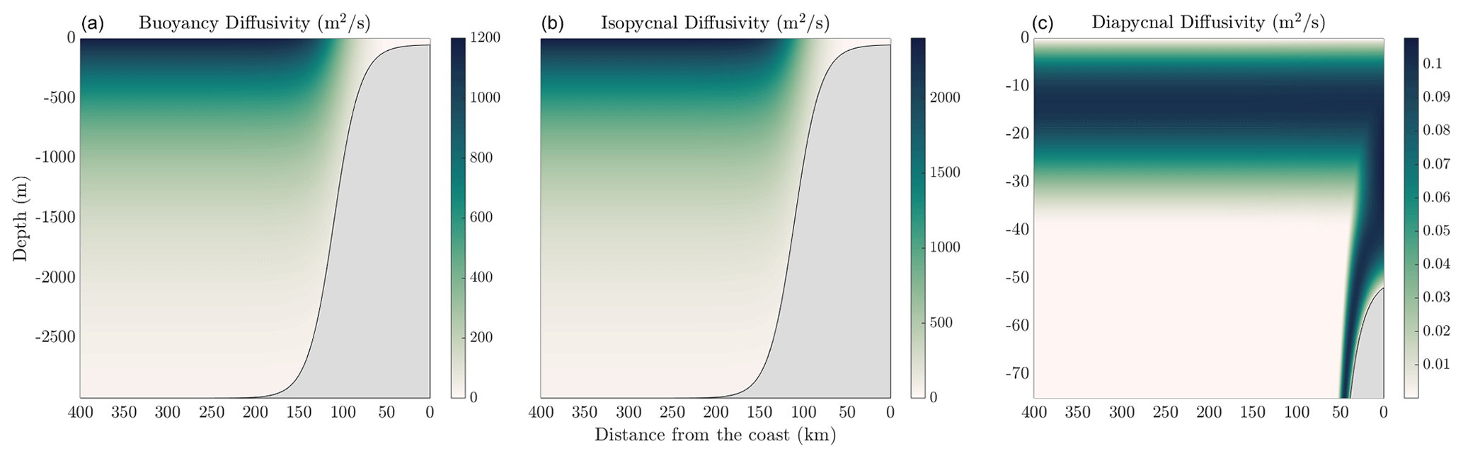
Figure 6Inputs of buoyancy diffusivity (a), isopycnal diffusivity (b), and diapycnal diffusivity (c) used in the reference solution to MAMEBUS shown in Sect. 5. Note that the isopycnal and diapycnal diffusivities are shown over the entire domain, and the diapycnal diffusivities are shown over the upper 75 m of the domain to highlight the boundary layer mixing and the mixing on the eastern side of the domain on the shelf where the boundary layers merge.
The model temperature is generally in good agreement with observations for the upper ocean, reproducing sloping isotherms towards the coast, and realistic surface values. We observe a cold bias near the coast, which could be a result of the constant wind-stress curl forcing over the domain, inducing upwelling that is too strong in the model. A cold bias observed in the surface just outside the shelf, and a warm bias offshore, are likely caused by the prescription of a constant mixed layer depth, which may be too deep in the model for this particular section and time of the year.
As shown by the middle row of Fig. 7, model nitrate agrees reasonably well with observations in the upper layers, although biases remain, in particular in deeper layers. This may be caused by several factors, including biases in the cross-shore and vertical circulation, and in the cycling of inorganic nutrients and organic matter. For example, remineralization processes are simplified in the model, which does not include dissolved organic matter, and represents export by a single particle size class with a constant sinking speed that was not explicitly tuned to match nutrients.
The bottom row of Fig. 7 shows that the model captures the main features of the observed chlorophyll distribution (here calculated based on a fixed chlorophyll to phytoplankton nitrogen ratio of 4:5 mg, chl m−3 : mmol N m−3 following Furuya, 1990). High surface concentrations are reproduced near the shelf, with values decreasing further offshore. A deep chlorophyll maximum develops in the lower euphotic zone, at depths between 40 and 80 m, progressively deepening from the coastal to the oligotrophic region offshore. While these patterns are fairly realistic, we note that the very high chlorophyll concentrations observed near the shelf are missing from the model. This underestimation may be caused by the oversimplification of the ecosystem structure in the NPZD model, which only includes a single phytoplankton group, while multiple groups are likely required for a more correct representation of enhanced coastal phytoplankton biomass (Van Oostende et al., 2018). Furthermore, aspects of these differences could be caused by the idealized nature of the 2-D circulation simulated by the physical model.
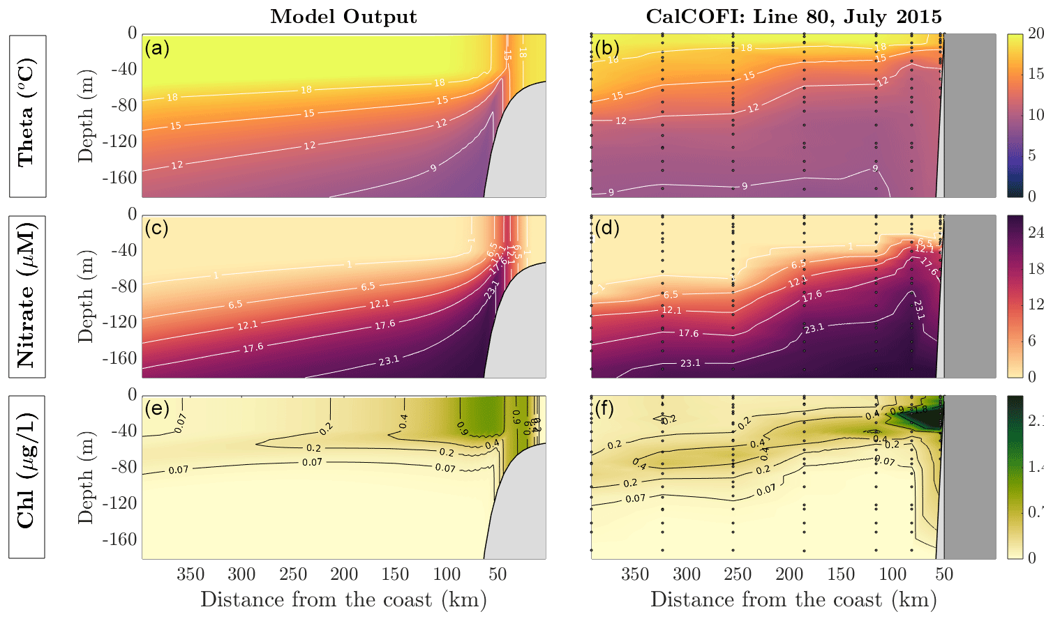
Figure 7Model validation against in situ CalCOFI data taken along line 80 (point conception) during July 2015. The column on the left shows output from the model under constant wind forcing and is averaged over the last 5 model years. The column on the right shows values taken from CalCOFI and interpolated onto a σ coordinate grid to allow for direct comparison. The dots in the panels are locations where the data are sampled. This figure shows the comparison between potential temperature, θ (a, b), nitrate (c, d), and chlorophyll concentration (e, f).
In order to compare physical solutions, we also include solutions which show the residual stream function, including the mean and eddy components in Fig. 8. The mean stream function is calculated via the momentum equations given in Sect. 2.2, whereas the eddy stream function is described in Sect. 2.3. The positive values indicate clockwise circulation, which, in this case, is indicative of eddy re-stratification opposing the mean upwelling branch (Colas et al., 2013). The negative values indicate counterclockwise circulation. Figure 8 shows that residual upwelling of waters onto the continental shelf via the bottom boundary layer, as interior transport onto the shelf is compensated by eddies. In the deep ocean (>500 m), there is a relatively strong residual overturning circulation that is likely associated with bottom intensification of the diapycnal mixing coefficient (e.g., McDougall and Ferrari, 2017).
5.4 Resolution parameter sweep
In this section, we describe the changes in solutions due to model resolution. We chose four different resolutions and explored the results. Figure 9 shows the solutions of MAMEBUS after 30 model years. Each panel in Fig. 9 shows the model state in the euphotic zone, averaged over the final 10 years of integration. All resolutions have the same setup and forcing as described in Sects. 4 and 5. The top row shows the potential temperature (θ), the middle row shows the nitrate concentration, and the bottom row shows the phytoplankton concentration. The model grid resolution increases from left to right, with the coarsest simulation run on a grid of 32 points horizontally and vertically, and the highest-resolution simulation run on a grid of 128 points horizontally and vertically.
Increasing the resolution leads to an overall shoaling of nutrients toward the surface. The largest overall change in near-slope nutrient concentration occurs when the resolution doubles from 32 to 64 horizontal points and vertical levels. Increasing the resolution beyond a 64×64 grid does not substantially change the horizontal distribution of phytoplankton. As referenced in Table 6, doubling the resolution increases the model run time by a multiple of approximately 20. Thus, while the model can practically be run at higher resolution, our tests show that intermediate resolution (64 horizontal and vertical levels) is sufficient to produce a favorable comparison with in situ data, without substantially increasing the computation time.
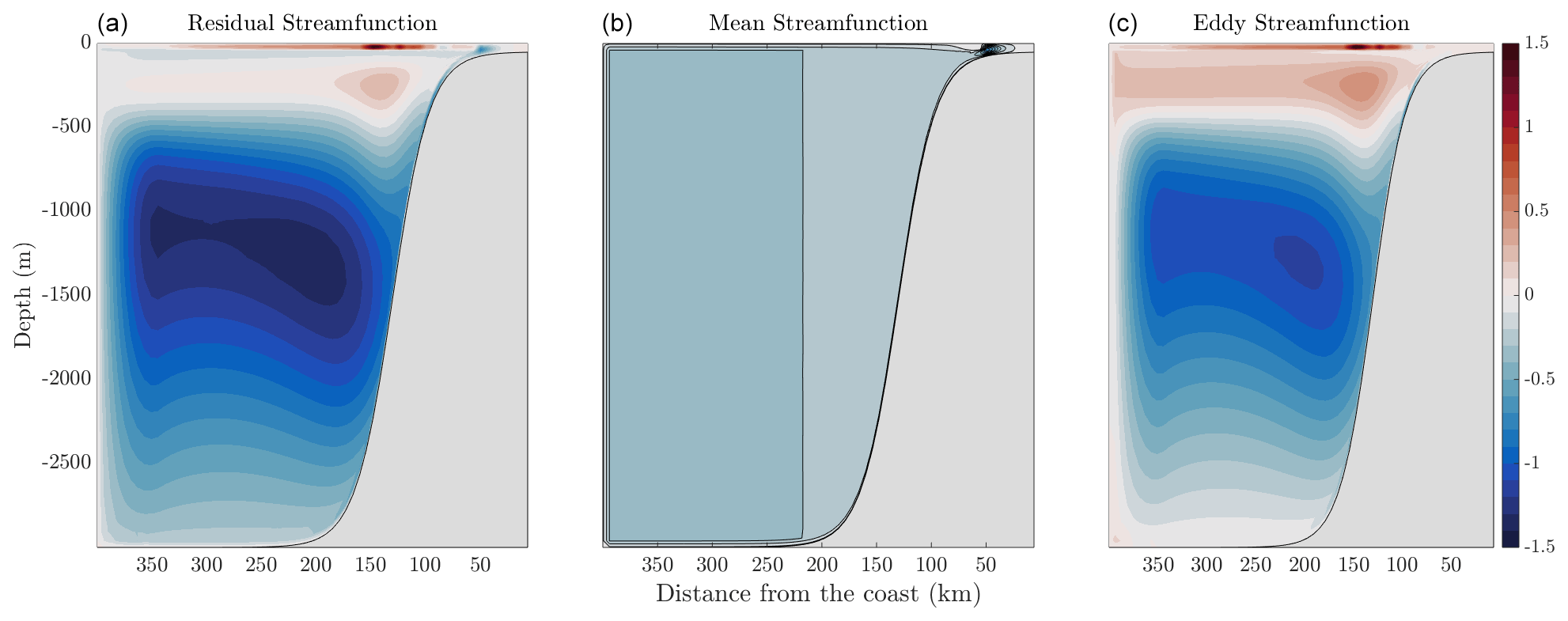
Figure 8Stream functions calculated by MAMEBUS. This figure shows the residual stream function (a) , the mean stream function (b) as calculated in Sect. 2.2, and the eddy stream function (c) as described in Sect. 2.3. Note that positive values indicate clockwise circulation, whereas negative values indicate counter-clockwise circulation.
Table 6A table outlining model run times of varying resolution between a computational cluster comprised of Intel Xeon E5-2650 v3 CPUs and a 2015 Mac laptop running macOS Catalina (version 10.15.7) for 20 model years, for both computing systems, the model is run on a single core. The highest resolution simulation (128×128 horizontal and vertical levels) was conducted on the cluster only due to computational constraints on a laptop.
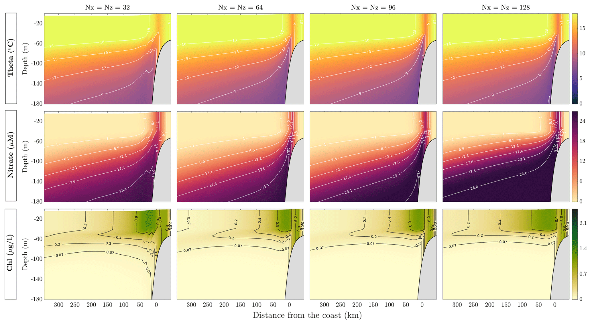
Figure 9This figure shows the model output of temperature, nitrate, and chl with varying resolution. The model was run for 30 years, and solutions shown are averaged over the final 30 years of the model run.
In this paper, we described the formulation, implementation, and main features of MAMEBUS, an idealized, meridionally averaged model of eastern boundary upwelling systems. The solutions are determined by a general evolution equations for materially conserved tracers (Sect. 2) and the fluid momentum equations under the time-dependent turbulent thermal wind (T3W) approximation (Dauhajre and McWilliams, 2018). It includes parameterizations of mesoscale eddy transfer and surface and bottom boundary layer mixing (Sect. 2.3), and a simple ecosystem formulation (Sect. 2.4). We further detailed the algorithms and discretizations implemented in the model (Sect. 3) and discussed reference model inputs and solutions (Sect. 4). Finally, we performed a preliminary validation based on observations from the California Current System, and we discussed the sensitivity of the model to horizontal and vertical resolution (Sect. 5).
MAMEBUS represents a simple, physically consistent tool in which to test and tune a variety of physical parameterizations and ecosystem model formulations. The ultimate goals of this research include exploration of physical–biogeochemical interactions in EBUS, mechanistic understanding of the factors that control cross-shore gradients in biogeochemical and ecological properties, and investigation of the processes that drive differences between distinct EBUSs.
Because of the 2-D framework, we acknowledge shortcomings to the model formulation, including physical aspects like intensification of upwelling around topographic features, for example, resulting from variations in the wind-stress curl (Castelao and Luo, 2018) or fine-scale ocean dynamics. Furthermore, while we parameterize the effect of mesoscale eddies on circulation, we do not account for submesoscale eddies on the shelf, which could play an important role in tracer transport (Dauhajre and McWilliams, 2018). We also do not explicitly represent breaking internal waves and tides on the shelf, which may play an important role in dissipating energy and mixing tracers when the water column is shallow (Lamb, 2014).
In future studies, we plan to use MAMEBUS to explore the effect of physical drivers such as wind stress, bathymetry, stratification, and eddies in controlling the zonal distribution of phytoplankton and food web processes, as informed by a size-structured ecosystem model. Furthermore, we plan to expand upon the physical framework in this paper by expanding eddy parameterizations to include the effect of submesoscale eddies on the shelf, where the mesoscale eddy activity is inhibited. An aspect of MAMEBUS that requires further investigation is the effect of meridional pressure gradients, which we neglected in our reference solutions in Sect. 5. In reality, the presence of along-shore pressure gradients may support interior across-shore transport away from the surface and bottom boundary layers, with the potential to reshape the coastal ecosystem.
With its limited computational cost, MAMEBUS can be used to investigate a wide parameter space in EBUSs and determine their sensitivity to a range of perturbations in major physical forcings, from changes in wind stress to increasing buoyancy forcing associated with climate change (Rykaczewski and Dunne, 2010; Sarmiento et al., 1998). Furthermore, by allowing coupling to a variety of biogeochemical and ecosystem models, MAMEBUS can be used to inform comprehensive regional models (Shchepetkin and McWilliams, 2005), for which computational costs preclude exhaustive sensitivity studies.
In this Appendix, we discuss the partitioning of the mesoscale eddy tracer flux into components due to advection and isopycnal diffusion, used in Sect. 2.1 to derive MAMEBUS's central tracer evolution equation, Eq. (9). We show that the eddy tracer flux, , can be arbitrarily decomposed into components directed along mean buoyancy surfaces and along mean tracer surfaces. These components will later be associated with eddy advection and isopycnal stirring, respectively.
The effect of mesoscale eddies on the averaged tracer concentrations is given by the convergence of the eddy tracer flux (Eq. 8):
and appears on the right-hand side of Eq. (6). Being quasi-adiabatic flows, mesoscale eddies serve to stir material tracers along isopycnal surfaces; this corresponds to an eddy tracer flux directed along buoyancy surfaces (Redi, 1982). Eddies also induce a “bolus” advective transfer of tracers, a generalized “Stokes drift” that corresponds to an eddy tracer flux directed along mean tracer isosurfaces (Gent and McWilliams, 1990). Both of these effects are routinely parameterized in general circulation models (Griffies, 1998, 2018). To partition the eddy tracer flux between isopycnal stirring and bolus advection, we therefore pose a decomposition of into components directed along mean isopycnals and along mean tracer surfaces, respectively:
Here, and are unit vectors that point along mean surfaces and along mean surfaces, respectively:
Note that the x components of and are positive provided that and increase monotonically upward. By taking the vector cross products and , we can solve for the vector lengths αc and αb:
Then, using Eqs. (A2)–(A4), we write Eq. (A1) as
The first term on the right-hand side of Eq. (A5) takes the form of an advection operator, in which we can identify the eddy stream function
Note that this definition is ill-defined in the limit ; in this limit, and are parallel, the eddy tracer flux is purely advective, and the stream function becomes
The second term on the right-hand side of Eq. (A5) has been written in the form of the divergence of a flux along mean buoyancy surfaces, with the isopycnal gradient operator (see Sect. 2.1) appearing explicitly as
We can then identify the isopycnal diffusivity κiso as
where θ is the angle between the vectors and .
While the above derivation is general, for application in MAMEBUS, we must make assumptions about the eddy tracer fluxes. Specifically, we assume (i) that approximately identical eddy stream functions ψ⋆ advect each different model tracer, (ii) that the isopycnal diffusivity is positive (i.e., that eddy tracer fluxes are always directed down the mean tracer gradients), and (iii) that the isopycnal diffusivity is approximately equal for different model tracers. These assumptions are satisfied in the limit of small-amplitude fluctuations (u′ and c′) (Plumb, 1979; Plumb and Ferrari, 2005b).
For a given tracer defined with an associated time tendency equation of the form
We integrate Eq. (B1) in time from :
By the fundamental theorem of calculus,
We interpolate the right-hand side using a Lagrangian polynomial of the form
Then using Eq. (B4) and substituting it into Eq. (B3), we have
Defining , we obtain
Substituting Eq. (B3) into Eq. (B5) yields the full ABII time-stepping scheme, given by Eq. (96).
For higher-order AB methods, we consider a sth-order Lagrangian polynomial of the form
where setting s=3 as the number of known points in the interpolating polynomial results in the ABIII method. Then, s−1 is the degree of the polynomial. The general form of higher-order AB methods is
The algebra to solve for the full discrete form of the ABIII method follows the derivation of the ABII method above. The solution to the integration in Eq. (B8) is given by Eq. (95).
Our representation of eddy advection and isopycnal stirring in the surface mixed layer (SML) and bottom boundary layer (BBL) is adapted from Ferrari et al. (2008) and is described in Sect. 2.3.2. We now directly compare our SML/BBL scheme against that of Ferrari et al. (2008) to highlight the key differences.
As discussed in the “surface mixed layer” subsection, our SML scheme leads to the same eddy stream function as that of Ferrari et al. (2008), given by Eq. (29). In contrast, the residual eddy tracer flux in the SML differs as follows:
where “FMCD” denotes the formulation of Ferrari et al. (2008). Thus, our Eq. (C1b) differs from Eq. (C1a) only by the replacement Sint by Ssml in the vertical eddy residual tracer flux. A drawback of using Sint is that typically the vertical buoyancy gradient is very small in the SML, so the form (Eq. C1a) may not be numerically stable. Ferrari et al. (2008) propose a modification of the vertical component of the tracer residual eddy flux to avoid dividing by small vertical buoyancy gradients in the mixed layer:
However, this alternative breaks the symmetry of the diffusion tensor, and requires the introduction of an additional vertical structure function, . Our formulation, Eq. (C3b), retains the symmetry of the stress tensor and preserves continuity of the vertical flux and its derivative at with the same structure function Gsml(z) (see Sect. 2.3.2). It is also simpler to implement, as both the stream function (Eq. 29) and the residual eddy flux (Eq. C1b) can be written succinctly in terms of the effective slope (Eq. 28).
Another difference between our formulation and that of Ferrari et al. (2008) arises in the eddy stirring of buoyancy in the SML:
The Ferrari et al. (2008) residual eddy buoyancy flux has no vertical component, whereas ours does. This impacts the rate of available potential energy release in the SML by modifying the total vertical eddy buoyancy flux:
The key difference here is that our version (Eq. C4b) typically releases more potential energy and is not strictly positive definite; if , then in principle may be negative. This corresponds to creation of potential energy, whereas previous studies suggest that potential energy should be consistently released in the SML (Colas et al., 2013). However, by construction, the vertical derivative of this term is zero at , and in any practical case will be smaller than throughout the boundary layer. This suggests that if the vertical eddy length scale λ is positive , then our scheme releases potential energy everywhere. Note also that the GM component of the vertical eddy buoyancy flux always releases potential energy.
Finally, we compare the horizontal component of the eddy buoyancy flux in the SML:
Whereas the Ferrari et al. (2008) scheme preserves strict lateral downgradient diffusion, this is only true in our scheme if κgm=κiso.
Further to this comparison with the formulation of Ferrari et al. (2008), we note that the fluxes discussed above differ substantially in the BBL over sloping topography. For example, the vertical buoyancy flux becomes
Thus, in general, the eddy buoyancy flux will act to create potential energy () unless the isopycnal slope Sint is of the same sign as the bottom slope and larger in magnitude. In order to avoid this, it would be necessary to set κiso=0 throughout the BBL. This is a separate consideration from the orientation of the residual flux vector, which must certainly lie parallel to the topography if the diffusivity is nonzero.
The DOI for the MAMEBUS code is https://doi.org/10.5281/zenodo.3866652 (Stewart and Moscoso, 2020).
This package includes the mamebus.c code along with example setup and processing functions that are used in MATLAB.
No data sets were used in this article.
ALS conceived and coordinated the development of MAMEBUSv1.0, and advised JEM in further model development. JEM developed and implemented the ecosystem models, updated the calculation of the momentum equation, and fine-tuned the pressure-gradient calculations. DB coordinated the development of the ecosystem model. JCM coordinated the development of the eddy parameterizations in MAMEBUS and advised JEM in further model development. JEM prepared the manuscript with contributions from all co-authors.
The authors declare that they have no conflict of interest.
This material is based in part upon work supported by the National Science Foundation with grant nos. OCE-1538702, OCE-1751386, and OCE-1635632, and by the National Aeronautics and Space Administration ROSES Physical Oceanography program under grant no. 80NSSC19K1192. Daniele Bianchi gratefully acknowledges funding from the Alfred P. Sloan Foundation. This work used the Extreme Science and Engineering Discovery Environment (XSEDE; Towns et al., 2014), which is supported by National Science Foundation grant no. ACI-1548562.
This research has been supported by the National Science Foundation (grant nos. OCE-1538702, OCE-1751386, OCE-1635632, and ACI-1548562) and the National Aeronautics and Space Administration (grant no. 80NSSC19K1192).
This paper was edited by Qiang Wang and reviewed by two anonymous referees.
Abernathey, R. P. and Marshall, J.: Global surface eddy diffusivities derived from satellite altimetry, J. Geophys. Res.-Oceans, 118, 901–916, 2013. a
Aiki, H. and Richards, K. J.: Energetics of the global ocean: the role of layer-thickness form drag, J. Phys. Oceanogr., 38, 1845–1869, 2008. a
Andersen, K., Berge, T., Gonçalves, R., Hartvig, M., Heuschele, J., Hylander, S., Jacobsen, N., Lindemann, C., Martens, E., Neuheimer, A., Olsson, K., Palacz, A., Prowe, A., Sainmont, J., Traving, S., Visser, A., Wadhwa, N., and Kiørboe, T.: Characteristic Sizes of Life in the Oceans, from Bacteria to Whales, Annu. Rev. Marine Sci., 8, 217–241, 2016. a
Arakawa, A. and Suarez, M. J.: Vertical Differencing of the Primitive Equations in Sigma Coordinates, Mon. Weather Rev., 111, 34–45, 1983. a
Bakun, A. and Nelson, C. S.: The Seasonal Cycle of Wind-Stress Curl in Subtropical Eastern Boundary Current Regions, J. Phys. Oceanogr., 21, 1815–1834, 1991. a
Bakun, A. and Parrish, R. H.: Turbulence, Transport, and Pelagic Fish in the California and Peru Current Systems, CalCOFI Rep., 23, 1982. a
Banas, N. S.: Adding complex trophic interactions to a size-spectral plankton model: Emergent diversity patterns and limits on predictability, Ecol. Modeling, 222, 2663–2675, 2011. a, b, c, d, e, f
Burke, A., Stewart, A. L., Adkins, J. F., Ferrari, R., Jansen, M. F., and Thompson, A. F.: The glacial mid-depth radiocarbon bulge and its implications for the overturning circulation, Paleoceanography, 30, 1021–1039, 2015. a
Cabre, A., Shields, D., Marinov, I., and Kostadinov, T. S.: Phenology of Size-Partitioned Phytoplankton Carbon-Biomass from Ocean Color Remote Sensing and CMIP5 Models, Front. Mar. Sci., 3, 39, 2013. a
Capet, X., Colas, F., McWilliams, J., Penven, P., and Marchesiello, P.: Eddies in eastern boundary subtropical upwelling systems, Ocean Modeling in an Eddying Regime, Geophys. Monogr. Ser, 177, 131–147, 2008. a
Castelao, R. M. and Luo, H.: Upwelling jet separation in the California Current System, Sci. Rep.-UK, 8, 1–8, 2018. a, b
Chavez, F. P. and Messié, M.: A comparison of Eastern Boundary Upwelling Ecosystems, Prog. in Oceanog., 83, 80–96, 2009. a, b, c
Chelton, D. B., DeSzoeke, R. A., Schlax, M. G., El Naggar, K., and Siwertz, N.: Geographical variability of the first baroclinic Rossby radius of deformation, J. Phys. Oceanogr., 28, 433–460, 1998. a
Chenillat, F., Franks, P. J. S., Capet, X., Rivière, P., Grima, N., Blanke, B., and Combes, V.: Eddy properties in the Southern California Current System, Ocean Dynam., 68, 761–777, 2018. a
Colas, F., Capet, X., Mcwilliams, J. C., and Li, Z.: Mesoscale Eddy Buoyancy Flux and Eddy-Induced Circulation in Eastern Boundary Currents, J. Phys. Oc., 43, 1073–1095, 2013. a, b, c
Connolly, T. P., Hickey, B. M., Shulman, I., and Thomson, R. E.: Coastal Trapped Waves, Alongshore Pressure Gradients, and the California Undercurrent, J. Phys. Oceanogr., 44, 319–342, 2014. a, b
Dauhajre, D. P. and McWilliams, J. C.: Diurnal Evolution of Submesoscale Front and Filament Circulations, J. Phys. Oceanogr., 48, 2343–2361, 2018. a, b, c, d, e
Durran, D.: Numerical Methods for Fluid Dynamics: With Applications to Geophysics, Texts in Applied Mathematics, Springer, New York, 2010. a
Durran, D. R.: The third-order Adams-Bashforth method: An attractive alternative to leapfrog time differencing, Mon. Weather Rev., 119, 702–720, 1991. a
Eady, E. T.: Long waves and cyclone waves, Tellus, 1, 33–52, 1949. a
Edwards, A. M. and Bees, M. A.: Generic dynamics of a simple plankton population model with a non-integer exponent of closure, Chaos, Solitons & Fractals, 12, 289–300, 2001. a
Edwards, N. R., Willmott, A. J., and Killworth, P. D.: On the role of topography and wind stress on the stability of the thermohaline circulation, J. Phys. Oceanogr., 28, 756–778, 1998. a
Eto: Data Announcement 88-MGG-02, Digital relief of the Surface of the Earth, 1988. a, b
Ferrari, R., McWilliams, J. C., Canuto, V. M., and Dubovikov, M.: Parameterization of eddy fluxes near oceanic boundaries, J. Climate, 21, 2770–2789, 2008. a, b, c, d, e, f, g, h, i, j, k, l, m, n, o, p, q
Fiechter, J., Edwards, C. A., and Moore, A. M.: Wind, circulation, and topographic effects on alongshore phytoplankton variability in the California Current, Geophys. Res. Lett., 45, 3238–3245, 2018. a, b
Furuya, K.: Subsurface chlorophyll maximum in the tropical and subtropical western Pacific Ocean: Vertical profiles of phytoplankton biomass and its relationship with chlorophylla and particulate organic carbon, Marine Biol., 107, 529–539, 1990. a
Gent, P. R.: The Gent–McWilliams parameterization: 20/20 hindsight, Ocean Modell., 39, 2–9, 2011. a
Gent, P. R. and McWilliams, J. C.: Isopycnal mixing in ocean circulation models, J. Phys. Oceanogr., 20, 150–155, 1990. a, b, c, d
Griffies, S.: Fundamentals of ocean climate models, Princeton University Press, 2018. a, b, c
Griffies, S. M.: The Gent–McWilliams skew flux, J. Phys. Oceanogr., 28, 831–841, 1998. a
Gruber, N., Lachkar, Z., Frenzel, H., Marchesiello, P., Münnich, M., McWilliams, J. C., Nagai, T., and Plattner, G.-K.: Eddy-induced reduction of biological production in eastern boundary upwelling systems, Nat. Geosci., 4, 787–792, 2011. a, b
Gula, J., Molemaker, M. J., and McWilliams, J. C.: Submesoscale cold filaments in the Gulf Stream, J. Phys. Oceanogr., 44, 2617–2643, 2014. a
Haney, R. L.: Surface thermal boundary condition for ocean circulation models, J. Phys. Oceanogr., 1, 241–248, 1971. a
Haney, R. L.: On the Pressure Gradient Force over Steep Topography in Sigma Coordinate Ocean Models, J. Phys. Oceanogr., 21, 610–619, 1991. a
Hansen, B., Bjornsen, P., and Hansen, P.: The size ratio between planktonic predators and their prey, Limnol. Oceanogr., 39, 395–403, 1994. a, b, c, d
Jacox, M. and Edwards, C.: Effects of stratification and shelf slope on nutrient supply in coastal upwelling regions, J. Geophys. Res.-Oceans, 116, C3, 2011. a
Jacox, M. and Edwards, C.: Upwelling source depth in the presence of nearshore wind stress curl, J. Phys. Resc., 117, C5, 2012. a, b, c
Jacox, M. G., Moore, A. M., Edwards, C. A., and Fiechter, J.: Spatially resolved upwelling in the California Current System and its connections to climate variability, Geophys. Res. Lett., 41, 3189–3196, 2014. a
Kahan, W.: Pracniques: further remarks on reducing truncation errors, Communications of the ACM, 8, 40, 1965. a
Kays, W. M.: Turbulent Prandtl number. Where are we?, ASME Transactions J. Heat Transf., 116, 284–295, 1994. a
Kurganov, A. and Tadmor, E.: New high-resolution central schemes for nonlinear conservation laws and convection-diffusion equations, J. Comput. Phys., 160, 241–282, 2000. a, b, c, d
Lamb, K. G.: Internal Wave Breaking and Dissipation Mechanisms on the Continental Slope/Shelf, Annu. Rev. Fluid Mech., 46, 231–254, 2014. a
Large, W. G., McWilliams, J. C., and Doney, S. C.: Oceanic vertical mixing: A review and a model with a nonlocal boundary layer parameterization, Rev. Geophys., 32, 363–403, 1994. a, b
Lentz, S. J. and Chapman, D. C.: The importance of nonlinear cross-shelf momentum flux during wind-driven coastal upwelling, J. Phys. Oceanogr., 34, 2444–2457, 2004. a
Lentz, S. J. and Fewings, M. R.: The wind-and wave-driven inner-shelf circulation, Annu. Rev. Marine Sci., 4, 317–343, 2012. a
MATLAB: version 9.1.0 (R2016b), The MathWorks Inc., Natick, Massachusetts, 2016. a
McClatchie, S.: Regional fisheries oceanography of the California Current System, Springer, 2016. a, b, c, d
McDougall, T. J. and Ferrari, R.: Abyssal upwelling and downwelling driven by near-boundary mixing, J. Phys. Oceanogr., 47, 261–283, 2017. a
Mellor, G. L., Ezer, T., and Oey, L.-Y.: The Pressure Gradient Conundrum of Sigma Coordinate Ocean Models, J. Atmos. Ocean. Tech., 11, 1126–1134, 1994. a
Mellor, G. L., Oey, L.-Y., and Ezer, T.: Sigma Coordinate Pressure Gradient Errors and the Seamount Problem, J. Atmos. Ocean. Tech., 15, 1122–1131, 1998. a
Moore, J., Doney, S. C., Kleypas, J. A., Glover, D. M., and Fung, I. Y.: An intermediate complexity marine ecosystem model for the global domain, Deep-Sea Res., 49, 403–462, 2001. a, b, c, d, e
Plumb, R. A.: Eddy fluxes of conserved quantities by small-amplitude waves, J. Atmos. Sci., 36, 1699–1704, 1979. a, b
Plumb, R. A. and Ferrari, R.: Transformed Eulerian-Mean Theory. Part I: Nonquasigeostrophic Theory for Eddies on a Zonal-Mean Flow, J. Phys. Oceanogr., 35, 165–174, 2005a. a
Plumb, R. A. and Ferrari, R.: Transformed Eulerian-mean theory. Part I: Nonquasigeostrophic theory for eddies on a zonal-mean flow, J. Phys. Oceanogr., 35, 165–174, 2005b. a, b
Poulin, F. J. and Franks, P. J. S.: Size-Structured planktonic ecosystems: constraints, controls, and assembly instructions, J. Plankton Res., 32, 1121–1130, 2010. a, b
Raick, C., Soetaert, K., and Gregoire, M.: Model complexity and performance: How far can we simplify?, Prog. Oceanogr., 70, 27–57, 2006. a
Redi, M. H.: Oceanic isopycnal mixing by coordinate rotation, J. Phys. Oceanogr., 12, 1154–1158, 1982. a, b, c, d
Renault, L., Deutsch, C., McWilliams, J., Frenzel, H., Liang, J., and Colas, F.: Partial decoupling of primary productivity from upwelling in the California Current system, Nat. Geo. Sci., 9, 505–510, 2016. a, b
Rykaczewski, R. R. and Dunne, J. P.: Enhanced nutrient supply to the California Current Ecosystem with global warming and increased stratification in an earth system model, Geophys. Res. Lett., 37, 21, 2010. a, b
Sarmiento, J. L. and Gruber, N.: Ocean Biogeochemical Dynamics, Princeton University Press, 2006. a, b, c, d, e
Sarmiento, J. L., Hughes, T. M. C., Stouffer, R. J., and Manabe, S.: Simulated response of the ocean carbon cycle to anthropogenic climate warming, Lett. Nature, 393, 245–249, 1998. a
Shchepetkin, A. F. and McWilliams, J. C.: A method for computing horizontal pressure-gradient force in an oceanic model with a nonaligned vertical coordinate, J. Geophys. Res.-Oceans, 108, C3, 2003. a, b, c, d, e, f, g, h, i, j, k
Shchepetkin, A. F. and McWilliams, J. C.: The Regional Ocean Modeling System: A split-explicit, free-surface, topography following coordinates ocean model, Ocean Modell., 9, 347–404, 2005. a, b, c, d
Smith, K. S. and Marshall, J.: Evidence for Enhanced Eddy Mixing at Middepth in the Southern Ocean, J. Phys. Oceanogr., 39, 50–69, 2009. a
Song, Y. and Haidvogel, D.: A semi-implicit ocean circulation model using a generalized topography-following coordinate system, J. Comput. Phys., 115, 228–244, 1994. a, b, c
Stewart, A. L. and Moscoso, J. E.: A Meridionally Averaged Model of Eastern Boundary Upwelling Systems (v1.0) (Version v1.0), Zenodo, https://doi.org/10.5281/zenodo.3866652, 2020. a
St. Laurent, L., Simmons, H., and Jayne, S.: Estimating tidally driven mixing in the deep ocean, Geophys. Res. Lett., 29, 21–1, 2002. a
Tang, E.: The allometry of algal growth rates, Journal of Plankton Research, 17, 1325–1335, 1995. a, b
Towns, J., Cockerill, T., Dahan, M., Foster, I., Gaither, K., Grimshaw, A., Hazlewood, V., Lathrop, S., Lifka, D., Peterson, G. D., Roskies, R., Scott, J. R., and Wilkins-Diehr, N.: XSEDE: accelerating scientific discovery, Comput. Sci. Eng., 16, 62–74, 2014. a
Tréguier, A.-M., Held, I. M., and Larichev, V. D.: Parameterization of quasigeostrophic eddies in primitive equation ocean models, J. Phys. Oceanogr., 27, 567–580, 1997. a
Troen, I. B. and Mahrt, L.: A simple model of the atmospheric boundary layer; sensitivity to surface evaporation, Bound.-Lay. Meteorol., 37, 129–148, 1986. a
Vallis, G. K.: Atmospheric and oceanic fluid dynamics, Cambridge University Press, 2017. a, b, c
Van Oostende, N., Dussin, R., Stock, C., Barton, A., Curchitser, E., Dunne, J., and Ward, B.: Simulating the ocean's chlorophyll dynamic range from coastal upwelling to oligotrophy, Prog. Oceanogr., 168, 232–247, 2018. a
Venegas, R. M., Strub, P. T., Beier, E., Letelier, R., Thomas, A. C., Cowles, T., James, C., Soto-Mardones, L., and Cabrera, C.: Satellite-derived variability in chlorophyll, wind stress, sea surface height, and temperature in the northern California Current System, J. Geophys. Res.-Oceans, 113, C3, 2008. a
Wang, Y. and Stewart, A. L.: Eddy dynamics over continental slopes under retrograde winds: Insights from a model inter-comparison, Ocean Modell., 121, 1–18, 2018. a
Wang, Y. and Stewart, A. L.: Scalings for eddy buoyancy transfer across continental slopes under retrograde winds, Ocean Modell., 147, 101579, https://doi.org/10.1016/j.ocemod.2020.101579, 2020. a
Ward, B. A., Dutkiewicz, S., Jahn, O., and Follows, M. J.: A size-structured food-web model for the global ocean, Limnol. Oceanogr., 57, 1877–1891, 2012. a, b, c
- Abstract
- Introduction
- MAMEBUS framework
- MAMEBUSv1.0 algorithm
- Implementation details
- Reference solution and model validation
- Discussion and future work
- Appendix A: Decomposing mesoscale eddy advective/diffusive fluxes
- Appendix B: Derivation of time-variable Adams–Bashforth methods
- Appendix C: Comparison of boundary layer parameterizations with Ferrari et al. (2008)
- Code availability
- Data availability
- Author contributions
- Competing interests
- Acknowledgements
- Financial support
- Review statement
- References