the Creative Commons Attribution 4.0 License.
the Creative Commons Attribution 4.0 License.
 | 08 Dec 2021
SELF v1.0: a minimal physical model for predicting time of freeze-up in lakes
Luca Cortese
Predicting the freezing time in lakes is achieved by means of complex mechanistic models or by simplified statistical regressions considering integral quantities. Here, we propose a minimal model (SELF) built on sound physical grounds that focuses on the pre-freezing period that goes from mixed conditions (lake temperature at 4 ∘C) to the formation of ice (0 ∘C at the surface) in dimictic lakes. The model is based on the energy balance involving the two main processes governing the inverse stratification dynamics: cooling of water due to heat loss and wind-driven mixing of the surface layer. They play opposite roles in determining the time required for ice formation and contribute to the large interannual variability observed in ice phenology. More intense cooling does indeed accelerate the rate of decrease of lake surface water temperature (LSWT), while stronger wind deepens the surface layer, increasing the heat capacity and thus reducing the rate of decrease of LSWT. A statistical characterization of the process is obtained with a Monte Carlo simulation considering random sequences of the energy fluxes. The results, interpreted through an approximate analytical solution of the minimal model, elucidate the general tendency of the system, suggesting a power law dependence of the pre-freezing duration on the energy fluxes. This simple yet physically based model is characterized by a single calibration parameter, the efficiency of the wind energy transfer to the change of potential energy in the lake. Thus, SELF can be used as a prognostic tool for the phenology of lake freezing.
- Article
(2039 KB) - Full-text XML
-
Supplement
(2590 KB) - BibTeX
- EndNote


Lake ice phenology is listed as an essential climate product by the global climate observing system. Long-term trends in lake ice phenology are indeed robust archives for climate changes and delays in the calendar dates of the freezing process and earlier thawing are well documented (Livingstone, 1997; Magnuson, 2000; Livingstone et al., 2010; Leppäranta, 2015). While long-term trends regarding the decrease in ice duration are clear, ice phenology time series are also characterized by strong interannual variability (Magnuson, 2000) making any short-term prediction of the ice duration challenging.
The freezing time depends on the amount of heat that was stored in the lake during the summertime and the following rate of heat extraction in fall and winter. Both competing processes are driven by atmospheric forcing. If we exclude very deep lakes, where thermobaric instabilities can increase the complexity of the process, the different phases can be described as follows. First, the combination of atmospheric cooling and mechanical wind energy extracts the heat stored in the warm stratified surface layer and progressively deepens the surface layer to the lake bottom, until the lake reaches homothermal conditions. Neglecting salinity and pressure effects on density, the homothermal condition is necessarily satisfied when the lake surface water temperature, Ts, is equal to the temperature of maximal density, here set at Tmd = 4 ∘C. The dynamics of the pre-freezing period, here defined as the time when 0 < Ts < Tmd, change compared to the preceding period. Indeed, in the pre-freezing period, the timing of ice formation is driven by a competition between stabilizing cooling processes (negative heat flux resulting from seasonal decline in solar radiation, which can be correlated also to air temperature, Ta, being colder than lake temperature) and destabilizing processes (mainly wind). The exact freezing time, occurring when a thin layer at the surface reaches 0 ∘C with a stable temperature gradient below, is dominated by the contribution of the air temperature in the non-penetrative heat flux. However, both penetrative radiation and wind stress can balance the non-penetrative heat flux by mixing the previously stratified surface layer, thereby delaying ice formation. Said differently, the interaction between the different forcing terms (i.e., wind stress and air temperature) will determine the amount of heat to be extracted before the lake begins to freeze.
The modern approach to predict freezing time consists of using one-dimensional (1D) hydrodynamic models (Liston and Hall, 1995; Duguay et al., 2003; Dibike et al., 2011; MacKay et al., 2017; Hipsey et al., 2019; Gaudard et al., 2019) coupled with an ice module (Leppäranta, 1993). Such models can be used in prognostic mode but require a large amount of information to be measured near the lake to resolve the heat budget. Hence, it remains challenging to accurately estimate ice phenology in lakes at global scale based on such deterministic models.
The alternative approach, historically initiated in the first part of the 20th century, consists of simplifying the problem by assuming that air temperature is the main driver for ice formation. The heat flux can then be linearized and takes the form of a first-order differential equation with the lag term (or reaction term) being a function of the mixed layer depth (Leppäranta, 2014). Given negative air temperature as necessary condition for lake freezing, ice formation was further predicted by an integration of negative degree days (Bilello, 1964). This approach was extended by Franssen and Scherrer (2008) with the addition of the mean lake depth as a secondary explanatory variable for ice formation in Swiss lakes. However, uncertainties related to this integral approach have been already discussed by Rodhe (1952), who developed a relationship between weighted air temperatures and ice formation over the cooling period. Weyhenmeyer et al. (2011) proposed an approach that takes into account the temporal evolution of the air temperature, Ta. However, all those models are intrinsically based on the assumption that the interannual variability of other parameters contributing to the heat budget remain small compared to the change in Ta or covary with Ta. The temporal competition between stabilizing and destabilizing factors in the pre-freezing phase are thereby not explicitly accounted for in most statistical models.
In this study, we develop a minimal model to predict the time of ice formation based on time series of meteorological variables. It is important to note that we focus only on the pre-freezing period, i.e., from the day in which the lake is completely mixed (homothermal) to the day when the surface temperature drops to 0 ∘C. First, we test the model against the results of a 1D numerical model, Simstrat (Goudsmit et al., 2002; Gaudard et al., 2019), calibrated with in situ observations for five Swiss lakes, and then we exploit the simple structure of the minimal model to infer some statistical properties of the freezing process.
2.1 Phenomenological description
The minimal model (Stratification Energy before Lake Freezing – SELF) simulates the two main processes affecting the development of inverse stratification in the pre-freezing period: the loss of thermal energy due to atmospheric cooling and the input of mechanical energy due to wind stress on the lake surface. The separation of the two processes over a relevant timescale is the core of the minimal model. First, we describe it qualitatively, and then we formulate the mathematical model in the following section. Further details about the simplification of the energy balance are discussed in the Supplement.
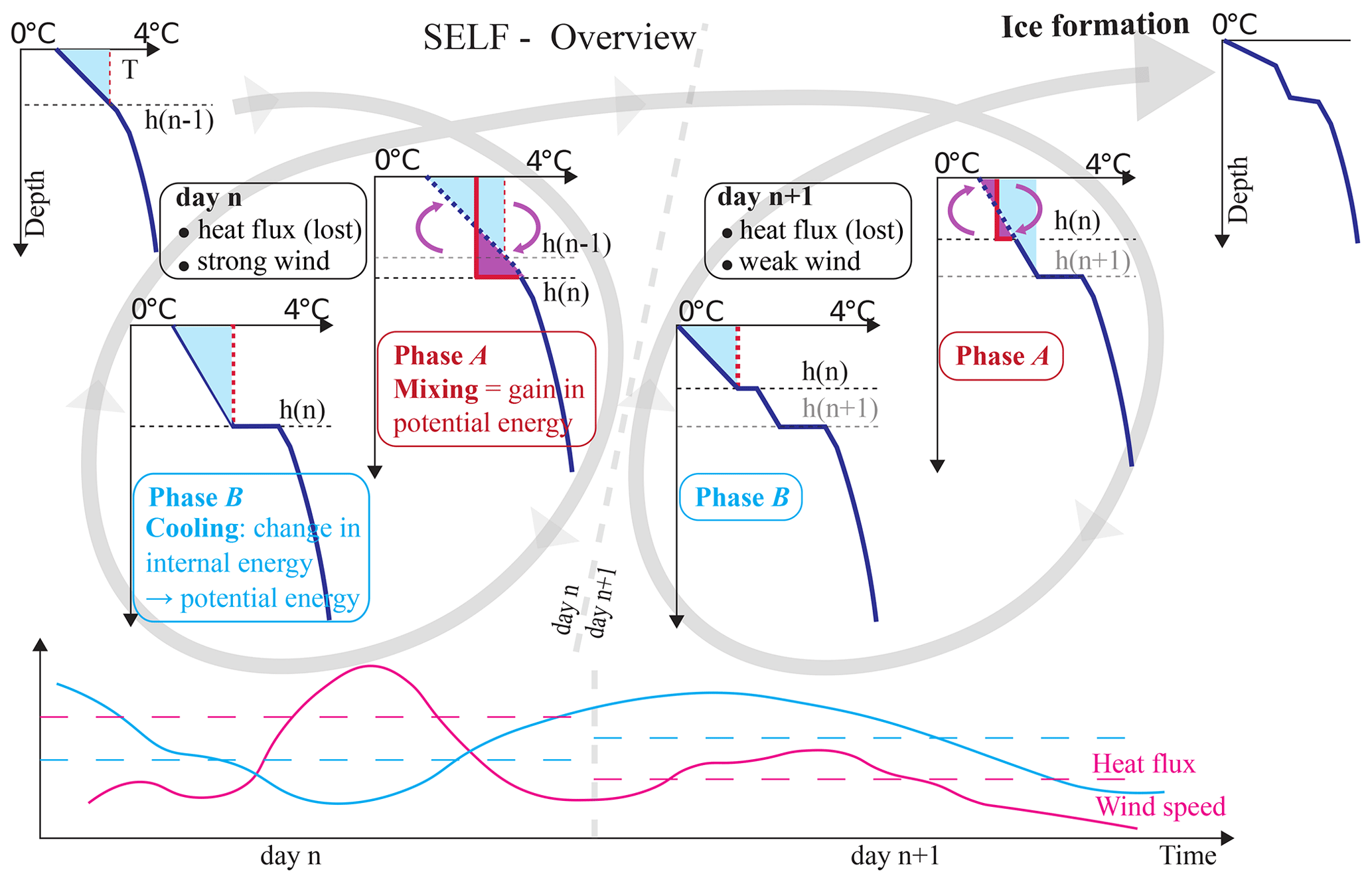
Figure 1Conceptual sketch of the minimal model describing the main processes in the pre-freezing period. Starting from stratified initial conditions (T profile on the top left) at day n, part of the wind energy is used to mix the surface layer (phase A). This step sets the thickness of the surface layer, which stratifies due to the heat loss (phase B). The two phases are repeated for day n+1 until the wind stress becomes low enough (reducing the thickness of the surface layer) and the cooling strong enough that the temperature at the surface may drop below 0 ∘C, thus forming an ice sheet. The resulting T profile (on the right) tends to become curved (with a concave shape) because the surface layer becomes thinner on average when the stratification is stronger.
The evolution of the stratification modeled by SELF is illustrated in Fig. 1. Starting from a stratified water column, the wind stress provides an amount of mechanical energy that mixes the surface layer (phase A), making the temperature uniform and conserving the thermal energy. The layer's thickness h is determined by balancing the change of potential energy and the fraction of the mechanical energy that is effectively transferred by the wind during a suitably chosen timescale Δt. The second step (phase B) describes the variation of water temperature distribution due to the net heat flux: we assume that the surface layer stratifies following an approximately linear profile of temperature along h. When heat is lost, the surface layer stably stratifies because water cools progressively from the free surface downwards. When water at the surface warms but remains below 4 ∘C, the stratification is instead unstable due to convective overturn and is readily mixed in the subsequent phase A. The cycle iterates until ice forms at the surface; this typically occurs for weak wind conditions when the surface temperature is cold enough. Note that the sequence of mixing and cooling phases, with the surface layer thickness progressively decreasing, gradually builds up a temperature profile with a concave shape, as will be shown later.
A natural choice for the time step of the proposed model is to consider the energy fluxes integrated over a daily cycle (Δt = 86 400 s, 1 d). This retains the net effect of the heat fluxes that are characterized by the diel periodicity given by the solar radiation input. On the other hand, this also means that the destabilizing effect of surface warming during the warmest hours of the day is not explicitly considered in this model.
The net heat flux exchanged through the lake free surface is computed as the sum of several components [W m−2]:
where the terms on the right-hand side are, respectively, the downward shortwave radiation, the downward longwave (infrared) radiation (mostly depending on air temperature, Ta, and cloud cover), the longwave radiation emitted from the lake (depending only on lake surface water temperature, LSWT, Ts), the sensible (convection) heat flux (depending on the difference between Ts and Ta through an exchange coefficient that is a function of the wind speed W), and the latent (evaporation, condensation) heat flux (eventually depending on Ts, Ta, and W). All of these terms are evaluated using the same empirical relations implemented in Simstrat (Goudsmit et al., 2002).
In order to keep the model simple, we consider the whole shortwave radiation input to the lake in the computation of the net heat flux (Eq. 1) without distinguishing the fraction that is actually absorbed from the surface layer of thickness h from the fraction that penetrates deeper. This assumption might be inaccurate when the surface layer is shallower than the inverse of the extinction coefficient.
2.2 Mathematical formulation
In this section we formulate the model, which we test against observations and numerical results in the next section. We consider a water column of unit area with variable density ρ(z,t) [kg m−3] and temperature T(z,t) [∘C], linked via a nonlinear equation of state, in a gravitational field with acceleration g [m s−2], where z [m] is the vertical coordinate pointing downwards. The minimal model computes (i) over which depth the previously stratified water column will be mixed (phase A) and (ii) the final temperature profile in the newly created mixed layer after cooling has caused stabilizing conditions (phase B). The equation of state was simplified by neglecting the effect of pressure and salinity, hence ρ(z)=ρ(T(z)), and calibrating the coefficients of a parabolic function of T between 0 and 4 ∘C:
where the coefficients a0=999.8683 kg m−3, a1=0.0662498 , and were obtained from a quadratic regression of a widely used relation (Martin and McCutcheon, 1999; Read et al., 2011) with root-mean-square error kg m−3, bias kg m−3, and respecting that Tmd=3.986 ∘C.
If not otherwise specified, we assume that the volume of the lake is conserved even when the density changes. Although this assumption is physically incorrect (mass is conserved, not volume), it is routinely adopted in all practically used numerical models and does not significantly affect the final results (for a deeper discussion, see the Supplement).
We start analyzing the processes in phase A. At a given time t, the potential energy per unit area [J m−2] is computed from the free surface (z=0) to a generic depth Z:
In a well-mixed surface layer of thickness h, with uniform temperature and density ρm=ρ(Tm), the potential energy is . Hence, the change of potential energy from a stratified condition to a well-mixed layer (for the same depth h) is . The demonstration of the latter inequality is given in the Supplement.
The energy required to mix the layer down to a depth h comes from the wind force acting on the lake surface. However, only a small fraction of the wind energy is actually transferred into the change of potential energy ΔEp(h), and most of it is eventually dissipated. The estimation of the effective wind energy can be split into two processes: (i) the energy transferred from the wind to the surface currents and (ii) the transfer of the kinetic energy into the change of potential energy of the water column.
Concerning the first process, the wind power [W m−2] is usually estimated as
where τ [N m−2] is the wind shear stress on the lake surface, W [m s−1] is the wind speed, ρa is the air density, and CD [–] is the wind-dependent drag coefficient. By integrating the wind power over a day, we obtain the wind energy Ew = ∫ΔtPwdt []. A fraction of this energy is transferred to the lake in terms of mechanical work Ek = ∫ΔtτUdt [] that increases the kinetic energy of the wind-driven currents at the lake surface, where U [m s−1] is the surface water velocity (precisely, its component in the direction of the wind). Here, we introduce a first efficiency factor as Ek=η1Ew. A preliminary estimate of this ratio, based on the dependence of U on W, is provided in the Supplement. We note that the definition of Ew is not unequivocal since it depends on the height where the wind speed is measured but has the advantage of being simple; conversely, the definition of Ek is rigorous but the velocity U is more difficult to estimate properly.
Following this, we focus on the second process, i.e., the transfer of the kinetic energy into the change of potential energy of the water column. Only a fraction of the whole kinetic energy Ek is transformed into potential energy of the water column (Kullenberg, 1976). A large fraction is dissipated due to internal friction (turbulence and eventually viscous dissipation at the small scales), and another fraction is used to accelerate the flow in the well-mixed layer (possibly considering also the entrainment of calm water if the layer becomes deeper). The remaining effect is quantified through a second efficiency as ΔEp=η2Ek. All basin-scale dynamic phenomena (upwelling and downwelling, seiches, and so on) eventually contribute to this term.
It is complicated to provide an independent quantification of the two coefficients η1 and η2 exactly. Instead, we refer to a single calibration parameter in the form of the global efficiency η of the energy transfer from the wind to the change of potential energy in the lake, such that
where η=η1η2. Thus, given the wind energy, it is possible to compute the depth h of the surface layer that is mixed due to the wind action.
The formation of the stratification (phase B) is also difficult to characterize in simple terms because it depends on how the temperature changes with depth: the vertical (turbulent in many cases) diffusion of heat interacts with the penetration of shortwave radiation and the convective flux. In our simplified model, as a first approximation we assume that a linear temperature profile develops in the well-mixed layer h, with the temperature unchanged at the depth h and the largest variability at the surface. The net heat flux across the free surface (assumed positive for cooling, when the flux is directed from the lake to the atmosphere) includes the incoming shortwave radiation and the other heat fluxes exchanged with the atmosphere. The energy per unit area Ec exchanged during the interval Δt [] is computed by integrating the net heat flux in time, Ec = ∫ΔtHnetdt.
Given the thickness h of the surface layer and the heat loss Ec, the assumed linear temperature profile establishes a relation Ec = , where ρ0 is a reference value for water density. Thus, it is possible to compute the difference between the undisturbed temperature at the bottom of the layer, T|z=h, and that at the surface, ,
Hence, the change in the T profile modifies the potential energy of the system (phase B in Fig. 1), leading to a condition where an input of external energy (wind) is required to mix it again.
2.3 Cumulated energy and duration of the pre-freezing period
Having presented the minimal model, we focus then on the expected output. We define as nd the number of days between the start of the simulation (on the day when Ts permanently falls below Tmd) and the first time when Ts < 0 ∘C, i.e., the duration of the inverse stratification (pre-freezing) period. Referring to this period, we define the cumulative values [J m−2] of the mechanical and thermal energy as follows:
Moreover, we are going to relate our results with other approaches based on negative degree days, D [∘C d], defined as follows:
where Ta is the daily averaged air temperature (expressed in ∘C). The summation is done only for values of Ta < 0 ∘C (Franssen and Scherrer, 2008).
2.4 Approximate explicit solution
The set of equations that defines the model SELF does not admit an analytical solution in explicit form, for instance in terms of a relation for the number of days nd as a function of the forcing variables. However, a simplified explicit dependence between and can be obtained only by introducing other additional assumptions that are not fully realistic. Bearing in mind that the obtained solution does not aim to describe real conditions but instead to explore the relative contribution of heat loss and wind intensity, we assume that the daily energy fluxes are constant (and hence neglect the history of the system) and that the density depends linearly on T (not representative of what occurs in the range 0–4 ∘C, as already noted). Referring the reader to the derivation provided in the Supplement for the details, an approximate quadratic dependence between the cumulated energies is obtained:
with the proportionality coefficient s2 kg−1. The very small value of the coefficient k is due to the several orders of magnitude of difference between the heat loss, , and the mixing energy, , amplified by the quadratic dependence.
The approximate analytical solution also provides a direct estimate of the duration of the pre-freezing period,
as a function of the averaged daily values of the energy (indicated by angle brackets). Although there are unrealistic simplifications introduced to derive such a result, Eqs. (10) and (11) provide a way to interpret the relationship between the strengths of cooling and wind mixing. This solution corresponds to an extension of the well-established estimate of ice freezing probability based on negative degree day. Specifically, the term expressing heat loss is an analog to the negative degree day, while the addition of a term expressing the mixing energy now includes the delaying effect of wind intensity.
3.1 Observations
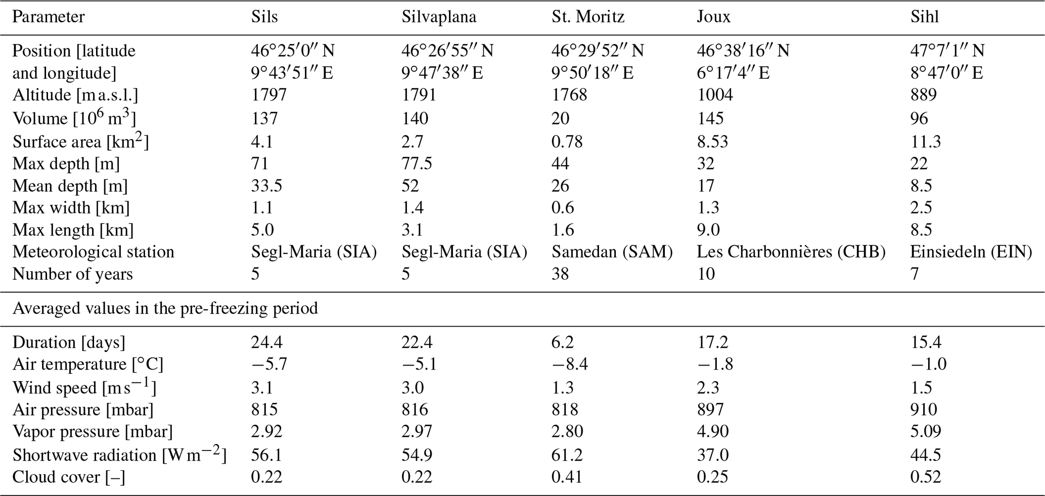
Five Swiss lakes were selected as case studies: Sils, Silvaplana, St. Moritz, Sihl, and Joux. The main relevant geographical and meteorological characteristics are provided in Table 1. Those five lakes cover a wide range of different forcing conditions in the pre-freezing period, varying from mild to cold air temperature and weak to moderate wind intensities (see also the analysis in the Results section). For each lake, wind speed, air temperature, incoming solar radiation, vapor pressure, and cloud cover data were taken from the closest meteorological station within the automatic monitoring network of MeteoSwiss (see Table 1).
Table 1Main geographical and meteorological characteristics of the studied lakes.
Lake temperatures are continuously recorded at different depths. For Lake Joux, the mooring consists of 9 temperature loggers (accuracy 0.1 ∘C) equally spaced from 2 m below the surface to the lake bottom; the monitoring system has been in place since 2013. For Lakes Sils, Silvaplana, St. Moritz, and Sihl, the moorings consist of 11 temperature loggers (accuracy 0.1 ∘C). In the first year (2016), the mooring was designed to follow the evolution of the temperature in the surface layer with the first temperature logger ∼ 5 cm below the surface. The distance to the next sensor was set to be the double of the distance just above. For safety and practical issues, the mooring stopped at a sub-surface buoy 2 m below the surface in the following years.
These datasets provide the necessary information to validate a 1D hydrodynamic model for standard applications related to the evolution of the thermal structure. However, in this case, where we aim to consider the LSWT, the distance of the logger closest to the surface is not sufficient to obtain information about the correct timing of ice formation and hence to robustly validate our minimal model. For this reason, a traditional physically based model (which provides the water temperature right at the lake surface) was used as the prototype to compare with.
3.2 One-dimensional full model
We used a 1D vertical hydrodynamic model, Simstrat v2.1 (Gaudard et al., 2019), to provide a vertically resolved time series of water temperatures for testing the proposed minimal model. For details about the model structure, we refer the reader to Goudsmit et al. (2002). Here it suffices to mention that the heat fluxes are calculated in the same way as for the minimal model (Eq. 1); note that this method does not take the atmospheric stability into account. Similarly, wind energy transferred to the lake is estimated with the same wind drag coefficient (Wüest and Lorke, 2003) used in SELF.
Simstrat has already been successfully applied to the five investigated lakes for yearly monitoring of the thermal structure (Gaudard et al., 2019). Here, we specifically calibrated Simstrat to the pre-freezing period. For each lake, the calibration parameters were adjusted based on the first year of observations, and the model was validated with the following pre-freezing periods (more details about the performance in the Supplement). The beginning of the pre-freezing period was defined at the time that the upper temperature logger reached 4 ∘C.
We acknowledge that even the one-dimensional approach of the mechanistic model cannot accurately reproduce the exact timing of ice formation given the horizontal variability of the ice formation process at the lake surface, typically starting from the shore and propagating offshore over a couple of days (Leppäranta, 2015). Nevertheless, in the absence of detailed information about the spatial distribution of ice in the majority of lakes, 1D models often represent the only deterministic approach consistent with the knowledge available for the investigated system. In this respect, SELF contains an even more simplified description of the vertical stratification process with regard to classical physically based models such as Simstrat.
3.3 Calibration of the minimal model
In order to calibrate the wind-to-potential-energy efficiency η in the minimal model, we compared the results of SELF with those obtained with Simstrat. The following two aspects were considered: the duration of the pre-freezing period, nd, and the difference in daily LSWT, Ts, during this period. We weighted the two factors to define the error to be minimized:
where and ωT = 1 is the (arbitrarily chosen) relative weight of the temperature deviation during the simulation period with respect to the freezing time difference. The optimal value of the parameter η was obtained by minimizing err for each lake using a bifurcation algorithm.
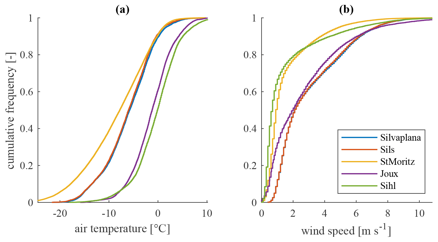
Figure 2Comparison of the meteorological conditions among the five lakes: cumulative distribution of air temperature (a) and wind speed (b) in the extended (i.e., considering 15 d after the latest ice-on date for each lake) pre-freezing period, computed using the whole series of available measurements (see Table 1). The distributions are plotted between the values 0.01 and 0.99 of cumulative frequency. Note that the data of Lakes Silvaplana and Sils are almost coincident because they refer to the same meteorological station and the only difference lies in the slightly different duration of the pre-freezing period in the two lakes.
4.1 Climatological characterization of the pre-freezing period
In this section, we present the statistics of the wind speed and air temperature, considered the main meteorological drivers of lake freezing, for the five selected Swiss lakes. Our analysis focuses on the pre-freezing period, which we extend for each lake from the day of homothermal conditions (in each year, the latest date when LSWT drops below 4 ∘C) to 15 d after the latest date of ice cover formation in the available results (hereafter, this period will be qualified as “extended”). The cumulative distributions of air temperature and wind speed shown in Fig. 2 indicate a wide range of forcing conditions, although the five lakes lie in similar geographical region.
The two lakes that are located around approximately 1000 (above sea level), Lake Sihl and Lake Joux, have a median air temperature of −1.0 and −1.8 ∘C over the extended pre-freezing period, respectively. Air temperature in the higher-altitude lakes (∼ 1700 ) is almost constantly below zero in the same period, with median air temperature of −8.4 ∘C for Lake St. Moritz and −5.7 and −5.1 ∘C for Lakes Silvaplana and Sils (Fig. 2a). Note that for the last two lakes there is only one meteorological station, and the median air temperature depends on the extended pre-freezing averaging window, which differs between lakes. From these results, we expect nd to be longer for Lakes Joux and Sihl and likely the shortest for Lake St. Moritz. Wind intensity also varies over the investigated system, with median wind speed and wind power being, respectively, 2 and 8 times stronger (wind power depending on the third power of wind speed) over Lakes Joux, Silvaplana, and Sils than over Lakes St. Moritz and Sihl (Fig. 2b). When adding wind information, we now expect Lake Sihl to have a shorter nd than Lake de Joux and similarly expect Lake St. Moritz to have the shortest nd over the Upper Engadine lakes. The large range in the observed forcing allows for future global application of our regional process-based study.
4.2 Performance of Simstrat
We compare the temperatures simulated with Simstrat and the different near-surface temperature loggers during the pre-freezing period (Fig. 3a). The model performances are summarized with an R2 of 0.88 and RMSE (root-mean-square error) of 0.19 ∘C. From Fig. 3a, where the data become very sparse for LSWT close to 0 ∘C because the logger is not at the surface, we immediately see that we lack information near the surface, which is needed to calibrate SELF in a proper way. In 2016, the loggers installed near the surface in Lake Sihl could measure the temporal evolution of this layer down to a temperature of 0.5 ∘C (Fig. 3b). The simulated temperatures with Simstrat follows the general trend with a RMSE = 0.23 ∘C. Interestingly, the change in slope at the end of the period is correctly reproduced by the model. This evidence further supports the use of Simstrat to simulate the evolution of the thermal structure during the pre-freezing period.

Figure 3Performance of Simstrat in reproducing temperature observations. (a) Scatterplot of the observed and modeled temperature (Simstrat) during the pre-freezing period for the five studied lakes. For this figure, the data are extracted with a period of 8 h. (b) Temporal evolution of the temperature in the first 10 m as observed by the thermistors (continuous line) and by the numerical model Simstrat (dashed line) for Lake Sils.
In order to improve the agreement between the predicted evolution of the thermal structure and the observations during the pre-freezing time, the deterministic model would require more accurate meteorological data from stations located within the lake or close to the shores, which is not the case in general. An optimization of the initial conditions would have also improved the model, but we opted to start with homothermal conditions. Nevertheless, given the unavoidable uncertainties in the determination of the forcing energy fluxes and their relationship with the response of the lakes in the actual cases, we decided to rely on the results of the Simstrat model completely and to use those outputs as the reference case to compare them with.
4.3 Evolution of the stratification in the minimal model
The shape of the temperature profile in conditions of inverse stratification is often characterized by a curved, concave profile. Interestingly, such a shape is correctly reproduced by SELF because of the sequence of wind-driven mixing and cooling-induced partial stratification, as shown in the example for Lake Sils in Fig. 4. In fact, in the initial phase the mechanical energy provided by the wind is sufficient to mix the water column at depth. However, as the water column becomes more stratified during a sequence of cold days, the layer that can be mixed by the wind becomes thinner and thinner. As a consequence, the process of LSWT cooling accelerate, until reaching 0 ∘C at the surface, and the resulting profile has a curved, concave shape.
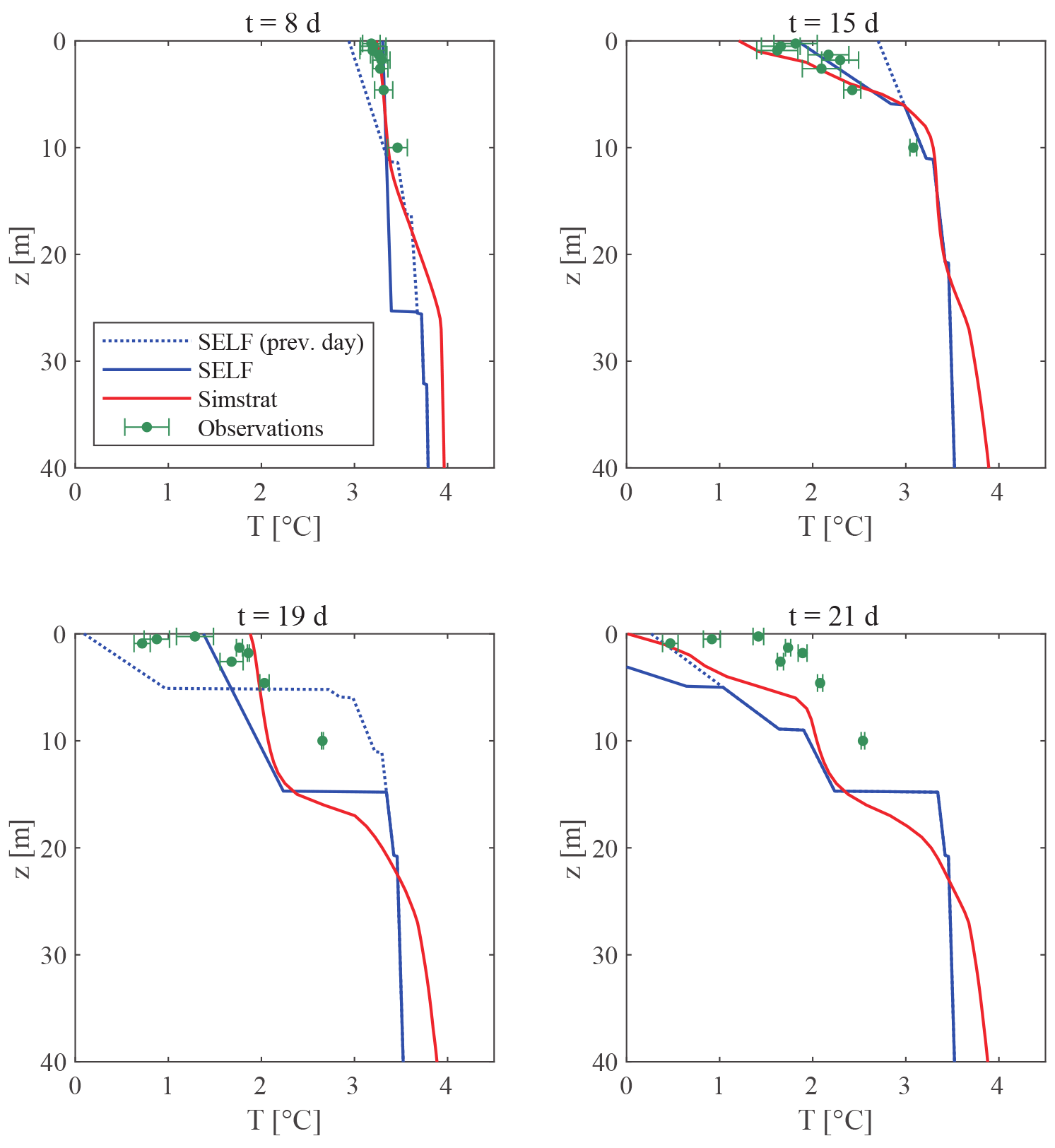
Figure 4Evolution of the temperature profile in the pre-freezing period for Lake Sils between 18 December 2016 and 8 January 2017. The plots represent the daily profiles obtained with SELF compared with the profiles at midnight computed by Simstrat. The dotted lines represent the SELF model's temperature profile on the previous day. The symbols represent the available observations, with the error band equal to 1 standard deviation of the temperature during the day.
The detailed analysis of the plots in Fig. 4 (where the profiles simulated with Simstrat are added for a comparison) allows us to understand how SELF works on these selected days. On day 8, a stronger wind thickens the surface layer when the stratification is weak: the change in SELF is discontinuous (as can be detected by comparing the solid line with the dotted line referring to the previous day), but the depth that is affected coincides with the end of the stratification in Simstrat. In calm conditions (day 15), the linear profile assumed by SELF in the surface mixed layer approximates the continuous Simstrat profile well. A strong wind event on day 19 produces a clear mixed layer of the same depth in the two models. Finally, the lake freezes on day 21 with an overall profile characterized by a similarly shaped profile.
For the selected year there are also in situ observations available: they are included in the different subplots of Fig. 4, making it possible to quantitatively evaluate the performance of the two models. There is an excellent agreement until day 18 (the whole sequence is provided in the Supplement). On day 18, both models responded to the increase in wind intensity by mixing the surface layer down to 15 m. This wind-mixing event is not observed in the in situ lake temperature data. Indeed, the temperature profile remains stratified during this period. The deviation from the observations of both models forced by the same atmospheric dataset shall not be interpreted as a deficiency of the models but rather as a need to provide more accurate on-lake meteorological data.
4.4 Performance of the minimal model
The duration of the pre-freezing period nd was estimated in three different ways. In all cases, the wind energy was externally prescribed, while differences exist in the computation of the heat loss, which depends on the LSWT, i.e., the result of the model itself. Thus, three options for the quantification of the heat loss were selected: (1) using the LSWT computed by Simstrat (case “Ts-Simstrat”) and thus an externally prescribed heat loss; (2) using the LSWT computed by SELF (case “Ts-SELF”), which uses the minimal model as a prognostic tool; and (3) using the LSWT from SELF as in the previous case but forcing the model with constant values of the meteorological variables averaged over the extended pre-freezing period (case “Ts-SELFav”).
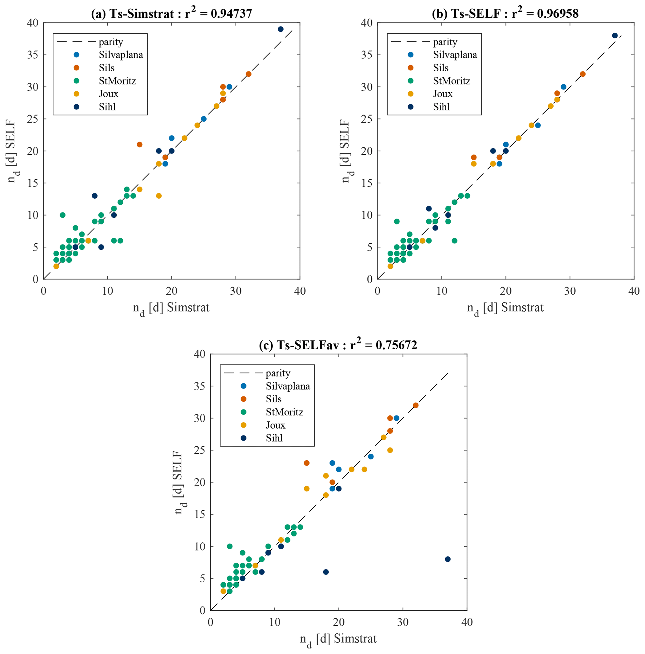
Figure 5Scatterplot of the duration of the pre-freezing period nd predicted by the minimal model (SELF) vs. the complete 1D model (Simstrat) using the net heat flux: (a) simulated by Simstrat, (b) reconstructed based on the LSWT estimated by SELF (prognostic mode, i.e., based only on purely meteorological data), and (c) reconstructed using averaged meteorological quantities (see Table 1).
The results are shown in Fig. 5, which reports the parity diagrams comparing Simstrat (assumed as the truth in this case) and SELF, with the three options for the computation of the heat loss. The overall agreement is very good for the “Ts-Simstrat” case (Fig. 5a, Pearson's r2=0.95) and even better for the “Ts-SELF” case (Fig. 5b, r2=0.97), with a decay of the performance, as expected, for the averaged “Ts-SELFav” case (Fig. 5c, r2=0.76). The SELF model provides realistic values of nd over a broad range of pre-freezing periods extending from 2 to almost 40 d for the five investigated lakes, a performance that is especially promising considering the simplicity of the minimal model. The improvement in the “Ts-SELF” case can be likely ascribed to the explicit consideration of the feedback that exists with LSWT in the determination of the heat fluxes from the lake to the atmosphere.
Table 2Calibrated parameters of the SELF model for the investigated lakes.

1 The efficiency η of energy transfer of Ew to ΔEp was calibrated for the five lakes in three different ways: using net heat fluxes directly from Simstrat, using LSWT from SELF to compute the fluxes (prognostic mode), and using seasonally averaged meteorological variables in the prognostic mode. 2 The coefficient k for the simplified analytical model (Eq. 10) was calibrated on the median value of the distribution of random sequences in SELF (further details in the Supplement).
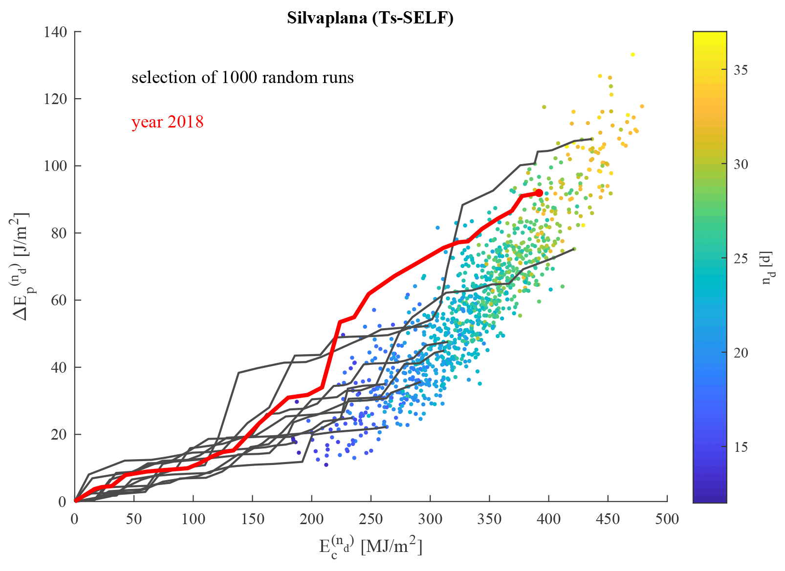
Figure 6Cumulative mixing energy vs. lost energy for Lake Silvaplana, as obtained from the random model. The color scale represents the duration of the pre-freezing period. Black trajectories correspond to random sequences; the red trajectory represents the pre-freezing period of a real winter (see Fig. 7).
The values of the wind-to-potential-energy efficiency η calibrated for the different lakes are variable (Table 2), with higher values for shallow lakes (Lakes Joux and Sihl) and lower values for the deepest lakes on the upper Engadine valley (Lakes Sils and Silvaplana). Lake St. Moritz, despite being of intermediate depth, is characterized by a value of η that is small, but it is also the lake with the smallest surface area, which reduces the wind fetch. However, we recall that η connects the wind energy to the lake mixing and thereby not only has a physical interpretation for the stratification process leading to ice formation but also serves as calibration parameter for the wind forcing. In this respect, wind speed is not measured from a lake buoy but at the lake shore or even farther in the case of Lake St. Moritz, where the nearby station is separated from the lake by a hill. The identification of the various factors affecting the efficiency η would require the analysis of a more extended database of lakes.
4.5 Monte Carlo analysis with SELF
The simplicity of the SELF model allows for the characterization of the pre-freezing period by exploring a large number of simulations following a Monte Carlo approach. We performed 100 000 runs with SELF (in the prognostic mode) for each lake, in which the time series of the wind energy and of the meteorological variables used to quantify the heat loss are randomly sorted from the actual sequences over the whole dataset of the extended pre-freezing period. The goal is to investigate the influence of the wind and of the cooling during the pre-freezing period and eventually to provide a simple analytical solution to predict the duration of the pre-freezing period.
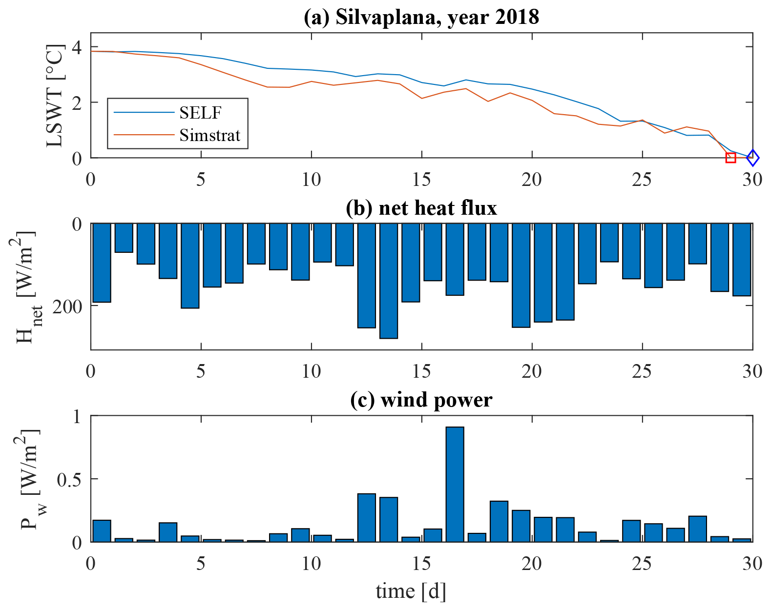
Figure 7Example of the dynamics in the pre-freezing period for winter 2018/19 in Lake Silvaplana corresponding to the red trajectory in Fig. 6: (a) comparison of the results of Simstrat and SELF (in the prognostic mode) with symbols representing the ice-on day, (b) daily averaged net heat flux (positive values for cooling), and (c) daily averaged wind power.
For each run, the freezing time nd is associated with the cumulated values of heat loss and mixing energy (depending on wind energy Ew through the efficiency η) and represented in a diagram using color-scaled dots (see Fig. 6 for Lake Silvaplana, where only 1000 random runs are plotted for clarity). This visualization illustrates that the length of the pre-freezing period is controlled by the amount of heat extracted but that it is also dependent on the input of the wind energy. Figure 6 also shows some examples of trajectories of the random runs (black lines) in the – plane and one sequence characterizing an actual winter (red line). The details of this single year are presented in Fig. 7, which shows the whole sequence of LSWT values simulated by Simstrat and SELF, respectively, together with the daily averaged net heat flux and wind power. The same analysis has been developed for the other lakes as well; please refer to the Supplement for the corresponding figures.
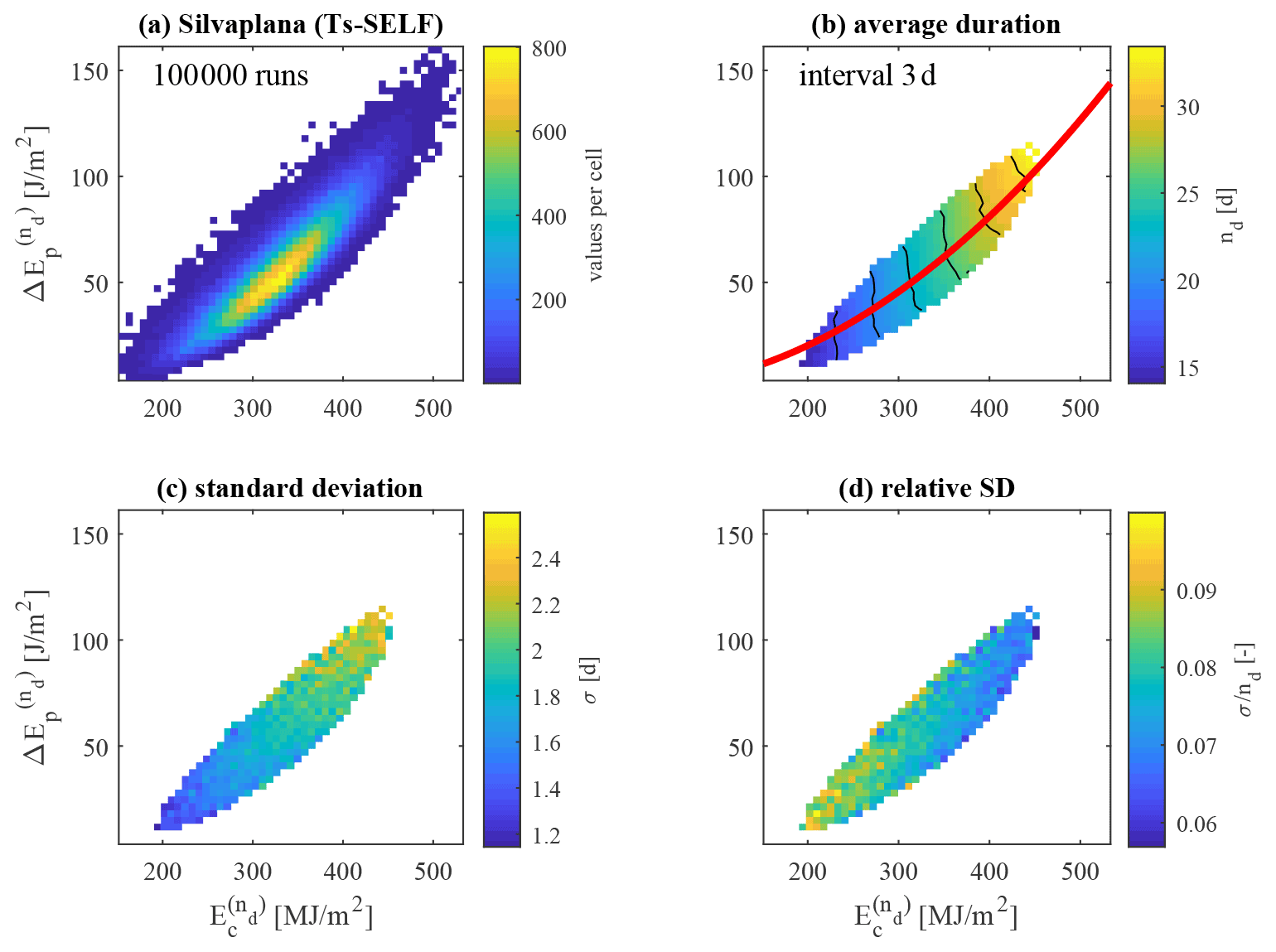
Figure 8Distribution of the results of the SELF model applied to 100 000 random sequences in Lake Silvaplana as a function of the cumulative values of the energies and : (a) number of results per computation cell; (b) average duration in days, nd, of the pre-freezing period, with black lines representing constant nd and the interval indicated in the plot; (c) standard deviation of nd in the cell; and (d) relative standard deviation. The thick red line in panel (b) represents the theoretical dependence obtained by means of the simplified analytical model (Eq. 10, using the coefficient k reported in Table 2).
Exploiting the total number of the Monte Carlo runs, it is possible to characterize the behavior of the process in a more exhaustive way. Figure 8 shows the results in the – plane, while Fig. 9 shows the results in the 〈ΔEp〉–〈Ec〉 plane, i.e., the mean daily energy fluxes. The two figures are built in the same way: Fig. 9a shows the distribution of all combinations; Fig. 9b reports the main result, i.e., the mean duration nd of the pre-freezing period; Fig. 9c shows the standard deviation of nd; and Fig. 9d shows the latter value normalized with the mean.
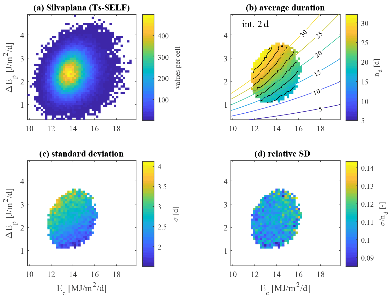
Figure 9The same results as in Fig. 8 but in terms of average daily values of the energies 〈ΔEp〉 and 〈Ec〉: (a) number of results per computation cell; (b) average duration in days, nd, of the pre-freezing period, with black curves representing constant nd with the interval indicated in the plot; (c) standard deviation of nd in the cell; and (d) relative standard deviation. The colored lines (colors associated with the color bar) in panel (b) represent the theoretical nd obtained by means of the simplified analytical model (Eq. 11; see also Fig. 8) with numbers indicating the estimated values of nd.
The analysis of the distribution of the points in the cloud in Fig. 6 suggests a relationship between and , with nd growing as the values of the two quantities increase. The duration nd grows from the lower-left corner to the upper-right corner of Fig. 8b, and the analytical curve from Eq. (10), shown with a red line, captures the general tendency of the minimal model's runs well. It is possible to identify an upper and a lower boundary, which represent, for a given wind history (which translates here into the cumulated mixing energy , hence along a horizontal line), the minimum and maximum cumulated loss of heat, respectively, under which ice can form. If more heat is extracted daily, the ice will form before, thus moving the point left and down; if less heat is extracted, ice will form later (point moving right and up) or not form at all if the process takes too long and the spring warming arrives. Figure 8d shows that the results are more variable in relative terms for the shorter pre-freezing period for which the actual history of the meteorological forcing matters even more.
The analysis of the results in the plane of the daily values (Fig. 9b) shows that the effect of the wind increases as it becomes faster and the cooling weaker (upper-left region), where the isolines with constant nd (represented by black lines) become more vertical. Hence, windy lakes will take longer to freeze, especially if they are not in a very cold climate. The general trend is predicted reasonably by the simplified analytical solution (colored lines with numbers representing nd values). The standard deviation shows higher values for windy and warm lakes (Fig. 9c) because of the stronger influence of the wind history with moderate variability in terms of its relative value (Fig. 9d). The figures for the other lakes are available in the Supplement.
5.1 Factors controlling the freezing time
The time series illustrated with a red trajectory in Fig. 6 shows that for a given energy loss (here ∼ 400MJ m−2) a change in mixing energy from ∼ 60 to 100 J m−2 will delay ice formation by about 5 d (see Fig. 8b) starting from the homothermal conditions. In order to have a reference to compare with, the observed trend in the ice-on date is 5.8 d per century in the Northern Hemisphere over the last 150 years (Magnuson, 2000); note that this delay is also affected by the shift of the day when homothermal conditions are realized. A variation of +67 % in the cumulated mixing energy (from ∼ 60 to ∼ 100 J m−2) corresponds to a change of mean wind speed of approximately +19 %, which is a relatively small change in the forcing given the cubic dependence. The timing also largely depends on the daily sequence of the wind power and heat exchanges (Fig. 7b and c), with single wind peaks producing much larger peaks in the mixing energy (and consequently on its cumulated value), again due to the cubic dependence.
Our results suggest that taking only the cooling into account (using for instance negative degree days, which depend solely on air temperature) may not explain the interannual variability in the ice formation and that the variability due to wind speed can be as large as the change resulting from a century of increase in air temperature. Adding the competition between cooling processes stratifying the water body and wind momentum destratifying the water body, as in SELF, allows for estimating the timing for ice formation more accurately.
SELF can be used to better understand long time series of ice formation in lakes (Magnuson, 2000) and specifically to decouple the interannual variability from the long-term climate-change-induced trend. A first effect of warming, which we do not discuss here, is the delay of the day when homothermal conditions occur. A second effect is the modification of the duration of the pre-freezing period. In this respect, the analysis based on random sequences suggests that the influence of wind increases for warm climates (low latitude and altitude) and that this effect might become relevant if wind change is sufficiently strong. If the interannual variability of ice phenology becomes larger than that of air temperature due to the effect of the wind, for instance, then ice phenology might become a confusing signal for climate change
In this study, we could not assess the role of lake depth in controlling the freezing process. This is an outcome from the investigated lakes, which are all deep, with maximum depths ranging from 22 to 77 m. However, water depth may become an important driver when the thickness of the surface mixed layer frequently encompasses the whole water depth.
5.2 Comparison and limitations of models to predict the freezing time
SELF is a minimal process-based model for predicting ice formation in lakes. Considering the stratification induced by cooling and the mixing induced by wind in an energy balance is a step forward compared to a more traditional accounting of air temperature through negative degree days (Franssen and Scherrer, 2008), statistical air temperature models (Livingstone and Adrian, 2009), or regression-tree-based prediction (Sharma et al., 2019). Those models have to assume that all the other parameters acting at the air–water interface, such as the wind action, stay constant over time. As a result, those approaches are not able to correctly predict the duration of the pre-freezing period: the correlation of nd with negative degree days, D, is generally poor for these lakes, with the exception of Lake Sils for which it is decent (see the details in the Supplement).
We have reported that the stochasticity in the wind speed and air temperature contributes to the timing of ice formation, and this element cannot be neglected in the majority of applications. Our energy-based model efficiently copes with this issue by comparing, on a daily timescale, the cooling-induced stratification and wind-induced mixing: the chronological sequence of these two factors has to be necessarily taken into account to correctly predict ice formation.
Describing the competition between stratification and destratification processes is typically the strength of 1D hydrodynamic models. However, SELF is computationally simple, and thousands of runs can be simulated in a few seconds, which is impossible with classical 1D hydrodynamic models. However, SELF has the same limitations as any 1D model: for instance, it does not consider the horizontal variability of ice formation, which typically starts from the shore and propagates offshore, introducing an uncertainty in the definition of a univocal ice-on date. In this respect, SELF was tested in five perialpine lakes of various sizes that sharing similar morphologies. The validity of SELF and more generally of any 1D model to very large systems remains to be demonstrated; another issue may arise from lakes with extended shallow areas. The deviation from the classical 1D framework of the heat budget as a function of morphology and latitude was recently shown for the end of the ice-covered period when lake dynamic is influenced by radiatively driven convection (Ulloa et al., 2019; Ramón et al., 2020). In the case of the pre-freezing period, the amount of heat stored in the sediment in the shallow area may affect the system (Fang and Stefan, 1996). However, the buffer role of the sediments in the heat budget was not investigated here. In this respect, large differences between SELF and observations of the pre-freezing duration can also be interpreted as interesting signatures of deviation from the classical 1D energy budget framework with other processes to be specifically investigated.
A further limitation of the model that might play a role in the proximity of homothermal conditions is not considering the effect of salinity on water density. While it is usually a second-order effect during summer stratification, when density is mostly dependent on water temperature, the existence of a vertical variability of the salinity may become relatively more important when the temperature is approximately uniform, with consequences on the freezing time in saline lakes (Stepanenko et al., 2019). Adding this factor in the minimal model is possible but would require the inclusion of a sub-model for the salinity profile and additional data that are not routinely available.
Finally, we note that the model requires the estimate of a single parameter, the global efficiency η. Obtaining an accurate value of this parameter based on theoretical considerations is a difficult task (see the discussion in the Supplement for some hints) and would require a much deeper hydro-dynamic and aerodynamic analysis. However, it is clear that the calibration of one parameter is not particularly challenging and can be pursued even if the available data are relatively limited. It is also important to recognize that the time step Δt plays a role both in the definition of the well-mixed layer thickness (through Ew) and in the quantification of the heat loss Ec; the choice of a daily time step is the most appropriate choice because it integrates the main periodicity of the external forcing.
5.3 Implications
The minimal model was designed to provide a simple process-based tool to estimate freezing dates in lakes. SELF can be easily generalized at global scale as an operational prognostic product, as it relies on easily accessible quantities: surface heat fluxes (which can be computed using variables from nearby meteorological stations or from global meteorological models, for instance) and dates for homothermal lake temperature. The necessary occurrence of homothermal conditions at the temperature of maximum density (4 ∘C), which can be detected from remotely sensed LSWT, can provide accurate initial conditions to model the energy competition with SELF.
A follow-up study should aim to use global meteorological data and remotely sensed temperature measurements from satellites to predict the timing of ice formation and potentially contribute to the monitoring of this essential climate variable, as defined by GCOS (https://gcos.wmo.int/en/essential-climate-variables/lakes/, last access: 26 April 2021). Note that the only tuning parameter from SELF can be calibrated for each lake based on satellite-based observations of nd. As mentioned above, the homothermal conditions can be probed with a satellite (infrared) optical radiometer, and ice formation can be operationally tracked with either optical or microwave remote sensing techniques (Duguay et al., 2014). Finally, there is a practical interest in SELF for lake managers as the model can be used to provide a short-term probability of the timing for ice formation. This kind of information may help stakeholders effectively face the strong interannual variability in ice phenology.
We developed a minimal model, SELF, to predict the duration of the pre-freezing period ranging from the early winter lake's overturn to the formation of an ice sheet at the surface. We showed that the temporal evolution of the thermal structure during this period is governed by the competition between cooling of the surface water due to the heat lost to the atmosphere and mixing of the surface layer due to wind. We demonstrated that including only those two physical processes in SELF is sufficient to describe the first-order dynamics of the inverse stratification process with only one calibration parameter. An approximate analytical solution obtained by further simplifying the minimal model in the ideal case of constant mechanical and thermal energy input can be used to sketch the general tendency of the system, highlighting the approximate power law dependence on the energy fluxes and eventually replacing traditional integral approaches such as negative degree days.
The simplicity of the model allowed us to perform Monte Carlo simulations and characterize the process as a function of the cumulated or daily averaged values of the energy fluxes in statistical terms. Such analysis showed that the history of the system (i.e., the actual sequence of the atmospheric forcing) is crucial to determine the duration of the pre-freezing period exactly, but a general tendency can be recognized. We suggest that this competition between wind and heat loss could partly explain the strong interannual variability observed in the ice-on phenology worldwide.
In this work, we have focused on the mechanistic definition of the minimal model SELF with a validation restricted to alpine lakes. Now we encourage two immediate applications of SELF. First, this model can be used on a global scale to help understanding change in ice phenology. Second, the model could be used to help stakeholders evaluate the short-term probability of ice formation on their lakes.
The source code of SELF (https://doi.org/10.5281/zenodo.5082374, Toffolon et al., 2021) is available at https://github.com/marcotoffolon/SELF (last access: 8 July 2021).
Lake observations are available from the following sources: https://doi.org/10.25678/0000PP (Bouffard, 2019b), https://doi.org/10.25678/0000KK (Bouffard, 2019c), https://doi.org/10.25678/0000MM (Bouffard, 2019a), and https://doi.org/10.25678/0000QQ (Bouffard, 2016).
The supplement related to this article is available online at: https://doi.org/10.5194/gmd-14-7527-2021-supplement.
DB and MT designed the research. MT, DB, and LC conducted the research. MT, DB, and LC wrote the manuscript.
The contact author has declared that neither they nor their co-authors have any competing interests.
Publisher's note: Copernicus Publications remains neutral with regard to jurisdictional claims in published maps and institutional affiliations.
The authors would like to thank Nathalie Dubois (Eawag) for collecting and providing lake temperature data from Lac de Joux; Jean-Daniel Meylan (fisherman) for his long-term record of ice phenology at Lac de Joux; and Michael Plüss (Eawag) and Felix Keller (Academia Engiadina) for the lake temperature and ice measurements in Engadine's lake. Hugo Ulloa is thanked for discussions relating to the paper. Damien Bouffard acknowledges support from GCOS Switzerland and Academia Engiadina.
This research has been partly supported by MeteoSwiss in the framework of GCOS Switzerland and Academia Engiadina.
This paper was edited by Andrew Wickert and reviewed by two anonymous referees.
Bilello, M. A.: Method for predicting river and lake ice formation, J. Appl. Meteorol. Clim., 3, 38–44, 1964. a
Bouffard, D.: Silvaplanersee_T-Mooring, Eawag: Swiss Federal Institute of Aquatic Science and Technology [data set], https://doi.org/10.25678/0000QQ, 2016. a
Bouffard, D.: Sihlsee_T-Mooring, Eawag: Swiss Federal Institute of Aquatic Science and Technology [data set], https://doi.org/10.25678/0000MM, 2019a. a
Bouffard, D.: Silsersee_T-Mooring, Eawag: Swiss Federal Institute of Aquatic Science and Technology [data set], https://doi.org/10.25678/0000PP, 2019b. a
Bouffard, D.: St.Moritzersee_T-Mooring, Eawag: Swiss Federal Institute of Aquatic Science and Technology [data set], https://doi.org/10.25678/0000KK, 2019c. a
Dibike, Y., Prowse, T., Saloranta, T., and Ahmed, R.: Response of Northern Hemisphere lake-ice cover and lake-water thermal structure patterns to a changing climate, Hydrol. Process., 25, 2942–2953, https://doi.org/10.1002/hyp.8068, 2011. a
Duguay, C. R., Flato, G. M., Jeffries, M. O., Ménard, P., Morris, K., and Rouse, W. R.: Ice-cover variability on shallow lakes at high latitudes: model simulations and observations, Hydrol. Process., 17, 3465–3483, https://doi.org/10.1002/hyp.1394, 2003. a
Duguay, C. R., Bernier, M., Gauthier, Y., and Kouraev, A.: Remote sensing of lake and river ice, in: Remote Sensing of the Cryosphere, edited by: Tedesco, M., John Wiley & Sons, Ltd, Hoboken, NJ, USA, 273–306, 2014. a
Fang, X. and Stefan, H. G.: Dynamics of heat exchange between sediment and water in a lake, Water Resour. Res., 32, 1719–1727, https://doi.org/10.1029/96WR00274, 1996. a
Franssen, H. J. H. and Scherrer, S. C.: Freezing of lakes on the Swiss plateau in the period 1901–2006, Int. J. Climatol., 28, 421–433, https://doi.org/10.1002/joc.1553, 2008. a, b, c
Gaudard, A., Råman Vinnå, L., Bärenbold, F., Schmid, M., and Bouffard, D.: Toward an open access to high-frequency lake modeling and statistics data for scientists and practitioners – the case of Swiss lakes using Simstrat v2.1, Geosci. Model Dev., 12, 3955–3974, https://doi.org/10.5194/gmd-12-3955-2019, 2019. a, b, c, d
Goudsmit, G.-H., Burchard, H., Peeters, F., and Wüest, A.: Application of k-ϵ turbulence models to enclosed basins: The role of internal seiches, J. Geophys. Res., 107, 3230, https://doi.org/10.1029/2001JC000954, 2002. a, b, c
Hipsey, M. R., Bruce, L. C., Boon, C., Busch, B., Carey, C. C., Hamilton, D. P., Hanson, P. C., Read, J. S., de Sousa, E., Weber, M., and Winslow, L. A.: A General Lake Model (GLM 3.0) for linking with high-frequency sensor data from the Global Lake Ecological Observatory Network (GLEON), Geosci. Model Dev., 12, 473–523, https://doi.org/10.5194/gmd-12-473-2019, 2019. a
Kullenberg, G. E. B.: On vertical mixing and the energy transfer from the wind to the water, Tellus, 28, 159–165, 1976. a
Leppäranta, M.: A review of analytical models of sea‐ice growth, Atmos. Ocean, 31, 123–138, https://doi.org/10.1080/07055900.1993.9649465, 1993. a
Leppäranta, M.: Interpretation of statistics of lake ice time series for climate variability, Hydrol. Res., 45, 673–683, https://doi.org/10.2166/nh.2013.246, 2014. a
Leppäranta, M.: Freezing of Lakes and the Evolution of their Ice Cover, Springer, Berlin Heidelberg, 2015. a, b
Liston, G. E. and Hall, D. K.: An energy-balance model of lake-ice evolution, J. Glaciol., 41, 373–382, 1995. a
Livingstone, D. M.: An example of the simultaneous occurrence of climate-driven “sawtooth” deep-water warming/cooling episodes in several Swiss lakes, Internationale Vereinigung für theoretische und angewandte Limnologie: Verhandlungen, 26, 822–828, 1997. a
Livingstone, D. M. and Adrian, R.: Modeling the duration of intermittent ice cover on a lake for climate-change studies, Limnol. Oceanogr., 54, 1709–1722, https://doi.org/10.4319/lo.2009.54.5.1709, 2009. a
Livingstone, D. M., Adrian, R., Blenckner, T., George, G., and Weyhenmeyer, G. A.: Lake Ice Phenology, in: The Impact of Climate Change on European Lakes, edited by: George, G., Springer, Dordrecht, Netherlands, 51–61, https://doi.org/10.1007/978-90-481-2945-4_4, 2010. a
MacKay, M. D., Verseghy, D. L., Fortin, V., and Rennie, M. D.: Wintertime Simulations of a Boreal Lake with the Canadian Small Lake Model, J. Hydrometeorol., 18, 2143–2160, https://doi.org/10.1175/JHM-D-16-0268.1, 2017. a
Magnuson, J. J.: Historical Trends in Lake and River Ice Cover in the Northern Hemisphere, Science, 289, 1743–1746, https://doi.org/10.1126/science.289.5485.1743, 2000. a, b, c, d
Martin, J. L. and McCutcheon, S. C.: Hydrodynamics and Transport for Water Quality Modeling, Lewis Publications, New York, 1999. a
Ramón, C. L., Ulloa, H. N., Doda, T., Winters, K. B., and Bouffard, D.: Bathymetry and latitude modify lake warming under ice, Hydrol. Earth Syst. Sci., 25, 1813–1825, https://doi.org/10.5194/hess-25-1813-2021, 2021. a
Read, J. S., Hamilton, D. P., Jones, I. D., Muraoka, K., Winslow, L. A., Kroiss, R., Wu, C. H., and Gaiser, E.: Derivation of lake mixing and stratification indices from high-resolution lake buoy data, Environ. Modell. Softw., 26, 1325–1336, 2011. a
Rodhe, B.: On the relation between air temperature and ice formation in the Baltic, Geogr. Ann., 34, 175–202, 1952. a
Sharma, S., Blagrave, K., Magnuson, J. J., O’Reilly, C. M., Oliver, S., Batt, R. D., Magee, M. R., Straile, D., Weyhenmeyer, G. A., Winslow, L., and Woolway, R. I.: Widespread loss of lake ice around the Northern Hemisphere in a warming world, Nat. Clim. Change, 9, 227–231, https://doi.org/10.1038/s41558-018-0393-5, 2019. a
Stepanenko, V., Repina, I. A., Ganbat, G., and Davaa, G.: Numerical Simulation of Ice Cover of Saline Lakes, Izv. Atmos. Ocean. Phy.+, 55, 129–138, https://doi.org/10.1134/S0001433819010092, 2019. a
Toffolon, M., Cortese, L., and Bouffard, D.: SELF, v1.0, Zenodo [code], https://doi.org/10.5281/zenodo.5082374, 2021 (data available at: https://github.com/marcotoffolon/SELF, last access: 8 July 2021). a
Ulloa, H. N., Winters, K. B., Wüest, A., and Bouffard, D.: Differential Heating Drives Downslope Flows that Accelerate Mixed-Layer Warming in Ice-Covered Waters, Geophys. Res. Lett., 46, 13872–13882, https://doi.org/10.1029/2019GL085258, 2019. a
Weyhenmeyer, G. A., Livingstone, D. M., Meili, M., Jensen, O., Benson, B., and Magnuson, J. J.: Large geographical differences in the sensitivity of ice-covered lakes and rivers in the Northern Hemisphere to temperature changes, Glob. Change Biol., 17, 268–275, https://doi.org/10.1111/j.1365-2486.2010.02249.x, 2011. a
Wüest, A. and Lorke, A.: Small-scale hydrodynamics in lakes, Annu. Rev. Fluid Mech., 35, 373–412, https://doi.org/10.1146/annurev.fluid.35.101101.161220, 2003. a