Robustness of neural network emulations of radiative transfer parameterizations in a state-of-the-art general circulation model

The ability of machine-learning-based (ML-based) model components to generalize to the previously unseen inputs and its impact on the stability of the models that use these components have been receiving a lot of recent attention, especially in the context of ML-based parameterizations. At the same time, ML-based emulators of existing physically based parameterizations can be stable, accurate, and fast when used in the model they were specifically designed for. In this work we show that shallow-neural-network-based emulators of radiative transfer parameterizations developed almost a decade ago for a state-of-the-art general circulation model (GCM) are robust with respect to the substantial structural and parametric change in the host model: when used in two 7-month-long experiments with a new GCM, they remain stable and generate realistic output. We concentrate on the stability aspect of the emulators' performance and discuss features of neural network architecture and training set design potentially contributing to the robustness of ML-based model components.

1 Introduction

One of the main difficulties in developing and implementing high-resolution environmental models is the complexity of the physical processes involved. For example, the calculation of radiative transfer in a general circulation model (GCM) often takes a significant part of the total model run time. From the standpoint of basic physics, radiative transfer is well understood. Very accurate but computationally complex benchmark models exist (Oreopoulos et al., 2012) that demonstrate excellent agreement with observations (Turner et al., 2004). Parameterizations of radiative transfer seek a compromise between accuracy and computational performance. Arguably, the biggest simplification they make is treatment of radiative transfer as a 1-D as opposed to a 3-D process (independent column approximation, ICA): both solar, or shortwave (SW )radiation, and terrestrial, or longwave (LW) radiation, are considered to flow within the local column of the model, up and down the local vertical (two-stream approximation) but not between columns. This approximation works well at spatial resolutions characteristic of general circulation models of the atmosphere (Marshak and Davis, 2005). To integrate over the spectrum of radiation, parameterizations split it into several broad bands and a number of representative spectral intervals that are treated monochromatically (Fu and Liou, 1992). State-of-the-art parameterizations can reproduce benchmark calculations to a high degree of accuracy even with these simplifications, but they still require substantial computational expense.

Radiative transfer parameterizations supply their host model with broadband fluxes and heating rates, which are obtained by integration over time, space, and frequency. Therefore, a trade-off between accuracy and computational expense can be found in how finely these dimensions are discretized (Hogan et al., 2017).

• Discretization in time – all GCMs update their radiative heating and cooling rates less frequently than the rest of the model fields. For example, the National Centers for Environmental Prediction (NCEP) Global Forecast System (GFS) v16 general circulation model (GCM) in its operational configuration updates its radiative fields once per model hour, while updates to temperature, moisture, and most cloud properties due to unresolved physics processes happen every 150 model seconds or 24 times per single radiation call. Updates due to dynamical processes happen even more frequently: every 12.5 s (Kain et al., 2020). This approximation is good for slowly changing fields of certain radiatively active gases but is less justified for small-scale clouds with lifetimes of an hour or less.

• Discretization in space – some GCMs calculate radiative fields on a coarser spatial grid and interpolate them onto a finer grid used for the rest of the model variables. For example, the radiation grid in the European Centre for Medium-Range Weather Forecasts (ECMWF) Integrated Forecast System (IFS) v43R3 in the ensemble mode is 6.25 times coarser than the physics grid (Hogan et al., 2017). This may cause 2 m temperature errors in areas of surface heterogeneity, e.g., coasts (Hogan and Bozzo, 2015).

• Discretization and sampling in frequency space – the Rapid Radiative Transfer Model (RRTMG), a parameterization of radiative transfer for GCMs used in NCEP GFS and ECMWF IFS, utilizes 14 bands in the shortwave (Mlawer et al., 1997), while the parameterization used in the United Kingdom Met Office Unified Model utilizes 6 (Edwards and Slingo, 1996). Monte Carlo spectral integration (Pincus and Stevens, 2009) performs integration over only a part of the radiative spectrum randomly chosen at each point in time and space, allowing us to increase the temporal and spatial resolution of radiation calculations. Monte Carlo integration of the independent column approximation (McICA) (Pincus et al., 2003) integrates over the entire spectrum but samples subgrid-scale (SGS) cloud properties in a random, unbiased manner in each grid column in time and space instead of integrating over them.

All of the methods for improving computational efficiency of radiative transfer parameterizations outlined above are either numerical and/or statistical in nature. In recent years there has been a substantial increase in interest in adding machine learning (ML) techniques to the arsenal of these methods (Boukabara et al., 2019). It has been accomplished in at least two different ways: (1) as an emulation technique for accelerating calculations of radiative transfer parameterizations or their components and (2) as a tool for the development of new parameterizations based on data simulated by more sophisticated models and/or reanalysis.

An ML-based emulator of a model physics parameterization is a functional imitation of this parameterization in the sense that the results of model calculations with the original parameterization and with its ML emulator are so close to each other by a metric appropriate for an application at hand as to be identical for the practical purposes. From the mathematical point of view, model physics and individual parameterizations are mappings,

$$\begin{array}{}\text{(1)}& \mathit{Y}=M\left(X\right);\mathit{X}\in {\mathrm{\Re }}^n,\mathrm{and},\mathit{Y}\in {\mathrm{\Re }}^m,\end{array}$$

where n and m are the dimensionalities of the input and output vector spaces, respectively. Therefore, emulating existing parameterizations using ML techniques is a mapping approximation problem. In practice, this mapping can be defined by a set of its input and output vectors that is obtained by running the original model with the parameterization that is to be emulated and saving inputs and outputs of this parameterization with a frequency and spatiotemporal coverage sufficient to comprehensively cover the domain and range of the mapping. These data are then used for the emulator training. This approach allows us to achieve a very high accuracy of approximation because model output, unlike empirical data, is neither noisy nor sparse.

The domain and range of the mapping are defined not only by the parameterization that is being emulated but by the entirety of the atmospheric model environment: the dynamical core, the suite of physical parameterizations, and the set of configuration parameters for both. Once any of these components and/or parameters are modified, the set of possible model states is altered as well, possibly now including states that were absent in the emulator's training data set.

How accurately should the emulator approximate the original mapping? Unbiased, random, uncorrelated errors in radiative heating rates with magnitudes as large as the net cooling rate do not statistically affect the forecast skill of an atmospheric model (Pincus et al., 2003). From the physical standpoint this can be understood in the following way: random small local heating rate errors in the bulk of the atmosphere lead to local small-scale instabilities that are mixed away by the flow; however, there is no such mechanism for the surface variables, such as skin temperature, and errors in surface fluxes can be more consequential (Pincus and Stevens, 2013). Therefore, it may be useful to think of the above as necessary conditions on an approximation error of an ML emulator of a radiative transfer parameterization for it to be a successful functional imitation of the original scheme.

Developing a stable and robust neural-network-based (NN-based) emulator is a multifaceted problem that requires deep understanding of multiple technical aspects of the training process and details of NN architecture. Many techniques for the stabilization of hybrid statistical–deterministic models have been developed. Compound parameterization has been proposed for climate and weather modeling applications for which an additional NN is trained to predict errors of the NN emulator, and, if the predicted error is above a certain threshold, compound parameterization falls back to calling the original physically based scheme (Krasnopolsky et al., 2008b). Stability theory was used to identify the causes and conditions for instabilities in ML parameterizations of moist convection when coupled to an idealized linear model of atmospheric dynamics (Brenowitz et al., 2020). An NN optimization via random search over hyperparameter space resulted in considerable improvements in the stability of subgrid physics emulators in the super-parameterized Community Atmospheric Model version 3.0 (Ott et al., 2020). A coupled online learning approach was proposed whereby a high-resolution simulation is nudged to the output of a parallel lower-resolution hybrid model run and the ML component of the latter is retrained to emulate tendencies of the former, helping to eliminate biases and unstable feedback loops (Rasp, 2020). The random forest approach was successfully used to build a stable ML parameterization of convection (Yuval and O'Gorman, 2020). Physical constraints were used to achieve the stability of hybrid models (e.g., Yuval et al., 2021; Kashinath et al., 2021).

In this work we present robust and stable shallow-NN-based emulators of radiative transfer parameterizations. We explore how much of a change in the model's phase space (as well as the original parameterization's domain and range) a statistical model like the NN can tolerate. We will approach this question by installing shallow-NN-based emulators of LW and SW RRTMG developed in 2011 for the NCEP Climate Forecast System (CFS) (Krasnopolsky et al., 2010) into the new version 16 of NCEP GFS that became operational in March of 2021. Given the scope of changes in the host model (described in Sect. 3), we do not expect results of parallel runs to be identical; therefore, we will mostly concentrate on the stability aspect of the emulators' performance.

In Sect. 2, we briefly describe design aspects of these and other emulators of radiative transfer parameterizations reported in the literature so far. In Sect. 3, we outline major differences between the 2011 version of CFS and the GFS v16, and we describe numerical experiments with SW and LW emulators developed for the 2011 version of CFS (Krasnopolsky et al., 2010) and incorporated into GFS v16. Results of these experiments are examined in Sect. 4. Section 5 discusses aspects of neural network architecture and training set design potentially contributing to the stability of ML-based model components. Conclusions are formulated in Sect. 6.

2 Survey on technical aspects of existing ML emulators of radiative transfer parameterizations

NeuroFlux, a shallow-neural-network-based LW radiative transfer parameterization developed at ECMWF, was in part an emulator and in part a new ML-based parameterization (Chevallier et al., 1998, 2000). It consisted of multiple NNs, each utilizing a hyperbolic tangent as an activation function (AF) but using a varying number of neurons in the single hidden layer: two NNs were used to generate vertical profiles of upwelling and downwelling clear-sky LW fluxes per each vertical layer, and a battery of NNs, two per each vertical layer of the host model, was used to compute profiles of upwelling and downwelling fluxes due to black-body cloud on a given layer, with overall fluxes calculated using the multilayer gray-body model. The training set for clear-sky NNs contained 6000 cloudless profiles from global ECMWF short-range forecasts; 1 d of 3-hourly data per month of a single year were utilized. From this set, multiple training sets for cloudy-sky NNs were derived, each containing 6000 profiles as well: a cloud with the emissivity of unity was artificially introduced on a given vertical layer, and radiative transfer parametrization was used in the offline mode to calculate resulting radiative fields. NeuroFlux was accurate and about 1 order of magnitude as fast as the original parameterization in a model with 31 vertical layers. It was used operationally within the ECMWF four-dimensional variational data assimilation system (Janiskova et al., 2002). However, in model configurations with 60 vertical layers and above, NeuroFlux could not maintain the balance between speed-up and accuracy (Morcrette et al., 2008).

The approach based on pure emulation of existing LW and SW radiative transfer parameterizations using NNs has been pursued at the NCEP Environmental Modeling Center (Krasnopolsky et al., 2008a, 2010, 2012; Belochitski et al., 2011). In this approach, two shallow NNs with hyperbolic tangent activation functions, one for LW and the other for SW radiative transfer, generate heating rate profiles as well as surface and top-of-the-atmosphere radiative fluxes, replacing the entirety of respective RRTMG LW and SW parameterizations. It was not only radiative transfer solvers that were emulated but also the calculations of gas and cloud optical properties (aerosol optical properties were prescribed from climatology). Two different pairs of emulators were designed for two different applications: climate simulation and medium-range weather forecast, each differing in the training set design. The database for the former application was generated by running the NCEP CFS, a state-of-the-art fully coupled climate model, for 17 years (1990–2006) and saving instantaneous inputs and outputs of RRTMG every 3 h for 1 d on the 1st and the 15th of each month to sample diurnal and annual cycles, as well as decadal variability and states introduced by time-varying greenhouse gases and aerosols. From this database, 300 global snapshots were randomly chosen and consequently split into three independent sets for training, testing, and validation, each containing about 200 000 input/output records (Krasnopolsky et al., 2010). The data set for the medium-range forecast application was obtained from a total of 24 10 d NCEP GFS forecasts initialized on the 1st and the 15th of each month of 2010, with each forecast saving instantaneous 3-hourly data. Independent data sets were obtained following the same procedure as for the climate application (Krasnopolsky et al., 2012).

The dimensionality of data sets and NN input vectors for both applications was reduced in the following manner: some input profiles (e.g., pressure) that are highly correlated in the vertical were sampled on every other level without a decrease in approximation accuracy; some inputs that are uniformly constant above a certain level (water vapor) or below a certain level (ozone) were excluded from the training set on these levels; inputs that are given by prescribed monthly climatological lookup tables (e.g., trace gases, tropospheric aerosols) were replaced by latitude and periodic functions of longitude and month number; inputs given by prescribed monthly time series (e.g., carbon dioxide, stratospheric aerosols) were replaced by the year number and periodic function of month number. No reduction in dimensionality was applied to outputs.

A very high accuracy and up to 2 orders of magnitude increase in speed compared to the original parameterization for both NCEP CFS and GFS full radiation have been achieved for model configurations with 64 vertical levels. The systematic errors introduced by NN emulations of full model radiation were negligible and did not accumulate during the decadal model simulation. The random errors of NN emulations were also small. Almost identical results have been obtained for the parallel multi-decadal climate runs of the models using the NN and the original parameterization as well as in the limited testing in the medium-range forecasting mode. Regression trees were explored as an alternative to NNs and were found to be nearly as accurate in a 10-year-long climate run while requiring much more computer memory due to the fact that the entire training data set has to be stored in memory during model integration (Belochitski et al., 2011).

Using the approach developed at NCEP, an emulator of RRTMG consisting of a single shallow NN that replaces both LW and SW parameterizations at once was developed at the Korean Meteorological Agency for the short-range weather forecast model Korea Local Analysis and Prediction System in an idealized configuration with 39 vertical layers (Roh and Song, 2020). Inputs and outputs to RRTMG were saved on each 3 s time step of a 6 h long simulation of a squall line, and about 270 000 input/output pairs were randomly chosen from this data set to create training, validation, and testing sets. Dimensionality reduction was performed by removing constant inputs. Several activation functions were tested (tanh, sigmoid, softsign, arctan, linear), with hyperbolic tangent providing the best overall accuracy of approximation. The emulator was 2 orders of magnitude as fast as the original parameterization and was stable in a 6 h long simulation.

Two dense, fully connected, feed-forward deep-NN-based emulators with three hidden layers, one emulator per parametrization, were developed for the LW and SW components of RRTMG Parallel (RRTMG-P) (Pincus et al., 2019) for the Department of Energy's super-parameterized Energy Exascale Earth System Model (SP-E3SM) (Pal et al., 2019). In SP-E3SM, radiative transfer parameterizations act in individual columns of a 2-D cloud-resolving model with 31 vertical levels embedded into columns of the host GCM. The calculation of cloud and aerosol optical properties was not emulated; instead, original RRTMG-P subroutines were used. Inputs and outputs of radiative parameterizations were saved at every time step of a year-long model run, with 9 % of these data randomly chosen to form a data set of 12 000 000 input/output records for the LW and of 6 000 000 input/output records for the SW emulator training and validation. In total, 90 % of the data in these sets was used for training and 10 % for validation and testing. No additional dimensionality reduction was performed. Sigmoid AF was chosen as it was found to provide slightly better training convergence than the hyperbolic tangent. The emulator was 1 order of magnitude faster than the original parametrization and was stable in a year-long run.

A number of ML-based radiative transfer parameterizations or their components have been developed but, to our knowledge, have not yet been tested in an online setting or in interactive coupling to an atmospheric model. Among them are deep-NN-based parameterizations of gas optical properties for RRTMG-P (Ukkonen et al., 2020; Veerman et al., 2021) and a SW radiative transfer parameterization based on convolutional deep neural networks (Lagerquist et al., 2021).

3 Design of numerical experiments with GFS v16

GFS v16 differs from the 2011 version of the atmospheric component of NCEP CFS in a number of ways, the most relevant of which are summarized in Table 1.

Table 1 Differences between the atmospheric component of 2011 NCEP CFS and the 2021 version of NCEP GFS.

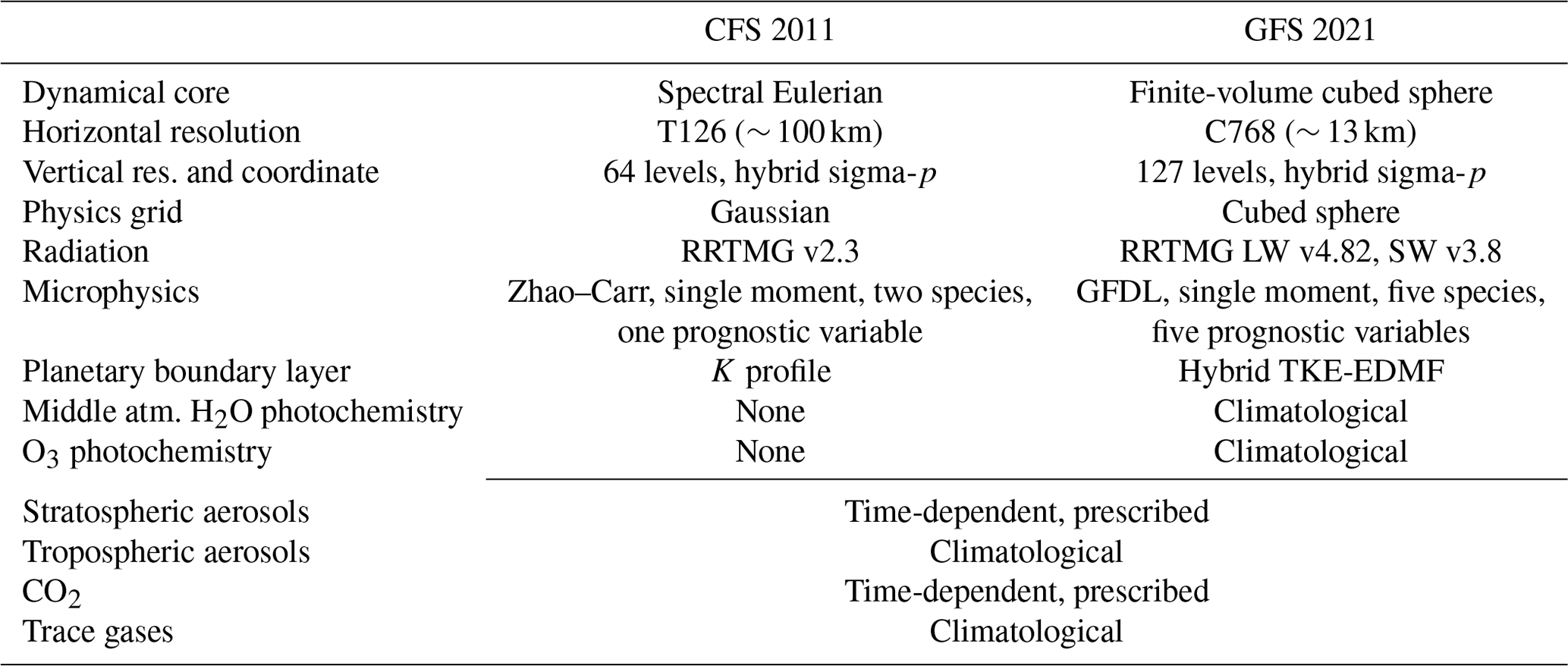
From the standpoint of the implementation of radiative transfer emulators developed in 2011 into the modern generation of GFS, the most consequential change in the model is the near doubling of the number of vertical layers because it has a direct impact on the size of the input layer of the NN-based emulator. Therefore, we reconfigure GFS v16 to run with 64 layers in the vertical.

Another consequential change in the model appears to be the replacement of the Zhao–Carr microphysics (Zhao and Carr, 1997) with the GFDL scheme (Lin et al., 1983; Chen and Lin, 2011; Zhou et al., 2019). Using the latter in combination with 2011 RRTMG emulators resulted in unphysical values of outgoing LW radiation at the top of the atmosphere (TOA) (not shown). A potential explanation is that the change in microphysical parameterization leads to an increase in the number of the model's prognostic variables. Both the spectral and the finite-volume dynamical cores include zonal and meridional wind components, pressure, temperature, water vapor, and ozone mixing ratios as prognostic variables. The Zhao–Carr microphysics add only one more prognostic to this list: the mixing ratio of total cloud condensate (defined as the sum of cloud water and cloud ice mixing ratios). The GFDL microphysics add six prognostic variables: cloud water, cloud ice, rain, snow, and graupel mixing ratios, as well as cloud fraction. The near doubling of the number of prognostic variables from 7 to 12 leads to the proportional increase in the dimensionality of the physical phase space of the model. As a result, the set of possible model states in GFS v16 is very different, from a mathematical standpoint, than in the 2011 CFS. Even though the vector of inputs to the LW parameterization remains the same in the new model, it is obtained by mapping from a very different mathematical object, potentially increasing the probability that a given input vector lies outside the NN's original training data set domain. For our experiments, we replaced the GFDL microphysical parametrization with the Zhao–Carr scheme.

The new hybrid TKE-EDMF planetary boundary layer (PBL) parameterization (Han and Bretherton, 2019) also introduces a new prognostic variable, subgrid-scale turbulent kinetic energy, that was absent in the 2011 version of CFS. Even though we did not see adverse effects stemming from the use of the new PBL scheme in preliminary testing, we replaced it with the original K profile and/or EDMF scheme (Han and Pan, 2011) out of caution.

Concentrations of radiatively active gases are important inputs to radiative transfer schemes and, more generally, are important parameters of the Earth system. From the standpoint of emulator training, a change in these parameters leads to a change in phase space of the host model, potentially necessitating retraining of the emulator to ensure its accuracy and stability. CO₂ concentration values used during training of 2011 emulators ranged from 350 to 380 ppmv between the years 1990 and 2006, respectively. In our current experiments spanning 2018, the CO₂ concentration was about 409 ppmv, or about 10 % higher on average than in the training set.

There were incremental updates and parametric changes to all other components of the suite of physical parameterizations, which are too numerous to be listed here; in addition, the model's software infrastructure was completely overhauled, including a new modeling framework based on the Earth System Modeling Framework (ESMF), a coupler of the dynamical core to the physics package, an input/output system, and workflow scripts (for more detail, see the document “GFS/GDAS Changes Since 1991” at https://www.emc.ncep.noaa.gov/gmb/STATS/html/model_changes.html, last access: 27 November 2021.).

For experiments presented in this paper, we configure GFS v16 to run at C96 horizontal resolution (∼ 100 km) to reduce the computational expense of the model. This configuration will be referred to as GFS in the following discussion and was used in control runs. We then replaced both modern versions of LW and SW RRTMG parameterizations in GFS with radiative transfer emulators developed in Krasnopolsky et al. (2010). This version of the model will be referred to as hybrid deterministic–statistical GFS, or HGFS. Two 7-month-long runs were performed with each model configuration: one initialized on 1 January 2018 and the other one on 1 July 2018, both using 2018 values of radiative forcings, with the instantaneous output saved 3-hourly. Sea surface temperatures (SSTs) in GFS forecasts are initialized from analysis and exponentially relax to climatology on a 90 d timescale as forecast progresses. The first 30 d of each of the two 7-month-long runs were discarded, and the remaining 6 months of data in each experiment were combined into a single data set mimicking a 12-month-long run forced by climatological SSTs.

4 Results

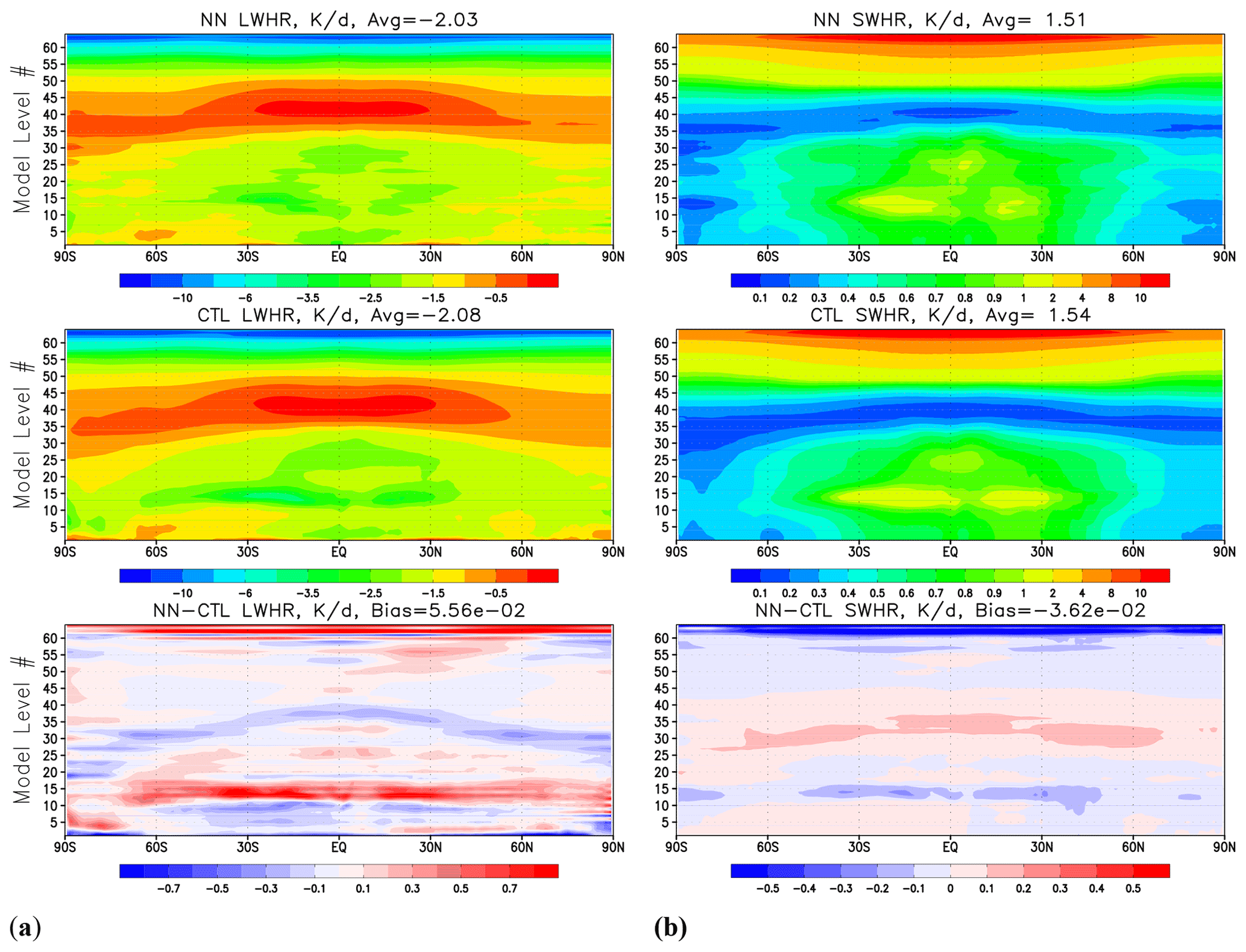
Figure 1 Zonal and time mean over 12 months' worth of model output covering 1 February 2018–1 February 2019 for (a) longwave heating rate (K d⁻¹) and (b) shortwave heating rate (K d⁻¹). Upper row – results produced by HGFS; middle – results by GFS; lower row: the difference (HGFS − GFS). The vertical coordinate shows the model level number.

Figure 1 shows zonal and time mean over 12 months' worth of model output, covering the period of 1 February 2018–1 February 2019 for LW (left panel) and SW (right panel) heating rates. Global biases are small for both heating rates and constitute about 2 %–3 % of the global mean value. A decrease in LW radiative cooling at the top of the tropical and subtropical boundary layer is compensated for by the corresponding decrease in SW radiative heating and consistent with a decrease in low cloud cover in these areas (not shown). Biases in the stratopause may be related to the new parameterizations of O₃ and H₂O photochemistry that were not present in the 2011 version of the model.

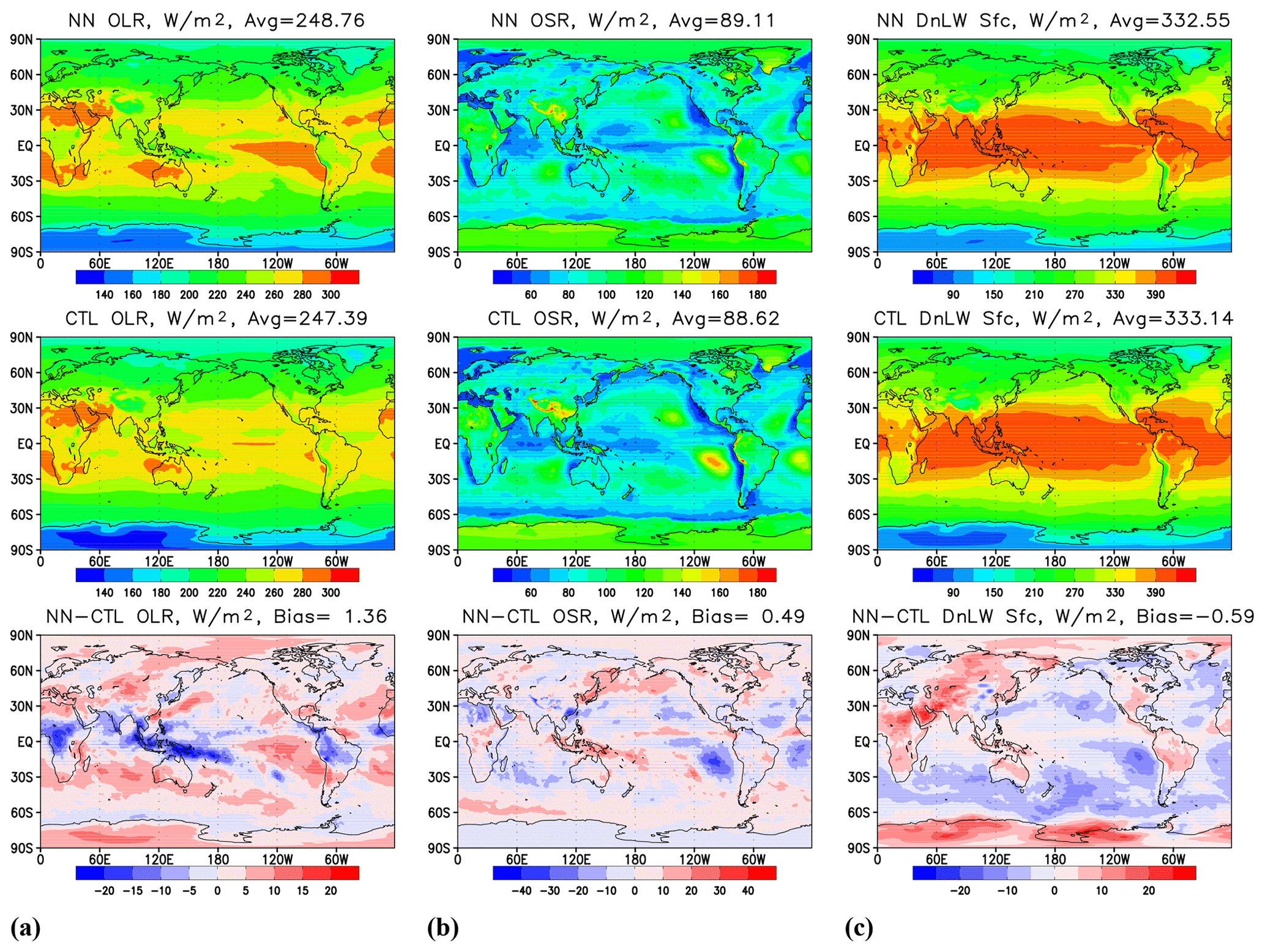
Figure 2 Time mean over 12 months' worth of model output covering 1 February 2018–1 February 2019 for (a) outgoing LW radiation at the TOA, (b) outgoing SW radiation at the TOA, and (c) downwelling SW radiation at the surface. Upper row – results produced by HGFS; middle – results by GFS; lower row: the difference (HGFS − GFS).

Figure 2a shows outgoing longwave radiation (OLR) at TOA, and panel (b) shows outgoing SW radiation (OSR) at TOA. Global biases are below 1 % of the global time mean; however, local biases are more pronounced. A decrease in OLR and increase in OSR over the Maritime Continent are consistent with an increase in high cloud cover in the region (not shown). An increase in OLR and decrease in OSR in the subtropical areas off western coasts of continents are consistent with a decrease in stratocumulus cloud cover (not shown). These changes in cloud cover are also consistent with an increase in downwelling SW at the surface in the stratocumulus regions and a decrease over the Maritime Continent, as shown in Fig. 2c, with global time mean biases being about 0.2 % of the global average.

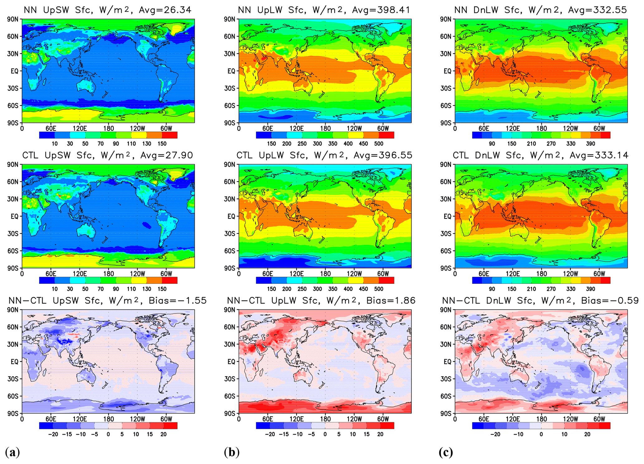
Figure 3 Time means over 12 months' worth of model output covering 1 February 2018–1 February 2019 for (a) upwelling SW radiation at the surface, (b) upwelling LW radiation at the surface, and (c) downwelling LW radiation at the surface. Upper row – results produced by HGFS; middle – results by GFS; lower row: the difference (HGFS − GFS).

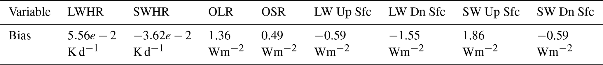
Figure 3a shows upwelling SW radiation flux at the surface. The global mean negative bias is almost 5 % of the global average value, with negative biases prevalent over continents and extratropical oceans and positive biases over tropical oceans. Upwelling LW at the surface (Fig. 3b) is biased high by about 0.5 % of the global mean value, with positive biases over most of the continents, polar areas, and most of tropical oceans and negative biases in the midlatitude oceans, northern Canada, and Alaska, as well as the Barents and Norwegian seas. Downwelling LW at the surface (Fig. 3b) is biased low globally by approximately 0.5 %. Table 2 summarizes time and global mean biases for the heating rates and radiative fluxes predicted by the emulators.

Figure 4 shows time series of a 10 d running mean of globally averaged LW and SW fluxes at the surface and the TOA generated by HGFS (black curves) and GFS (green curves) for the last 6 months (1 February–1 August) of a 7-month-long run initialized on 1 January 2018. Time series of the same quantities for the run initialized on 1 July 2018 exhibit similar properties and are therefore not shown. Magnitudes and signs of biases of each emulator-predicted variable are consistent with their time and globally averaged values shown in Table 2. The HGFS run captures the seasonal cycle and amplitude of seasonal and sub-seasonal variability reasonably well. As to be expected from long-term free-running experiments with a GCM, details of individual weather systems differ between the two runs even when considered through the lens of a 10 d running mean. This is manifested most starkly in shortwave fluxes leaving the atmosphere, outgoing SW at TOA (Fig. 4b), and downwelling SW at the surface (Fig. 4d), which are very sensitive to the instantaneous cloud distributions.

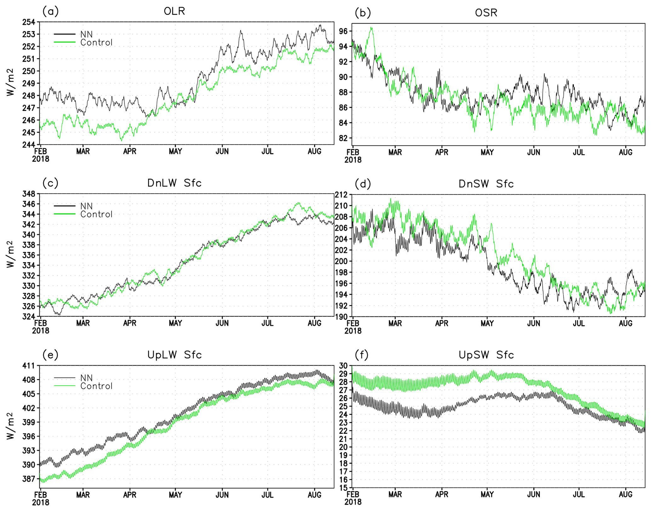
Figure 4 Time series of a running 10 d mean covering 1 February–1 August 2018 for (a) outgoing LW at TOA, (b) outgoing SW at TOA, (c) downwelling LW radiation at the surface, (d) downwelling SW radiation at the surface, (e) upwelling LW radiation at the surface, and (f) upwelling SW radiation at the surface. Black curves – results produced by HGFS; green – results by GFS.

Table 2 Time mean and global mean biases in LW heating rate (LWHR), SW heating rate (SWHR), and upwelling (Up) and downwelling (Dn) radiative fluxes at TOA and at the surface (Sfc) over 12 months' worth of model output covering 1 February 2018–1 February 2019.

5 Discussion

What could be the factors contributing to the stability of the emulators presented in this paper? In the following, we highlight and discuss aspects of the machine learning technique choice (shallow vs. deep neural network, activation function selection) and training set design that distinguish the emulators developed in Krasnopolsky et al. (2010).

5.1 Shallow vs. deep neural networks: complexity and nonlinearity

Application of shallow NNs (SNNs) to the problem of mapping approximation has thorough theoretical support. The universal approximation theorem proves that an SNN is a generic and universal tool for approximating any continuous or almost continuous mappings under very broad assumptions and for a wide class of activation functions (e.g., Hornik et al., 1990; Hornik, 1991). Similarly broad results for deep NNs (DNNs) do not exist yet (Vapnik, 2019); however, specific combinations of DNN architectures and activation functions have theoretical support (e.g., Leshno et al., 1993; Lu et al., 2017; Elbrachter et al., 2021). Until there is a universal theory, it has been suggested to consider DNN a heuristic approach since, in general, from a theoretical point of view, a deep network cannot guarantee a solution of any selection problem that constitutes a complete learning problem (Vapnik, 2019). These considerations are important to keep in mind when selecting NN architecture for the emulation of model physics or their components.

Next, we compare some properties of DNNs and SNNs to further emphasize their differences and to point out some properties of DNNs that may lead to instabilities in deterministic models coupled to DNN-based model components.

To avoid overfitting and instability, the complexity and nonlinearity of the approximating and/or emulating NN should not exceed the complexity and nonlinearity of the mapping to be approximated. A measure of the SNN complexity can be written as (see below for explanation)

$$\begin{array}{}\text{(2)}& C_{\mathrm{SNN}}=k\cdot \left(n+m+\mathrm{1}\right)+m,\end{array}$$

where n and m are the numbers of SNN inputs and outputs, and k is the number of neurons in a single hidden layer. The complexity of the SNN (Eq. 2) increases linearly with the number of neurons in the hidden layer, k. For given numbers of inputs and outputs there is only one SNN architecture or configuration with a specified complexity C_SNN. For the DNN complexity, a similar measure of complexity can be written as (again, see below for explanation)

$$\begin{array}{}\text{(3)}& C_{\mathrm{DNN}}={\sum }_{i=\mathrm{0}}^K{k}_{i+\mathrm{1}}\left(k_i+\mathrm{1}\right),\end{array}$$

where k_i is the number of neurons in the layer i (i=0 and i=K correspond to the input and output layers, respectively). The complexity of the DNN (Eq. 3) increases geometrically with the increasing number of layers, K.

Both C_SNN and C_DNN are simply the numbers of parameters of the NN that are trained or fit during SNN and/or DNN training. While there is a one-to-one correspondence between the SNN complexity, C_SNN, and the SNN architecture, given the fixed number of neurons in the input and output layers, correspondence between the DNN complexity, C_DNN, and the DNN architecture is multivalued: many different DNN architectures and/or configurations have the same complexity C_DNN given the same size of input and output layers. Overall, controlling the complexity of DNNs is more difficult than controlling the complexity of an SNN.

For an SNN given by the expression

$$\begin{array}{}\text{(4)}& y_j=b_j^{\mathrm{1}}+\sum _{i=\mathrm{1}}^k{a}_{ji}^{\mathrm{1}}\cdot t_i,j=\mathrm{1},\mathrm{\cdots },m,\end{array}$$

where n, m, and k are the same as in Eq. (2), and nonlinearity increases arithmetically or linearly with the addition of each new hidden neuron, $t_i=\mathit{\varphi }\left(b_i^{\mathrm{0}}+{\sum }_{s=\mathrm{1}}^n{a}_{\mathrm{is}}^{\mathrm{0}}\cdot x_s\right)$, to the single hidden layer of the NN.

For a DNN, symbolically written as

$$\begin{array}{}\text{(5)}& \begin{array}{rl}\mathit{Y}& ={\mathit{X}}^{n+\mathrm{1}}={\mathit{B}}^n+{\mathit{A}}^n\cdot \mathit{\varphi }\left({\mathit{B}}^{n-\mathrm{1}}+{\mathit{A}}^{n-\mathrm{1}}\right.\\ & \left.\cdot \mathit{\varphi }\left({\mathit{B}}^{n-\mathrm{2}}+{\mathit{A}}^{n-\mathrm{2}}\cdot \mathit{\varphi }\left({\mathit{B}}^{n-\mathrm{3}}+\mathrm{\cdots }\mathit{\varphi }\left({\mathit{B}}^{\mathrm{0}}+{\mathit{A}}^{\mathrm{0}}\cdot \mathit{X}\right)\right)\right)\right),\end{array}\end{array}$$

where each new hidden layer or neuron introduces additional nonlinearity on top of the nonlinearities of the previous hidden layers; thus, the nonlinearity of the DNN increases geometrically with the addition of new hidden layers much more quickly than the nonlinearity of the SNN. Thus, controlling the nonlinearity of DNNs is more difficult than controlling the nonlinearity of SNNs. The higher the nonlinearity of the model the more unstable and unpredictable generalization is (especially nonlinear extrapolation that is an ill-posed problem).

DNNs represent a very powerful and flexible technique that is extensively used for emulation of model physics and their components (Kasim et al., 2020). Discussion of its limitations can be found in Thompson et al. (2020). The arguments listed here are intended to point out possible sources of instability of DNNs in the models and the need for careful handling of this very sensitive tool.

5.2 Preparation of training sets

Specifics of training set design may impact the stability of the NN as well. We would like to point out a few aspects of training set preparation that, in our experience, are of relevance to the development of robust ML-based components of geophysical models.

A general rule of thumb when it comes to fitting statistical models to data is that the number of records in the training set should be at least as large as the number of model parameters or, in the context of the current discussion, as the NN complexity introduced in Sect. 5.1. As a consequence, NNs of larger complexity require larger training sets to approximate a given mapping. To use DNN as an example, as the complexity of DNN, C_DNN (Eq. 3), increases geometrically with the number of DNN layers, so does the amount of data required for the DNN training (Thompson et al. 2020).

We also find that comprehensiveness of the training set is an important contributing factor to the generalization capability of the NN. In the context of the application at hand, comprehensiveness of the training set means that it should encompass as much of the complexity of the underlying physical system as permitted by the numerical model that hosts the NN. In practice, it translates into sampling diurnal, seasonal and annual variability, and states introduced by boundary conditions, e.g., greenhouse gas and aerosol concentrations, realistic orography, and surface state. Inclusion of events of special interest, e.g., hurricanes, snow storms, droughts, and extreme precipitation events, is beneficial as well.

Care should be taken for proper sampling of the training data. For example, saving the training data set on a Gaussian longitude–latitude grid will result in overrepresentation of polar areas, and data must be resampled to get more uniform representation over the globe.

Purging and normalization of inputs and outputs are important. Constant inputs and outputs must be removed: from the standpoint of mapping emulation, constants carry no information about the input-to-output relation; however, with incorrect normalization, they may become a source of noise during training. Normalization of inputs and outputs strongly affects NN training. More specifically to the present application, if some inputs or outputs of an NN are vertical profiles of a physical variable, as is common in geophysical models, the profiles should be normalized as a whole, as opposed to as a collection of independent variables, for the NN to better capture correlations and dependencies between the levels of the profile (Krasnopolsky, 2013).

5.3 Continuously vs. not continuously differentiable activation functions

The universal approximation theorem for SNNs is satisfied for a wide class of bounded, nonlinear AFs. Note that many popular AFs used in DNN applications, e.g., variants of ReLU, do not belong to this class. However, for a specific problem of mapping approximation, it may be useful to consider additional restrictions on AFs.

If the AF is almost continuous or, in other words, has only finite discontinuities (e.g., step function), the first derivative (Jacobian) of the NN using this AF will be singular. If the AF is not continuously differentiable (e.g., ReLU), its first derivative will not be continuous (will have finite discontinuities) and neither will the NN Jacobian. Using a non-continuously differentiable NN as a model component may lead to instability, especially if the Jacobian of this component is calculated in the model. Using gradient-based optimization algorithms for training such NNs may be challenging due to discontinuities in gradients.

If the AF is monotonic, the error surface associated with a single-layer model is guaranteed to be convex, simplifying the training process (Wu, 2009). When AF approximates identity function near the origin (i.e., $\mathit{\varphi }\left(\mathrm{0}\right)=\mathrm{0}.,{\mathit{\varphi }}^{\prime }\left(\mathrm{0}\right)=\mathrm{1}$, and ϕ^′ is continuous at 0), the neural network will learn efficiently when its weights are initialized with small random values. When the activation function does not approximate identity near the origin, special care must be used when initializing the weights (Sussillo and Abbott, 2015).

It is noteworthy that the sigmoid and hyperbolic tangent AFs, popular in SNN applications, meet all aforementioned criteria. Additionally, in the context of emulation of model physics parameterizations, these AFs provide one of the lowest training losses compared to other AFs (Chantry et al., 2021).

6 Conclusions

One of the major challenges in the development of ML- and/or AI-based parameterizations for multidimensional nonlinear forward environmental models is ensuring the stability of the coupling between deterministic and statistical components. This problem is particularly acute for neural-network-based parameterizations since, in theory, generalization to out-of-sample data is not guaranteed, and, in practice, previously unseen inputs may lead to unphysical outputs of the NN-based parameterization, often destabilizing the hybrid model even in idealized simulations.

Shallow-NN-based emulators of radiative transfer parameterizations developed almost a decade ago for a state-of-the-art GCM are stable with respect to substantial structural and parametric change in the host model: when used in two 7-month-long experiments with the new model, they not only remain stable, but also generate realistic output. Two types of modifications of the host model that NN emulators cannot tolerate are the change in the model vertical resolution and the change in the number of model prognostic variables, in both cases due to alteration of the dimensionality of the phase space of the mapping (parameterization) and of the emulating NN. After the changes of this nature are introduced into the host model, NN emulators must be retrained.

We conjecture that careful control of complexity and nonlinearity of an AI or ML model component, along with comprehensiveness and realism of its training data set, are important factors contributing to both the component's generalization capability and the stability of the model hosting it.