the Creative Commons Attribution 4.0 License.
the Creative Commons Attribution 4.0 License.
 | 19 Nov 2021
NorCPM1 and its contribution to CMIP6 DCPP
Yiguo Wang
François Counillon
Noel Keenlyside
Madlen Kimmritz
Filippa Fransner
Annette Samuelsen
Helene Langehaug
Lea Svendsen
Ping-Gin Chiu
Leilane Passos
Mats Bentsen
Chuncheng Guo
Alok Gupta
Jerry Tjiputra
Alf Kirkevåg
Dirk Olivié
Øyvind Seland
Julie Solsvik Vågane
Yuanchao Fan
Tor Eldevik
The Norwegian Climate Prediction Model version 1 (NorCPM1) is a new research tool for performing climate reanalyses and seasonal-to-decadal climate predictions. It combines the Norwegian Earth System Model version 1 (NorESM1) – which features interactive aerosol–cloud schemes and an isopycnic-coordinate ocean component with biogeochemistry – with anomaly assimilation of sea surface temperature (SST) and -profile observations using the ensemble Kalman filter (EnKF).
We describe the Earth system component and the data assimilation (DA) scheme, highlighting implementation of new forcings, bug fixes, retuning and DA innovations. Notably, NorCPM1 uses two anomaly assimilation variants to assess the impact of sea ice initialization and climatological reference period: the first (i1) uses a 1980–2010 reference climatology for computing anomalies and the DA only updates the physical ocean state; the second (i2) uses a 1950–2010 reference climatology and additionally updates the sea ice state via strongly coupled DA of ocean observations.
We assess the baseline, reanalysis and prediction performance with output contributed to the Decadal Climate Prediction Project (DCPP) as part of the sixth Coupled Model Intercomparison Project (CMIP6). The NorESM1 simulations exhibit a moderate historical global surface temperature evolution and tropical climate variability characteristics that compare favourably with observations. The climate biases of NorESM1 using CMIP6 external forcings are comparable to, or slightly larger than those of, the original NorESM1 CMIP5 model, with positive biases in Atlantic meridional overturning circulation (AMOC) strength and Arctic sea ice thickness, too-cold subtropical oceans and northern continents, and a too-warm North Atlantic and Southern Ocean. The biases in the assimilation experiments are mostly unchanged, except for a reduced sea ice thickness bias in i2 caused by the assimilation update of sea ice, generally confirming that the anomaly assimilation synchronizes variability without changing the climatology. The i1 and i2 reanalysis/hindcast products overall show comparable performance. The benefits of DA-assisted initialization are seen globally in the first year of the prediction over a range of variables, also in the atmosphere and over land. External forcings are the primary source of multiyear skills, while added benefit from initialization is demonstrated for the subpolar North Atlantic (SPNA) and its extension to the Arctic, and also for temperature over land if the forced signal is removed. Both products show limited success in constraining and predicting unforced surface ocean biogeochemistry variability. However, observational uncertainties and short temporal coverage make biogeochemistry evaluation uncertain, and potential predictability is found to be high. For physical climate prediction, i2 performs marginally better than i1 for a range of variables, especially in the SPNA and in the vicinity of sea ice, with notably improved sea level variability of the Southern Ocean. Despite similar skills, i1 and i2 feature very different drift behaviours, mainly due to their use of different climatologies in DA; i2 exhibits an anomalously strong AMOC that leads to forecast drift with unrealistic warming in the SPNA, whereas i1 exhibits a weaker AMOC that leads to unrealistic cooling. In polar regions, the reduction in climatological ice thickness in i2 causes additional forecast drift as the ice grows back. Posteriori lead-dependent drift correction removes most hindcast differences; applications should therefore benefit from combining the two products.
The results confirm that the large-scale ocean circulation exerts strong control on North Atlantic temperature variability, implying predictive potential from better synchronization of circulation variability. Future development will therefore focus on improving the representation of mean state and variability of AMOC and its initialization, in addition to upgrades of the atmospheric component. Other efforts will be directed to refining the anomaly assimilation scheme – to better separate internal and forced signals, to include land and atmosphere initialization and new observational types – and improving biogeochemistry prediction capability. Combined with other systems, NorCPM1 may already contribute to skilful multiyear climate prediction that benefits society.
- Article
(40468 KB) - Full-text XML
-
Supplement
(22013 KB) - BibTeX
- EndNote


Retrospective predictions have demonstrated potential of forecasting seasonal-to-decadal climate variations. Particularly for the North Atlantic (Keenlyside et al., 2008; Yeager and Robson, 2017) and partly also for the North Pacific (Mochizuki et al., 2010), models show robust benefit from initializing the internal climate variability in forecasting the upper ocean state several years ahead. Prediction skill in the ocean gives rise to skill in the atmosphere and over land by affecting the atmospheric circulation or atmospheric transport of anomalous heat and moisture (Årthun et al., 2018; Athanasiadis et al., 2020; Omrani et al., 2014; Sutton and Hodson, 2005). The level of internal climate variability, and thus potential benefit from initialization, is especially high on the regional scale, where it has numerous socioeconomic applications (Kushnir et al., 2019). Comparison of initialized retrospective predictions with the observed climate evolution not only provides forecast quality information but also informs climate change attribution and Earth system model (ESM) evaluation. Initialized retrospective predictions were part of the Coupled Model Intercomparison Project phase 5 (CMIP5; Taylor et al., 2012) that provided input to the Intergovernmental Panel on Climate Change (IPCC) fifth Assessment Report (AR5) (Kirtman et al., 2013). They are also included in the latest CMIP6 (Eyring et al., 2016), as part of the Decadal Climate Prediction Project (DCPP; Boer et al., 2016), feeding into the upcoming IPCC AR6 report.
Current climate prediction systems are thought to not fully realize the predictive potential on multiyear timescales, although the practical limits of predictability themselves and their regional variations are poorly known (Branstator et al., 2012; Sanchez-Gomez et al., 2016; Smith et al., 2020). The skill of climate prediction depends on the initialization of internal climate variability state, the representation of the dynamics and processes that lead to predictability and the representation of the climate responses to external forcings (Branstator and Teng, 2010; Latif and Keenlyside, 2011; Bellucci et al., 2015; Yeager and Robson, 2017). Dynamical climate prediction systems typically use ESMs (initially developed to provide uninitialized long-term climate projections) for representing the dynamics and the responses to external forcings (Meehl et al., 2009; Meehl et al., 2014). Importantly, the dynamical prediction systems add initialization capability to the ESMs, adopting a wide range of initialization strategies (see Sect. 2.2.1) (Meehl et al., 2021). A better understanding of the three aspects – initialization, model dynamics and forcing responses – is fundamental for better exploiting the climate predictive potential and improving estimates of climate predictability (Keenlyside and Ba, 2010; Cassou et al., 2018; Verfaillie et al., 2021). The existing climate prediction systems undersample effects of model and initialization uncertainty and are not necessarily well suited to address questions related to changes in the observing system. The benefits from using advanced data assimilation for initialization, especially in an ocean density coordinate framework, are not well explored.
The Norwegian Climate Prediction Model version 1 (NorCPM1) is a new climate prediction system with coupled initialization capability that features innovations aiming to reduce initialization shock and forecast drift, and to rigorously account for observational uncertainties. NorCPM1 contributes to CMIP6 DCPP using two variants of an anomaly initialization method (see Sect. 2.2 for details), enriching the CMIP6 DCPP repository in terms of model and initialization diversity as well as simulation ensemble size. Specifically, it provides output from CMIP standard experiments (including a 30-member ensemble of no-assimilation historical simulations), two sets of DCPP coupled reanalysis simulations and two sets of initialized DCPP hindcast simulations that obtain their initial conditions from the two reanalysis sets. The output is suited for multi-model studies that address model and initialization uncertainty in climate prediction or aim at combining multiple models to achieve better predictions, and for benchmarking future versions of NorCPM.
The Norwegian Earth System Model version 1 (NorESM1; Bentsen et al., 2013; Iversen et al., 2013), the backbone of NorCPM1, has previously contributed to CMIP5 with climate projections and distinguished itself with realistic El Niño–Southern Oscillation (ENSO) variability (Lu et al., 2018) and a modest historical global warming trend that favourably compares to observations (Sects. 2.1.1 and S1 in the Supplement). It also includes a physical–biogeochemical ocean component with a vertical density coordinate and an atmosphere component with specialized aerosol–cloud schemes. While not included in this version, current development efforts are directed towards improving the regional climate representation in the sub-Arctic and Arctic and exploring benefits for climate prediction from bias-reduction techniques (Toniazzo and Koseki, 2018; Counillon et al., 2021), model parameter estimation (Gharamti et al., 2017; Singh et al., 2021), upgrades of model physics and resolution (Seland et al., 2020), improved ocean biogeochemistry (Tjiputra et al., 2020) and coupling of multiple ESMs (Shen et al., 2016).
NorCPM1 further stands out in that it uses an ensemble Kalman filter (EnKF; Evensen, 2003) based anomaly DA scheme that updates unobserved variables in the ocean and sea ice components (currently, a DA update is not applied to atmosphere and land) by utilizing the state-dependent covariance information derived from the simulation ensemble, and it also has a rigorous treatment of observation measurement and representation errors (see Appendix A for more information on the choice of DA scheme). To date, few climate prediction systems use assimilation schemes of similar complexity, and their implementations differ significantly from the one used here (see Sect. 2.2.3 for details). NorCPM's DA capability is subject to continuous development, and the system serves as a tool and testbed for new science innovations in the field of DA. Reliable ensemble prediction requires an accurate representation of uncertainty in the initial conditions and the EnKF provides a mean to achieve this. The EnKF further allows assimilation of raw observations of various types and controls the assimilation strength depending on observational error, their spatial coverage and evolution of the covariance with the state of the climate. In a Monte Carlo manner, it propagates uncertainty from the previous assimilation, providing a complete spatiotemporal uncertainty estimate. The method generates a spread in hindcast initial conditions that reflects uncertainties in the initial conditions, which typically evolve in time and space as the observational network changes. This makes NorCPM1 a suitable tool for assessing the impact of observation system changes on climate prediction. It also limits artefacts due to over-assimilation of sparse and uncertain observations in the early instrumental era. By utilizing initial conditions from a coupled reanalysis that assimilates observational anomalies into the same ESM as that used in the predictions, the system reduces initialization shock and ensures consistency of initialization anomalies across variables and with the model dynamics.
NorCPM1 has been developed from a series of prototypes. In a perfect model framework, Counillon et al. (2014) tested EnKF anomaly assimilation of synthetic sea surface temperature (SST) observations into the low-resolution version of NorESM1 and found the system to constrain well oceanic variability in the tropical Pacific and subpolar North Atlantic. The system was successively upgraded to the medium-resolution NorESM1-ME and other features such as the use of real-world SST observations (Counillon et al., 2016; Wang et al., 2019; Dai et al., 2020), assimilation of temperature and salinity profiles (Wang et al., 2017) and optional assimilation of sea ice concentration observations with strongly coupled ocean–sea ice state update (Kimmritz et al., 2018, 2019). The version described in this paper includes further upgrades of the external forcings to comply with CMIP6, code fixes, retuning of the physics, activation of ocean biogeochemistry and modifications to the anomaly assimilation scheme. These are detailed in Sect. 2.
This paper sets out to technically describe NorCPM1 and its contribution to CMIP6 DCPP and then assess the model's fitness of purpose through a broad evaluation of its baseline climate, and climate reanalysis and prediction performance. The paper intends to inform science studies that use the model's CMIP6 DCPP output, to provide a synthesis of past model development and to serve as a baseline for future development. While presenting a comprehensive reference of NorCPM1, the paper is organized in a way that makes it easy to navigate through for readers with focused interest.
The following section describes the ESM component, assimilation scheme and CMIP6 simulations performed with NorCPM1. Section 3 evaluates the reanalysis and hindcast performance of NorCPM1. Section 4 further discusses the results and related caveats. Section 5 summarizes and concludes the paper.
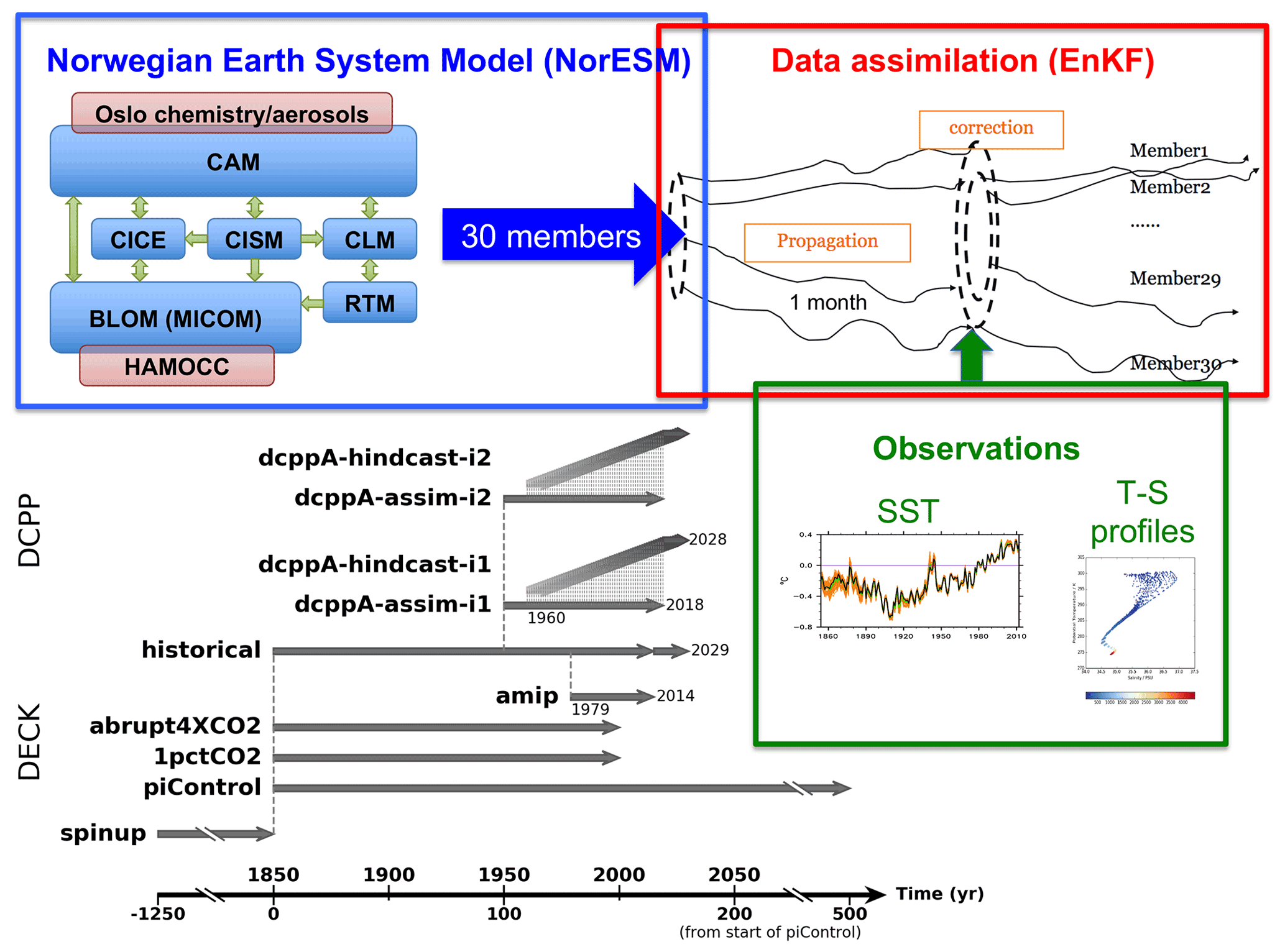
This section describes the physical model, DA approach and simulations produced for CMIP6. The prediction setup and simulations are summarized in a schematic diagram in Fig. 1.
2.1 Norwegian Earth System Model (NorESM)
The Earth system model used in NorCPM1 builds on the medium-resolution NorESM1-ME that includes a complete carbon cycle representation, which allows the model to be run fully interactively with prescribed CO2 emissions. However, we use prescribed atmospheric greenhouse gas concentrations in NorCPM. While previous NorCPM prototypes (e.g. Counillon et al., 2014, 2016) used the original CMIP5 version, NorCPM1 uses a modified version that has been subject to CMIP6 forcing updates, minor code changes and retuning (see Sect. 2.1.3). In the following subsections, we will summarize the main features of the original NorESM1-ME and then detail the differences to the version used in NorCPM1.
2.1.1 General description
NorESM1-ME (Bentsen et al., 2013; Tjiputra et al., 2013) is based on the Community Earth System Model (CESM1.0.4; Hurrell et al., 2013). Its atmosphere component CAM4-OSLO replaces the original prescribed aerosol formulation of the Community Atmosphere Model (CAM4; Neale et al., 2010) with a prognostic aerosol life cycle formulation using emissions and new aerosol–cloud interaction schemes (Kirkevåg et al., 2013). It also uses a different ocean component – the Bergen Layered Ocean Model (BLOM, formerly NorESM-O; Bentsen et al., 2013; Danabasoglu et al., 2014) – that originates from the Miami Isopycnic Coordinate Ocean Model (MICOM; Bleck and Smith, 1990; Bleck et al., 1992). The vertical density coordinate of the ocean component minimizes spurious diapycnal mixing, improving conservation and transformation of tracers and water masses. BLOM transports biogeochemical tracers of the ocean carbon cycle component – the Hamburg Ocean Carbon Cycle model (HAMOCC; Maier-Reimer et al., 2005) – which has been coupled to the physical ocean model and optimized for the isopycnic-coordinate framework (Assmann et al., 2010; Tjiputra et al., 2013). The Community Land Model (CLM4; Lawrence et al., 2011) and the Los Alamos Sea Ice Model (CICE4; Bitz et al., 2012), with five thickness categories and the elastic–viscous–plastic rheology (Hunke and Dukowicz, 1997), are adopted from CESM in their original form.
The atmosphere and land components are configured on NCAR's finite-volume 2∘ grid (f19), which has a regular latitude–longitude resolution. The atmospheric component comprises 26 hybrid sigma–pressure levels extending to 3 hPa. The ocean and sea ice components are configured on NCAR's gx1v6 horizontal grid, which is a curvilinear grid with the northern pole singularity shifted over Greenland and a nominal resolution of 1∘ that is enhanced meridionally towards the Equator and both zonally and meridionally towards the poles. The ocean component comprises a stack of 51 isopycnic layers, with a bulk mixed layer representation on top consisting of two layers with time-evolving thicknesses and densities.
2.1.2 CMIP6 forcing implementation
This section details the CMIP6 external forcing implementation into NorCPM1. Special note is made where the model setup deviates from the CMIP6 protocol. The updates of external forcing from CMIP5 to CMIP6 are expected to moderately alter the model's climate mean state, variability and anthropogenic trends. A detailed assessment of the impacts of the individual forcing upgrades is beyond the scope of this overview paper and needs to be addressed in separate studies.
The update that most affects the anthropogenic climate trend in NorCPM1 compared to the original NorESM1-ME is likely the change in anthropogenic emissions of aerosols and aerosol precursors (see Sect. 2.1.1 in Kirkevåg et al., 2013, for details of NorESM1-ME's CMIP5 aerosol implementation and emission datasets). We updated the emissions of SO2, SO4, fossil fuel and biomass burning of black carbon (BC) and organic matter (OM) to the CMIP6 pre-industrial and historical forcing (Hoesly et al., 2018). We used the Shared Socioeconomic Pathway (SSP) 2-4.5 scenario forcing, i.e. the “middle-of-the-road” scenario of the SSP2 socioeconomic family, with an intermediate 4.5 W m−2 radiative forcing level by 2100 (Gidden et al., 2019) for the post-2014 period in accordance with the DCPP protocol (Boer et al., 2016). BC emissions from aviation, omitted in the CMIP5 implementation, are now included. The representations of natural aerosol emissions of biogenic OM and secondary organic aerosol (SOA) production, dimethyl sulfide (DMS), tropospheric background SO2 from volcanoes, mineral dust and sea salt are kept unchanged.
We updated prescribed atmospheric greenhouse gas concentrations (except ozone) to Meinshausen et al. (2017) for the pre-industrial and historical period and to SSP2-4.5 (Gidden et al., 2019) for the post-2014 period. We applied globally uniform concentrations of the five equivalent greenhouse gas species (CO2, NH4, N2O, CFC-11 and CFC-12). The forcing data are at annual resolution and linearly interpolated between years by the model. Due to a bug in the merging of historical and future scenario forcing, values for 2015 and 2016 were erroneously set to 2014 values, while from 2017 all values correctly follow the scenario forcing. This results in a CO2 concentration error of less than 4 ppm, which has a negligible impact on the radiative forcing evolution but may impact ocean–atmosphere CO2 flux prediction.
We updated prescribed atmospheric ozone concentrations to Hegglin et al. (2016) (see also Checa-Garcia et al., 2018) for the pre-industrial, historical and post-2014 periods. After most simulations had been completed, we discovered that the date in our historical and post-2014 ozone input files was erroneously shifted by 23 months (e.g. the January 2000 observation is applied in February 1998). As a result, the model anticipates anthropogenic ozone changes approximately 2 years too early. The 1-month shift in the seasonal cycle may have dynamical implications particularly for the stratosphere if compared against the pre-industrial simulation that does not contain the shift.
We updated the solar forcing to the CMIP6 product (Matthes et al., 2017) as well as the stratospheric volcanic forcing (Revell et al., 2017; Thomason et al., 2018). In NorESM1-ME used in CMIP5, stratospheric volcanic aerosol loadings were prescribed, and the model then computed the resulting radiative forcing assuming certain aerosol properties and particle growth. In CMIP6, pre-computed optical parameters are provided instead and prescribed directly to the radiation code of the models in order to reduce inter-model spread in responses. NorCPM1 prescribes a zonally uniform space–time-varying extinction coefficient, single scattering albedo and hemispheric asymmetry factor for 14 solar (i.e. shortwave covering infrared, visible and ultraviolet) and 16 terrestrial (i.e. thermal longwave) wavelength bands. Despite significant changes between volcanic forcing implementations, we found only minor differences when comparing the radiative forcing to the 1991 Mt. Pinatubo eruption, with the CMIP6 implementation producing a less distinct peak and a wider tail compared to the CMIP5 implementation (not shown). Additionally, the CMIP6 experimental protocol now requires the use of a stratospheric volcanic background forcing (monthly climatology computed from historical 1850–2000 volcanic forcing) during pre-industrial and future eras, whereas the use of such background forcing was optional in CMIP5 and not implemented in the original NorESM1-ME.
We updated the land surface types and transient land use to be consistent with the Land-Use Harmonization version 2 (LUH2) dataset (Lawrence et al., 2016). For the post-2014 period, NorCPM1 deviates from the DCPP protocol as it uses land-use data from SSP3-7.0 scenario (which were the only LUH2-version land-use scenario data for CLM4 available to us at that time) instead of the recommended SSP2-4.5. For CMIP6 DCPP, the main interest is in the historical period (1850–2014). From the future scenario, only the period prior to 2030 is of interest for DCPP decadal outlooks, during which time the differences between the SSP scenarios are still small. We expect this deviation to have a minimal impact on the outcomes of NorCPM1's near-future climate outlooks (note that the greenhouse gas concentrations still follow the SSP2-4.5 scenario). Data users who specifically investigate near-future land-use-related climate feedbacks are, however, advised to either exclude NorCPM1 from their analysis or take the land-use differences between SSP2-4.5 and SSP3-7.0 into consideration. A supporting simulation experiment revealed that the update to LUH2 caused an unrealistic land–cryosphere cooling trend over the historical period in NorCPM1 (Fig. S3, S4 and text in Sect. S1 in the Supplement). The cause and ramifications are subject to further investigation.
Other forcings not mentioned above (e.g. nitrogen deposition) are kept the same as in the CMIP5 model setup.
2.1.3 Code changes, retuning and equilibration
This section describes code changes unrelated to forcing upgrades and retuning of NorCPM1 relative to NorESM1-ME that was necessary due to forcing and code changes.
An error in the aerosol code that caused an overestimation of the BC load was identified in NorESM1-ME and a correction has been proposed (details in Graff et al., 2019). The correction of this error is applied in NorCPM1 and causes a slight cooling of the climate with a −0.5 ∘C difference in the Arctic (Fig. S4).
NorESM1-ME featured too-thick sea ice on the shelf seas of the eastern Eurasian Arctic due to spurious variability in ocean velocities enhancing ice formation in the region (Seland and Debernard, 2014; Graff et al., 2019). Increasing the built-in velocity damping applied to shallow ocean regions in MICOM reduces the regional thickness bias in NorCPM1.
NorESM1-ME's ocean biogeochemistry output has been subject to substantial grid noise. The noise was traced back to a local tracer mass correction that was applied because surface freshwater fluxes do not change the ocean column mass in the model. For instance, a positive surface freshwater flux into the ocean – assuming tracer concentrations of this flux to be zero – will reduce the ocean tracer concentrations. Without a compensating increase in column water mass, such a reduction in concentrations inevitably leads to a reduction (i.e. non-conservation) in column-integrated tracer mass. The correction in NorESM1-ME locally scales the tracer concentrations such that the column-integrated tracer mass is conserved for each grid cell. This correction scheme has the weakness that it produces considerable spatial noise at the surface and artificial temporal variability and trends in the deep ocean. These problems are mitigated in NorCPM1 by replacing the local scaling with a global scaling (i.e. the same correction scale factor is used for all grid cells) that enforces global instead of local tracer conservation.
Using the original parameter settings of NorESM1-ME, the surface climate of the physical component of NorCPM1 drifts towards an unrealistic cold state with exacerbated biases as a consequence of introducing stratospheric background volcanic forcing, changing the land surface boundary conditions and correcting the bug in the aerosol code. To avoid a deterioration of climate performance and to re-equilibrate the climate, we therefore retuned NorCPM1 relative to NorESM1-ME. Specifically, we increased the condensation threshold for low clouds (from 90.05 % to 90.08 %) and also decreased the snow albedo over sea ice by adjusting parameters that affect snow metamorphosis (from r_snw = 0, dt_mlt_in = 1.5, rsnw_mlt_in = 1500 to r_snw=-2, dt_mlt_in=2.0, rsnw_mlt_in = 2000).
After the retuning, NorCPM1 neither shows obvious climate improvements nor global-scale deterioration compared to NorESM1-ME, though some regional differences exist (see Sect. S1). Since the model characteristics did not substantially change, we performed only a short pre-industrial spin-up of 250 years for NorCPM1 – using the year-1000 state of NorESM1-ME's spin-up (corresponding to the year-100 state of its CMIP5 pre-industrial control simulation) as initial conditions – in order to allow the upper ocean, sea ice and land surface to equilibrate to the model code and forcing changes.
2.2 Data assimilation (DA)
The decadal hindcasts are initialized from two coupled reanalyses of NorCPM1 in which monthly anomalies of SST and of hydrographic profiles are assimilated into NorESM using anomaly EnKF DA over the period 1950–2018. The same ESM is used for generating the reanalysis and performing the decadal hindcasts, limiting adjustments that occur after the model system is initialized. The following subsections will present the assimilated data, the DA method, its general implementation and the treatment of ocean biogeochemistry during assimilation. A rationale behind the choice of the DA method is presented in Appendix A.
2.2.1 Assimilated data
For the period 1950–2010, SST data are taken from the Hadley Centre Sea Ice and Sea Surface Temperature dataset (HadISST2.1.0.0; John Kennedy, personal communication, 2015; and Nick Rayner, personal communication, 2015) that has also been utilized in the construction of the coupled reanalysis CERA-20C (Laloyaux et al., 2018). HadISST2 provides 10 realizations of monthly gridded SST over 1850–2010 with a 1∘ resolution. The spread between the realizations, which depends on time and space, is designed to reflect uncertainties in gridding and combining SST in situ observations, retrievals from AATSR (Advanced Along-Track Scanning Radiometer) reprocessing and AVHRR (Advanced Very High Resolution Radiometer) retrievals. We consider the average and variance of these 10 realizations as the observations and their error the variance. We use monthly SST data from the National Oceanic and Atmospheric Administration (NOAA) Optimum Interpolation SST version 2 (OISSTV2; Reynolds et al., 2002) for the period 2011–2018, when HadISST2 data are not available. OISSTV2 provides weekly SST and weekly observation error variance, in addition to monthly SST. The observation error variance of the monthly data is estimated as the harmonic mean of weekly error variances provided by OISSTV2. We have confirmed through a separate reanalysis and set of hindcasts overlapping between 2006 and 2010 that the transition from HadISST2 to OISSTV2 does not cause discontinuities nor a significant change of prediction skill (not shown). SST data in the regions covered by sea ice are not assimilated; these regions are identified using the sea ice mask in HadISST2 or OISSTV2.
Subsurface ocean temperature and salinity hydrographic profile observations are taken from the EN4 dataset (EN4.2.1; Good et al., 2013). The EN4 dataset consists of profile data from all types of ocean profiling instruments, including those from the World Ocean Database, the Arctic Synoptic Basin Wide Oceanography project, the Global Temperature and Salinity Profile Program and Argo. The EN4 profile data are available from 1900 to the present, including data quality information and bias corrections (Gouretski and Reseghetti, 2010). Data that lie within the mixed layer of NorCPM's first ensemble member are not assimilated in order to maximize the impact of SST assimilation in the mixed layer. The uncertainty of observed hydrographic profiles is not available, and we have used the estimate provided by Levitus et al. (1994a, b) and Stammer et al. (2002).
2.2.2 DA method
The EnKF (Evensen, 2003) is an advanced, ensemble-based and recursive DA method. One advantage of the EnKF is its probabilistic nature that provides model uncertainty quantification through Monte Carlo ensembles (Fig. 1; red box). Moreover, the EnKF provides multivariate and flow-dependent updates, meaning that information is propagated from the observed variables to the unobserved variables dependent on the evolving state of the climate system; this is crucial to capture shifts in regimes (Counillon et al., 2016). To work efficiently, the EnKF needs an ensemble size sufficiently large to span the model subspace dimension (Natvik and Evensen, 2003; Sakov and Oke, 2008). Localization reduces the spatial domain of influence of observation which drastically reduces the need for a large ensemble size. With the recent improvements of high-performance computing, the use of the EnKF for seasonal-to-decadal climate prediction has emerged (Zhang et al., 2007; Karspeck et al., 2013; Counillon et al., 2014; Brune et al., 2015; Sandery et al., 2020). Because NorCPM1 performs monthly assimilation updates, the numerical cost for performing the updates is small compared to the cost of integrating the model.
NorCPM1 uses a deterministic variant of the EnKF (DEnKF; Sakov and Oke, 2008). The DEnKF updates the ensemble perturbations around the updated ensemble mean using an expansion of the expected correction to the forecast. This yields an approximate but deterministic form of the traditional stochastic EnKF that outperforms the latter, particularly for small ensembles (Sakov and Oke, 2008).
2.2.3 DA implementation
In order to generate the coupled reanalysis, we assimilate in the middle of the month all observations available during that month and update the instantaneous model state. Assimilation of monthly SST data implies that the innovation (i.e. observations minus model state) compares variability of an instantaneous model snapshot with that of monthly averaged observations. An alternative has been investigated, where data have been assimilated at the end of the month comparing the monthly averaged model output with the SST data. However, the latter approach shows poorer performance for reanalysis and no improvements during prediction (Billeau et al., 2016). This suggests that comparing model snapshots with monthly data is not a critical approximation for our system.
We perform anomaly assimilation in which the climatology of the observations is replaced by the model climatology. Considering the impact of the choice of the climatology reference period on the performance of reanalysis, NorCPM1 contributes two coupled reanalysis products to CMIP6 DCPP, labelled assim-i1 and assim-i2 (see Fig. 1; Sect. 2.3 for experiment overview). In assim-i1, the climatology is defined over the reference period (1980–2010) when assimilating EN4.2.1 hydrographic profile data and HadISST2 data, but over the period 1982–2010 when assimilating OISSTV2 data (i.e. beyond 2010) because OISSTV2 was not available before 1982. The model climatology is calculated from the ensemble mean of NorCPM1's 30-member no-assimilation historical experiment (Sect. 2.3). The observed climatology for assimilating hydrographic profile data is computed from EN4 objective analysis (Good et al., 2013). In assim-i2, the climatology reference period is 1950–2010. For the hydrographic profile and HadISST2 data, the climatology is computed for the longer reference period. However, the climatology for the OISSTV2 data (i.e. after 2010) is calculated from concatenated data of HadISST2 for 1950–1981 (when OISSTV2 is not available) and OISSTV2 for 1982–2010.
Together with changing the climatology reference period, we test two versions of the DA system. Time and resource constraints prevented us from testing these two aspects separately. In assim-i1, we only update the ocean state based on oceanic observations. In this case, the system belongs to the category of weakly coupled DA system (WCDA; Penny and Hamill, 2017), where the update in the ocean component of the system only influences the other components during model integration. In assim-i2, we allow the oceanic observations to update the ocean and the sea ice components. In this case, the system is a strongly coupled DA system (SCDA), where the oceanic observations influence the sea ice component of the system both at the DA step and during the model integration. To avoid confusion with atmosphere–ocean SCDA (e.g. Penny et al., 2019), we will refer to the assim-i2 approach as OSI-SCDA (where OSI stands for “ocean–sea ice”). The OSI-SCDA approach assures a more consistent initialization across components and exploits the longer temporal coverage of oceanic observations relative to sea ice observations (see also Appendix A). To update the sea ice state, we follow Kimmritz et al. (2018), where an optimal way to update the sea ice state was identified: the EnKF updates the sea ice concentrations of the individual thickness categories, while the other sea ice state variables (volume per thickness category, top surface temperature, snow and energy of melting) are post-processed to ensure physical consistency and maximize the benefit of the updates in the sea ice concentrations. In particular, the volume of the individual sea ice category is scaled proportionally to the updated individual concentration so that the prior individual category thickness is preserved. This approach ensures that the individual thickness values remain in their prescribed range but still allow a large reduction of total ice thickness error (Kimmritz et al., 2018).
The DA scheme updates all ocean physical state variables. In an isopycnal-coordinate ocean model, the layer thickness (a time-varying ocean state variable) is by definition always strictly positive. Due to normality assumptions, the linear analysis update of the EnKF may return unphysical (negative) values. To solve this issue, we use the aggregation method proposed by Wang et al. (2016), in which we iteratively aggregate layers in the vertical until no unphysical value is returned by the EnKF. This scheme does not significantly increase the computational cost of DA but avoids the drift in heat content, salt content and mass that would otherwise be caused.
The reanalysis system uses 30 ensemble members. The ensemble size is relatively small compared to the dimension of the system. In order to limit spurious correlation caused by sampling error, we use localization (Houtekamer and Mitchell, 1998). We use the local analysis framework (Evensen, 2003) in which DA is performed for each horizontal grid cell and that uses only observations around the targeted grid cell to limit spurious correlation as ocean covariance decays with distance. This also reduces the dimension of the problem. In order to avoid discontinuity in the increment at the edge of the local domain, we use the reciprocal of the Gaspari and Cohn function (a function of the distance between observation location and the target model grid; Gaspari and Cohn, 1999) to taper observation error variance (i.e. to reduce the influence of observations). We taper innovation and ensemble perturbations with the square root of the Gaspari and Cohn function, which is equivalent to the tapering of observation error variance. The localization radius used in NorCPM1 is a bimodal Gaussian function of latitude with a local minimum of 1500 km at the Equator where covariances become anisotropic, a maximum of 2300 km in the midlatitudes and another minimum in the high latitudes where the Rossby radius is small (Wang et al., 2017).
Observation errors are assumed to be uncorrelated. For the SST product, this assumption clearly fails because the SST data are the result of an analysis. We have therefore decided to only assimilate the nearest SST data. For the observed hydrographic profile, the independence of observation errors is more plausible. The observation error for the profile is considered to be the sum of the instrumental error (defined as in Levitus et al., 1994a, b, and Stammer et al., 2002) and the representativity error accounting for the model unresolved processes and scales. As detailed in Wang et al. (2017), the representativity error is estimated offline from the innovation and the ensemble spread of the 30-member historical experiment, to ensure that the reliability of the ensemble is preserved (i.e. the truth and the ensemble members can be considered to be drawn from the same underlying probability distribution function). The profile observation error is inflated by a factor of 3 in sea-ice-covered regions where the observation climatology critical for anomaly assimilation is highly uncertain because of the lack of observations. When there are several observations falling within the same grid cell, these observations are “superobed”: all observations falling within the same grid cell are averaged and the instrumental error variance is reduced as the harmonic sum of the individual instrumental error variances (Sakov et al., 2012). Note that the representativity error term mainly relates to the capability of the model to represent the truth and is thus not reduced by the superobed technique.
As further detailed in Sect. 2.3, the initial ensemble used at the start of the reanalyses (year 1950) is branched from a 30-member historical experiment. The historical experiment was initialized in 1850 from the end of a pre-industrial spin-up simulation (Sect. 2.1.3), with initial ensemble spread being generated by adding small random noise O(10−10 K) to the ocean temperatures and then integrated for 100 years, allowing the spread to grow. This approach ensures that the initial ensemble spans sufficient spread in the interior of the ocean needed for a well-calibrated EnKF and that each member is synchronized with respect to the timing of the external forcing. To avoid an abrupt start of the assimilation, the observation error variance is inflated by a factor of 8 during the first assimilation update; every two assimilation updates, the factor is decreased by one until it reaches 1, as suggested by Sakov et al. (2012). The ensemble spread is sustained during the reanalysis using the following inflation techniques. The DEnKF (Sect. 2.2.2) limits the need for inflation to some extent. We use the moderation technique of Sakov et al. (2012) – while the ensemble mean is updated with the observation error variance, the ensemble spread is updated with the observation error variance by a factor of 4. We also use pre-screening of the observation; i.e. the observation error variance is inflated so that the analysis remains within 2 standard deviations of the forecast error from the ensemble mean of the forecasts.
2.2.4 Treatment of ocean biogeochemistry
Fransner et al. (2020) showed with perfect model predictions using NorESM1-ME that the initial state of the biogeochemical tracers has a negligible impact on the predictability of ocean biogeochemistry beyond lead year 1. During the assimilation process, the thickness of the isopycnal layers changes, while the tracer concentrations on the layers remain unchanged, meaning that we allow assimilation to change the mass at every location. However, this does not introduce a drift as long as the analysis is unbiased (i.e. the assimilation does not systematically pull the model climate in one direction). This was verified with a 10-year long twin experiment where SST from a pre-industrial control run was assimilated every month into a run with 30 members. The total change in the biogeochemical tracer mass over this period was negligible; the largest drift was found for silicate that corresponded to 0.5 % of its global mass. With this approach, the global near-surface primary production approached that of the control run, showing that there is a good potential for constraining biogeochemical variability by assimilating SST only in our model setup. This might be improved by the additional assimilation of sea ice and temperature and salinity profiles. Other studies have shown that assimilation of ocean physics improves the representation of ocean biogeochemistry (e.g. Séférian et al., 2014; Li et al., 2016).
2.3 CMIP6 simulations
Figure 1 provides a schematic overview of NorCPM1's simulations prepared for CMIP6, including their temporal coverage and initialization relations. We will base our model verification and evaluations on these simulations. They can be summarized in four groups.
The Diagnostic, Evaluation and Characterization of Klima (DECK) baseline experiments comprise a coupled control experiment with fixed pre-industrial forcings (piControl), an idealized 1 % per year CO2 increase experiment (1pctCO2), an abrupt 4 times CO2 experiment (abrupt4XCO2) and a forced atmosphere experiment with prescribed observed evolution of SST and sea ice (amip). NorCPM1's piControl features three realizations to better allow time-evolving assessment of model drift. The second and third realizations start from the same initial conditions as the first realization (taken from the end of a long spin-up) but with small random noise O(10−10 K) added to the atmospheric temperature field. amip features 10 realizations (matching the ensemble size of the decadal hindcasts) with slightly perturbed atmospheric initial states. 1pctCO2 and abrupt4XCO2 feature one realization each.
The historical experiment features 30 realizations that are used for initializing NorCPM1's assimilation experiments, for constructing the climate anomalies of the assimilation experiments and also serve as a benchmark for the initialized hindcasts. The simulations are initialized from the same restart from piControl, with ensemble spread generated by adding small perturbations to the mixed layer temperatures (details in Sect. 2.2.3). In that way, we avoid contaminating influence of model drift on the ensemble spread that would occur if the restart conditions of piControl were sampled. historical-ext extends the historical simulations from 2015 to 2029 using SSP2-4.5 scenario forcing (Sect. 2.1.2) to cover the time period of the hindcast and future outlook experiments. Hereafter, historical refers to the combined historical and historical-ext experiment.
The DCPP simulations comprise two sets of assimilation simulations (dcppA-assim), hereafter referred to as assim-i1 and assim-i2, with 30 ensemble members per set. The simulations are initialized from 1 January 1950 states of historical and integrated until 15 January 2019.
The DCPP simulations further comprise two sets of decadal hindcast simulations (dcppA-hindcast), hereafter referred to as hindcast-i1 and hindcast-i2, that each feature 10 ensemble members per start date, with one start date per year from 1960 to 2018. The 15 October states of the first 10 members of assim-i1 and assim-i2 are used to initialize corresponding members of hindcast-i1 and hindcast-i2. However, we will in the following refer to 1 November as the initialization day because the assimilation update on 15 October uses observations from the entire month of October. The hindcast simulations are integrated for a total of 123 months to cover 10 complete calendar years.
In this section, we evaluate NorCPM1's reanalysis performance (Sect. 3.1) and hindcast performance (Sect. 3.2) based on the CMIP6 output. We measure skill and skill differences with anomaly correlation coefficients (ACCs) and anomaly correlation coefficient differences (ΔACCs) (for details and discussion of the skill metrics, see Appendix B and Sect. 4). An additional evaluation of the ESM, focusing on its climatology and variability characteristics, is presented in Sect. S1.
3.1 Reanalysis performance
We evaluate the performance of the assim-i1 and assim-i2 reanalyses that span the period 1950–2018 and provide the initial conditions for the decadal hindcast experiments hindcast-i1 and hindcast-i2. The following subsections cover global assimilation statistics, the impact of assimilation on the model mean states and synchronization of variability for the different components of the climate system.
3.1.1 Global assimilation statistics
We use the innovation to monitor the performance of assimilation over time (Sakov et al., 2012; Counillon et al., 2016), which is defined as the ensemble mean of the model forecast state (at assimilation time on the observational grid) minus the observation. In combination with the ensemble spread and the observation error standard deviation, it can be used to assess the reliability of the ensemble system (Sakov et al., 2012). Ideally, the reliability is checked for each grid cell. Under an ergodicity assumption, we define global statistics based on innovation as follows:
where ai is the area of the model grid cell i where the gridded observation is located, wi is the area weight, di is the innovation, is the ensemble spread (standard deviation) of forecasts, and is the standard deviation of observation error at the grid cell i at a given time. The observations are binned onto the model grid and into 42 depth bins that are also used to bin the model data. In a perfectly reliable system, the RMSE matches , i.e. the forecast ensemble spread combined with the observational error. Figure 2 shows the time evolution of the innovation statistics for SST, ocean temperature and salinity in assim-i1 (the evolution in assim-i2 is similar to that in assim-i1 and therefore not shown).
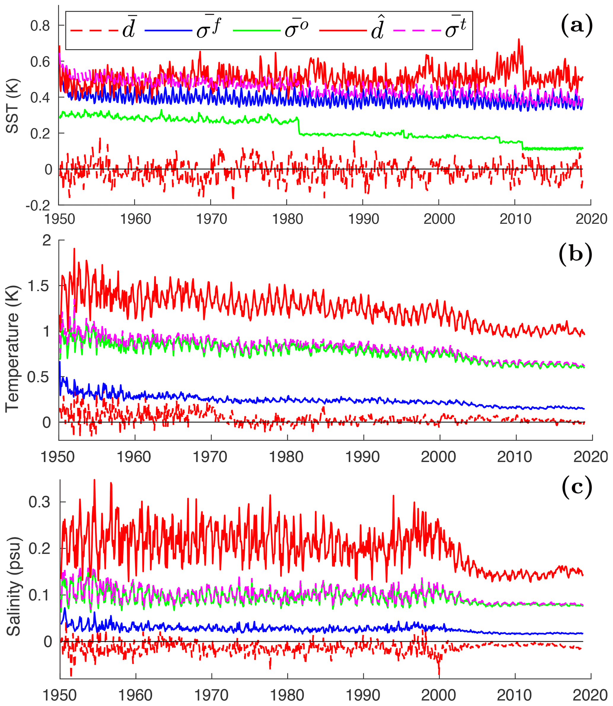
Figure 2Global assimilation statistics (see Sect. 3.1.1 for definitions). Bias (dashed red lines), ensemble spread (; blue lines), observation error (; green lines), RMSE (; solid red lines) and the total error (; pink lines) for SST (a), ocean temperature (b) and ocean salinity (c).
For SST (Fig. 2a), is stable with an accuracy of approximately 0.5 K. The bias is stable as well, fluctuating around zero. This is expected as we use anomaly assimilation (with the bias estimated from the historical experiment that does not use assimilation). It also indicates that the assimilation with a monthly cycle largely eliminates the conditional bias, caused by model error in the sensitivity to the forcing and thus corrects the forced long-term trends. The ensemble spread is also relatively stable. There is a drop in observation error standard deviation in 1982 with the emergence of satellite measurements and in 2011 with the transition from HadISST2 to OISSTV2 (see Sect. 2.2.2). The reliability of the system is good until 1982 (compare blue and magenta curves), but then drops slightly below indicating that the introduction of satellite data overly reduces the observational error estimates applied during assimilation. When the observation error reduces, the model accuracy does not increase accordingly, most likely because the model fails to represent features seen in the observations. Adding a representativity error during the satellite era to improve the reliability should be explored in future development. For ocean temperature (Fig. 2b), the RMSE decreases over time from 1.5 to 1.2 K. The bias is positive prior to 1970 but near zero afterwards. The distribution of the observations prior to 1970 is considerably uneven with a predominance in the North Atlantic region and the bias does not reflect the globally averaged bias. The total error standard deviation is smaller than the RMSE, suggesting that the ensemble system overestimates its accuracy (i.e. the ensemble spread is too small). For ocean salinity (Fig. 2c), the RMSE is stable prior to 2000 and after 2005. The decrease in the RMSE in the period 2000–2005 is due to the introduction of Argo floats. There is a negative bias in salinity prior to 2000. The bias remains negative but is relatively small after 2000. As for ocean temperature, there is a mismatch between the RMSE and total error standard deviation indicating that the system is overconfident.
3.1.2 Effect of assimilation on mean state
Anomaly assimilation should by design have a negligible effect on the climate mean state. Non-linear propagation of the assimilation updates between the assimilation updates can, however, yield a post-assimilation change in the mean state in regions where there are no observations. Furthermore, assim-i1 and assim-i2 are not using the same reference period (1980–2010 versus 1950–2010) and thus differences in the mean state can occur as because of different sampling of internal multidecadal climate variability in the observations and due to errors in the model's forced climate trend. Additionally, in the computation of observational profile anomalies, we subtracted the climatology of the objective EN4 analysis, which is inaccurate in regions with sparse data coverage. This can further impact mean states of the reanalyses.
We verify the effect of DA on the climatology by comparing mean state biases of our two assimilation products with those of the historical experiment (Fig. 3). The mean state changes due to assimilation in upper ocean temperature (T300) and salinity (S300) averaged over the top 300 m, sea surface height (SSH) and surface air temperature (SAT) are generally an order of magnitude smaller than the absolute biases of historical. The relative impact of DA on the biases is thus mostly below 10 % of its absolute magnitude. An exception is the Arctic, where the assim-i2 assimilation increases the S300 bias and decreases the SAT bias. This is consistent with that the assim-i2 assimilation tends to remove sea ice mass, leading to higher SAT because of the thinner ice and higher surface salinity because the model tries to grow back sea ice, ejecting salt during that process. Despite assimilating climate anomalies, the sea ice update in assim-i2 largely reduces the climatological sea ice thicknesses towards more realistic values, whereas the climatology of assim-i1 remains unchanged (Fig. 4). In a similar NorCPM version with climatologically too-thick Arctic sea ice, Kimmritz et al. (2019) found anomaly assimilation of observed sea ice concentration (updating the area in different thickness categories of the model using OSI-SCDA) to yield large reductions in total ice thickness error. Here, we show that similar bias reduction is achieved by a strongly coupled update of the sea ice states using ocean observations. The exact reason for this behaviour is subject to further investigation.
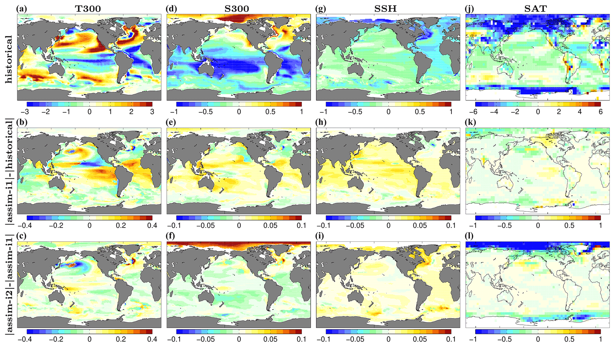
Figure 3Annual-mean climatological biases for T300 (a–c), S300 (d–f), SSH (g–i) and SAT (j–l). Biases of historical (top row), differences between absolute biases in assim-i1 and historical (middle row), differences between absolute biases in assim-i2 and assim-i1 (bottom row). Cold colours imply bias improvement. The EN4.2.1 objective analysis (Good et al., 2013) is used to estimate the biases of T300 and S300 over 1950–2018. The global 3-D thermohaline field reprocessed dataset (ARMOR-3D L4; Larnicol et al., 2006) is used to estimate the biases of SSH over 1993–2018. The Hadley Centre – Climate Research Unit Temperature dataset version 4 (HadCRUT4) (Morice et al., 2012) is used to estimate the biases of SAT over 1950–2018.
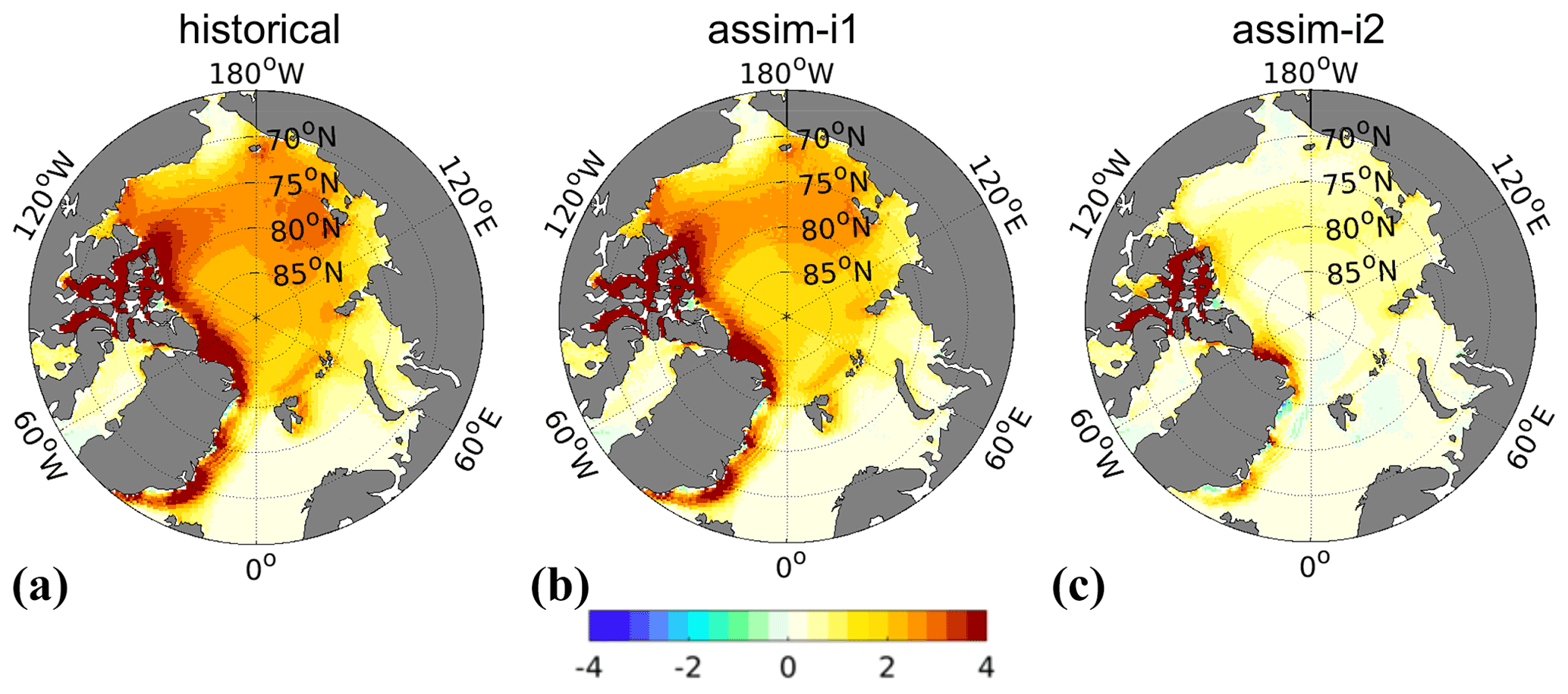
Figure 4November–March climatological biases of sea ice thickness (SIT) in historical (a), assim-i1 (b) and assim-i2 (c). The observational reference combines C2SMOS (Ricker et al., 2017), Cryosat2 (Hendricks et al., 2018a) and Envisat (Hendricks et al., 2018b) over the period 2002–2018.
The effect the assimilation has on the mean state of nutrients was assessed by investigating the difference between the ensemble means of historical and assim-i1 (Fig. 5a–c, e–g). From previous studies (While et al., 2010; Park et al., 2018), we know that the equatorial regions are the most susceptible to errors originating from assimilation of physical variables. However, since sea ice, an efficient blocker of sunlight, is updated by weakly coupled DA, some differences in the polar region are also expected. There is indeed an increase in primary production in the polar regions in the respective summers of each hemisphere. On average, there is an increase in nutrients in the Arctic, indicating that part of the increase in productivity is caused by an increase in mixing as the ocean is exposed to the atmosphere. There are very small differences in the mean nutrients in the Southern Ocean.
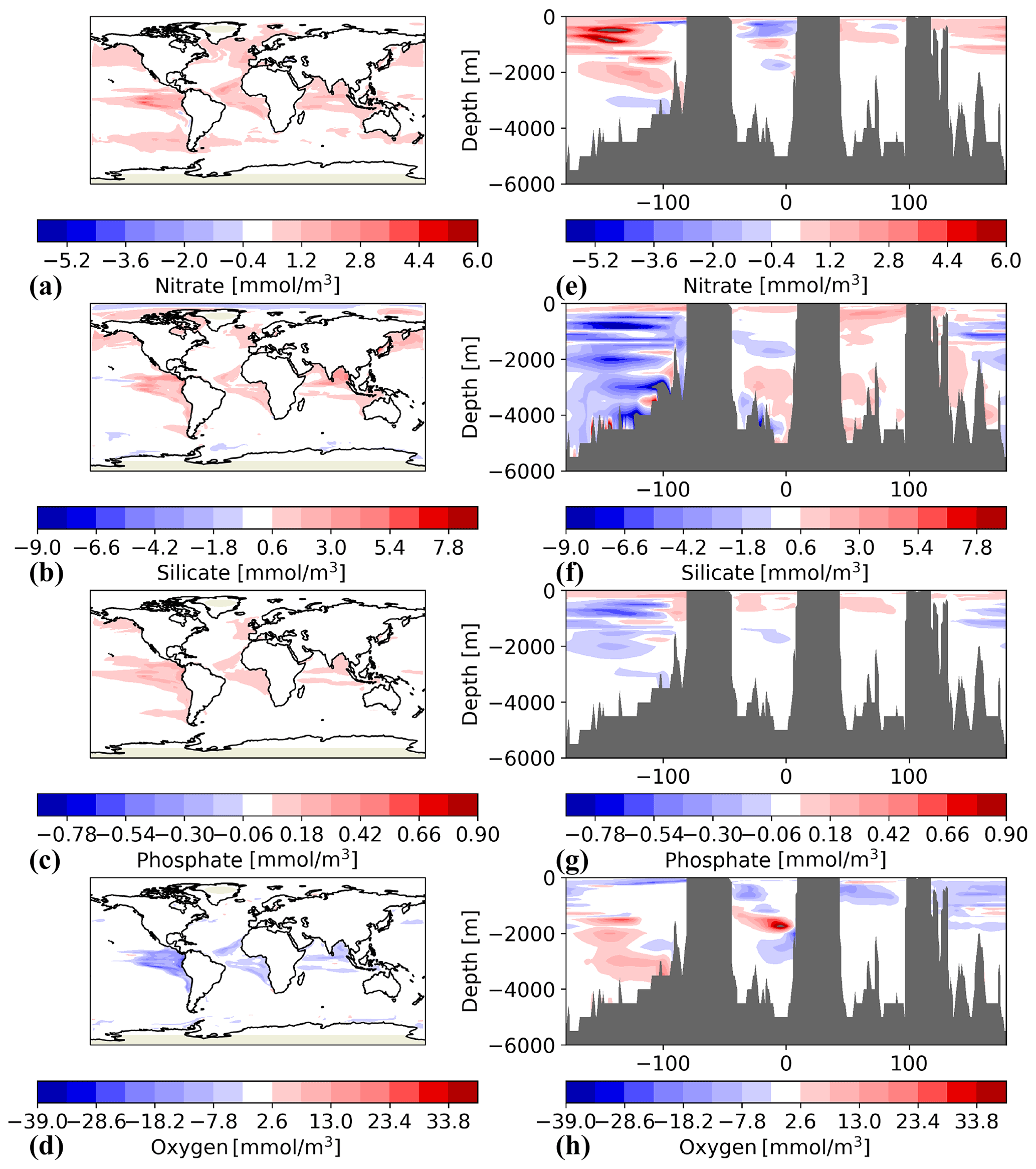
Figure 5Difference between the three nutrients – nitrate (a, e), silicate (b, f) and phosphate (c, g) – as well as oxygen (d, h) between assim-i1 and historical. Positive values means that the assimilation run has increased values. The left column shows the difference at 100 m depth and the right column shows the difference at a section along the Equator. The plots are based on the mean from the period 1950–2018.
Some impact of DA on the mean state of assim-i1 is also seen in the surface waters of the tropical oceans; these changes do not have a pronounced seasonal variation. The largest changes to the surface nitrate and phosphate occurred in the eastern Pacific, while for silicate there was also an increase in the concentration in the Bay of Bengal. The increase in silicate in the Bay of Bengal occurs throughout the water column; there is also a similar increase in the water column of the western Tropical Pacific. For nitrate and phosphate, the increase in concentration is confined to the upper 500–1000 m. At the surface and down to about 1000 m, all three nutrients have increased concentrations along the Equator. Below 1000 m, in the eastern equatorial Pacific nitrate has increased concentration, while silicate and phosphate have decreased concentrations compared to historical. An increase in nitrate with a simultaneous decrease in silicate indicates that there is some movement in the water masses that leads to decreased silicate and phosphate and at the same time an increase in oxygen in assim-i1 (Fig. 5d, h); this reduces the denitrification that occurs below the thermocline in the tropical Pacific. Furthermore, we compared the magnitude of the computed ensemble mean differences between assim-i1 and historical along the Equator with the variability of the historical ensemble. The changes are always within 1 standard deviation of the ensemble variability – i.e. small relative to the internal variability – except for oxygen in a small region at around 2000 m in the equatorial Atlantic where there is a large increase in oxygen. We therefore conclude that the changes to nutrients in assim-i1 are caused by changes to circulation and temperature and not by unphysical mixing caused by the assimilation.
3.1.3 Physical ocean variability
We first evaluate the synchronization of physical ocean variability globally at grid scale interpolated to . Figure 6 shows ACCs for annual SST, T300, S300 and SSH for assim-i1 along with ΔACCs for assim-i1 – historical and assim-i2 – assim-i1. The ACCs for assim-i1 are high and statistically significant across variables in most regions. The ΔACCs for assim-i1 – historical show that the assimilation of ocean data significantly improves the synchronization of SST, T300 and S300 with observations in most regions. Significant improvements for T300 are in the Pacific and North Atlantic. The improvements for S300 are similarly high and largest in the Arctic, albeit showing localized degradation in some coastal regions. For SSH, ACCs are increased in the subpolar North Atlantic (SPNA), tropical Pacific and Indian oceans, but decreased in the South Atlantic due to the fact that the long-term trend is degraded by the weakly coupled DA in the assim-i1 system (not shown). Missing contributions from land ice in the model possibly play a role in the degradation. The small ΔACCs for assim-i2 – assim-i1 suggest that the choice of the climatology reference period does not play an important role for the overall performance of the reanalysis in terms of variability. Significant differences appear close to the sea-ice-covered areas and are thus likely related to the sea ice state updated via OSI-SCDA in assim-i2. However, we have limited confidence in the EN4 objective analysis that we used for validation in ice-covered regions where subsurface observations are sparse.
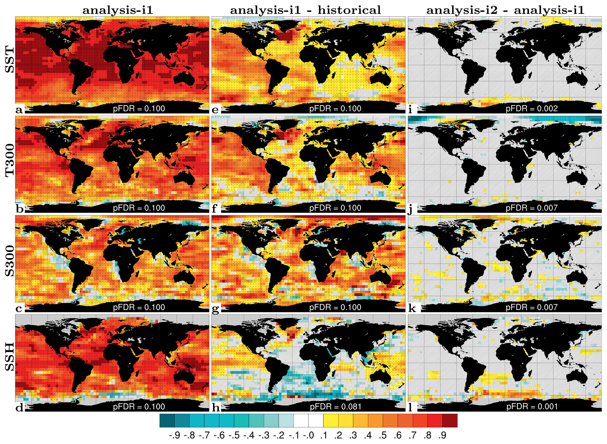
Figure 6ACC for annual SST (a), 0–300 m temperature (b), 0–300 m salinity (c) and sea surface height (d) for assim-i1. ΔACC for assim-i1 – historical (e–h), assim-i2 – assim-i1 (i–l). Temporal coverage is 1950–2018 for SST (ERSSTv5; Huang et al., 2017) and temperature and salinity (EN4.2.1; Good et al., 2013) observations, and 1993–2018 for sea surface height (ARMOR-3D; Larnicol et al., 2006). Hatched areas are not locally significant; dotted areas are field significant.
We evaluate the effect of assimilation on large-scale climate indices of leading modes of variability (Fig. 7). The North Atlantic subpolar gyre (SPG) circulation exerts strong control on subpolar North Atlantic (SPNA) temperature variations (e.g. Häkkinen and Rhines, 2004), affects the Atlantic meridional overturning circulation (AMOC) by regulating the poleward transport of Atlantic water (Hátún et al., 2005) and has a wide range of marine environmental impacts (e.g. Hátún et al., 2016). The SPG circulation index is here defined as the anomalous SSH averaged over the SPNA box (48–65∘ N, 60–15∘ W) (Lohmann et al., 2009). A positive (negative) SPG index reflects a weak (strong) barotropic mass transport in the SPNA region that usually coincides with a warm (cold) SPNA. We note that more elaborated index definitions based on principle component analysis of SSH and subsurface density are likely to capture circulation features and associated water mass variability better than our simple index (Koul et al., 2020). Figure 7a shows the SPG index over 1950–2018 in historical, assim-i1, assim-i2 and observations (altimetry data available from 1993). The observed SPG index exhibits an abrupt shift from a strong to a weak circulation around 1995, that has been linked to direct North Atlantic Oscillation (NAO) influence (Häkkinen and Rhines, 2004; Yeager and Robson, 2017) and NAO-related preconditioning of the ocean circulation state (e.g. Lohmann et al., 2009; Robson et al., 2012). The ensemble mean of the historical ensemble does not show the shift, but a slow long-term increase likely related to anthropogenic global sea level rise. The min–max range of the historical ensemble nevertheless bounds the observed SPG index, suggesting that the model range of variability is not inconsistent with the observed trajectory. The ensemble means of assim-i1 and assim-i2 show pronounced strong and weak SPG index phases and match well the observed SPG index changes during 1993–2018. Their simulated weak phase during 1950–1970 and strong phase during 1980–1997 are also in good agreement with other model studies (e.g. Msadek et al., 2014). The ensemble ranges of assim-i1 and assim-i2 are much smaller than that of historical, indicating the ensemble members are well synchronized by the assimilation. Despite showing similar decadal-scale variability, assim-i1 and assim-i2 have different means and long-term trends. The stronger SPG circulation of assim-i2 goes in tandem with a stronger AMOC, and it is likely that these two are related (Eden and Willebrand, 2001; Eden and Jung, 2001; Böning et al., 2006).
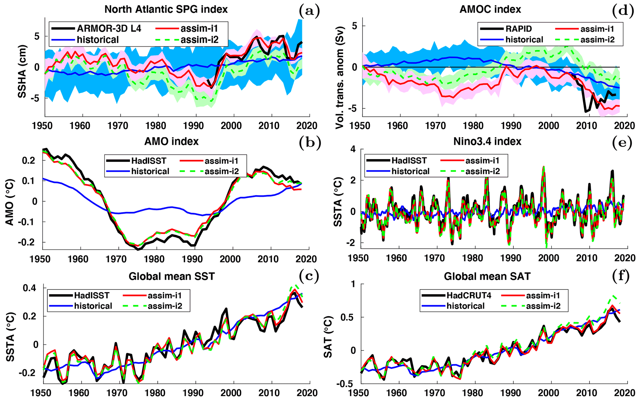
Figure 7Anomaly time series for selected large-scale indices. (a) Annual-mean subpolar gyre (48–65∘ N, 60–15∘ W) SSH with ARMOR-3D L4 observations (Larnicol et al., 2006). (b) Annual-mean AMOC strength at 26.5∘ N with RAPID observations (Johns et al., 2011). (c) Monthly Niño 3.4 index with HadISST observations (Rayner et al., 2003). (d) Atlantic Multidecadal Oscillation (AMO) index computed as the 10-year running mean of detrended SST averaged over the North Atlantic (0–65∘ N, 0–80∘ W), with HadISST observations. (e) Global-mean SST with HadISST observations (Rayner et al., 2003). (f) Global-mean SAT with HadCRUT4 observations (Morice et al., 2012). In all panels, the 1950–2018 climatology of historical is removed from historical, assim-i1 and assim-i2. Observations in panels (a) and (b) are shifted to align their time mean with assim-i1. Observations in panels (c), (d), (e) and (f) are relative to 1950–2018 climatology.
The strength of AMOC is measured continuously from April 2004 at 26.5∘ N by a joint US–UK Rapid Climate Change – Meridional Overturning Circulation and Heat flux Array (RAPID-MOCHA; Johns et al., 2011). Accordingly, we define the AMOC index as the yearly anomalies of overturning transport maximum at 26.5∘ N. Figure 7b shows the AMOC indices of historical, assim-i1 and assim-i2 and observations. The ensemble mean of historical, a measure for the simulated anthropogenic trend, rises before the mid-70s and then slowly declines. In contrast, the two assimilation products show a weakening before the mid-70s, followed by a strengthening that is consistent with a dominantly positive observed NAO during that period (Robson et al., 2012; Yeager and Robson, 2017; Zhang et al., 2019). The simulated AMOC strongly declines after 2005, though not as rapidly as in the observations, and flattens after 2010. Similar results have been shown in previous studies (e.g. Keenlyside et al., 2008; Karspeck et al., 2017). As for SPG circulation, assim-i1 and assim-i2 show similar multiyear AMOC variations but different long-term trends. Most notably, assim-i1 stays below the ensemble mean of historical over the entire period, while assim-i2 surpasses historical around 1990, which is more consistent with the anomalously strong AMOC during the mid-90s SPG shift. Results from a supporting experiment suggest that the stronger circulation in assim-i2 is primarily caused by the different climatological period but also partly by the OSI-SCDA update of sea ice (Fig. S8 and related text in Sect. S2).
The Atlantic Multidecadal Oscillation (AMO) – or Atlantic Multidecadal Variability – refers to large-scale, low-frequency SST variations in the North Atlantic, with linkages to AMOC variability (Keenlyside et al., 2015; Yeager and Robson, 2017). Following Enfield et al. (2001), we define the AMO index as the 10-year running mean of linearly detrended SSTs averaged over the entire North Atlantic (0–65∘ N, 0–80∘ W). Figure 7c shows the index in observations, historical, assim-i1 and assim-i2. In agreement with observations, the indices of all three experiments are in a warm phase during 1950–1965 and 1995–2018 and a cold phase during 1965–1995. However, the historical ensemble mean (representing the forced response of the model) underestimates the amplitude, exhibits a longer cold phase as well as an upward trend after 2010, when observations show a downward trend. As a result of assimilating SST observations, the AMO indices of assim-i1 and assim-i2 both follow the observed index with only minor departures. assim-i2 shows a slightly weaker post-2000 downward trend than assim-i1 and observations, either related to differing sea ice behaviour or differences in AMOC.
While ocean dynamics in the Atlantic basin give rise to multiyear climate predictability, ENSO variability is an important source for seasonal and interannual predictability. The ESM features realistic ENSO characteristics (Figs. S5, S6 and text in Sect. S1). But how well do monthly DA updates synchronize the model's ENSO variability with the observed one? Figure 7d shows the monthly Niño 3.4 – computed as the average of SST in the region 5∘ S–5∘ N, 120–170∘ W – for historical, assim-i1 and assim-i2 and HadISST. Both assim-i1 and assim-i2 accurately reproduce the observed index, showing a perfect match of the large 1998 event but slightly underestimate other peaks. We attribute the good performance to DA in NorCPM1 constraining well thermocline depth (equivalent to warm water volume) in the equatorial Pacific that is critical to develop ENSO events (Meinen and McPhaden, 2000; Wang et al., 2019). The Niño 3.4 indices of assim-i1 and assim-i2 are almost identical, meaning that the climatology reference period defined in anomaly assimilation and the jointly updated sea ice state have little impact on the equatorial Pacific. The ensemble mean of historical has a smaller amplitude and is only marginally correlated with the observed index (r=0.2, p=0.085, alpha = 0.1), suggesting a potential small contribution from external forcing.
Last, we consider the effect of assimilation on the global-mean SST representation. Figure 7e shows the anomalies of global-mean SST evolution for historical, assim-i1, assim-i2 and HadISST. historical captures the long-term warming trend and some shorter volcanic cooling events (e.g. after the 1963 Mt. Agung and 1991 Mt. Pinatubo eruptions). assim-i1 and assim-i2 additionally capture the high-frequency variability on top of the forced signal. The assimilation experiments show minor discrepancies with respect to observations, such as a too-weak post-eruption Mt. Pinatubo recovery and a seemingly underestimated 1998 El Niño imprint on global-mean SST. assim-i2 exhibits a slightly more positive trend after 2010 compared to assim-i1, which likely is the imprint of the more positive trend in AMO on global-mean SST. The behaviour of global-mean SAT (Fig. 7d) is similar to that of SST and will be further addressed in Sect. 3.1.6.
3.1.4 Ocean biogeochemistry variability
The correlation skills of annual-mean primary production (PP), pCO2 and air–sea CO2 fluxes for the assimilation experiments are shown in Fig. 8. For PP, the total skill (with contribution from external forcing) is high and field significant in the tropical Pacific and Indian oceans, with some skill in the subtropical oceans. The ΔACCs between assim-i1 and historical, measuring assimilation benefit, are not field significant and smaller in value than the ACCs of assim-i1, indicating that most skill comes from the external forcing. Still, large regions in the tropical Pacific and Indian oceans feature high ΔACCs that are locally significant. The ΔACCs between assim-i2 and assim-i1 are generally small. The largest differences are found in the polar regions, although precaution should be taken when evaluating the PP in these regions due to the low coverage of satellite data.
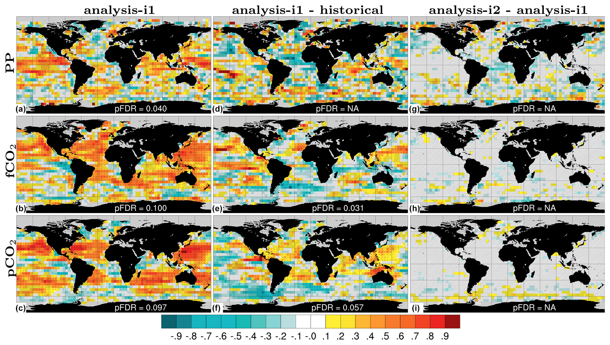
Figure 8ACC for annual primary production (a), CO2 flux (b) and surface pCO2 (c) for assim-i1. ΔACC for assim-i1 – historical (d–f), assim-i2 – assim-i1 (g–i). Temporal coverage is 1998–2018 for observed primary production (GlobColour; Garnesson et al., 2019) and 1982–2017 for CO2 flux and surface pCO2 (SOCCOM; Landschützer et al., 2019). The linear trend has been removed from the data. Hatched areas are not locally significant; dotted areas are field significant.
For the CO2 fluxes and pCO2 (linearly detrended), the total skill is high and field significant over the tropical and subtropical oceans. Exceptions are eastern part of the tropical Pacific, and the southern subtropical Pacific for the CO2 fluxes. For CO2 fluxes, there is also high skill in the southern part of the Southern Ocean and in the Nordic Seas. This is not the case for pCO2, which suggests that part of the CO2 flux skill might be related to successful synchronization of sea ice variability. As for PP, the ΔACCs relative to historical are considerably smaller than the ACCs of assim-i1, despite the linear detrending that was applied to the CO2 fields before the ACC computation. The ΔACCs remain field significant in parts of the subtropical and tropical oceans, although with a reduced westward extension of the skilful areas. Contrary to expectation, the SPNA shows little skill. As for PP, skill differences for CO2 fluxes and pCO2 are small between assim-i1 and assim-i2.
3.1.5 Sea ice variability
We evaluate the success of our assimilation in phasing sea ice variability. We use ACC maps of annual-mean sea ice concentration and HadISST (Rayner et al., 2003) data from 1950–2018 as a benchmark (Fig. 9).
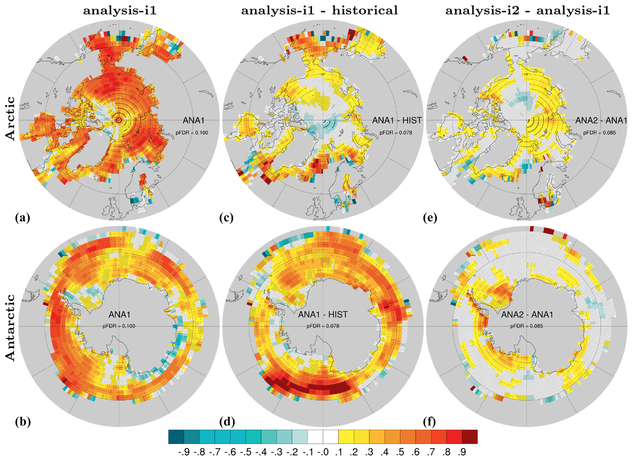
Figure 9ACC for annual sea ice concentration in Arctic (a) and Antarctic (b) for assim-i1. ΔACC for assim-i1 – historical (c–d), assim-i2 – assim-i1 (e–f). Observations are from HadISST (Rayner et al., 2003) over the period 1950–2018. The data are interpolated to a regular grid. Hatched areas are not locally significant; dotted areas are field significant.
Over the Arctic, assim-i1 features overall high skill. While much of this skill is from the externally forced trend, positive assim-i1 – historical ΔACCs show that ocean DA considerably improves the agreement in the marginal ice zones. Positive ΔACCs for assim-i2 – assim-i1 show that updating the sea ice state via OSI-SCDA of ocean observations further improves the agreement, including over the central Arctic.
Over the Antarctic, assim-i1 shows modest to high skill and only isolated negative ACCs. Strikingly, the assim-i1 – historical ΔACCs are as high or higher than the absolute ACCs of assim-i1. This means that assimilation corrects for the negative trend in the historical ensemble. OSI-SCDA again improves the skill (Fig. 9f), especially close to the coast where the ACCs of assim-i1 are low or negative (Fig. 9b).
3.1.6 Atmosphere variability
Because our DA is weakly coupled with respect to the atmosphere, we expect a partial synchronization of atmospheric variability from the combined influence of the ocean surface–sea ice states and the external forcings. The reanalysis performance provides a hypothetical upper bound for the achievable atmospheric–land prediction skill with our system, assuming close-to-perfect prediction of ocean variability and skilful prediction of sea ice variability. We assess the synchronization of atmospheric variability with ACCs of annual-mean SAT, precipitation over land (PR), sea level pressure (SLP) and 500 hPa geopotential height (Z500) for assim-i1 (Fig. 10a–d). We also consider ΔACCs for assim-i1 – historical and assim-i2 – assim-i1 to isolate skill contribution from DA and skill differences between two reanalysis products.
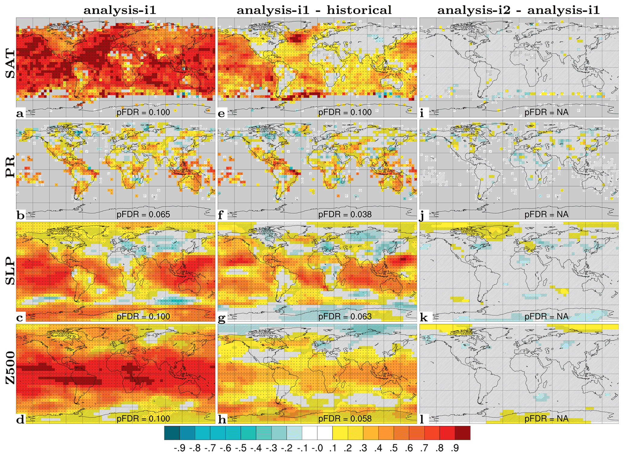
Figure 10ACC for annual 2 m temperature (SAT, a), precipitation (PR, b), sea level pressure (SLP, c) and 500 hPa geopotential height (Z500, d) for assim-i1. ΔACC for assim-i1 – historical (e–h), assim-i2 – assim-i1 (i–l). Temporal coverage is 1950–2018 for observed SAT (HadCRUT4; Morice et al., 2012), PR (CRU TS4.03; Harris et al., 2020), SLP (NCEP reanalysis; Kalnay et al., 1996) and Z500 (extended ERA5; Harris et al., 2020). Hatched areas are not locally significant; dotted areas are field significant.
For SAT, the ACCs of assim-i1 are high over both ocean and land. Most of the DA benefit is located over the oceans, as revealed by the ΔACCs for assim-i1 – historical, with benefits over land mainly found in the tropical regions and also over northwest North America, i.e. regions that are strongly affected by ENSO variability. assim-i2 does not show any significant skill improvement over assim-i1, despite the sizable improvements in sea ice variability when updating the sea ice state via OSI-SCDA. This is likely because the improvements in sea ice extent (Fig. 9) occur mostly during summer when they have little impact on surface temperatures (Deser et al., 2010). For global-scale SAT synchronization, the global warming hiatus at the beginning of the 21st century, which has been attributed to both internal variability and external forcing (e.g. Medhaug et al., 2017), makes an interesting test case. Figure 7f shows that global-mean SAT anomaly of assim-i1 reproduces well the flat post-2000 trend of the observations, while assim-i2 and historical continue to warm, consistent with their AMO and AMOC evolution. The better match of assim-i1 with observed global-mean SAT does not necessarily imply that assim-i1 is more correct than assim-i2. It is possible that assim-i1 makes up for a missing post-2000 cooling signal over the continents by an unrealistic low reduction of winter sea ice thickness during that period, something that warrants further investigation.
For PR over land, the ACCs of assim-i1 are overall positive. The ΔACCs for assim-i1 – historical show similar strength and pattern, indicating a limited contribution to the ACCs of assim-i1 from the anthropogenically driven spin-up of the hydrological cycle. The ΔACCs for assim-i2 – assim-i1 do not suggest statistically significant performance differences between the two products.
For SLP, the ACCs of assim-i1 are most positive over the low and high latitudes and less positive over the midlatitudes, with slightly negative values over the Southern Ocean and Eurasia. The ΔACCs for assim-i1 – historical suggest that a large portion of the positive skill can be attributed to DA, including benefits over the North Pacific that stretch over North America and also over the SPNA, consistent with ENSO influence. However, DA seems to cause degradation over the subtropical North Atlantic, central Europe, Siberia and East Asia. The ΔACCs for assim-i2 – assim-i1 reveal that updating sea ice improves SLP performance over the Arctic. DA also seems to partly mitigate the skill deficit over central Europe while degrading skill further east.
For Z500, the correlation skill of assim-i1 is virtually saturated over the tropics, decreases towards the midlatitudes and again slightly increases towards the poles. While modest ΔACCs for assim-i1 – historical indicate that external forcing contributes significantly to high tropical skill, DA leads to consistent skill enhancement in those regions. One should note that a change in correlation from 0.6 to 0.9 equates to more than doubling in explained variance from 36 % to 81 % (estimated by the square of the correlation). Hence, the benefit from DA is more substantial than the ΔACCs alone would suggest. Significant skill enhancement is also present over the mid-to-high latitudes, presumably related to ENSO influence on the extratropical atmospheric circulation. The ΔACCs for assim-i2 – assim-i1 indicate weak improvement over the polar regions, albeit not statistically significant, and no signs of degradation, as a consequence of updating the sea ice during DA.
3.2 Hindcast performance
This section evaluates retrospective predictions with NorCPM1 that are initialized on 1 November (i.e. no observations after 31 October are utilized in the initialization) of the years 1960–2018. We demonstrate skill benefits from forecast initialization as well as from using a dynamic prediction system. To assess skill degradation with forecast lead time, we consider the different time-averaged forecast ranges lead year 1 (LY1), lead years 2–5 (LY2–5) and lead years 6–9 (LY6–9). We compare these against the skill of NorCPM1's reanalyses, uninitialized prediction (constructed from historical) and persistence forecast (defined in Appendix B). We also highlight performance differences between the two hindcast products hindcast-i1 and hindcast-i2. The following subsections present skill evaluations for the physical ocean, marine biogeochemistry, sea ice and atmosphere.
3.2.1 Physical ocean variability – globally
SST prediction has the most direct application for near-term climate impact assessment. We evaluate NorCPM1's capability to predict interannual-to-multiyear SST variations with ACC skill maps for hindcast-i1 along with skill difference maps for hindcast-i1 – assim-i1, hindcast-i1 – persistence, hindcast-i1 – historical and hindcast-i2 – hindcast-i1 (Fig. 11). For LY1, hindcast-i1 exhibits generally positive ACCs, exceeding 0.8 over extended areas, that are both locally and field significant except for limited regions in the eastern Pacific and at high latitudes (Fig. 11a). The system loses information of the initial condition over time, resulting in notably smaller ACCs compared to the assim-i1 reanalysis (Fig. 11b). Significant benefits from initialization, as diagnosed from the ΔACC of hindcast-i1 – historical, are concentrated in the Pacific and Atlantic sectors of the tropics and Southern Ocean, and also in the subpolar North Atlantic (SPNA) and extending from there into the Eurasian Arctic (Fig. 11d). Consistent with other prediction systems (e.g. Yeager et al., 2018), the SPNA stands out as the region that benefits most from initialization. However, hindcast-i1 does not outperform persistence in the SPNA (Fig. 11c), indicating that the benefit of initialization primarily offsets poor performance of the uninitialized dynamical prediction of historical in that region. hindcast-i2 shows improved skill over hindcast-i1 in sea-ice-covered regions and in a small part of the SPNA (Fig. 11e). These skill differences are not field significant, but the fact that the two systems differ in their sea ice treatment adds confidence that skill improvements in the polar regions are real. Much of the LY1 skill, in particular in the tropics, is likely related to skilful initialization of ENSO in NorCPM (Fig. S9 and text in Sect. S2), which has been studied in detail using a similar model configuration (Wang et al., 2019).
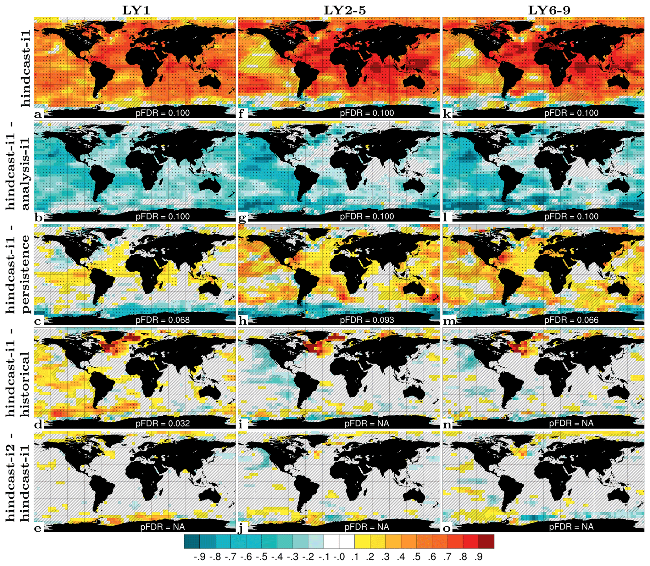
Figure 11Prediction skill for SST. ACC of hindcast-i1 (a), ΔACC of hindcast-i1 – analysis-i1 (b), ΔACC of hindcast-i1 – persistence (c), ΔACC of hindcast-i1 – historical (d) and ΔACC of hindcast-i2 – hindcast-i1 (e) for LY1. The middle and right columns show the same but for LY2–5 (f–j) and LY6–9 (k–o). Observations use ERSSTv5 (Huang et al., 2017) with coverage for 1960–2018. Hatched areas are not locally significant; dotted areas are field significant.
The LY2–5 and LY6–9 multiyear SST skill patterns (Fig. 11, middle and right columns) resemble that of LY1 but with some notable differences. Large regions in the eastern central North Atlantic, tropical Indian Ocean and western Pacific show elevated skills that exceed 0.9. The same regions show, however, negligible gains relative to uninitialized prediction of historical (Fig. 11i, n). Thus, the skill increase relative to LY1 is likely due to the forced trend having more weight, as the 4-year averaging effectively filters out interannual internal variability, and less due to the presence of more predictable internal climate variability on multiyear timescales or forecast shock that more strongly impacts LY1. Despite limited initialization benefit, the initialized predictions globally outperform persistence except for in the Southern Ocean. Since we expect the persistence forecast to capture a linear trend, this may indicate a significant skill contribution from non-linearities in the forced trend. Also for multiyear prediction, the SPNA and its extension towards the Arctic stand out as the region benefiting most from initialization, although the benefit is somewhat reduced and less statistically robust than for LY1 (Fig. 11d). Over time, the impact of initializations in the SPNA diminishes and the system drifts back to the poorly performing simulated forced trend, causing skill deficit to emerge (Fig. 11f, k). This result stands in contrast to multi-model findings (that include NorCPM1) suggesting a positive contribution of the forced signal to SPNA temperature skill over a comparable period (Borchert et al., 2021). We suspect a problem with CMIP6 land use change specification (Fig. 13c and text in Sect. S1), leading to an unrealistic historical cooling trend over North America in NorCPM1. Via downstream effects, the continental cooling (likely an artefact) may contribute to the SPNA cooling trend shown after 1980, exacerbating the discrepancy between the observed and simulated SPNA temperature evolution. The eastern Pacific presents another region where the skill notably deteriorates over time. The historical simulations perform better here than for the SPNA (Fig. 11i, n), suggesting a detrimental effect of initialization on multiyear scales on Pacific SSTs notwithstanding the positive effect on LY1 prediction. Also for multiyear prediction, hindcast-i2 performs better than hindcast-i1 in the high-latitude regions, notably in the northwestern North Atlantic (Fig. 11j, o). However, the multiyear skill hindcast-i1 – historical and hindcast-i2 – hindcast-i1 differences are both not field significant, and we thus cannot exclude that they are a sampling artefact.
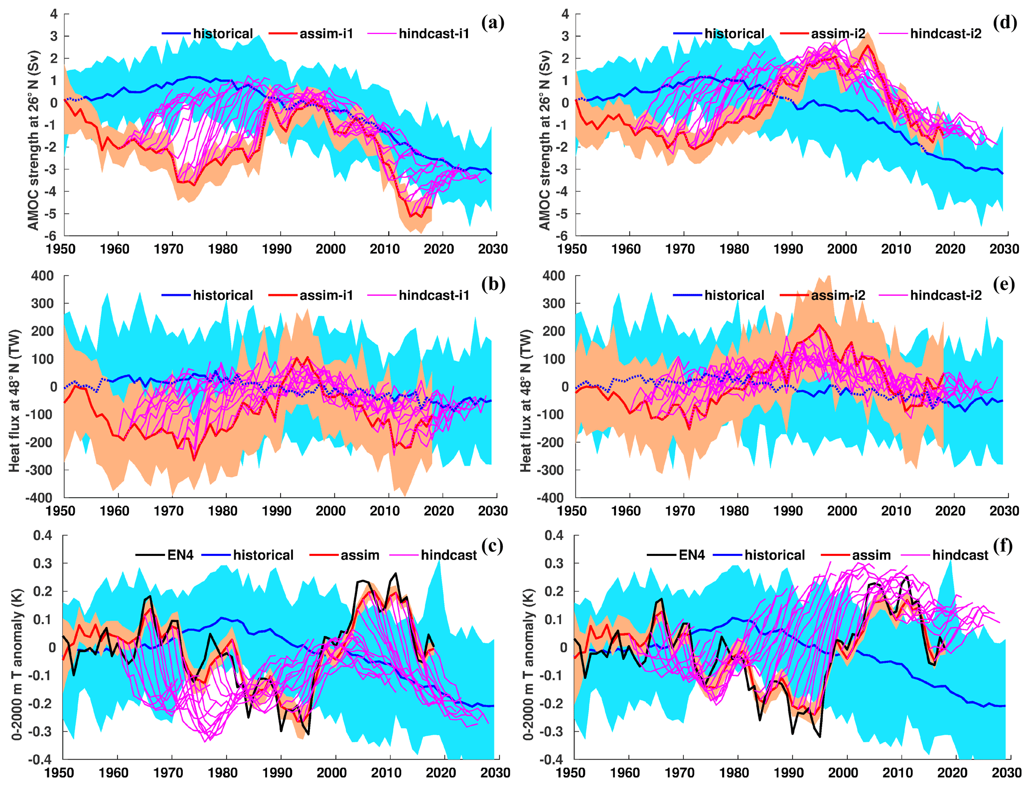
Figure 12AMOC strength at 26∘ N, Atlantic meridional ocean heat transport at 48∘ N and 0–2000 m temperature averaged over the SPNA box (48–65∘ N, 60–15∘ W) for i1 (a–c) and i2 (d–f). Solid lines show ensemble means of historical (blue), assim (red) and hindcast (purple) experiments, with the 1950–2010 average of historical subtracted. Shading denotes ensemble minima and maxima.
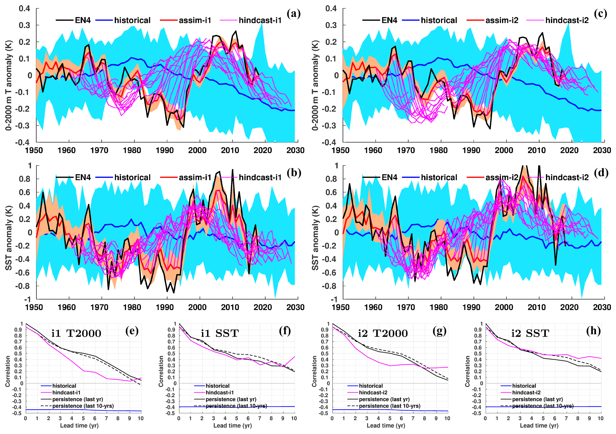
Figure 13Drift-corrected 0–2000 m temperature (T2000) and SST averaged over the SPNA box (48–65∘ N, 60–15∘ W) for i1 (a, b) and i2 (c, d), respectively. Solid lines show ensemble means of historical (blue), assim (red) and hindcast (purple) experiments, with the 1950–2010 average of historical subtracted. Shading denotes ensemble minima and maxima. Also shown are ACCs as function of lead time for T2000 and SST for i1 (e, f) and i2 (g, h), respectively. The persistence forecasts use the average over the last year (solid) and last 10 years (stippled) from the observations.
Skill patterns for the upper ocean temperature and salinity averaged over the top 300 m (Figs. S10, S11) and for sea surface height (Fig. S12) – a proxy for circulation and vertically integrated behaviour – largely reflect those for SST. Skill enhancement due to multiyear averaging is less apparent than for the surface state, presumably due to less presence of interannual climatic noise below the surface. Initialization benefit in the SPNA extends below the surface, across variables, and stands out as a robust feature.
3.2.2 Physical ocean variability – SPNA
Initialization of the large-scale ocean circulation and the associated meridional heat transport have been identified as essential for skilful prediction of SPNA climate (e.g. Yeager and Robson, 2017). We evaluate in more detail how well NorCPM1 represents mechanisms that give rise to North Atlantic decadal predictability. This evaluation provides additional forecast quality information and a better understanding of the hindcast-i2 – hindcast-i1 skill differences and of how well the predictive potential for North Atlantic SSTs is realized in the system.
The forced evolution of the AMOC strength shows a slight increase until 1980 and weakening thereafter (Fig. 12a, blue solid). assim-i1 initializes the circulation in an anomalous weak state prior to 1990, close to neutral between 1990 and 2010, and weak again thereafter (solid red), with the initial perturbations tending to be outside the internal variability range (blue shading). After initialization, the circulation (solid purple) rapidly relaxes towards the unperturbed ensemble-mean state evolution of historical (solid blue). Because ocean heat exchange between the subtropical and the SPNA covaries with the variability in AMOC strength (Fig. S13e–g), the anomalies of the northward heat transport at the time initialization (Fig. 12b, red solid) roughly resemble those of the circulation, mostly showing anomalously negative transports, except during the 1990s. The heat transport relaxes towards the ensemble-mean of historical during the hindcasts. assim-i2 shows generally stronger circulation and heat transports with weaker long-term decline than assim-i1 (Fig. 12d, e). These circulation and heat transport differences are key to explaining strikingly different SPNA temperature evolution in hindcast-i1 versus hindcast-i2 (Fig. 12c, f). hindcast-i1 and hindcast-i2 notably drift away from the observed SPNA-averaged temperature trajectory, suggesting that both configurations struggle to predict the observed decadal SPNA temperature trends. However, while hindcast-i1 exhibits drift behaviour towards cooling (most pronounced during 1960–1980 and after 2005), hindcast-i2 exhibits drift behaviour towards warming (most severe during 1980–2000).
Diagnosing the hindcast SPNA temperature evolution from the anomalous ocean heat transport across 48∘ N (Fig. S13a, c) or the regression of heat transport on AMOC (Fig. S13b, d) results in a very similar behaviour. The SPNA 0–2000 m heat content changes are well balanced by transport changes across 48∘ N and anomalous surface fluxes over the SPNA region (not shown). The latter mainly act to dampen the temperature signal, explaining the greater amplitude of the diagnosed temperature evolution. The resemblance of diagnosed and simulated hindcast evolution suggests that circulation exerts a strong control on the simulated SPNA temperature evolution and that poor SPNA prediction is largely a consequence of poor initialization of AMOC and associated poleward heat transport. Errors in the simulated externally forced AMOC trend and associated heat transport likely affect the skill as well.
How can hindcast-i1 and hindcast-i2 exhibit very different SPNA 0–2000 m temperature evolution but similar correlation skills? Applying lead-dependent drift correction largely removes the differences (Fig. 13a, c). Remaining differences hint at a slight time dependence, consistent with the somewhat different long-term trends in AMOC strength in assim-i1 and assim-i2 (Fig. 12a vs. d). In terms of ACC skill, hindcast-i2 performs marginally better than hindcast-i1 for long lead times but does not outperform persistence (Fig. 13e, g). The results for SPNA SST (Fig. 13b, d) generally resemble those for 0–2000 m temperature but look slightly more promising, with hindcast-i2 performing marginally better than persistence for long lead times (Fig. 13f, h).
3.2.3 Ocean biogeochemistry variability
We evaluated the performance of ocean biogeochemistry for PP and surface CO2 flux. Figure 14 shows maps of PP prediction skill for LY1, LY2–5 and LY6–9. While the results are patchy, some coherent patterns can be distinguished. For the total LY1 skill of hindcast-i1 (Fig. 14a), ACCs are relatively high and the field is significant over large parts of the tropical Pacific and tropical Indian oceans. The correlations stay relatively high for longer lead times (Fig. 14f, k), although their significance is reduced. When subtracting the skill of historical (Fig. 14d, i, n), the correlation is greatly reduced, showing that much of the total skill comes from external forcing. The only region with a coherent pattern of locally significant correlation differences is in the tropical Pacific (0–30∘ S, 120–150∘ W), which shows positive skill differences until LY2–5. For LY6–9, the correlation differences become statistically not significant, although the values stay relatively high. The ΔACCs for hindcast-i1 – assim-i1 (Fig. 14b, g, l) are negative over the tropical Indo-Pacific and large parts of the South Pacific and Southern Ocean, indicating information from initialization is lost over time, while they are positive over the tropical Atlantic, parts of the Atlantic subpolar gyre and most parts of the extratropical Indo-Pacific. Paradoxically, the analysis used to initialize the hindcasts does not consistently outperform the hindcasts. Improvement of the initialized dynamic predictions over persistence can be seen for LY2–5 and LY6–9, but not for LY1. Thus, temporal non-linearities in the externally forced climate trend are likely to contribute to skill, as persistence should capture any linear trends due to forcings and most of the skill comes from the external forcing. Differences between the two sets of hindcasts lack statistical robustness (Fig. 14e, j, o).
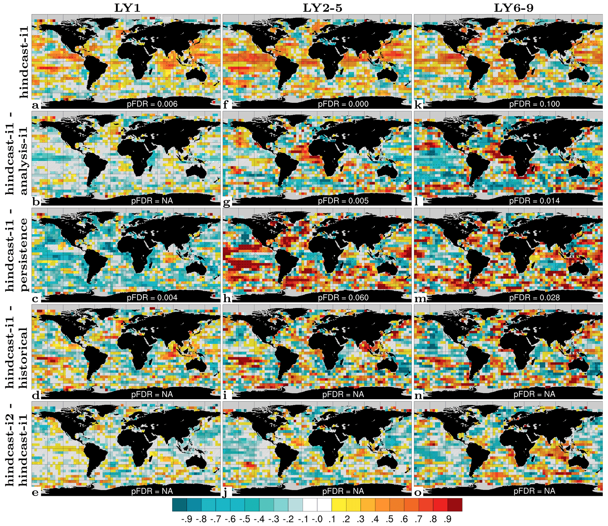
Figure 14Prediction skill for PP. ACC of hindcast-i1 (a), ΔACC of hindcast-i1 – analysis-i1 (b), ΔACC of hindcast-i1 – persistence (c), ΔACC of hindcast-i1 – historical (d) and ΔACC of hindcast-i2 – hindcast-i1 (e) for LY1. The middle and right columns show the same but for LY2–5 (f–j) and LY6–9 (k–o). Observations use GlobColour (Garnesson et al., 2019) with coverage for 1998–2018. Hatched areas are not locally significant; dotted areas are field significant.
Using satellite chlorophyll measurements for model evaluation is subject to caveats. For example, temporal data coverage is relatively short and the spatial data coverage at high latitudes is poor due to cloudiness. Following Yeager et al. (2018), we therefore also analysed the model's ability to hindcast its own analysis over the period 1960–2018 (Fig. 15). We will refer to this as the potential predictability*, using the asterisk to indicate that it differs from more conventional potential predictability estimates based on self-prediction that typically utilize a pre-industrial control simulation (e.g. Collins et al., 2006). The results become less patchy, and the total skill stays field significant for large parts of the global ocean until LY6–9. Removing the skill of historical again reveals that there are regions where the skill is improved by initialization, notably the subtropical gyres and the Nordic Seas (Fig. 15d, i, n). Note that subtracting negative historical ACCs leads to ΔACCs higher than the absolute ACCs of hindcast-i1 itself. Therefore, a large skill benefit from initialization does not necessarily translate into a societally useful absolute skill. We analysed time series of region-averaged PP between 1970–2018 in regions of high skill, namely the subtropical gyres of the Pacific, Atlantic and Indian oceans, as well as the Nordic Seas (not shown). The Nordic Seas are the only region with a strong positive correlation between hindcast-i1 and historical (r=0.5 and 0.6 for single year and four-year means, respectively), indicating that there is a large contribution of the external forcing to the predictive skill. There, the correlation between the hindcast-i1 and assim-i1 is close to 0.75 for all lead year ranges, indicating an improvement with respect to historical, with the largest difference for LY1. For the other regions, there is considerable agreement between the hindcast-i1 and the assim-i1 for LY1, with correlations exceeding 0.7. For the subtropical gyres in the Pacific and South Atlantic, the agreement between the hindcasts and the analysis extends to LY2–5, while the skill in the Indian and North Atlantic oceans drops beyond LY1.
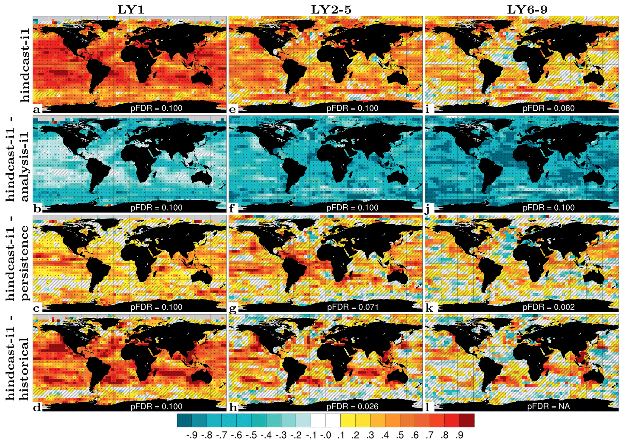
Figure 15Potential predictability* for PP. ACC of hindcast-i1 (a), ΔACC of hindcast-i1 – analysis-i1 (b), ΔACC of hindcast-i1 – persistence (c) and ΔACC of hindcast-i1 – historical (d) for LY1. The middle and right columns show the same but for LY2–5 (e–h) and LY6–9 (i–l). Synthetic observations constructed from the ensemble mean of the first 10 members of assim-i1 with coverage for 1960–2018. Hatched areas are not locally significant; dotted areas are field significant.
Despite the ambiguous results, the predictability of PP of a couple of years in the tropical/subtropical Pacific is in agreement with the results from perfect model experiments (Fransner et al., 2020) and Séférian et al. (2014), who found a predictability of 2–5 years when comparing with satellite-based PP in the same region. Also, Krumhardt et al. (2020) found a potential predictability of PP of a couple of years in tropical/subtropical regions when comparing to a reconstruction based on an ocean simulation forced with an atmospheric reanalysis. However, to remove the effect of external forcing, they performed a linear detrending. This partly removes the effect of climate change but not of other episodic external forcing such as volcanic eruptions. Frölicher et al. (2020) found a perfect model predictability of more than 10 years in some parts of the subtropical gyres in their perfect model study.
Studies have yet to report predictability of PP in high latitudes if compared to observational data. In these regions, the use of satellite observations is not reliable because of the lower data coverage and more variable chlorophyll-to-carbon ratio of phytoplankton (Frigstad et al., 2014). However, several recent perfect and potential predictability studies suggest that predictability of primary production in high latitudes is low or even non-existent on interannual-to-decadal timescales (Fransner et al., 2020; Frölicher et al., 2020; Krumhardt et al., 2020).
For CO2 fluxes (linearly detrended), a high total skill is found for all lead years but with initialization benefit limited to LY1 in the tropical Pacific, indicating that most skill stems from external forcing (Fig. S14 and text in Sect. S2). The modest benefit from initialization agrees with the findings of Lovenduski et al. (2019), who compared hindcasts of the CESM Decadal Prediction Large Ensemble (DPLE; Yeager et al., 2018) with the same observational dataset. However, other model systems (Li et al., 2016; Ilyina et al., 2020) and perfect model studies (Séférian et al., 2018; Fransner et al., 2020) have shown a predictability of unforced CO2 flux variability up to several years, particularly in the North Atlantic subpolar gyre, suggesting that there is room for improvement for the NorCPM1 decadal predictions.
3.2.4 Sea ice variability
Previous studies have found robust initialization benefits for sea ice prediction lasting for a couple of months (Guemas et al., 2016), with some re-emergence of skill during the second year (Day et al., 2014). While these studies reported strong seasonal dependencies, the evaluation here is limited to hindcasts initialized in November. We evaluate LY1 predictions of annual-mean sea ice concentration (SIC) against HadISST1 (Rayner et al., 2003) over the period 1960–2018 that includes historical observations as well as satellite estimates (Fig. 16). In the Arctic, the uninitialized predictions (historical) show externally forced skill in the Barents, Kara and Chukchi seas as well as the Canadian Archipelago (Fig. 16a). hindcast-i1 shows consistently higher ACCs than historical in these regions and additionally exhibits first-year skill in sub-Arctic regions, e.g. in the Bering and Greenland seas (Fig. 16b). hindcast-i2 benefits from a stronger constraint on the sea ice initial state compared to hindcast-i1, resulting in generally higher and more widespread skill (Fig. 16c). In the Antarctic, historical shows patches of both positive and negative ACC (Fig. 16d). There are nearly no regions where hindcast-i1 shows negative ACC, while regions with positive ACC are limited to the east Pacific sector of the Southern Ocean (Fig. 16e). hindcast-i2 shows even more positive skill, which extends into the Atlantic sector (Fig. 16f), but also some negative skill in the Pacific sector, albeit less negative than that in historical.
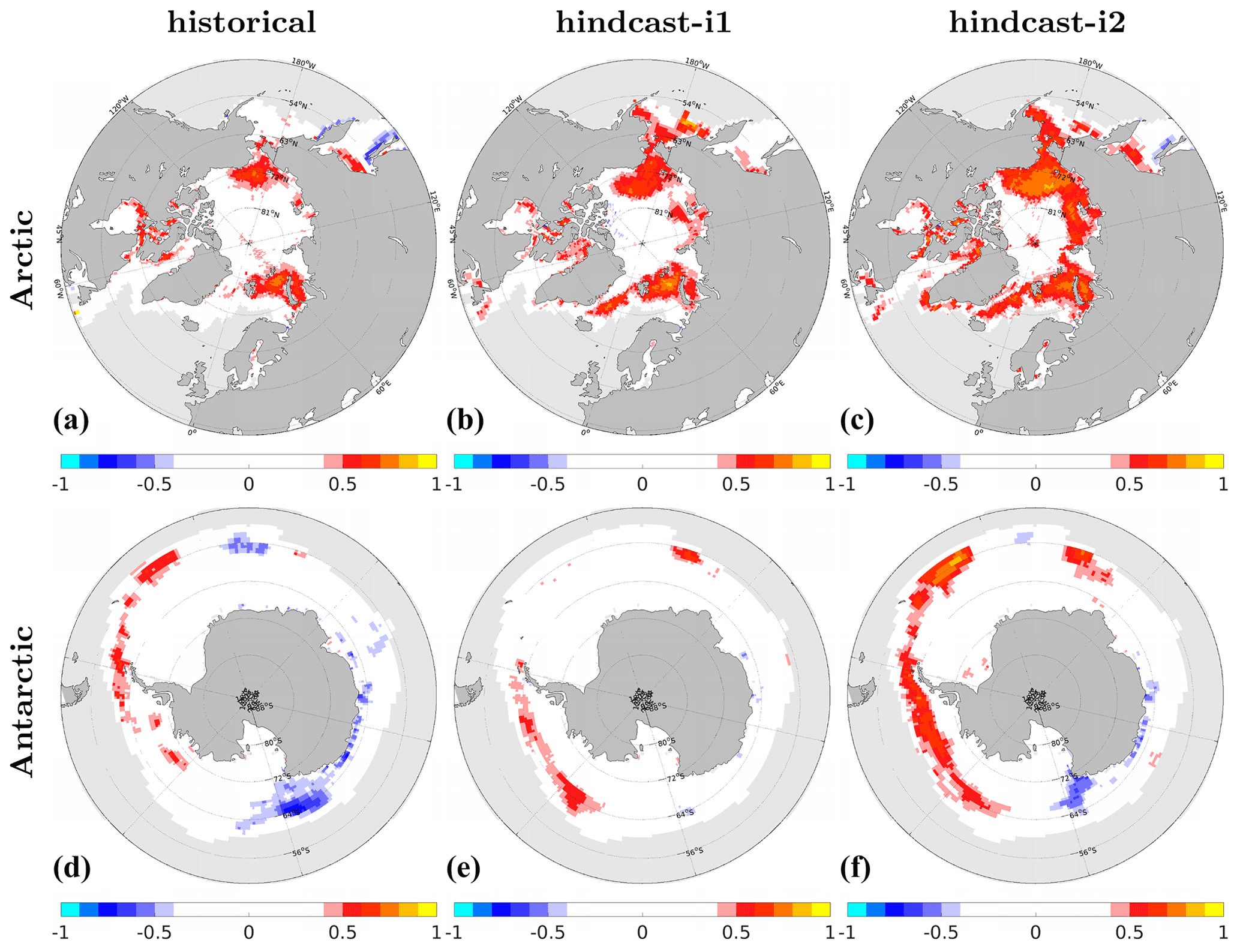
Figure 16ACC for sea ice concentration (SIC) for historical (a, d), hindcast-i1 (b, e) and hindcast-i2 (c, f) in the Arctic (a, b, c) and Antarctic (d, e, f) for LY1. Observations are from HadISST1 (Rayner et al., 2003) over the period 1960–2018. The data are interpolated to a regular grid.
We address seasonal dependence and temporal forecast limit of sea ice prediction by computing the ACC of total Arctic and Antarctic sea ice area as a function of lead month after November initialization (Fig. 17a, c). The Arctic ACC of persistence drops rapidly and both hindcast-i1 and hindcast-i2 show comparable or higher skill during the first winter and into spring. From early summer, the ACCs of hindcast-i1 remain close to zero. In contrast, hindcast-i2 shows some re-emergence of skill from the first autumn extending into the second year. Performing 3-month pre-averaging makes the skill re-emergence for hindcast-i2 and improvements over hindcast-i1, persistence and historical clearer (Fig. 17b, d). The uninitialized prediction from historical shows some skill during autumn and winter but no skill during summer. For the Antarctic, both uninitialized and initialized predictions perform inferior to persistence, with hindcast-i1 performing worst (Fig. 17c, d). Nevertheless, assim-i1 and assim-i2, which provide the initial conditions for hindcast-i1 and hindcast-i2, outperform persistence during most of the year, except in austral winter when persistence shows re-emerging skill. This suggests that model errors are skill limiting rather than imperfect initialization in that region.
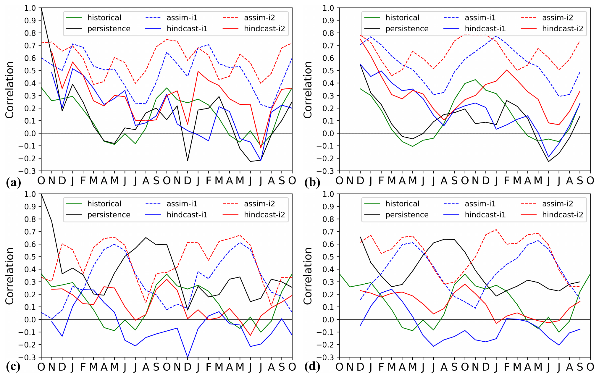
Figure 17ACC for Arctic (a, b) and Antarctic (c, d) total ice area as a function of lead month for monthly averages (a, c) and 3-month averages (b, d). The persistence forecast uses the observed October mean, while the hindcasts were initialized 1 November. Observations are from HadISST1 (Rayner et al., 2003) and limited to the satellite era (1979–2018).
Since regional sea ice variability is not necessarily in phase with total hemispheric sea ice area, we define a hemispherically integrated skill score for predicting local (i.e. grid-cell scale) sea ice conditions (Fig. 18). We first interpolate observation and model data to a common grid and then reduce the space and time dimensions to a vector that is used in the ACC computation. We apply square root grid-cell area weighting and only consider cells with non-zero temporal standard deviation. The squared score gives the fraction of predicted sea ice concentration variance. A theoretical score of one would imply perfect prediction in every location (note the score depends on the resolution of the common grid). In addition to monthly ACCs (Fig. 18a, c), we present 3-monthly ACCs (Fig. 18b, d) that are smoother. For the Arctic (Fig. 18a), the hindcast-i2 score reaches 0.4 during the first lead month, outperforming the sharply dropping persistence score (with 1-month e-folding scale) and remains significantly higher than the uninitialized historical score throughout winter and spring and marginally higher during the remainder of the two lead years. persistence shows a re-emergence of skill during summer and autumn that is present but weaker in hindcast-i2. hindcast-i1 shows a score below 0.3 for the first lead month and no initialization benefit after the first spring. Consistent with these differences in hindcast scores, assim-i2 features consistently higher scores than assim-i1. For the Antarctic (Fig. 18c), the initialized predictions do better than the uninitialized ones (with no or negative skill) but for the most part fall behind persistence. assim-i2 shows notably higher and more stable skill than assim-i1, explaining better performance of hindcast-i2 over hindcast-i1.
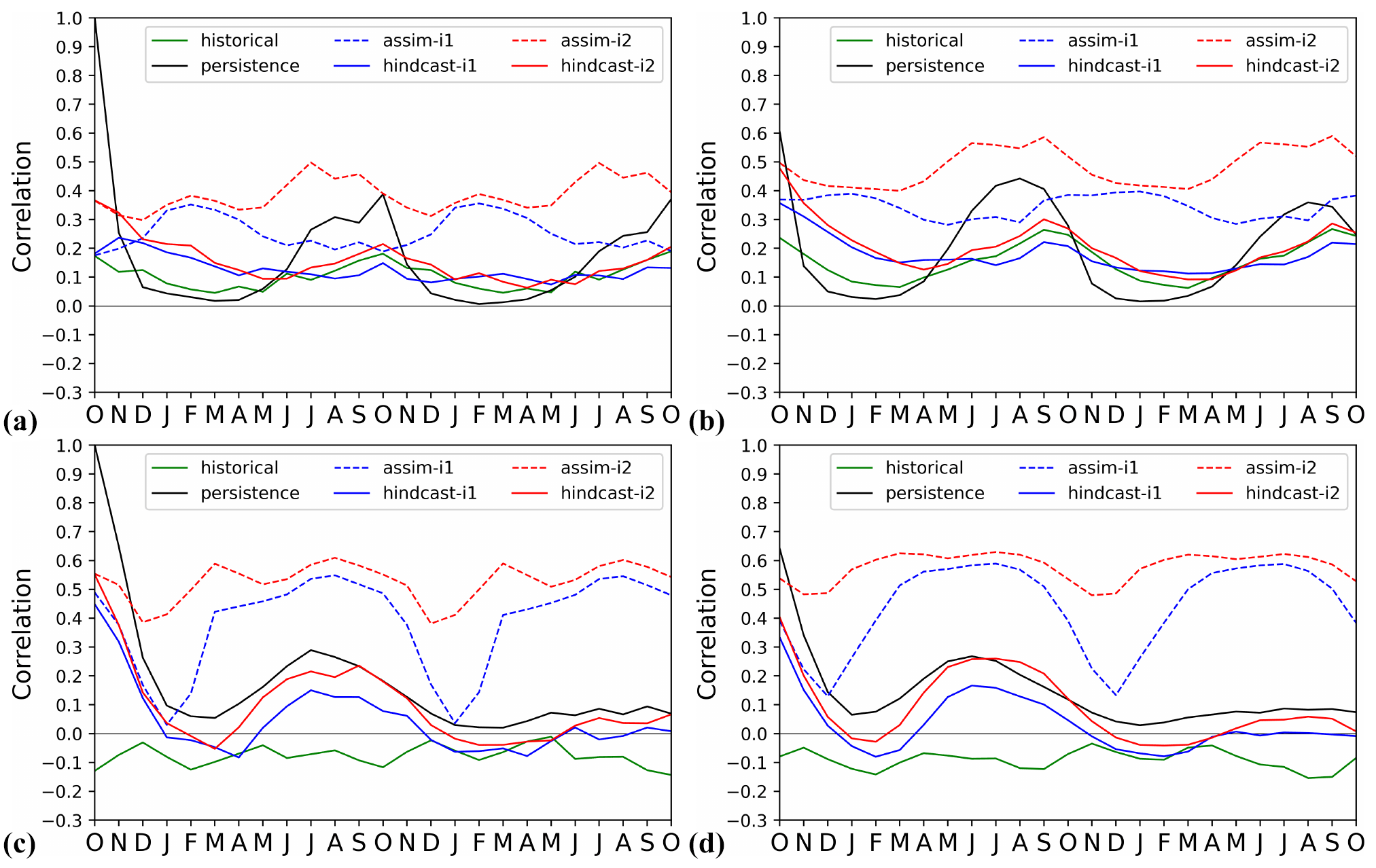
Figure 18Hemispheric correlation skill for Arctic (a, b) and Antarctic (c, d) ice area as a function of lead month for monthly averages (a, c) and 3-month averages (b, d). The data are first interpolated to a grid and correlations are then computed jointly over space and time, applying area weighting and only considering grid cells with non-zero temporal standard deviations. The persistence forecast uses the observed October mean, while the hindcasts were initialized 1 November. Observations are from HadISST1 (Rayner et al., 2003) and limited to the satellite era (1979–2018).
We have demonstrated initialization benefits for predicting sea ice up to two years ahead in NorCPM1, but can initialization improve prediction of decadal trends in Arctic sea ice decline? An analysis of Northern Hemisphere integrated sea ice volume (SIV) provides little evidence for that (Fig. S15). The initialized hindcasts have a tendency to simulate a flatter trend than the historical experiment over the last decade, which arguably can be interpreted as an improvement. Despite the lack of initialization benefit, the comparison between the two reanalysis products and their corresponding hindcasts is instructive and illustrates the importance of forecast drift correction. As mentioned in Sect. 3.1, the sea ice state update in assim-i2 overall reduces the simulated SIV to values closer to observations, whereas the climatology of assim-i1 remains unaffected. Once assimilation is stopped, the sea ice in hindcast-i2 grows back towards levels comparable to the no-assimilation historical experiment. As a result, the hindcast-i2 predictions all simulate strongly positive decadal SIV trends, whereas hindcast-i1 produces flat or negative trends more in line with observations. Adjusting for lead-dependent forecast drift largely eliminates differences in the decadal SIV trends between the two hindcast products.
3.2.5 Atmosphere variability
Transfer of skill from the ocean to the atmosphere and over land is key to societally relevant climate prediction. We assess the extent such transfer is realized in NorCPM1 from ACCs of SAT, PR, 500 hPa geopotential height (Z500) and sea level pressure (SLP).
For SAT, hindcast-i1 shows considerable first-year and multiyear hindcast skill that exceeds persistence skill over most land areas, except over central South America and parts of Africa and South Asia (Fig. 19a, c). The LY1 initialization benefit (Fig. 19d) is highest over the subpolar North Atlantic, extending from there over Scandinavia and western Siberia. Siberia is also the only region where hindcast-i2 consistently shows higher skill than hindcast-i1 (Fig. 19e). While the ΔACCs are not field significant, it is plausible that differences in sea ice initialization impact skill over adjacent land (Ringgaard et al., 2020). For LY1, the ΔACCs relative to historical (Fig. 19d) hint ENSO-related initialization benefits over low-latitude coastal regions as well as over northwest North America. For LY2–5 and LY6–9, the difference maps indicate little initialization benefit, implying that most multiyear SAT skill over land stems from the externally forced trend in NorCPM1. However, this result can be sensitive to the ΔACC metric (Fig. S18 and related discussion in Sect. 4).

Figure 19Prediction skill of 2 m temperature (SAT). ACC of hindcast-i1 (a), ΔACC of hindcast-i1 – analysis-i1 (b), ΔACC of hindcast-i1 – persistence (c), ΔACC of hindcast-i1 – historical (d) and ΔACC of hindcast-i2 – hindcast-i1 (e) for LY1. The middle and right columns show the same but for LY2–5 (f–j) and LY6–9 (k–o). Observations use HadCRUT4 (Morice et al., 2012) with coverage for 1950–2019. Hatched areas are not locally significant; dotted areas are field significant.
For PR, hindcast-i1 exhibits positive skill over most land regions for all lead ranges (Fig. 20a, f, k). For LY1 it is highest and field significant over the western tropical Pacific and Indonesian Archipelago (Fig. 20a). The LY1 skill difference to historical (Fig. 20d), a measure for the benefit from initialization, resembles the hindcast-i1 skill itself, suggesting only a small contribution from the externally forced trend to the first-year skill. For LY2–5 and LY6–9, the hindcast-i1 skill over the western tropical Pacific, Indonesian Archipelago and Australia is considerably reduced or disappears, whereas it is enhanced over north Africa, North America and northern Eurasia (Fig. 20f, k). It is plausible to assume that the bulk of the multiyear skill is driven by the externally forced changes in rainfall patterns and hydrological cycle (Dong and Sutton, 2015), which is evidently the case over north Africa where ΔACCs relative to historical are small or even negative (Fig. 20i, n). However, positive ΔACCs over western North America and northern Eurasia for all lead ranges suggest contributions from initialization. Most ΔACCs for precipitation are not field significant and we cannot preclude that they are a sampling artefact. This is in particular true for the hindcast-i2 and hindcast-i1 precipitation skill differences (Fig. 20e, j, o).
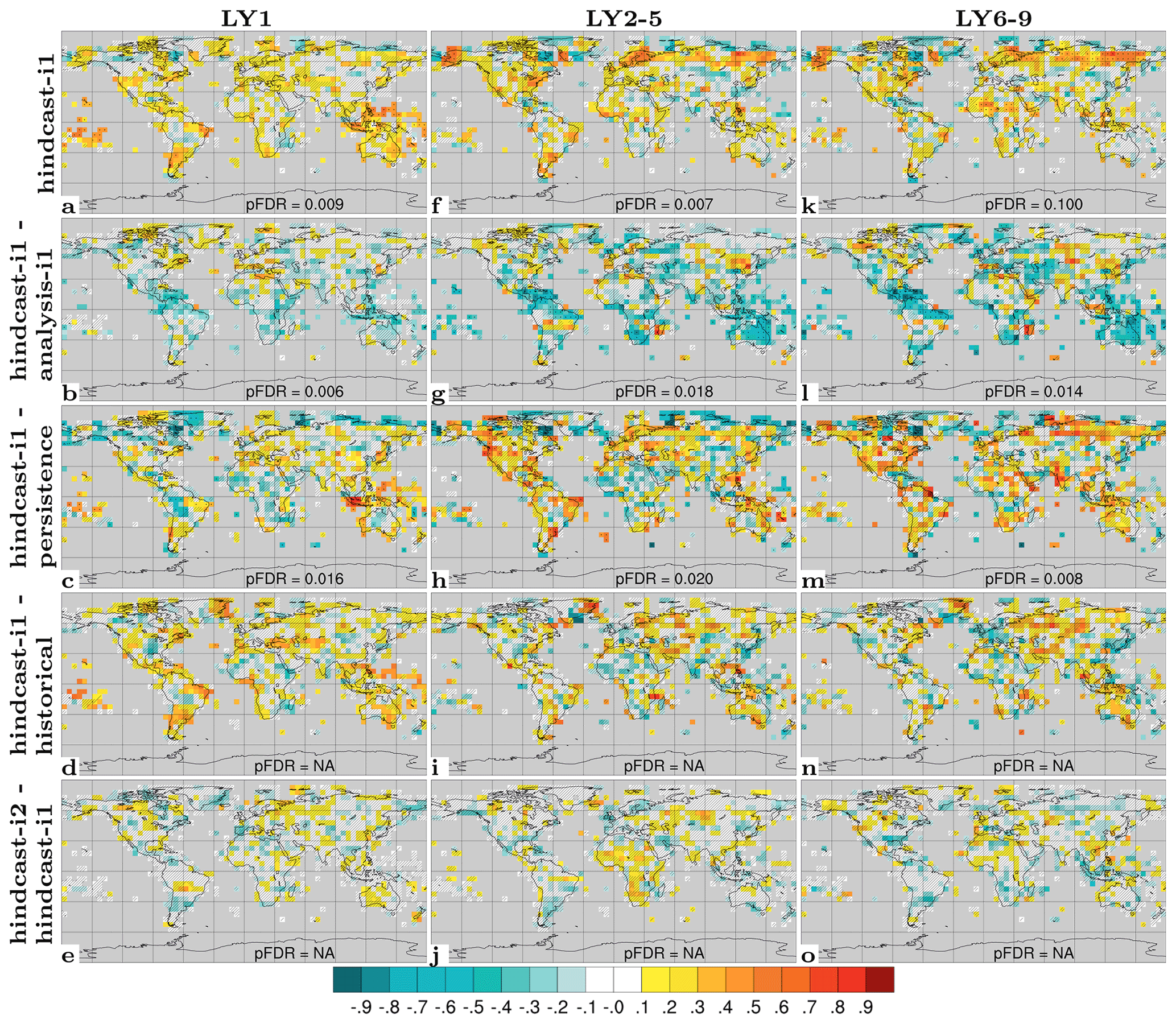
Figure 20Prediction skill of PR. ACC of hindcast-i1 (a), ΔACC of hindcast-i1 – analysis-i1 (b), ΔACC of hindcast-i1 – persistence (c), ΔACC of hindcast-i1 – historical (d) and ΔACC of hindcast-i2 – hindcast-i1 (e) for LY1. The middle and right columns show the same but for LY2–5 (f–j) and LY6–9 (k–o). Observations use CRU TS4.03 (Harris et al., 2020) with coverage for 1950–2018. Hatched areas are not locally significant; dotted areas are field significant.
Initialization benefits for predicting atmospheric circulation variability, as diagnosed from Z500 (Fig. S16) and SLP (Fig. S17), are most robust for LY1 owing to the influence of ENSO. For SLP, some multiyear initialization benefits are also present – albeit not field significant – over the extratropical Atlantic Ocean and Indian Ocean as well as the North American and Eurasian continents. The DA update of sea ice in hindcast-i2 slightly improves the multiyear skill in the Arctic, though the differences are small and not field significant.
3.2.6 Global skill evaluation
We globally summarize first-year and multiyear prediction skills by computing ACCs over time and space for the variables assessed in previous sections (Fig. 21). Skills are computed for LY1, LY2–5 and LY6–9 for the two analyses and hindcast products and benchmarked against the uninitialized historical predictions and persistence. The results are not particularly sensitive to grid-cell variance normalization and therefore similar to the globally averaged local (i.e. grid cell) ACC and also qualitatively similar to the mean-square skill score (not shown).
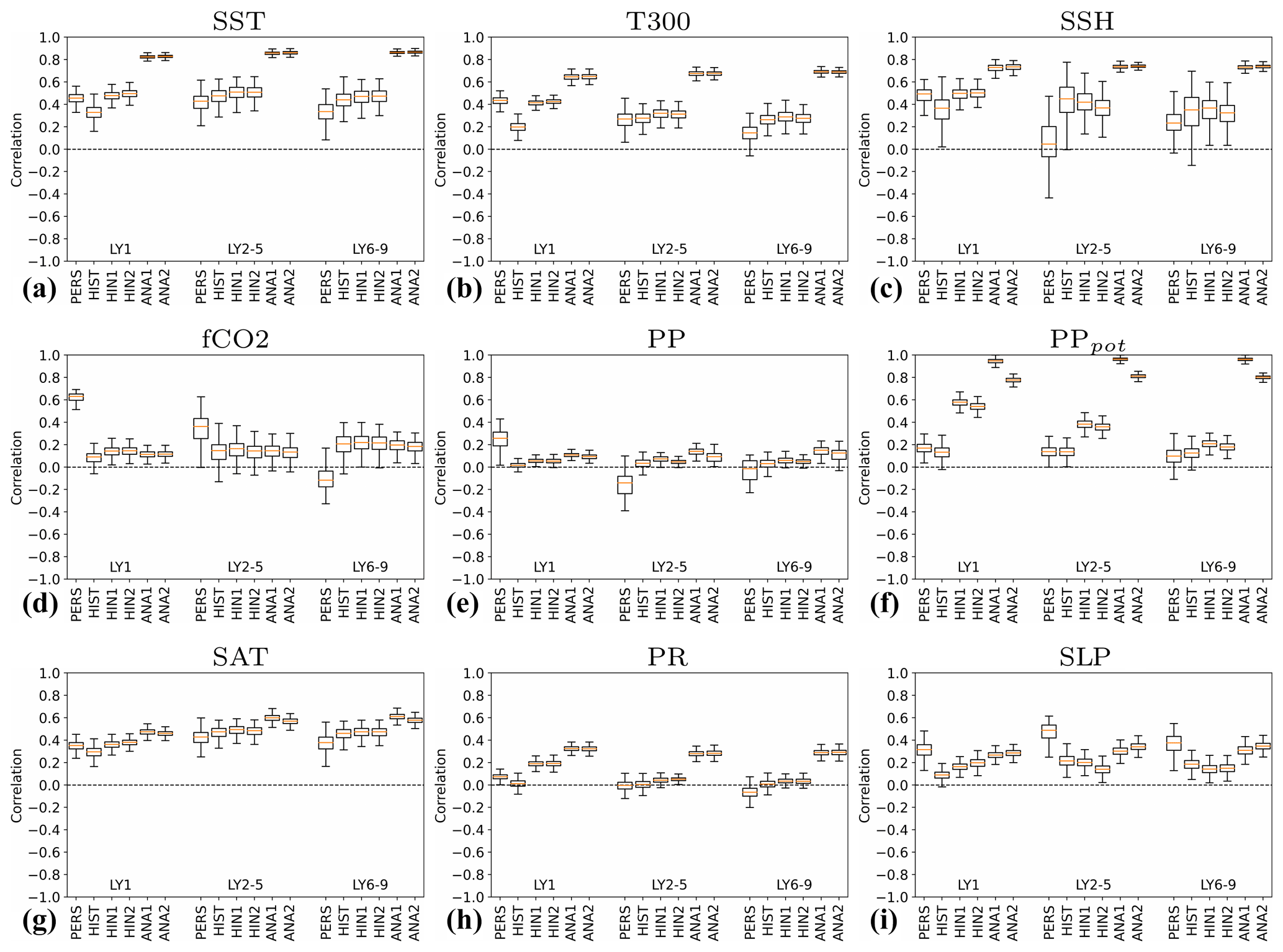
Figure 21 Global correlation skill for sea surface temperature (SST, a), 0–300 m temperature (T300, b), sea surface height (SSH, c), surface CO2 flux (fCO2, d), column-integrated primary production (PP, e, f), 2 m air temperature (SAT, g), land precipitation (PR, h) and sea level pressure (SLP, i). The ACCs are computed over time and space after weighting with the square root of the cell area. The box plots are constructed from 1000 bootstrap ACC realizations. Potential predictability* of PP (f) is referenced to assim-i1.
For SST (Fig. 21a), which is assimilated, the ACCs of assim-i1 and assim-i2 exceed 0.8 for all lead year ranges. After assimilation is discontinued, the values drop to 0.5 during the hindcasts. For LY1, this is still higher than and well separated from the 0.4 value of the historical experiment, suggesting statistically robust benefit from initialization for dynamical prediction with NorCPM1. Consistent with better first-year skill in ice-covered regions, hindcast-i2 performs slightly better than hindcast-i1, and both hindcast products exhibit marginally higher skill than persistence for LY1 (differences are not statistically significant). For LY2–5 and LY6–9, the ACCs of the two analyses and initialized hindcast products are very similar to or slightly higher than those for LY1. For multiyear prediction, the ACC of the historical experiment is on par with the initialized hindcast products, suggesting a major contribution from the externally forced trend and negligible initialization benefit. The fact that persistence scores lower than the uninitialized historical experiment reveals that the skill contribution from the externally forced trend is more than what could be expected from a linear anthropogenic climate trend. For T300 (Fig. 21b), the ACCs of the two analyses are 0.6–0.7, i.e. lower than for SST, presumably due to lower data coverage and higher observation error. Similar as for SST, a clear initialization benefit manifests for first-year prediction and only a hint of benefit for multiyear prediction. SSH (Fig. 21c) shows initialization benefit for first-year prediction but signs of detrimental initialization impact for multiyear prediction. The ACC estimates for SSH are more uncertain than for T300, partly owing to the shorter evaluation period.
Surface CO2 flux (Fig. 21d) and primary production (Fig. 21e) are poorly constrained by the assimilation with the two analyses exhibiting ACCs of 0.2 and below. It is therefore unsurprising that the initialized hindcasts are not skilful and at best show marginal initialization benefit over likewise unskilful uninitialized predictions of historical. However, Ilyina et al. (2020) found a predictability of the global air–sea CO2 fluxes of up to 6 years when combining the members of the two hindcast sets, suggesting considerable sensitivity to the chosen biogeochemistry skill metric, spatial averaging, evaluation period and ensemble size. In contrast to the hindcasts, the persistence skill for CO2 flux exceeds 0.6 for LY1 and 0.3 for LY2–5, and for PP is close to 0.3 for LY1. When using assim-i1 as observational truth for primary production (Fig. 21f), the system suggests initialization benefit for all lead years with hindcasts reaching ACCs close to 0.6 for LY1. Inherent issues in the marine ecosystem parameterization to represent realistic variability (Tjiputra et al., 2007; Gharamti et al., 2017) in combination with observational uncertainties are likely causing this discrepancy.
Assimilation in NorCPM1 updates the ocean and sea ice state but does not directly constrain the atmospheric and land states. Nevertheless, the assimilation can improve their prediction to the extent that SST and sea ice control the atmospheric state. The ACCs for SAT (Fig. 21g) resemble those for SST, but are lower, in particular for the two analyses. Land precipitation (PR) exhibits ACCs of 0.4 independent of lead year range for the two analyses, and 0.2 for the hindcasts for LY1, suggesting some success in initializing ENSO. Contrary to SAT, the historical experiment and persistence both exhibit zero skill for PR, both for annual means and multiyear means, despite anthropogenic spin-up of the hydrological cycle and other external influences. SLP (Fig. 21i) behaves differently in that the global ACCs of persistence, ranging between 0.3 and 0.5, are consistently higher than those of NorCPM1. Thus, the external forcing seems to have a significant influence on the observed SLP variability, but NorCPM1 fails to capture it. For LY1, the ACCs of the initialized hindcasts are slightly higher than those of the historical experiment, again suggesting skilful initialization of ENSO.
We finally evaluate how well the system constrains the temporal evolution of global means (Fig. 22). Especially in the context of climate change attribution, it is of interest whether DA leads to improved representation of global surface warming, global sea level change and strength of the global hydrological cycle. The initialized hindcasts outperform persistence and historical for SST and SAT for LY1. Beyond that, the results show little evidence of initialization benefit, except a marginal improvement of multiyear mean prediction for the oceanic CO2 flux and a sizable potential predictability* benefit for PP. While the initialized hindcasts performed as well as or better than historical for globally averaged skill of local SST, T300 and SAT (Fig. 21a, b, g), hindcast-i1 and hindcast-i2 show slightly poorer multiyear skill than historical in their global means (Fig. 22a, b, g). Except for SST, the reanalyses mostly outperform both persistence and historical but not as clearly as for the globally averaged skill. Interestingly the benefit from DA is considerably larger for global precipitation than for global-mean SST, possibly indicating a strong control of well constrained tropical – likely ENSO-related – SST variability on large-scale precipitation. DA does not improve the match with the 16-year short observational record of global sea level. Why exactly the globally averaged grid-cell skills (Fig. 21) show more benefit from DA than the skills of the global means (Fig. 22) is something that warrants further investigation.
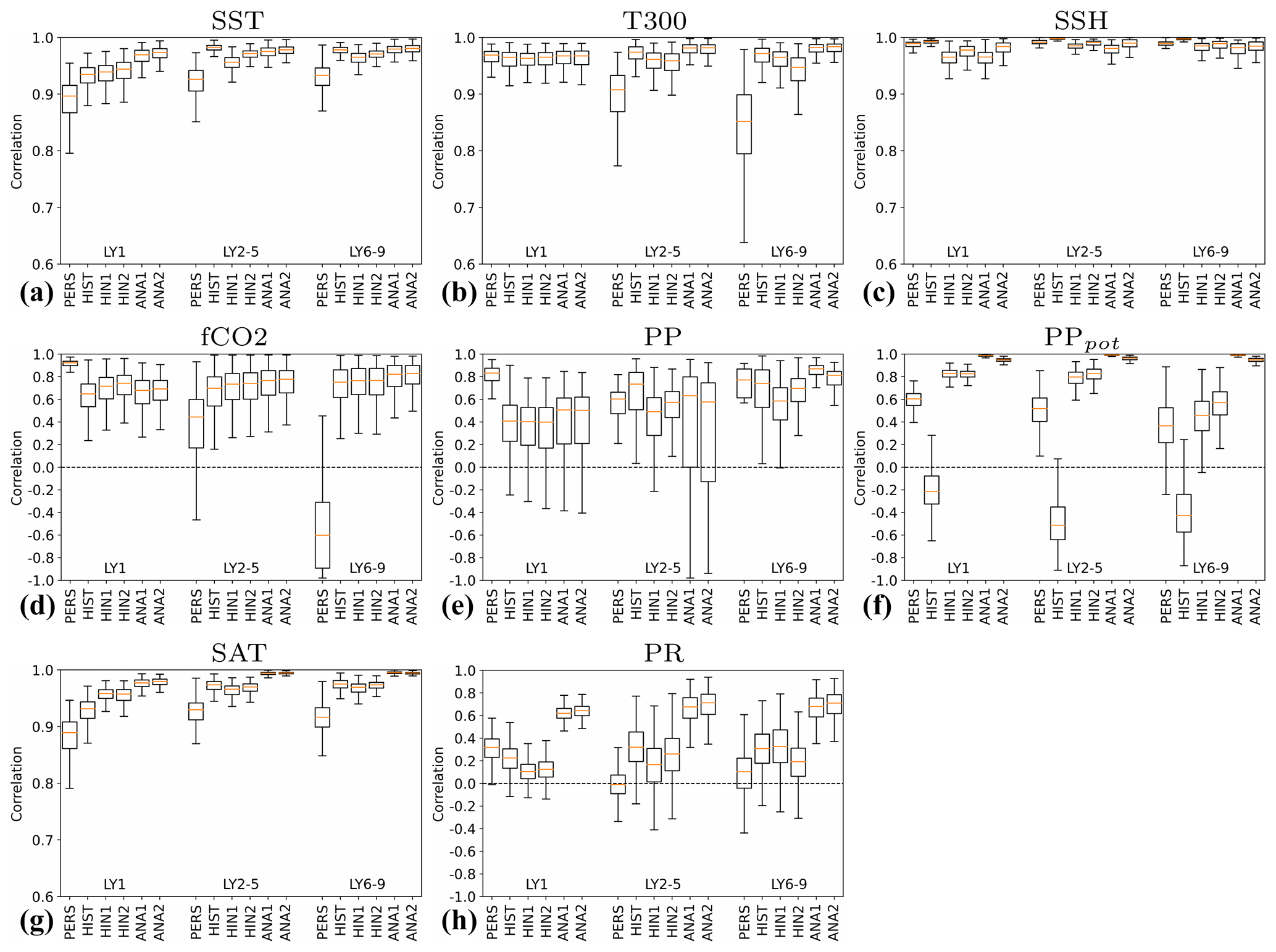
Figure 22Correlation skill for global means of sea surface temperature (SST, a), 0–300 m temperature (T300, b), sea surface height (SSH, c), surface CO2 flux (fCO2, d), column-integrated primary production (PP, e, f), 2 m air temperature (SAT, g) and land precipitation (PR, h). The box plots are constructed from 1000 bootstrap realizations of the correlations. Potential predictability* of PP (f) uses assim-i1 instead of real observations. The plotted correlation range varies for different variables.
Evaluating interannual-to-multiyear variability in NorCPM1 simulations with and without DA against observations, we found measurable initialization benefits – particularly for first-year prediction – and only few signs of detrimental effects from DA. In this section, we will further discuss the findings, related caveats and potential improvements.
The anomaly assimilation scheme of NorCPM1 currently updates only the ocean and sea ice components, and the atmosphere and land components are only constrained to the extent that they are affected by the surface conditions. Utilizing atmospheric observations and better constraining the atmospheric circulation variability has potential to improve the ocean and sea ice initialization by producing surface fluxes that are more consistent with the SST and SIC anomalies during the assimilation phase. Constraining the atmospheric circulation will also improve atmosphere and land initialization, beneficial for subseasonal-to-seasonal prediction. The success of utilizing initial conditions from forced ocean–sea ice simulations (Yeager et al., 2018) demonstrates the potential in constraining surface fluxes over ocean and sea ice for initializing multiyear climate predictions. Performing EnKF ocean–sea ice assimilation in addition to constraining the atmospheric variability is expected to further improve the predictions (Polkova et al., 2019). Utilization of atmospheric observations in NorCPM's initialization is a work in progress. A unified EnKF-based assimilation scheme covering all ESM component would be desirable but is subject to numerous technical and scientific challenges. As an intermediate solution, we are exploring atmospheric nudging in combination with EnKF-based ocean–sea ice assimilation in NorCPM, a strategy that has been successfully applied in the Max Plank Institute Mittelfristige Klimaprognose (MPI-MiKlip) system (Polkova et al., 2019). We will take advantage of the availability of multiple simulation members of the reanalysis products like ERA5 (Hersbach et al., 2020) and CERA-20C (Laloyaux et al., 2018) and nudge the members of the NorCPM analysis to individual members of the reanalysis products to provide a representation of atmospheric observational uncertainties and help generate ensemble spread in the ocean state. We will complement the atmospheric nudging with the leading average cross-covariance technique that has been shown to further improve ocean initialization by performing a one-way (from atmosphere to ocean) strongly coupled data assimilation (Lu et al., 2015).
NorCPM1 shows overall high multiyear prediction skill from external forcing, with a modest and regionally limited increase in skill from improving the initial conditions via DA. A caveat with using ACC differences for detecting initialization benefit is that if the absolute ACCs are large, the ACC differences become difficult to robustly detect. Smith et al. (2019) proposed a more robust quantification method for initialization benefit, where the forced signal of the model is regressed out of both the model and observation data and ACCs are computed from the residuals (the result is scaled to account for the smaller variance of the residuals; see Sect. S2 for more details). Figure S18 compares both methods, with the residual ACCs showing clear initialization benefit for SAT over land regions where ΔACCs are statistically indistinguishable from zero. Like in Yeager et al. (2018), we use ΔACCs in this study to systematically compare against multiple benchmarks. The use of residual ACCs should, however, be of interest for future work, especially for assessing the impact of DA developments on forecast skill.
While the focus of this study leans towards DA innovations, future skill improvement clearly depends also on improving the ESM component of NorCPM. The dynamical model representation has been demonstrated key to skilful climate prediction (Athanasiadis et al., 2020; Yeager et al., 2018) and recent studies revealed a larger role of external forcing than previously thought (Borchert et al., 2021; Klavans et al., 2021; Liguori et al., 2020). The skill benefit from DA-assisted initialization does not only relate to synchronization of internal climate variability, but also to correcting the externally forced climate signal at forecast initialization time – which is subject model and forcing errors. We nevertheless expect a continuous need for, and benefit from, improving NorCPM's assimilation, along with improving its ESM component. We have seen from weather and seasonal forecasting how improvements in both models and methods to assimilate observations (as well as observations and computing power) have continued to lead to enhanced prediction skill (Bauer et al., 2015). Work has started to upgrade NorCPM's ESM component to NorESM2-MM (Seland et al., 2020) – featuring improved physical process parameterizations, a higher atmospheric resolution, a more realistic AMOC and overall reduced climate biases compared to NorESM1 – and results of this effort will be documented in future publications. We envision that the climate prediction evaluation and DA can increasingly inform the development of NorESM, which traditionally focused on long-term climate projections. There is growing evidence that current generation climate models systematically underestimate the influence of SST variations and external forcing variability on extratropical atmospheric variability, particularly related to the North Atlantic Oscillation (e.g. Scaife and Smith, 2018; Athanasiadis et al., 2020). While post-processing methods relying on large ensembles have been proposed to mitigate this shortcoming (Smith et al., 2020), improving this aspect in the next model generation should be a key priority for the prediction community.
The significance testing used in this study (Appendix B) does not account for observational error. Nowadays, observational reanalyses routinely provide ensemble products that span observational uncertainty. While they are beyond the scope of this study, future skill evaluations should explore ways of utilizing this ensemble information in local and field significance testing. The addition of observational uncertainty should generally lower the p values, leading to stricter testing.
The ACC, our primary metric for quantifying skill in this study, is sensitive to random correlation that can occur over the evaluation period as it does not penalize for amplitude errors. The mean-square skill score (MSSS), that penalizes amplitude errors, can be used as an alternative, potentially more robust metric (Goddard et al., 2013, and Sect. S2). As we found the MSSS results (Fig. S19) comparable to the ACC results (Fig. S10), we decided to use ACC to facilitate comparison with previous works (e.g. Yeager et al., 2018) and because amplitude errors stemming from the model underestimating the forced climate signal can to some extent be corrected posteriori (Smith et al., 2019; Smith et al., 2020). Our skill evaluation based on annual means does not address seasonal effects. Separately evaluating the skill for individual seasons may help us better understand the origins of skill and utility for society.
The Norwegian Climate Prediction Model version 1 (NorCPM1) is a new climate prediction system that has contributed with model output to the Decadal Climate Prediction Project as part of the Coupled Model Intercomparison Project phase 6 (CMIP6 DCPP). NorCPM1 combines the Norwegian Earth System Model version 1 (NorESM1) with an ensemble Kalman filter (EnKF) anomaly assimilation of sea surface temperature and hydrographic profile observations. This paper provides a description and evaluation of NorCPM1.
Compared to other dynamical climate prediction systems, NorCPM1 distinguishes itself by its EnKF anomaly assimilation that performs cross-component ocean-to-sea-ice updates and is optimized for an ocean vertical density coordinate. The EnKF scheme makes optimal use of the observations by also updating unobserved variables using state-dependent relations from the model's simulation ensemble. The use of these relations further minimizes shock by ensuring that all variables are updated consistently, to the extent the system behaves linearly. Through performing EnKF anomaly assimilation and accounting for measurement and representation errors in the observations, NorCPM1 aims at synchronizing internal variability in a targeted and gentle manner to provide a reliable system (i.e. where the ensemble spread reflects the true internal variability error) that is mostly free of detrimental prediction shock. While on a grid scale this allows certain mismatch between model and observations, our evaluation of the assimilation experiments shows that the approach accurately synchronizes the large-scale variability modes (such as ENSO, Pacific Decadal Oscillation (PDO) and SPG strength) that are likely to carry multiyear predictability.
The paper assessed the performance of the ESM component of the prediction system. Upgrades of the external forcings from CMIP5 to CMIP6 and minor code changes have only a minor impact on the model's climate representation relative to the original NorESM1, which contributed to CMIP5. Spatial biases in key climate variables have mostly remained the same, as has the global climate response to external forcings. The conditional bias is hence largely unaltered relative to previous NorCPM configurations. Noteworthy biases are a 50 % too-strong Atlantic meridional overturning circulation, excessive Arctic sea ice with cold adjacent continents, warm surface biases in the subpolar North Atlantic and Southern Ocean that are mirrored by cold biases at lower latitudes. In turn, the model's ENSO characteristics and its historical global warming compare favourably to observations.
The paper assessed the performance of the assimilation capability with two 30-member climate reanalyses products that have been contributed to CMIP6 DCPP. Both assimilate SST and -profile observations but differ in their treatment of sea ice and reference period used to construct anomalies. The anomaly assimilation of NorCPM1 does not show any detrimental effects on the climatology and generally reduces the RMSE of both observed and unobserved state variables (unobserved means not part of observation types that are assimilated) in the assimilation experiments relative to the historical experiment without assimilation. The application of cross-component anomaly assimilation reduces a positive bias in Arctic sea ice thickness and improves synchronization of sea ice variability and variability of other climate variables, such as Southern Ocean sea surface height.
A challenge unique to anomaly assimilation is how to best construct the anomalies. The choice of reference period has limited impact on their correlation scores with observations, but it has significant impact on mean and long-term trends, e.g. in Atlantic meridional overturning circulation strength and meridional ocean heat transport. Future NorCPM development efforts will explore more sophisticated ways of designing climate anomalies, e.g. following Chikamoto et al. (2019), addressing important issues such as conditional bias and separation of internal variability versus externally forced signals in observations.
The assimilation shows limited success in synchronizing variability in ocean biogeochemistry variables like net primary production or air–sea CO2 flux. This result contrasts findings of a perfect model study (Fransner et al., 2020) with the ESM component of NorCPM1 that suggests strong control of the physical state on interannual ocean biogeochemistry variability. Imperfect synchronization of physical variability, short evaluation periods, errors in observations and errors in the model representation of ocean biogeochemistry and its interaction with physical processes can contribute to this discrepancy.
The paper assessed the performance of the system to produce first-year and multiyear climate predictions. We found robust initialization benefits for first-year prediction across a range of climate variables that at least partly are related to skilful synchronization of ENSO variability. Predictability of sea ice extends into the second year in the hindcast product initialized from a reanalysis that more strongly constrains the sea ice state.
While the externally forced trend leads to significant multiyear prediction skill, our evaluation provides limited evidence for robust initialization benefits on multiyear timescales but also little indication for detrimental effects from initialization. Multiyear initialization benefit is mainly confined to SPNA in NorCPM1, where it largely offsets negative skill in uninitialized predictions and leads to modest absolute skill that is significantly lower than the skill from non-dynamical prediction such as persistence forecast. After removing the forced signal, the initialization benefit for SPNA translates into robust benefit for temperature over adjacent land. The comparison of two differently initialized hindcast products reveals a high sensitivity of the AMOC to the details of the initialization approach with considerable impact on SPNA temperatures, such as shift in mean state and long-term trend and hindcast drift behaviour. Notwithstanding that both products struggle predicting the circulation evolution, it indicates the potential for improving SPNA temperature predictions by improving initialization of hydrographic anomalies that condition the evolution of the large-scale ocean circulation. To realize the full potential, however, would require a model representation of the circulation with realistic mean state, variability and sensitivity to external forcing, aspects we will prioritize in further NorCPM development. Lead-dependent drift correction removes much of the differences between the two products (including a strong forecast drift in sea ice thickness present in one of the products) and therefore also has merits for anomaly-initialized predictions, in particular if model output is intended as input for climate impact studies.
The initialization of the physical model states does not robustly benefit ocean biogeochemistry predictions in NorCPM1. This is unsurprising given the aforementioned poor skill of the reanalyses used for hindcast initialization. Thus, improving and understanding the lack of skill in the reanalyses is paramount to improving NorCPM's ocean biogeochemistry capability.
We found robust transfer of initialization skill benefit to atmosphere and land for first-year prediction. As current climate models tend to underestimate atmospheric signal-to-noise ratios, more hindcast simulation members are expected to increase first-year skill and enable detection of multiyear signals (Scaife and Smith, 2018; Smith et al., 2020).
In summary, we found demonstrable benefits from initialization for climate prediction with NorCPM1. The initialization is virtually free of detrimental effects. At this stage, NorCPM1 primarily serves as a research tool. Based on the forecast quality evaluation presented in this paper, further development is needed to reach multiyear prediction skill at a societally useful level that makes the system more fit for operational use. To this end, the evaluation in this paper will serve as a benchmark for further NorCPM development, such as upgrades to the ESM component and refinements to the assimilation approach with extension to all model components. Deficiencies of NorCPM1 skill identified here will guide future research and model development. The system has demonstrated promising seasonal prediction capabilities (Wang et al., 2019; Kimmritz et al., 2019) and may already contribute to skilful multiyear climate prediction with societal application in a multi-model framework (Smith et al., 2020).
There are multiple ways to initialize hindcasts, such as initialization from existing reanalysis products produced with an independent system (e.g. Chikamoto et al., 2019) or initialization of the ocean component by running it uncoupled, forced with an atmospheric reanalysis product (Yeager et al., 2018). In NorCPM1, the hindcasts are initialized from a reanalysis produced with the same ESM that assimilates ocean observations with the Ensemble Kalman filter (EnKF; Evensen, 2003). The advantage of using the same ESM is that it avoids initialization adjustment that occurs when changing the model. The EnKF is an advanced flow-dependent data assimilation method where the multivariate corrections are based on a set of observations, their uncertainty and the ensemble of model realization produced by a Monte Carlo integration from the previous analysis step. Counillon et al. (2016) showed that the upper ocean heat content in the equatorial and North Pacific, the North Atlantic subpolar gyre region and the Nordic Seas can be well constrained by assimilating SST anomalies with the EnKF. In particular, the vertical covariance shows a pronounced seasonal and decadal variability that highlights the benefit of flow-dependent data assimilation. In NorCPM1, covariances in the ocean are formulated in isopycnal coordinates (the native vertical coordinate of the ocean model), which allows for deeper influence of the assimilated surface observations than when formulating them in standard depth coordinate (Counillon et al., 2016).
Up to now, climate prediction systems have predominantly assimilated data independently in their respective components, an approach referred to as weakly coupled data assimilation (WCDA; Penny and Hamill, 2017). The other model components adjust to these individual changes dynamically in between the assimilation cycles. Allowing the assimilation to update across model components is expected to outperform WCDA because it would enhance dynamical consistency of the initial condition and expand the influence of the observations across its own component (strongly coupled data assimilation, SCDA; Penny and Hamill, 2017; Penny et al., 2019). The climate system includes complex, coupled phenomena over wide, separated spatial and temporal scales of the Earth system components (atmosphere, ocean, land surface, cryosphere). DA procedures, on the other hand, are mostly designed to deal with a single dominant scale of motion or under the assumption of weak coupling (Laloyaux et al., 2016; Sun et al., 2020). Joint OSI-SCDA of ocean and sea ice has been successful with flow-dependent DA methods such as the EnKF. The scale separation between ocean and sea ice is not as pronounced as between ocean and atmosphere. The application of flow-dependent covariance can handle well the anisotropy and sign reversal of the covariance at the sea ice front (Lisæter et al., 2003; Sakov et al., 2012) and the update of the multi-category sea ice state (Massonnet et al., 2015; Kimmritz et al., 2018). Application of the methods has since also been tested successfully in a fully coupled ESM (Kimmritz et al., 2018) and used for seasonal prediction of Arctic sea ice (Kimmritz et al., 2019). A full SCDA of the ESM is a more challenging task because of the separation of spatial and temporal scales among atmosphere and ocean. There have been many advances both theoretically (Lu et al., 2015; Smith et al., 2015; Tardif et al., 2015; Sluka et al., 2016; Penny and Hamill, 2017) and on application, e.g. the CERA reanalysis (Laloyaux et al., 2016) but no system is yet at the stage of achieving a full SCDA. For interannual-to-decadal timescale, the largest part of climate predictability resides in the ocean and sea ice (e.g. Mariotti et al., 2018). Making use of the rich atmospheric observation network will be explored in future NorCPM versions as it can further improve the initialization of the slow modes of variability in the ocean where observations are sparse and generally enhance the consistency of the system.
Climate models have strong biases that are in some places larger than the internal variability (Richter et al., 2014). There are two common strategies in the climate prediction communities to handle bias: full-field assimilation requiring a subsequent post-processing to account for the model adjustment back to its own attractor or anomaly assimilation where the observed anomaly (calculated relative to a reference climatology) are imposed on a biased model climatology (Weber et al., 2015). Both methods have their advantages and disadvantages. NorCPM1 uses anomaly assimilation because full-field assimilation is problematic with ensemble DA (Dee, 2005): As models are attracted to their biased climatological states, the model bias in the observed variables is propagated to the non-observed variables by the multivariate covariance matrix, which leads to a slow degradation of the system through the consecutive assimilation cycle. A challenge when defining a climatological reference is to ensure that the climatological reference is accurate and representative of the same variability between the model and data. Estimating an accurate climatology for observations becomes problematic in regions where observations are very sparse, limiting the possible span of a reliable climatological period. Furthermore, while it is usually possible for the model to nullify the internal variability by averaging different ensemble members starting from different initial conditions, there is only a single realization of the truth, and one must ensure that the climatological period of the observation is long enough to cancel out internal variability. Finally, it should be added that anomaly assimilation only addresses climatological biases and conditional biases such as in the variability and in the forced trends.
An emerging number of climate prediction models include ocean biogeochemistry (e.g. Séférian et al., 2014; Li et al., 2016; Lovenduski et al., 2019; Park et al., 2019). Due to technical challenges with implementing ocean biogeochemistry in DA systems related to data sparsity and the non-Gaussian behaviour of many biogeochemical tracers, assimilation of biogeochemical observations is commonly not applied in these models (e.g. Park et al., 2019). Instead, the ocean biogeochemistry is treated passively. This has been shown to constrain the biogeochemical variability relatively well (Séférian et al., 2014; Li et al., 2019; Park et al., 2019). There are, however, problems related to the update of physics that introduces artificial mixing between surface and deep waters, leading to excessive surface nutrient concentrations and primary production, especially in the tropics (While et al., 2010; Park et al., 2018). Skilful near-term predictions of 4–7 years of air–sea CO2 exchange (Li et al., 2016, 2019), a couple of years for chlorophyll (Park et al., 2019) and 2–5 years for net primary production (NPP, Séférian et al., 2014) have been achieved by this passive initialization of ocean biogeochemistry. Fransner et al. (2020) showed, in a perfect model framework, that the initial state of ocean biogeochemistry has little impact on the prediction skill beyond LY1, and their work suggested that assimilation of biogeochemical tracers would only give a marginal improvement in the predictive skill of ocean biogeochemistry.
Following Goddard et al. (2013), we use the anomaly correlation coefficient (ACC) for assessing hindcast and reanalysis performance. We use ΔACC score differences for comparing our reanalysis and hindcast products and for benchmarking against uninitialized predictions and persistence forecast. As in Goddard et al. (2013), we consider lead year 1 (LY1), lead years 2–5 (LY2–5) and lead years 6–9 (LY6–9) forecast ranges using multiyear averages. For example, if a hindcast is initialized in October 1960, then LY1 corresponds to the average of 1961, i.e. the following calendar year.
If the temporal coverage of the observations is shorter than that of the model output, we maximize the use of observations in the ACC computation. For example, if the observations start in 1993 then the ACC computation for LY6–9 will use hindcasts starting at the end of 1983 and later. Consequently, the start dates used in the ACC computation may differ for the different forecast ranges, while the evaluation period is fixed except in the persistence forecast. The LY1 persistence forecast uses the observational average of the previous year, while the LY2–5 and LY6–9 persistence forecasts use the average over the four previous years. This is done because we found the effect of temporal filtering to outweigh the shift towards older observations, resulting in persistence skills consistently higher than if using the last month or last year instead.
Prior to the ACC computation, we interpolate model and observational data to a common, regular grid if not stated otherwise. We do not remove the linear trend or other estimates of the forced response, except when evaluating surface carbon flux. When comparing ACCs of hindcasts (which comprise 10 simulation members) with uninitialized predictions, we only use the first 10 members of historical because we want to isolate the benefit of initialization without confounding it with the effect of ensemble size on the accuracy of the externally forced trend estimate.
We test local and field significance of skill scores and score differences following Yeager et al. (2018). We consider a score locally significant if the associated p value (i.e. probability for producing a random score equal to or higher than the score tested) is below αlocal:=0.1 (i.e. 90 % confidence). Regions that fail the local significance test are marked with slash/on the skill score maps (e.g. Fig. 7). We derive the p values by means of resampling the original data that are interpolated to the common grid. For each obtained skill score we construct 4000 bootstrapped scores that capture random uncertainty stemming from temporal sampling and from having a limited ensemble size. Using the moving block bootstrapping technique, we resample the data (pairwise model–observation sampling with replacement) in 5-year blocks that may start in any year but not in the last 4 years to account for temporal autocorrelation. The blocks are concatenated, and the last block is truncated such that the bootstrapped time series has the same length as the original series. Additionally, we resample (with replacement) the ensemble members used in the computation of the ensemble means. While the combination of members varies between different bootstrapped time series, we keep it fixed within each series. We test significance for both positive and negative scores. Following Goddard et al. (2013), we estimate the p value for a particular skill score as the fraction of bootstrapped scores with opposite sign of that of the score tested (e.g. if the original score is positive and 200 out of the 4000 bootstrapped scores are negative, then we determine p as .05). The rationale is to utilize the spread information from the bootstrapped distribution to calculate the probability for obtaining a score equal to or higher than the score tested, under the null hypothesis that the true score is zero. We verified the bootstrap estimation of p values on a large set of artificially constructed series with known true correlation and found good agreement with Monte Carlo estimated p values, with r(pbootstrap, pMonteCarlo)>0.95.
Local significance information has particular utility if considering a single location of interest and if the choice of this location is not informed by the spatial score distribution. Explorative analyses, however, often simultaneously consider multiple locations of interest and make the selection of locations dependent on the spatial score distribution as they tend to focus on regions with the most extreme scores. In such cases, the use of field significance is more meaningful. Like Yeager et al. (2018), we test field significance using the false discovery rate (FDR) approach following Wilks (2006, 2016), which has the practical advantage that it reuses the p values from the local significance test. The FDR algorithm determines pFDR such that the false discovery rate in the region where p<pFDR (locations marked with dot ⋅ on the maps) becomes approximately equal to a target FDR of 10 %. The value of pFDR, stated on all ACC plots, is computed from Eq. (B1) where N is the number of p values, p(i) is the ith sorted p value and αFDR a parameter that controls the FDR.
If pFDR exists, then the test also rejects the global null hypothesis that the true scores are zero everywhere at 90 % confidence level. Assuming moderate to strong spatial correlation (Wilks, 2006), we set αFDR:=2αglobal and .1. Consistent with intuition, pFDR tends to be close to αlocal if most points are locally significant, while pFDR≪αlocal if only few points are locally significant. In rare situations, pFDR can become larger than αlocal (due to αFDR>αlocal) with the consequence that scores can be field significant without being locally significant. We consider this an artefact of the ad hoc adjustment of αFDR for spatial correlation, and we set pFDR:=αlocal in such case.
The NorCPM1 code can be downloaded from https://doi.org/10.11582/2021.00014 (Bethke, 2021a) or https://github.com/BjerknesCPU/NorCPM1-CMIP6 (last access: 16 November 2021). The input data needed for running the code can be downloaded from https://doi.org/10.11582/2021.00013 (Bethke, 2021b).
The CMIP6 output of NorCPM1 is served through the Earth System Grid Federation (ESGF). The output of the CMIP baseline and historical simulations can be accessed at https://doi.org/10.22033/ESGF/CMIP6.10843 (Bethke et al., 2019a) and the output of the DCPP simulations at https://doi.org/10.22033/ESGF/CMIP6.10844 (Bethke et al., 2019b).
The supplement related to this article is available online at: https://doi.org/10.5194/gmd-14-7073-2021-supplement.
IB coordinated the writing of this article. YW and IB performed the simulation experiments with support from AG and PGC. YW and FC wrote the data assimilation description and physical evaluation; YW produced the figures. FC wrote part of the introduction. FF, AS and JT wrote the biogeochemistry part and evaluation; FF and AS produced the figures. MK produced sea ice analyses and figures. LS contributed to atmospheric evaluation; JSV, HL and LP contributed to ocean evaluation. AK, DO and ØS contributed to the implementation of CMIP6 atmospheric forcing; YF contributed to the implementation of CMIP6 land forcing. CG and MB contributed to analysis and visualization of the baseline climate; JSV and PGC contributed to analysis and visualization of the predictions. NK, TE, MB, JT and FC contributed to project administration and funding acquisition. All co-authors contributed to conceptualization and writing of the article.
The authors declare that they have no conflict of interest.
Publisher's note: Copernicus Publications remains neutral with regard to jurisdictional claims in published maps and institutional affiliations.
We thank two anonymous reviewers for their helpful comments. Computing and storage resources have been provided by UNINETT Sigma2 (nn9039k, ns9039k, ns9034k).
This research has been supported by the Trond Mohn stiftelse (grant no. BFS2018TMT01), the Norges Forskningsråd (grant nos. 309562, 301396, 270061, 276730 and 270733), the NordForsk (grant no. 76654), the European Commission, Horizon 2020 Framework Programme (INTAROS (grant no. 727890)) and Horizon 2020 (BLUE-ACTION (grant no. 727852), SO-CHIC (grant no. 821001), TRIATLAS (grant no. 817578)).
This paper was edited by Olivier Marti and reviewed by two anonymous referees.
Athanasiadis, P. J., Yeager, S., Kwon, Y.-O., Bellucci, A., Smith, D. W., and Tibaldi, S.: Decadal predictability of North Atlantic blocking and the NAO, NPJ Clim. Atmos. Sci., 3, 1–10, https://doi.org/10.1038/s41612-020-0120-6, 2020.
Årthun, M., Kolstad, E. W., Eldevik, T., and Keenlyside, N. S.: Time Scales and Sources of European Temperature Variability, Geophys. Res. Lett., 45, 3597–3604, https://doi.org/10.1002/2018GL077401, 2018.
Assmann, K. M., Bentsen, M., Segschneider, J., and Heinze, C.: An isopycnic ocean carbon cycle model, Geosci. Model Dev., 3, 143–167, https://doi.org/10.5194/gmd-3-143-2010, 2010.
Bauer, P., Thorpe, A., and Brunet, G.: The quiet revolution of numerical weather prediction, Nature, 525, 47–55, https://doi.org/10.1038/nature14956, 2015.
Bellucci, A., Haarsma, R., Bellouin, N., Booth, B., Cagnazzo, C., van den Hurk, B., Keenlyside, N., Koenigk, T., Massonnet, F., Materia, S., and Weiss, M.: Advancements in decadal climate predictability: The role of nonoceanic drivers, Rev. Geophys., 53, 165–202, https://doi.org/10.1002/2014RG000473, 2015.
Bentsen, M., Bethke, I., Debernard, J. B., Iversen, T., Kirkevåg, A., Seland, Ø., Drange, H., Roelandt, C., Seierstad, I. A., Hoose, C., and Kristjánsson, J. E.: The Norwegian Earth System Model, NorESM1-M – Part 1: Description and basic evaluation of the physical climate, Geosci. Model Dev., 6, 687–720, https://doi.org/10.5194/gmd-6-687-2013, 2013.
Bethke, I.: NorCPM1-CMIP6-1.0.0 – The CMIP6 DCPP version of the Norwegian Climate Prediction Model, Norstore [code], https://doi.org/10.11582/2021.00014, 2021a.
Bethke, I.: NorCPM1 input data for CMIP6 DCPP simulations, Norstore [data set], https://doi.org/10.11582/2021.00013, 2021b.
Bethke, I., Wang, Y., Counillon, F., Kimmritz, M., Fransner, F., Samuelsen, A., Langehaug, H. R., Chiu, P.-G., Bentsen, M., Guo, C., Tjiputra, J., Kirkevåg, A., Oliviè, D. J. L., Seland, Y., Fan, Y., Lawrence, P., Eldevik, T., and Keenlyside, N.: NCC NorCPM1 model output prepared for CMIP6 CMIP, Norstore [data set], https://doi.org/10.22033/ESGF/CMIP6.10843, 2019a.
Bethke, I., Wang, Y., Counillon, F., Kimmritz, M., Fransner, F., Samuelsen, A., Langehaug, H. R., Chiu, P.-G., Bentsen, M., Guo, C., Tjiputra, J., Kirkevåg, A., Oliviè, D. J. L., Seland, Y., Fan, Y., Lawrence, P., Eldevik, T., and Keenlyside, N.: NCC NorCPM1 model output prepared for CMIP6 DCPP, Norstore [data set], https://doi.org/10.22033/ESGF/CMIP6.10844, 2019b.
Billeau, S., Counillon, F., Keenlyside, N., and Bertino, L.: Impact of changing the assimilation cycle: centered vs. staggered, snapshot vs monthly averaged, NERSC technical report 400, Nansen Environmental and Remote Sensing Center, 2016.
Bitz, C. M., Shell, K. M., Gent, P. R., Bailey, D. A., Danabasoglu, G., Armour, K. C., Holland, M. M., and Kiehl, J. T.: Climate Sensitivity of the Community Climate System Model, Version 4, J. Climate, 25, 3053–3070, https://doi.org/10.1175/JCLI-D-11-00290.1, 2012.
Bleck, R. and Smith, L. T.: A wind-driven isopycnic coordinate model of the north and equatorial Atlantic Ocean: 1. Model development and supporting experiments, J. Geophys. Res.-Oceans, 95, 3273–3285, https://doi.org/10.1029/JC095iC03p03273, 1990.
Bleck, R., Rooth, C., Hu, D., and Smith, L. T.: Salinity-driven Thermocline Transients in a Wind- and Thermohaline-forced Isopycnic Coordinate Model of the North Atlantic, J. Phys. Oceanogr., 22, 1486–1505, https://doi.org/10.1175/1520-0485(1992)022<1486:SDTTIA>2.0.CO;2, 1992.
Boer, G. J., Smith, D. M., Cassou, C., Doblas-Reyes, F., Danabasoglu, G., Kirtman, B., Kushnir, Y., Kimoto, M., Meehl, G. A., Msadek, R., Mueller, W. A., Taylor, K. E., Zwiers, F., Rixen, M., Ruprich-Robert, Y., and Eade, R.: The Decadal Climate Prediction Project (DCPP) contribution to CMIP6, Geosci. Model Dev., 9, 3751–3777, https://doi.org/10.5194/gmd-9-3751-2016, 2016.
Böning, C. W., Scheinert, M., Dengg, J., Biastoch, A., and Funk, A.: Decadal variability of subpolar gyre transport and its reverberation in the North Atlantic overturning, Geophys. Res. Lett., 33, L21S01, https://doi.org/10.1029/2006GL026906, 2006.
Borchert, L. F., Menary, M. B., Swingedouw, D., Sgubin, G., Hermanson, L., and Mignot, J.: Improved Decadal Predictions of North Atlantic Subpolar Gyre SST in CMIP6, Geophys. Res. Lett., 48, e2020GL091307, https://doi.org/10.1029/2020GL091307, 2021.
Branstator, G. and Teng, H.: Two Limits of Initial-Value Decadal Predictability in a CGCM, J. Climate, 23, 6292–6311, https://doi.org/10.1175/2010JCLI3678.1, 2010.
Branstator, G., Teng, H., Meehl, G. A., Kimoto, M., Knight, J. R., Latif, M., and Rosati, A.: Systematic Estimates of Initial-Value Decadal Predictability for Six AOGCMs, J. Climate, 25, 1827–1846, https://doi.org/10.1175/JCLI-D-11-00227.1, 2012.
Brune, S., Nerger, L., and Baehr, J.: Assimilation of oceanic observations in a global coupled Earth system model with the SEIK filter, Ocean Modell., 96, 254–264, https://doi.org/10.1016/j.ocemod.2015.09.011, 2015.
Cassou, C., Kushnir, Y., Hawkins, E., Pirani, A., Kucharski, F., Kang, I.-S., and Caltabiano, N.: Decadal Climate Variability and Predictability: Challenges and Opportunities, B. Am. Meteorol. Soc., 99, 479–490, https://doi.org/10.1175/BAMS-D-16-0286.1, 2018.
Checa-Garcia, R., Hegglin, M. I., Kinnison, D., Plummer, D. A., and Shine, K. P.: Historical tropospheric and stratospheric ozone radiative forcing using the CMIP6 database, Geophys. Res. Lett., 45, 3264–3273, https://doi.org/10.1002/2017GL076770, 2018.
Chikamoto, Y., Timmermann, A., Widlansky, M. J., Zhang, S., and Balmaseda, M. A.: A Drift-Free Decadal Climate Prediction System for the Community Earth System Model, J. Climate, 32, 5967–5995, https://doi.org/10.1175/JCLI-D-18-0788.1, 2019.
Collins, M., Botzet, M., Carril, A. F., Drange, H., Jouzeau, A., Latif, M., Masina, S., Otteraa, O. H., Pohlmann, H., Sorteberg, A., Sutton, R., and Terray, L.: Interannual to Decadal Climate Predictability in the North Atlantic: A Multimodel-Ensemble Study, J. Climate, 19, 1195–1203, https://doi.org/10.1175/JCLI3654.1, 2006.
Counillon, F., Bethke, I., Keenlyside, N., Bentsen, M., Bertino, L., and Zheng, F.: Seasonal-to-decadal predictions with the ensemble Kalman filter and the Norwegian Earth System Model: a twin experiment, Tellus A, 66, 1–21, https://doi.org/10.3402/tellusa.v66.21074, 2014.
Counillon, F., Keenlyside, N., Bethke, I., Wang, Y., Billeau, S., Shen, M. L., and Bentsen, M.: Flow-dependent assimilation of sea surface temperature in isopycnal coordinates with the Norwegian Climate Prediction Model, Tellus A, 68, 1–17, https://doi.org/10.3402/tellusa.v68.32437, 2016.
Counillon, F., Keenlyside, N., Toniazzo, T., Koseki, S., Demissie, T., Bethke, I., and Wang, Y.: Relating model bias and prediction skill in the equatorial Atlantic, Clim. Dynam., 56, 2617–2630, https://doi.org/10.1007/s00382-020-05605-8, 2021.
Dai, P., Gao, Y., Counillon, F., Wang, Y., Kimmritz, M., and Langehaug, H. R.: Seasonal to decadal predictions of regional Arctic sea ice by assimilating sea surface temperature in the Norwegian Climate Prediction Model, Clim. Dynam., 54, 3863–3878, https://doi.org/10.1007/s00382-020-05196-4, 2020.
Danabasoglu, G., Yeager, S., Bailey, D., Behrens, E., Bentsen, M., Bi, D., Biastoch, A., Böning, C., Bozec, A., M. Canuto, V., Cassou, C., Chassignet, E., Coward, A., Danilov, S., Diansky, N., Drange, H., Farneti, R., Fernandez, E., Fogli, P. G., and Wang, Q.: North Atlantic simulations in Coordinated Ocean-ice Reference Experiments phase II (CORE-II). Part I: Mean states, Ocean Modell., 73, 76-107, https://doi.org/10.1016/j.ocemod.2013.10.005, 2014.
Day, J. J., Tietsche, S., and Hawkins, E.: Pan-Arctic and Regional Sea Ice Predictability: Initialization Month Dependence, J. Climate, 27, 4371–4390, https://doi.org/10.1175/JCLI-D-13-00614.1, 2014.
Deser, C., Tomas, R., Alexander, M., and Lawrence, D.: The Seasonal Atmospheric Response to Projected Arctic Sea Ice Loss in the Late Twenty-First Century, J. Climate, 23, 333–351, https://doi.org/10.1175/2009JCLI3053.1, 2010.
Dong, B. and Sutton, R.: Dominant role of greenhouse-gas forcing in the recovery of Sahel rainfall, Nat. Clim. Change, 5, 757–760, https://doi.org/10.1038/nclimate2664, 2015.
Eden, C. and Jung, T.: North Atlantic Interdecadal Variability: Oceanic Response to the North Atlantic Oscillation (1865–1997), J. Climate, 14, 676–691, https://doi.org/10.1175/1520-0442(2001)014<0676:NAIVOR>2.0.CO;2, 2001.
Enfield, D. B., Mestas-Nuñez, A. M., and Trimble, P. J.: The Atlantic Multidecadal Oscillation and its relation to rainfall and river flows in the continental U.S., Geophys. Res. Lett., 28, 2077–2080, https://doi.org/10.1029/2000GL012745, 2001.
Eden, C. and Willebrand, J.: Mechanism of Interannual to Decadal Variability of the North Atlantic Circulation, J. Climate, 14, 2266–2280, https://doi.org/10.1175/1520-0442(2001)014<2266:MOITDV>2.0.CO;2, 2001.
Evensen, G.: The Ensemble Kalman Filter: theoretical formulation and practical implementation, Ocean Dynam., 53, 343–367, https://doi.org/10.1007/s10236-003-0036-9, 2003.
Eyring, V., Bony, S., Meehl, G. A., Senior, C. A., Stevens, B., Stouffer, R. J., and Taylor, K. E.: Overview of the Coupled Model Intercomparison Project Phase 6 (CMIP6) experimental design and organization, Geosci. Model Dev., 9, 1937–1958, https://doi.org/10.5194/gmd-9-1937-2016, 2016.
Fransner, F., Counillon, F., Bethke, I., Tjiputra, J., Samuelsen, A., Nummelin, A., and Olsen, A.: Ocean Biogeochemical Predictions – Initialization and Limits of Predictability, Front. Mar. Sci., 7, 386, https://doi.org/10.3389/fmars.2020.00386, 2020.
Frigstad, H., Andersen, T., Bellerby, R. G., Silyakova, A., and Hessen, D. O.: Variation in the seston C:N ratio of the Arctic Ocean and pan-Arctic shelves, J. Marine Syst., 129, 214–223, https://doi.org/10.1016/j.jmarsys.2013.06.004, 2014.
Frölicher, T. L., Ramseyer, L., Raible, C. C., Rodgers, K. B., and Dunne, J.: Potential predictability of marine ecosystem drivers, Biogeosciences, 17, 2061–2083, https://doi.org/10.5194/bg-17-2061-2020, 2020.
Garnesson, P., Mangin, A., Fanton d'Andon, O., Demaria, J., and Bretagnon, M.: The CMEMS GlobColour chlorophyll a product based on satellite observation: multi-sensor merging and flagging strategies, Ocean Sci., 15, 819–830, https://doi.org/10.5194/os-15-819-2019, 2019.
Gaspari, G. and Cohn, S. E.: Construction of correlation functions in two and three dimensions, Q. J. Roy. Meteor. Soc., 125, 723–757, https://doi.org/10.1002/qj.49712555417, 1999.
Gharamti, M., Tjiputra, J., Bethke, I., Samuelsen, A., Skjelvan, I., Bentsen, M., and Bertino, L.: Ensemble data assimilation for ocean biogeochemical state and parameter estimation at different sites, Ocean Modell., 112, 65–89, https://doi.org/10.1016/j.ocemod.2017.02.006, 2017.
Gidden, M. J., Riahi, K., Smith, S. J., Fujimori, S., Luderer, G., Kriegler, E., van Vuuren, D. P., van den Berg, M., Feng, L., Klein, D., Calvin, K., Doelman, J. C., Frank, S., Fricko, O., Harmsen, M., Hasegawa, T., Havlik, P., Hilaire, J., Hoesly, R., Horing, J., Popp, A., Stehfest, E., and Takahashi, K.: Global emissions pathways under different socioeconomic scenarios for use in CMIP6: a dataset of harmonized emissions trajectories through the end of the century, Geosci. Model Dev., 12, 1443–1475, https://doi.org/10.5194/gmd-12-1443-2019, 2019.
Goddard, L., Kumar, A., Solomon, A., Smith, D., Boer, G., Gonzalez, P., Kharin, V., Merryfield, W., Deser, C., Mason, S. J., Kirtman, B. P., Msadek, R., Sutton, R., Hawkings, E., Fricker, T., Hegerl, G., Ferro, C. A. T., Stephenson, D. B., Meehl, G. A., Stockdale, T., Burgman, R., Greene, A. M., Kushnir, Y., Newman, M., Carton, J., Fukumori, I., and Delworth, T.: A verification framework for interannual-to-decadal predictions experiments, Clim. Dynam., 40, 245–272, https://doi.org/10.1007/s00382-012-1481-2, 2013.
Good, S., Martin, M. J., and Rayner, N.: EN4: Quality controlled ocean temperature and salinity profiles and monthly objective analyses with uncertainty estimates, J. Geophys. Res.-Oceans, 118, 6704–6716, https://doi.org/10.1002/2013JC009067, 2013.
Gouretski, V. and Reseghetti, F.: On depth and temperature biases in bathythermograph data: Development of a new correction scheme based on analysis of a global ocean database, Deep-Sea Res. Pt. I, 57, 812–833, https://doi.org/10.1016/j.dsr.2010.03.011, 2010.
Graff, L. S., Iversen, T., Bethke, I., Debernard, J. B., Seland, Ø., Bentsen, M., Kirkevåg, A., Li, C., and Olivié, D. J. L.: Arctic amplification under global warming of 1.5 and 2 ∘C in NorESM1-Happi, Earth Syst. Dynam., 10, 569–598, https://doi.org/10.5194/esd-10-569-2019, 2019.
Guemas, V., Chevallier, M., Déqué, M., Bellprat, O., and Doblas-Reyes, F.: Impact of sea ice initialization on sea ice and atmosphere prediction skill on seasonal timescales, Geophys. Res. Lett., 43, 3889–3896, https://doi.org/10.1002/2015GL066626, 2016.
Häkkinen, S. and Rhines, P. B.: Decline of Subpolar North Atlantic Circulation During the 1990s, Science, 304, 555–559, https://doi.org/10.1126/science.1094917, 2004.
Harris, I., Osborn, T. J., Jones, P., and Lister, D.: Version 4 of the CRU TS monthly high-resolution gridded multivariate climate dataset, Sci. Data, 7, 1–18, 2020.
Hátún, H., Sandø, A. B., Drange, H., Hansen, B., and Valdimarsson, H.: Influence of the Atlantic Subpolar Gyre on the Thermohaline Circulation, Science, 309, 1841–1844, https://doi.org/10.1126/science.1114777, 2005.
Hátún, H., Lohmann, K., Matei, D., Jungclaus, J., Pacariz, S., Bersch, M., Gislason, A., Ólafsson, J., and Reid, P.: An inflated subpolar gyre blows life toward the northeastern Atlantic, Prog. Oceanogr., 147, 49–66, https://doi.org/10.1016/j.pocean.2016.07.009, 2016.
Hegglin, M., Kinnison, D., Lamarque, J.-F., and Plummer, D.: CCMI ozone in support of CMIP6 – version 1.0. Versions 20160830 (preindustrial), 20160711 (historical), 20181101 (ssp2-45), Earth System Grid Federation [data set], https://doi.org/10.22033/ESGF/input4MIPs.1115, 2016.
Hendricks, S., Paul, S., and Rinne, E.: ESA Sea Ice Climate Change Initiative (Sea_Ice_cci): Northern hemisphere sea ice thickness from the CryoSat-2 satellite on a monthly grid (L3C), v2.0, CEDA [data set], https://doi.org/10.5285/ff79d140824f42dd92b204b4f1e9e7c2, 2018a.
Hendricks, S., Paul, S., and Rinne, E.: ESA Sea Ice Climate Change Initiative (Sea_Ice_cci): Northern hemisphere sea ice thickness from the Envisat satellite on a monthly grid (L3C), v2.0, CEDA [data set], https://doi.org/10.5285/f4c34f4f0f1d4d0da06d771f6972f180, 2018b.
Hersbach, H., Bell, B., Berrisford, P., Hirahara, S., Horányi, A., Muñoz-Sabater, J., Nicolas, J., Peubey, C., Radu, R., Schepers, D., Simmons, A., Soci, C., Abdalla, S., Abellan, X., Balsamo, G., Bechtold, P., Biavati, G., Bidlot, J., Bonavita, M., De Chiara, G., Dahlgren, P., Dee, D., Diamantakis, M., Dragani, R., Flemming, J., Forbes, R., Fuentes, M., Geer, A., Haimberger, L., Healy, S., Hogan, R. J., Hólm, E., Janisková, M., Keeley, S., Laloyaux, P., Lopez, P., Lupu, C., Radnoti, G., de Rosnay, P., Rozum, I., Vamborg, F., Villaume, S., and Thépaut, J.-N.: The ERA5 global reanalysis, Q. J. Roy. Meteor. Soc., 146, 1999–2049, https://doi.org/10.1002/qj.3803, 2020.
Huang, B., Thorne, P. W., Banzon, V. F., Boyer, T., Chepurin, G., Lawrimore, J. H., Menne, M. J., Smith, T. M., Vose, R. S., and Zhang, H.-M.: Extended reconstructed sea surface temperature, version 5 (ERSSTv5): upgrades, validations, and intercomparisons, J. Climate, 30, 8179–8205, https://doi.org/10.1175/JCLI-D-16-0836.1, 2017.
Hoesly, R. M., Smith, S. J., Feng, L., Klimont, Z., Janssens-Maenhout, G., Pitkanen, T., Seibert, J. J., Vu, L., Andres, R. J., Bolt, R. M., Bond, T. C., Dawidowski, L., Kholod, N., Kurokawa, J.-I., Li, M., Liu, L., Lu, Z., Moura, M. C. P., O'Rourke, P. R., and Zhang, Q.: Historical (1750–2014) anthropogenic emissions of reactive gases and aerosols from the Community Emissions Data System (CEDS), Geosci. Model Dev., 11, 369–408, https://doi.org/10.5194/gmd-11-369-2018, 2018.
Houtekamer, P. L. and Mitchell, H. L.: Data Assimilation Using an Ensemble Kalman Filter Technique, Mon. Weather Rev., 126, 796–811, https://doi.org/10.1175/1520-0493(1998)126<0796:DAUAEK>2.0.CO;2, 1998.
Hunke, E. C. and Dukowicz, J. K.: An Elastic–Viscous–Plastic Model for Sea Ice Dynamics, J. Phys. Oceanogr., 27, 1849–1867, https://doi.org/10.1175/1520-0485(1997)027<1849:AEVPMF>2.0.CO;2, 1997.
Hurrell, J. W., Holland, M. M., Gent, P. R., Ghan, S., Kay, J. E., Kushner, P. J., Lamarque, J., Large, W. G., Lawrence, D., Lindsay, K., Lipscomb, W. H., Long, M. C., Mahowald, N., Marsh, D. R., Neale, R. B., Rasch, P., Vavrus, S., Vertenstein, M., Bader, D., Collins, W. D., Hack, J. J., Kiehl, J., and Marshall, S.: The Community Earth System Model: A Framework for Collaborative Research, B. Am. Meteorol. Soc., 94, 1339–1360, https://doi.org/10.1175/BAMS-D-12-00121.1, 2013.
Ilyina, T., Li, H., Spring, A., Müller, W. A., Bopp, L., Chikamoto, M. O., Danabasoglu, G., Dobrynn in, M., Dunne, J., Fransner, F., Friedlingstein, P., Lee, W., Lovenduski, N. S., Merryfield, W., Mignot, J., Park, J., Séférian, R., Sospedra-Alfonso, R., Watanabe, M., and Yeager, S.: Predictable variations of the carbon sinks and atmospheric CO2 growth in a multi-model framework, Geophys. Res. Lett., 48, e2020GL090695, https://doi.org/10.1029/2020GL090695, 2020.
Iversen, T., Bentsen, M., Bethke, I., Debernard, J. B., Kirkevåg, A., Seland, Ø., Drange, H., Kristjansson, J. E., Medhaug, I., Sand, M., and Seierstad, I. A.: The Norwegian Earth System Model, NorESM1-M – Part 2: Climate response and scenario projections, Geosci. Model Dev., 6, 389–415, https://doi.org/10.5194/gmd-6-389-2013, 2013.
Johns, W. E., Baringer, M. O., Beal, L. M., Cunningham, S. A., Kanzow, T., Bryden, H. L., Hirschi, J. J. M., Marotzke, J., Meinen, C. S., Shaw, B., and Curry, R.: Continuous, Array-Based Estimates of Atlantic Ocean Heat Transport at 26.5∘ N, J. Climate, 24, 2429–2449, https://doi.org/10.1175/2010JCLI3997.1, 2011.
Kalnay, E., Kanamitsu, M., Kistler, R., Collins, W., Deaven, D., Gandin, L., Iredell, M., Saha, S., White, G., Woollen, J., Zhu, Y., Chelliah, M., Ebisuzaki, W., Higgins, W., Janowiak, J., Mo, K. C., Ropelewski, C., Wang, J., Leetmaa, A., Reynolds, R., Jenne, R., and Joseph, D.: The NCEP/NCAR 40-year reanalysis project, B. Am. Meteorol. Soc., 77, 437–472, 1996.
Karspeck, A. R., Yeager, S., Danabasoglu, G., Hoar, T., Collins, N., Raeder, K., Anderson, J., and Tribbia, J.: An ensemble adjustment kalman filter for the CCSM4 ocean component, J. Climate, 26, 7392–7413, https://doi.org/10.1175/JCLI-D-12-00402.1, 2013.
Karspeck, A. R., Stammer, D., Köhl, A., Danabasoglu, G., Balmaseda, M., Smith, D. M., Fujii, Y., Zhang, S., Giese, B., Tsujino, H., and Rosati, A.: Comparison of the Atlantic meridional overturning circulation between 1960 and 2007 in six ocean reanalysis products, Clim. Dynam., 49, 957–982, https://doi.org/10.1007/s00382-015-2787-7, 2017.
Keenlyside, N., Latif, M., Jungclaus, J., Kornblueh, L., and Roeckner, E.: Advancing decadal-scale climate prediction in the North Atlantic sector, Nature, 453, 84–88, https://doi.org/10.1038/nature06921, 2008.
Keenlyside, N. S. and Ba, J.: Prospects for decadal climate prediction, WIREs Clim. Change, 1, 627–635, https://doi.org/10.1002/wcc.69, 2010.
Keenlyside, N. S., Ba, J., Mecking, J., Omrani, N.-E., Latif, M., Zhang, R., and Msadek, R.: North Atlantic Multi-Decadal Variability – Mechanisms and Predictability, chap. 9, 141–157, https://doi.org/10.1142/9789814579933_0009, 2015.
Kimmritz, M., Counillon, F., Bitz, C., Massonnet, F., Bethke, I., and Gao, Y.: Optimising assimilation of sea ice concentration in an Earth system model with a multicategory sea ice model, Tellus A, 70, 1435945, https://doi.org/10.1080/16000870.2018.1435945, 2018.
Kimmritz, M., Counillon, F., Smedsrud, L., Bethke, I., Keenlyside, N., Ogawa, F., and Wang, Y.: Impact of Ocean and Sea Ice Initialisation On Seasonal Prediction Skill in the Arctic, J. Adv. Model. Earth Sy., 11, 4147–4166, https://doi.org/10.1029/2019MS001825, 2019.
Kirkevåg, A., Iversen, T., Seland, Ø., Hoose, C., Kristjánsson, J. E., Struthers, H., Ekman, A. M. L., Ghan, S., Griesfeller, J., Nilsson, E. D., and Schulz, M.: Aerosol–climate interactions in the Norwegian Earth System Model – NorESM1-M, Geosci. Model Dev., 6, 207–244, https://doi.org/10.5194/gmd-6-207-2013, 2013.
Kirtman, B., Power, S., Adedoyin, J., Boer, G., Bojariu, R., Camilloni, I., Doblas-Reyes, F., Fiore, A., Kimoto, M., Meehl, G., Prather, M., Sarr, A., Schär, C., Sutton, R., van Oldenborgh, G., Vecchi, G., and Wang, H.: Near-term Climate Change: Projections and Predictability, book section 11, Cambridge University Press, Cambridge, United Kingdom and New York, NY, USA, 953–1028, https://doi.org/10.1017/CBO9781107415324.023, 2013.
Klavans, J. M., Cane, M. A., Clement, A. C., and Murphy, L. N.: NAO predictability from external forcing in the late 20th century, npj Clim. Atmos. Sci., 4, 1–8, https://doi.org/10.1038/s41612-021-00177-8, 2021.
Koul, V., Tesdal, J.-E., Bersch, M., Hátún, H., Brune, S., Borchert, L., Haak, H., Schrum, C., and Baehr, J.: Unraveling the choice of the north Atlantic subpolar gyre index, Sci. Rep., 10, 1–12, 2020.
Krumhardt, K. M., Lovenduski, N. S., Long, M. C., Luo, J. Y., Lindsay, K., Yeager, S., and Harrison, C.: Potential Predictability of Net Primary Production in the Ocean, Global Biogeochem. Cy., 34, e2020GB006531, https://doi.org/10.1029/2020GB006531, 2020.
: Kushnir, Y., Scaife, A. A., Arritt, R., Balsamo, G., Boer, G., Doblas-Reyes, F., Hawkins, E., Kimoto, M., Kolli, R. K., Kumar, A., Matei, D., Matthes, K., Müller, O’Kane, W. T., Perlwitz, J., Power, S., Raphael, M., Shimpo, A., Smith, D., Tuma, M., and Wu, B.: Towards operational predictions of the near-term climate, Nat. Clim. Change, 9, 94–101, https://doi.org/10.1038/s41558-018-0359-7, 2019.
Laloyaux, P., Balmaseda, M., Dee, D., Mogensen, K., and Janssen, P.: A coupled data assimilation system for climate reanalysis, Q. J. Roy. Meteor. Soc., 142, 65–78, https://doi.org/10.1002/qj.2629, 2016.
Laloyaux, P., de Boisseson, E., Balmaseda, M., Bidlot, J.-R., Broennimann, S., Buizza, R., Dalhgren, P., Dee, D., Haimberger, L., Hersbach, H., Kosaka, Y., Martin, M., Poli, P., Rayner, N., Rustemeier, E., and Schepers, D.: CERA-20C: A Coupled Reanalysis of the Twentieth Century, J. Adv. Model. Earth Sy., 10, 1172–1195, https://doi.org/10.1029/2018MS001273, 2018.
Landschützer, P., Bushinsky, S., and Gray, A. R.: A combined globally mapped CO2 flux estimate based on the Surface Ocean CO2 Atlas Database (SOCAT) and Southern Ocean Carbon and Climate Observations and Modeling (SOCCOM) biogeochemistry floats from 1982 to 2017 (NCEI Accession 0191304), Version 1.1, NOAA National Centers for Environmental Information [data set], https://doi.org/10.25921/9hsn-xq82, 2019.
Larnicol, G., Guinehut, S., Rio, M. H., Drévillon, M., Faugere, Y., and Nicolas, G.: The Global Observed Ocean Products of the French Mercator Project, ESA Special Publication, 614, ISBN:92-9092-925-1, 2006.
Latif, M. and Keenlyside, N. S.: A perspective on decadal climate variability and predictability, Deep-Sea Res. Pt. II, 58, 1880–1894, https://doi.org/10.1016/j.dsr2.2010.10.066, 2011.
Lawrence, D. M., Hurtt, G. C., Arneth, A., Brovkin, V., Calvin, K. V., Jones, A. D., Jones, C. D., Lawrence, P. J., de Noblet-Ducoudré, N., Pongratz, J., Seneviratne, S. I., and Shevliakova, E.: The Land Use Model Intercomparison Project (LUMIP) contribution to CMIP6: rationale and experimental design, Geosci. Model Dev., 9, 2973–2998, https://doi.org/10.5194/gmd-9-2973-2016, 2016.
Lawrence, D. M., Oleson, K. W., Flanner, M. G., Thornton, P. E., Swenson, S. C., Lawrence, P. J., Zeng, X., Yang, Z.-L., Levis, S., Sakaguchi, K., Bonan, G. B., and Slater, A. G.: Parameterization improvements and functional and structural advances in Version 4 of the Community Land Model, J. Adv. Model. Earth Sy., 3, M03001, https://doi.org/10.1029/2011MS00045, 2011.
Levitus, S., Burgett, R., and Boyer, T.: World Ocean Atlas 1994, vol. 3, Salinity, U.S. Dep. of Commer., Washington, DC, 1994a.
Levitus, S., Burgett, R., and Boyer, T.: World Ocean Atlas 1994, vol. 4, Temperature, U.S. Dep. of Commer., Washington, DC, 1994b.
Li, H., Ilyina, T., Müller, W. A., and Sienz, F.: Decadal predictions of the North Atlantic CO2 uptake, Nat. Commun., 7, 11076 EP, https://doi.org/10.1038/ncomms11076, 2016.
Li, H., Ilyina, T., Müller, W. A., and Landschützer, P.: Predicting the variable ocean carbon sink, Sci. Adv., 5, eaav6471, https://doi.org/10.1126/sciadv.aav6471, 2019.
Liguori, G., McGregor, S., Arblaster, J. M., Singh, M. S., and Meehl, G. A.: A joint role for forced and internally-driven variability in the decadal modulation of global warming, Nat. Commun., 11, 1–7, https://doi.org/10.1038/s41467-020-17683-7, 2020.
Lisæter, K. A., Rosanova, J., and Evensen, G.: Assimilation of ice concentration in a coupled ice–ocean model, using the Ensemble Kalman filter, Ocean Dynam., 53, 368–388, https://doi.org/10.1007/s10236-003-0049-4, 2003.
Lohmann, K., Drange, H., and Bentsen, M.: A possible mechanism for the strong weakening of the North Atlantic subpolar gyre in the mid-1990s, Geophys. Res. Lett., 36, L15602, https://doi.org/10.1029/2009GL039166, 2009.
Lovenduski, N. S., Yeager, S. G., Lindsay, K., and Long, M. C.: Predicting near-term variability in ocean carbon uptake, Earth Syst. Dynam., 10, 45–57, https://doi.org/10.5194/esd-10-45-2019, 2019.
Lu, F., Liu, Z., Zhang, S., and Liu, Y.: Strongly Coupled Data Assimilation Using Leading Averaged Coupled Covariance (LACC). Part I: Simple Model Study, Mon. Weather Rev., 143, 3823–3837, https://doi.org/10.1175/MWR-D-14-00322.1, 2015.
Lu, Z., Fu, Z., Hua, L., Yuan, N., and Chen, L.: Evaluation of ENSO simulations in CMIP5 models: A new perspective based on percolation phase transition in complex networks, Sci. Rep., 8, 1–13, https://doi.org/10.1038/s41598-018-33340-y, 2018.
Maier-Reimer, E., Kriest, I., Segschneider, J., and Wetzel, P.: The HAMburg Ocean Carbon Cycle model HAMOCC 5.1 – Technical description release 1.1, Reports on Earth System Science 14, Max Planck Institute for Meteorology, Hamburg, Germany, 2005.
Mariotti, A., Ruti, P. M., and Rixen, M.: Progress in subseasonal to seasonal prediction through a joint weather and climate community effort, npj Clim. Atmos. Sci., 1, 1–4, https://doi.org/10.1038/s41612-018-0014-z, 2018.
Massonnet, F., Fichefet, T., and Goosse, H.: Prospects for improved seasonal Arctic sea ice predictions from multivariate data assimilation, Ocean Modell., 88, 16–25, https://doi.org/10.1016/j.ocemod.2014.12.013, 2015
Matthes, K., Funke, B., Andersson, M. E., Barnard, L., Beer, J., Charbonneau, P., Clilverd, M. A., Dudok de Wit, T., Haberreiter, M., Hendry, A., Jackman, C. H., Kretzschmar, M., Kruschke, T., Kunze, M., Langematz, U., Marsh, D. R., Maycock, A. C., Misios, S., Rodger, C. J., Scaife, A. A., Seppälä, A., Shangguan, M., Sinnhuber, M., Tourpali, K., Usoskin, I., van de Kamp, M., Verronen, P. T., and Versick, S.: Solar forcing for CMIP6 (v3.2), Geosci. Model Dev., 10, 2247–2302, https://doi.org/10.5194/gmd-10-2247-2017, 2017.
Medhaug, I., Stolpe, M. B., Fischer, E. M., and Knutti, R.: Reconciling controversies about the “global warming hiatus”, Nature, 545, 41–47, https://doi.org/10.1038/nature22315, 2017.
Meehl, G. A., Goddard, L., Murphy, J., Stouffer, R. J., Boer, G., Danabasoglu, G., Dixon, K., Giorgetta, M. A., Greene, A. M., Hawkins, E., Hegerl, G., Karoly, D., Keenlyside, N., Kimoto, M., Kirtman, B., Navarra, A., Pulwarty, R., Smith, D., Stammer, D., and Stockdale, T.: Decadal Prediction: Can It Be Skillful?, B. Am. Meteorol. Soc., 90, 1467–1486, https://doi.org/10.1175/2009BAMS2778.1, 2009.
Meehl, G. A., Goddard, L., Boer, G., Burgman, R., Branstator, G., Cassou, C., Corti, S., Danabasoglu, G., Doblas-Reyes, F., Hawkins, E., Karspeck, A., Kimoto, M., Kumar, A., Matei, D., Mignot, J., Msadek, R., Navarra, A., Pohlmann, H., Rienecker, M., Rosati, T., Schneider, E., Smith, D., Sutton, R., Teng, H., van Oldenborgh, G. J., Vecchi, G., and Yeager, S.: Decadal Climate Prediction: An Update from the Trenches, B. Am. Meteorol. Soc., 95, 243–267, https://doi.org/10.1175/BAMS-D-12-00241.1, 2014.
Meehl, G. A., Richter, J. H., Teng, H., Capotondi, A., Cobb, K., Doblas-Reyes, F., Donat, M. G., England, M. H., Fyfe, J. C., Han, W., Kim, H., Kirtman, B. P., Kushnir, Y., Lovenduski, N. S., Mann, M. E., Merryfield, W. J., Nieves, V., Kathy, P., Rosenbloom, N., Sanchez, S. C., Scaife, A. A., Smith, D., Subramanian, A. C., Sun, L., Thompson, D., Ummenhofer, C. C., and Xie, S.-P.: Initialized Earth System prediction from subseasonal to decadal timescales, Nature Reviews Earth and Environment, 2, 340–357, 2021.
Meinen, C. S. and McPhaden, M. J.: Observations of Warm Water Volume Changes in the Equatorial Pacific and Their Relationship to El Niño and La Niña, J. Climate, 13, 3551–3559, https://doi.org/10.1175/1520-0442(2000)013<3551:OOWWVC>2.0.CO;2, 2000.
Meinshausen, M., Vogel, E., Nauels, A., Lorbacher, K., Meinshausen, N., Etheridge, D. M., Fraser, P. J., Montzka, S. A., Rayner, P. J., Trudinger, C. M., Krummel, P. B., Beyerle, U., Canadell, J. G., Daniel, J. S., Enting, I. G., Law, R. M., Lunder, C. R., O'Doherty, S., Prinn, R. G., Reimann, S., Rubino, M., Velders, G. J. M., Vollmer, M. K., Wang, R. H. J., and Weiss, R.: Historical greenhouse gas concentrations for climate modelling (CMIP6), Geosci. Model Dev., 10, 2057–2116, https://doi.org/10.5194/gmd-10-2057-2017, 2017.
Mochizuki, T., Ishii, M., Kimoto, M., Chikamoto, Y., Watanabe, M., Nozawa, T., Sakamoto, T. T., Shiogama, H., Awaji, T., Sugiura, N., Toyoda, T., Yasunaka, S., Tatebe, H., and Mori, M.: Pacific decadal oscillation hindcasts relevant to near-term climate prediction, P. Natl. Acad. Sci. USA, 107, 1833–1837, https://doi.org/10.1073/pnas.0906531107, 2010.
Morice, C. P., Kennedy, J. J., Rayner, N. A., and Jones, P. D.: Quantifying uncertainties in global and regional temperature change using an ensemble of observational estimates: The HadCRUT4 data set, J. Geophys. Res.-Atmos., 117, D08101, https://doi.org/10.1029/2011JD017187, 2012.
Msadek, R., Delworth, T. L., Rosati, A., Anderson, W., Vecchi, G., Chang, Y.-S., Dixon, K., Gudgel, R. G., Stern, W., Wittenberg, A., Yang, X., Zeng, F., Zhang, R., and Zhang, S.: Predicting a Decadal Shift in North Atlantic Climate Variability Using the GFDL Forecast System, J. Climate, 27, 6472–6496, https://doi.org/10.1175/JCLI-D-13-00476.1, 2014.
Natvik, L.-J. and Evensen, G.: Assimilation of ocean colour data into a biochemical model of the North Atlantic: Part 2. Statistical analysis, J. Marine Syst., 40-41, 155–169, https://doi.org/10.1016/S0924-7963(03)00017-4, 2003.
Neale, B, R., Richter, J. H., Conley, A. J., Park, S., Lauritzen, P. H., Gettelman, A., Williamson, D. L., Rasch, P. J., Vavrus, S. J., Collins, W. D, Taylor, M. A., Zhang, M., and Lin, S.-J.: Description of the NCAR Community Atmosphere Model (CAM 4.0), NCAR TECHNICAL NOTE, 2010.
Omrani, N.-E., Keenlyside, N. S., Bader, J., and Manzini, E.: Stratosphere key for wintertime atmospheric response to warm Atlantic decadal conditions, Clim. Dynam., 42, 649–663, https://doi.org/10.1007/s00382-013-1860-3, 2014.
Park, J.-Y., Stock, C. A., Yang, X., Dunne, J. P., Rosati, A., John, J., and Zhang, S.: Modeling Global Ocean Biogeochemistry With Physical Data Assimilation: A Pragmatic Solution to the Equatorial Instability, J. Adv. Model. Earth Sy., 10, 891–906, https://doi.org/10.1002/2017MS001223, 2018.
Park, J.-Y., Stock, C. A., Dunne, J. P., Yang, X., and Rosati, A.: Seasonal to multiannual marine ecosystem prediction with a global Earth system model, Science, 365, 284–288, https://doi.org/10.1126/science.aav6634, 2019.
Penny, S. G. and Hamill, T. M.: Coupled data assimilation for integrated earth system analysis and prediction, B. Am. Meteorol. Soc., 98, ES169–ES172, https://doi.org/10.2307/26243775, 2017.
Penny, S. G., Bach, E., Bhargava, K., Chang, C.-C., Da, C., Sun, L., and Yoshida, T.: Strongly Coupled Data Assimilation in Multiscale Media: Experiments Using a Quasi-Geostrophic Coupled Model, J. Adv. Model. Earth Sy., 11, 1803–1829, https://doi.org/10.1029/2019MS001652, 2019.
Polkova, I., Brune, S., Kadow, C., Romanova, V., Gollan, G., Baehr, J., Glowienka-Hense, R., Greatbatch, R. J., Hense, A., Illing, S., Köhl, A., Kröger, J., Müller, W. A., Pankatz, K., and Stammer, D.: Initialization and Ensemble Generation for Decadal Climate Predictions: A Comparison of Different Methods, J. Adv. Model. Earth Sy., 11, 149–172, https://doi.org/10.1029/2018MS001439, 2019.
Rayner, N. A., Parker, D. E., Horton, E. B., Folland, C. K., Alexander, L. V., Rowell, D. P., Kent, E. C., and Kaplan, A.: Global analyses of sea surface temperature, sea ice, and night marine air temperature since the late nineteenth century, J. Geophys. Res.-Atmos., 108, 4407, https://doi.org/10.1029/2002JD002670, 2003.
Revell, L. E., Stenke, A., Luo, B., Kremser, S., Rozanov, E., Sukhodolov, T., and Peter, T.: Impacts of Mt Pinatubo volcanic aerosol on the tropical stratosphere in chemistry–climate model simulations using CCMI and CMIP6 stratospheric aerosol data, Atmos. Chem. Phys., 17, 13139–13150, https://doi.org/10.5194/acp-17-13139-2017, 2017.
Reynolds, R. W., Rayner, N. A., Smith, T. M., Stokes, D. C., and Wang, W.: An Improved In Situ and Satellite SST Analysis for Climate, J. Climate, 15, 1609–1625, https://doi.org/10.1175/1520-0442(2002)015<1609:AIISAS>2.0.CO;2, 2002.
Ricker, R., Hendricks, S., Kaleschke, L., Tian-Kunze, X., King, J., and Haas, C.: A weekly Arctic sea-ice thickness data record from merged CryoSat-2 and SMOS satellite data, The Cryosphere, 11, 1607–1623, https://doi.org/10.5194/tc-11-1607-2017, 2017.
Ringgaard, I. M., Yang, S., Kaas, E., and Christensen, J. H.: Barents-Kara sea ice and European winters in EC-Earth, Clim. Dynam., 54, 3323–3338, https://doi.org/10.1007/s00382-020-05174-w, 2020.
Robson, J., Sutton, R., Lohmann, K., Smith, D., and Palmer, M. D.: Causes of the Rapid Warming of the North Atlantic Ocean in the Mid-1990s, J. Climate, 25, 4116–4134, https://doi.org/10.1175/JCLI-D-11-00443.1, 2012.
Sakov, P. and Oke, P. R.: A deterministic formulation of the ensemble Kalman filter: an alternative to ensemble square root filters, Tellus A, 60, 361–371, https://doi.org/10.1111/j.1600-0870.2007.00299.x, 2008.
Sakov, P., Counillon, F., Bertino, L., Lisæter, K. A., Oke, P. R., and Korablev, A.: TOPAZ4: an ocean-sea ice data assimilation system for the North Atlantic and Arctic, Ocean Sci., 8, 633–656, https://doi.org/10.5194/os-8-633-2012, 2012.
Sanchez-Gomez, E., Cassou, C., Ruprich-Robert, Y., Fernandez, E., and Terray, L.: Drift dynamics in a coupled model initialized for decadal forecasts, Clim. Dynam., 46, 1819–1840, https://doi.org/10.1007/s00382-015-2678-y, 2016.
Sandery, P. A., O'Kane, T. J., Kitsios, V., and Sakov, P.: Climate Model State Estimation Using Variants of EnKF Coupled Data Assimilation, Mon. Weather Rev., 148, 2411–2431, https://doi.org/10.1175/MWR-D-18-0443.1, 2020.
Scaife, A. A. and Smith, S.: A signal-to-noise paradox in climate science, npj Clim. Atmos. Sci., 1, 1–28, https://doi.org/10.1038/s41612-018-0038-4, 2018.
Séférian, R., Bopp, L., Gehlen, M., Swingedouw, D., Mignot, J., Guilyardi, E., and Servonnat, J.: Multiyear predictability of Tropical marine productivity, P. Natl. Acad. Sci. USA, 111, 11646–11651, https://doi.org/10.1073/pnas.1315855111, 2014.
Séférian, R., Berthet, S., and Chevallier, M.: Assessing the decadal predictability of land and ocean carbon uptake, Geophys. Res. Lett., 45, 2455–2466, https://doi.org/10.1002/2017GL076092, 2018.
Seland, Ø. and Debernard, J. B.: Sensitivities of Arctic Seaice in Climate Modelling, in: ACCESS Newsletter, 9, 10–13, available at: http://www.access-eu.org/en/publications/access_newsletter.html (last access: 14 September 2019), 2014.
Seland, Ø., Bentsen, M., Olivié, D., Toniazzo, T., Gjermundsen, A., Graff, L. S., Debernard, J. B., Gupta, A. K., He, Y.-C., Kirkevåg, A., Schwinger, J., Tjiputra, J., Aas, K. S., Bethke, I., Fan, Y., Griesfeller, J., Grini, A., Guo, C., Ilicak, M., Karset, I. H. H., Landgren, O., Liakka, J., Moseid, K. O., Nummelin, A., Spensberger, C., Tang, H., Zhang, Z., Heinze, C., Iversen, T., and Schulz, M.: Overview of the Norwegian Earth System Model (NorESM2) and key climate response of CMIP6 DECK, historical, and scenario simulations, Geosci. Model Dev., 13, 6165–6200, https://doi.org/10.5194/gmd-13-6165-2020, 2020.
Shen, M.-L., Keenlyside, N., Selten, F., Wiegerinck, W., and Duane, G. S.: Dynamically combining climate models to “supermodel” the tropical Pacific, Geophys. Res. Lett., 43, 359–366, https://doi.org/10.1002/2015GL066562, 2016.
Singh, T., Counillon, F., Tjiputra, J., and Gharamti, M.: Parameter estimation for ocean biogeochemical component in a global model using Ensemble Kalman Filter: a twin experiment, Front. Earth Sci., in review, 2021.
Smith, D., Eade, R., Scaife, A. A., Caron, L.-P., Danabasoglu, G., DelSole, T., Delworth, T., Doblas-Reyes, F., Dunstone, N., Hermanson, L., Kharin, V., Kimoto, M., Merryfield, W. J., Mochizuki, T., Müller, W. A. and Pohlmann, H., Yeager, S., and Yang, X.: Robust skill of decadal climate predictions, Npj Clim. Atmos. Sci., 2, 1–10, https://doi.org/10.1038/s41612-019-0071-y, 2019.
Smith, D. M., Scaife, A. A., Eade, R., Athanasiadis, P., Bellucci, A., Bethke, I., Bilbao, R., Borchert, L., Caron, L.-P., Counillon, F., Danabasoglu, G., Delworth, T., Doblas-Reyes, F. J., Dunstone, N. J., Estella-Perez, V., Flavoni, S., Hermanson, L., Keenlyside, N., Kharin, V., Kimoto, M., Merryfield, W. J., Mignot, J., Mochizuki, T., Modali, K., Monerie, P.-A., Müller, W. A., Nicolí, D., Ortega, P., Pankatz, K., Pohlmann, H., Robson, J., Ruggieri, P., Sospedra-Alfonso, R., Swingedouw, D., Wang, Y., Wild, S., Yeager, S., Yang, X., and Zhang, L.: North Atlantic climate far more predictable than models imply, Nature, 583, 796–800, https://doi.org/10.1038/s41586-020-2525-0, 2020.
Smith, P. J., Fowler, A. M., and Lawless, A. S.: Exploring strategies for coupled 4D-Var data assimilation using an idealised atmosphere–ocean model, Tellus A, 67, 27025, https://doi.org/10.3402/tellusa.v67.27025, 2015.
Stammer, D., Wunsch, C., Giering, R., Eckert, C., Heimbach, P., Marotzke, J., Adcroft, A., Hill, C., and Marshall, J.: The Global ocean circulation during 1992–1997, estimated from ocean observations and a general circulation model, 107, 3118, https://doi.org/10.1029/2001JC000888, 2002.
Sluka, T. C., Penny, S. G., Kalnay, E., and Miyoshi, T.: Assimilating atmospheric observations into the ocean using strongly coupled ensemble data assimilation, Geophys. Res. Lett., 43, 752–759, https://doi.org/10.1002/2015GL067238, 2016.
Sun, J., Liu, Z., Lu, F., Zhang, W., and Zhang, S.: Strongly Coupled Data Assimilation Using Leading Averaged Coupled Covariance (LACC). Part III: Assimilation of Real World Reanalysis, Mon. Weather Rev., 148, 2351–2364, https://doi.org/10.1175/MWR-D-19-0304.1, 2020.
Sutton, R. T. and Hodson, D. L.: Atlantic Ocean forcing of North American and European summer climate, Science, 309, 115–118, https://doi.org/10.1126/science.1109496, 2005.
Tardif, R., Hakim, G. J., and Snyder, C.: Coupled atmosphere–ocean data assimilation experiments with a low-order model and CMIP5 model data, Clim. Dynam., 45, 1415–1427, https://doi.org/10.1007/s00382-014-2390-3, 2015
Taylor, K. E., Stouffer, R. J., and Meehl, G. A.: An Overview of CMIP5 and the Experiment Design, B. Am. Meteorol. Soc., 93, 485–498, https://doi.org/10.1175/BAMS-D-11-00094.1, 2012.
Thomason, L. W., Ernest, N., Millán, L., Rieger, L., Bourassa, A., Vernier, J.-P., Manney, G., Luo, B., Arfeuille, F., and Peter, T.: A global space-based stratospheric aerosol climatology: 1979–2016, Earth Syst. Sci. Data, 10, 469–492, https://doi.org/10.5194/essd-10-469-2018, 2018.
Tjiputra, J. F., Polzin, D., and Winguth, A. M. E.: Assimilation of seasonal chlorophyll and nutrient data into an adjoint three-dimensional ocean carbon cycle model: Sensitivity analysis and ecosystem parameter optimization, Global Biogeochem. Cy., 21, GB1001, https://doi.org/10.1029/2006GB002745, 2007.
Tjiputra, J. F., Roelandt, C., Bentsen, M., Lawrence, D. M., Lorentzen, T., Schwinger, J., Seland, Ø., and Heinze, C.: Evaluation of the carbon cycle components in the Norwegian Earth System Model (NorESM), Geosci. Model Dev., 6, 301–325, https://doi.org/10.5194/gmd-6-301-2013, 2013.
Tjiputra, J. F., Schwinger, J., Bentsen, M., Morée, A. L., Gao, S., Bethke, I., Heinze, C., Goris, N., Gupta, A., He, Y.-C., Olivié, D., Seland, Ø., and Schulz, M.: Ocean biogeochemistry in the Norwegian Earth System Model version 2 (NorESM2), Geosci. Model Dev., 13, 2393–2431, https://doi.org/10.5194/gmd-13-2393-2020, 2020.
Toniazzo, T. and Koseki, S.: A Methodology for Anomaly Coupling in Climate Simulation, J. Adv. Model. Earth Sy., 10, 2061–2079, https://doi.org/10.1029/2018MS001288, 2018.
Verfaillie, D., Doblas-Reyes, F. J., Donat, M. G., Pérez-Zanón, N., Solaraju-Murali, B., Torralba, V., and Wild, S.: How Reliable Are Decadal Climate Predictions of Near-Surface Air Temperature?, J. Climate, 34, 697–713, https://doi.org/10.1175/JCLI-D-20-0138.1, 2021.
Wang, Y., Counillon, F., and Bertino, L.: Alleviating the bias induced by the linear analysis update with an isopycnal ocean model, Q. J. Roy. Meteor. Soc., 142, 1064–1074, https://doi.org/10.1002/qj.2709, 2016.
Wang, Y., Counillon, F., Bethke, I., Keenlyside, N., Bocquet, M., and Shen, M.-L.: Optimising assimilation of hydrographic profiles into isopycnal ocean models with ensemble data assimilation, Ocean Modell., 114, 33–44, https://doi.org/10.1016/j.ocemod.2017.04.007, 2017.
Wang, Y., Counillon, F., Keenlyside, N., Svendsen, L., Gleixner, S., Kimmritz, M., Dai, P., and Gao, Y.: Seasonal predictions initialised by assimilating sea surface temperature observations with the EnKF, Clim. Dynam., 53, 5777–5797, https://doi.org/10.1007/s00382-019-04897-9, 2019.
While, J., Haines, K., and Smith, G.: A nutrient increment method for reducing bias in global biogeochemical models, J. Geophys. Res.-Oceans, 115, C10036, https://doi.org/10.1029/2010JC006142, 2010.
Wilks, D.: On “Field Significance” and the False Discovery Rate, J. Appl. Meteorol. Clim., 45, 1181–1189, https://doi.org/10.1175/JAM2404.1, 2006.
Wilks, D.: “The stippling shows statistically significant grid points”: How research results are routinely overstated and overinterpreted, and what to do about it, B. Am. Meteorol. Soc., 97, 2263–2273, https://doi.org/10.1175/BAMS-D-15-00267.1, 2016.
Yeager, S. and Robson, J.: Recent progress in understanding and predicting Atlantic decadal climate variability, Current Climate Change Reports, 3, 112–127, https://doi.org/10.1007/s40641-017-0064-z, 2017.
Yeager, S. G., Danabasoglu, G., Rosenbloom, N. A., Strand, W., Bates, S. C., Meehl, G. A., Karspeck, A. R., Lindsay, K., Long, M. C., Teng, H., and Lovenduski, N. S.: Predicting near-term changes in the Earth System: A large ensemble of initialized decadal prediction simulations using the Community Earth System Model, B. Am. Meteorol. Soc., 99, 1867–1886, https://doi.org/10.1175/BAMS-D-17-0098.1, 2018.
Zhang, S., Harrison, M. J., Rosati, A., and Wittenberg, A.: System Design and Evaluation of Coupled Ensemble Data Assimilation for Global Oceanic Climate Studies, Mon. Weather Rev., 135, 3541–3564, https://doi.org/10.1175/MWR3466.1, 2007.
Zhang, R., Sutton, R., Danabasoglu, G., Kwon, Y.-O., Marsh, R., Yeager, S. G., Amrhein, D. E., and Little, C. M.: A Review of the Role of the Atlantic Meridional Overturning Circulation in Atlantic Multidecadal Variability and Associated Climate Impacts, Rev. Geophys., 57, 316–375, https://doi.org/10.1029/2019RG000644, 2019.
- Abstract
- Introduction
- Prediction system and simulations
- Verification and evaluation
- Discussion
- Conclusions
- Appendix A: Choice of DA scheme
- Appendix B: Skill scores and significance testing
- Code availability
- Data availability
- Author contributions
- Competing interests
- Disclaimer
- Acknowledgements
- Financial support
- Review statement
- References
- Supplement