SuperflexPy 1.3.0: an open-source Python framework for building, testing, and improving conceptual hydrological models

Catchment-scale hydrological models are widely used to represent and improve our understanding of hydrological processes and to support operational water resource management. Conceptual models, which approximate catchment dynamics using relatively simple storage and routing elements, offer an attractive compromise in terms of predictive accuracy, computational demands, and amenability to interpretation. This paper introduces SuperflexPy, an open-source Python framework implementing the SUPERFLEX principles (Fenicia et al., 2011) for building conceptual hydrological models from generic components, with a high degree of control over all aspects of model specification. SuperflexPy can be used to build models of a wide range of spatial complexity, ranging from simple lumped models (e.g., a reservoir) to spatially distributed configurations (e.g., nested sub-catchments), with the ability to customize all individual model components. SuperflexPy is a Python package, enabling modelers to exploit the full potential of the framework without the need for separate software installations and making it easier to use and interface with existing Python code for model deployment. This paper presents the general architecture of SuperflexPy, discusses the software design and implementation choices, and illustrates its usage to build conceptual models of varying degrees of complexity. The illustration includes the usage of existing SuperflexPy model elements, as well as their extension to implement new functionality. Comprehensive documentation is available online and provided as a Supplement to this paper. SuperflexPy is available as open-source code and can be used by the hydrological community to investigate improved process representations for model comparison and for operational work.

1 Introduction

1.1 Conceptual hydrological models

Catchment-scale hydrological models are widely used to predict catchment behavior under natural and human-impacted conditions as well as to represent and improve our understanding of internal catchment functioning (e.g., Beven, 1989). For example, catchment models underlie projections of climate change impact on groundwater recharge and streamflow (e.g., Eckhardt and Ulbrich, 2003), are used as tools for hypothesis testing to identify dominant hydrological processes (e.g., Clark et al., 2011b; Hrachowitz et al., 2014; Wrede et al., 2015), and are used to inform agricultural practices such as irrigation scheduling (e.g., McInerney et al., 2018) and pesticide application (e.g., Moser et al., 2018; Ammann et al., 2020). The typical use of hydrological models is to simulate or forecast the streamflow response (runoff) of a catchment to rainfall forcing; for this reason they are often referred to as rainfall–runoff models (e.g., Moradkhani and Sorooshian, 2009). However, their application extends to the simulation of other environmental variables such as groundwater levels (e.g., Seibert and McDonnell, 2002) and soil moisture (e.g., Matgen et al., 2012) as well as water chemistry (e.g., Bertuzzo et al., 2013; Ammann et al., 2020).

An important class of catchment models are “process-based” models, which attempt to explicitly describe the cascade of processes transforming catchment inputs (e.g., precipitation) into outputs (e.g., streamflow). These models are an appealing choice due to their broad physical underpinnings as well as their ability to represent internal catchment processes and their potential for predicting catchment responses under changing environmental conditions. Process-based models can be classified according to the nature of their constitutive equations (e.g., conceptual or physically based) and their spatial resolution (e.g., lumped or distributed) (e.g., Refsgaard, 1996).

Conceptual models, where catchment dynamics are approximated using relatively simple storage and routing elements (e.g., Fenicia et al., 2011), are common in practice because they offer an attractive compromise in terms of predictive accuracy, computational demands, and amenability to interpretation. Common conceptual models include TopModel (Beven and Kirkby, 1979), HBV (Lindstrom et al., 1997), GR4J (Perrin et al., 2003), and HyMod (Boyle, 2001).

In terms of spatial resolution, conceptual models can be applied in a lumped configuration (treating the entire catchment as a single unit) if the interest is in modeling integrated catchment outputs (e.g., streamflow at the catchment outlet). Alternatively, distributed configurations can be used if the interest is in modeling hydrological behavior at internal locations (e.g., sub-catchments). In such distributed setups, the catchment is subdivided into spatial elements such as sub-catchments (e.g., Feyen et al., 2008; Lerat et al., 2012), hydrological response units (HRUs) (e.g., Arnold et al., 1998; Fenicia et al., 2016; Dal Molin et al., 2020), or grids (e.g., Samaniego et al., 2010). A common strategy for developing distributed conceptual models is to represent individual landscape elements using independent (non-interacting) lumped models and then obtain total catchment outflow by aggregating the outflows from these individual models, potentially incorporating flow routing elements to represent routing delays. This strategy is often referred to as “semi-distributed” modeling (e.g., Boyle et al., 2001) and typically employs discretization based on principles of “hydrological similarity” (e.g., Sivapalan et al., 1987); HRU-based discretization is particularly common (e.g., Leavesley, 1984). In many applications, semi-distributed modeling achieves good predictive ability while greatly simplifying model representation and reducing computational demands compared to fully integrated 2D/3D distributed models such as Parflow (Maxwell, 2013) or Mike She (Refsgaard and Storm, 1995), which typically use much smaller landscape elements and explicitly model lateral exchanges. For the purposes of this presentation, we consider semi-distributed modeling to be a special case of distributed modeling.

1.2 Hydrological model structure and flexible modeling frameworks

The selection of model structure has preoccupied researchers and practitioners since the early days of hydrological modeling (e.g., Ibbitt and O'Donnell, 1971; Moore and Clarke, 1981; Jakeman and Hornberger, 1993). Although in principle the physical laws governing hydrological processes are the same everywhere, the diversity of catchment conditions in terms of topography, soil, geology, vegetation, and anthropogenic influence results in remarkably different manifestations of these physical laws at the catchment scale. These local differences, also termed “uniqueness of place” (Beven, 2000), considerably limit our ability to develop generalizable hydrological hypotheses (e.g., Wagener et al., 2007).

Model structure selection has motivated multiple research directions, including the search for a single model structure that achieves good prediction across all catchments (the “fixed” model paradigm), and the search for model structures best suited for specific locations and/or environmental conditions (the “flexible” model paradigm). Whether in search of a single model or multiple models, model selection necessarily relies on a process of model development, comparison, and refinement. Approaches to formalize this process include the top–down approach (e.g., Sivapalan et al., 2003), the system identification approach (e.g Young, 1998), and the method of multiple working hypotheses (e.g., Clark et al., 2011a). These approaches are not mutually exclusive, as the notion of comparing multiple model representations is ubiquitous in model development and empirical science in general.

The process of model development, comparison, and refinement can be facilitated using flexible modeling frameworks, which enable hydrologists to hypothesize, implement, and (eventually) test and refine different model structures. Flexible frameworks have themselves developed along multiple directions according to their intended scopes of application. For example, GEOframe-NewAge (Formetta et al., 2014), SUMMA (Clark et al., 2015), and CHM (Marsh et al., 2020) focus on the realm of physically based models. The CAPTAIN toolbox (Young et al., 2009) is a general toolkit for time series analysis. Machine learning frameworks such as scikit-learn (Pedregosa et al., 2011) and PyTorch (Paszke et al., 2019) can be used to construct data-driven models.

In this paper, we focus on flexible frameworks intended for conceptual hydrological modeling. Examples of such frameworks include FUSE (Clark et al., 2008), SUPERFLEX (Fenicia et al., 2011), CMF (Kraft et al., 2011), PERSiST (Futter et al., 2014), ECHSE (Kneis, 2015), MARRMoT (Knoben et al., 2019), and RAVEN (Craig et al., 2020).

When discussing a mathematical model, it is relevant to distinguish its conceptual principles from its software implementation. In the hydrological literature, modeling concepts and their software implementation have been presented both jointly and separately. For example, the original FUSE publication (Clark et al., 2008) introduced the modeling concepts, while subsequent work (Vitolo et al., 2016) provided an R implementation. The original SUPERFLEX publications presented the modeling principles (Fenicia et al., 2011) and demonstrated its capabilities (Kavetski and Fenicia, 2011); while Fortran and Matlab implementations were developed as part of research work (e.g., David et al., 2019), these implementations have not been published or made available as stand-alone products. In contrast, some models, (e.g., MARRMoT) have been presented with a publication describing both the theoretical principles and the software implementation.

A software implementation should fulfill the intended goals of the flexible framework, in particular supporting the envisaged flexibility in terms of process representation, spatial distribution, numerical solution methods, etc. The software implementation should also be accessible to users in terms of ease of installation, operation, eventual extension, etc. Existing frameworks approach these conceptual and practical requirements with different priorities, such as focusing on selected modeling objectives (e.g., model mimicry) and/or limiting the range of applications (e.g., only to lumped setups), in order to simplify the model formulation and operation.

In terms of the application scope of a flexible framework for conceptual hydrological modeling, we focus on the following “realms”:

1. lumped models;

2. distributed setups, including simulation of sub-catchments and flows and/or processes at internal points;

3. the ability to reproduce existing models, when necessary;

4. support or extendibility for future applications, e.g., substance transport modeling, including water isotopes and pesticides.

In terms of software implementation, we consider the following practical criteria.

1. Ease of use, including installation, learning, and operation: interoperability with external software, for example for model calibration and uncertainty analysis, is of obvious relevance because hydrological models are often used as parts of larger-scale projects and operations.

2. Ease of modification and extension: even a comprehensive software implementation will eventually require extension. For example, a modeling framework intended to simulate streamflow may require extension to simulate water chemistry. Another type of modification might be a switch to a numerical implementation better suited for parallel computing, etc.

3. Computational efficiency: hydrological model applications, especially including calibration and uncertainty quantification, may require thousands or even millions of model runs.

4. Connection to the ecosystem of modern online tools to facilitate model usability by both researchers and practitioners: this includes online documentation (with examples and demos) and automatic workflows for unit testing, continuous integration, and deployment.

These criteria are challenging to meet simultaneously. Hence, implementing a flexible framework entails juggling multiple obvious and less obvious tradeoffs. For example, the intended flexibility of a framework may come at the expense of ease of use, similar to how computer languages have varying degrees of abstraction from the hardware behavior. Implementing a practical flexible framework therefore requires careful code design, experimentation, and, inevitably, some compromises.

This work pursues the flexible framework objectives defined above by building upon the concept of SUPERFLEX (Fenicia et al., 2011; Kavetski and Fenicia, 2011; Fenicia et al., 2014, 2016). A key attractive feature of SUPERFLEX as a modeling concept is the fine “granularity”, i.e., the degree of flexibility, of model structures it can support, which enables systematic and detailed hypothesis testing (Fenicia et al., 2011). For example, the hydrologist should have the ability to select and combine individual model elements (e.g., reservoirs, lag functions) as well as to build customized elements.

The development of the proposed framework capitalizes on the authors' collective experience in hydrological model design and application. The original Fortran implementation of SUPERFLEX, hereafter referred to as SUPERFLEX-F90, has been used in a series of case studies over the last decade, ranging from lumped model implementations (e.g., Kavetski and Fenicia, 2011; Fenicia et al., 2014) to distributed setups (e.g., Fenicia et al., 2016; Dal Molin et al., 2020), interpretation in the context of fieldwork insights (e.g., Wrede et al., 2015), large-scale model intercomparisons (e.g., van Esse et al., 2013), and the inclusion of pesticide and/or substance transport (e.g., Ammann et al., 2020). The earlier Flex framework was used in studies exploring the use of multivariate data to refine the model structure (e.g., Fenicia et al., 2006, 2008). The modeling framework FUSE was used for a range of experiments in process representation (e.g., Clark et al., 2011b), data analysis (e.g., Henn et al., 2018), and numerical solution (e.g., Clark and Kavetski, 2010; Kavetski and Clark, 2010). The SUMMA framework represented an application of flexible modeling principles to physically based modeling. These applications have highlighted the versatility of the SUPERFLEX principles, and of flexible modeling approaches in general, to solve increasingly complex modeling problems but have also highlighted implementation choices that limit the effectiveness and range of the application of current software (e.g., the usage of a “master template” from which specific model structures are derived). This work provides a new implementation of SUPERFLEX that addresses many of these limitations.

1.3 Aims

This paper introduces SuperflexPy, which is a new open-source Python software implementation of the SUPERFLEX principles for conceptual hydrological model development. Particular attention is given to the challenges of implementing a framework that achieves the flexibility envisaged by SUPERFLEX and flexible frameworks in general. Our objectives are as follows:

1. to present SuperflexPy and its basic building blocks (components): elements, units, nodes, and network (terms with a special meaning in our framework are indicated in italic);

2. to illustrate how SuperflexPy can help hydrologists implement a conceptual model structure at the desired level of internal complexity and spatial resolution – including recreating existing models and developing new models;

3. to provide a broad discussion of the hydrological modeling software implementation challenges and of how SuperflexPy contributes to the toolkits available to the hydrological community.

The paper is organized as follows. Section 2 describes the SuperflexPy architecture and building blocks and provides a short demo (aims 1 and 2). Section 3 illustrates selected applications of the framework, including the setup of SUPERFLEX configurations used in earlier case studies and the use SuperflexPy to create new elements (aim 2). Section 4 provides more technical SuperflexPy details, useful for understanding the usage and general potential of the framework (aim 1). Section 5 discusses SUPERFLEX design choices in the context of existing flexible frameworks, including current limitations and future developments (aim 3). Finally, Sect. 6 provides a brief overall summary and conclusions.

The examples presented in the paper are generally intended to provide the intuition and reasoning behind SuperflexPy. The model documentation provides detailed information and use instructions. The documentation is available and maintained online (refer to the “Code availability” section); references from the paper to the documentation point to the static PDF version provided as a Supplement to this paper.

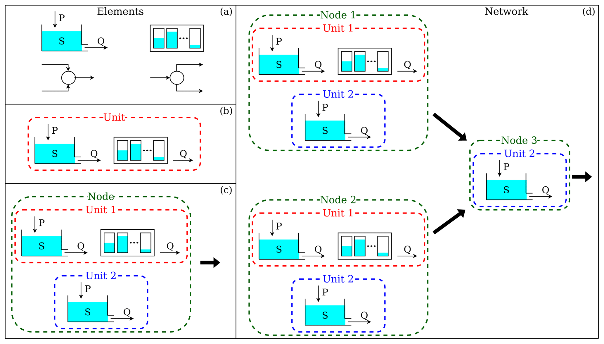
Figure 1 The four hierarchical levels of SuperflexPy and their respective components. (a) Elements (e.g., reservoirs, lags, connections) are used to represent individual hydrological processes/catchment response mechanisms. (b) Units connect multiple elements and are intended to implement lumped catchment models. (c) Nodes collect multiple units that operate in parallel representing different landscape elements within a catchment. (d) Network connects multiple nodes and is used to represent distributed setups.

2 Description of SuperflexPy

2.1 General organization

The SuperflexPy framework has a hierarchical organization with four nested levels: “element”, “unit”, “node”, and “network”, collectively referred as “components”. These components are shown in Fig. 1 and described below. Further practical details are provided in chap. 4 of the Supplement:

1. Element (Fig. 1a). This level represents the basic model building block and is used to create reservoirs, lag functions, and connections. An element can be used to represent an entire catchment or, more commonly, a specific hydrological process or response mechanism within the catchment.

   The reservoir element is used to conceptualize processes involving the storage and release of water and other fluxes. It is described mathematically by ordinary differential equations (ODEs):

   $$\begin{array}{}\text{(1)}& {\displaystyle \frac{\mathrm{d}\mathit{S}\left(t\right)}{\mathrm{d}t}}={\mathit{g}}_S\left(\mathit{S}\left(t\right),\mathit{X}\left(t\right);\mathit{\theta }\right),\text{(2)}& {\displaystyle }\mathit{Y}\left(t\right)={\mathit{g}}_Y\left(\mathit{S}\left(t\right),\mathit{X}\left(t\right);\mathit{\theta }\right),\end{array}$$

   where S is the state variables (e.g., water storages), X is the inputs (e.g., precipitation), Y is the outputs (e.g., streamflow), and g_S and g_Y are specified constitutive functions (e.g., storage–discharge relationships).

   In most conceptual models, reservoir elements have a single state variable (representing water storage); multiple state variables can be accommodated if necessary (e.g., to keep track of snow and liquid water separately). Mathematically, a multi-state reservoir can be represented by a system of differential equations of the form of Eqs. (1) and (2).

   The solution of Eq. (1) is usually obtained numerically using external numerical procedures referred to as “numerical approximators” (see Sect. 4.3).

   The lag function element is used to represent delays in the transmission of the fluxes (e.g., routing). It is described mathematically by a convolution integral:

   $$\begin{array}{}\text{(3)}& \mathit{Y}\left(t\right)=\mathit{X}\left(t\right)\ast {\mathit{g}}_H(t;\mathit{\theta })={\int }_{\mathrm{0}}^T\mathit{X}(t-\mathit{\tau }){\mathit{g}}_H(\mathit{\tau };\mathit{\theta })\mathrm{d}\mathit{\tau },\end{array}$$

   where ∗ denotes the convolution operator, X is the input (e.g., water flux), g_H is the impulse response function, and T is the time of influence of g_H (i.e., the maximum lag).

   There is a general mathematical correspondence between reservoirs and lag functions (e.g., Nash, 1957). SuperflexPy users can select the element specification best suited to their specific context.

   The connection element is used to connect two or more elements whenever a direct connection is not possible. For example, connection elements are used when a flux needs to be split among multiple elements downstream (splitter) or, vice versa, when multiple fluxes need to be aggregated (junction). A particular type of connection is represented by the “transparent” element, which simply outputs the same fluxes it receives as inputs and is used to facilitate the connection between elements (see description of unit below).

   All connection elements are stateless and can be represented mathematically as follows:

   $$\begin{array}{}\text{(4)}& \mathit{Y}\left(t\right)={\mathit{g}}_{\mathrm{C}}\left(\mathit{X}\left(t\right);\mathit{\theta }\right),\end{array}$$

   where g_C describes the connectivity between input fluxes and output fluxes and θ represents connectivity parameters (if any).

2. Unit (Fig. 1b). A unit is a collection of multiple connected elements and is generally intended to implement a lumped catchment model or an HRU in a distributed model. Multiple reservoir and lag function elements within a unit can be connected to each other, either directly (one-to-one connections) or using connection elements such as splitters and junctions (when a single element is connected to multiple elements). The multiple elements within a unit are arranged in layers, with the following restrictions: (i) feedback loops between the elements are not allowed, and (ii) elements can be connected only if they belong to two consecutive layers. Fluxes between elements in nonconsecutive layers are passed using transparent elements. The concept of layers will be elaborated and illustrated in Sect. 5.1.1; see also Sect. 4.2 of the Supplement. In technical terms, the structure formed by the elements must be a directional acyclic graph (DAG). The motivation and implications of these design choices on model generality and computational efficiency are elaborated in Sect. 5.1.1 and 5.2.

3. Node (Fig. 1c). A node is a collection of multiple units that operate in parallel. In the context of distributed models, the node can be used to represent a single catchment and the units can be used to represent multiple landscape elements or HRUs within the catchment. Each unit within a node is characterized by a weight, which typically represents its area fraction or, more generally, its contribution to the total outflow of the node. The weights are used to combine the output fluxes from the units into the total output flux of the node. Another important attribute of a node is its “area”, which is used when multiple nodes are combined into a network (see below).

4. Network (Fig. 1d). A network connects multiple nodes into a tree structure and is typically intended to develop a distributed model that generates predictions at internal sub-catchment locations (e.g., to reflect a nested catchment setup). The network routes the fluxes from upstream nodes (leaves of the tree) to the final downstream node (root of the tree). Routing delays in the river network can be simulated by feeding node outputs into lag function elements. The area of each node is used to determine its contribution to the total outflow of the network. Only a single network can be used in a given SuperflexPy model.

The hierarchical organization of SuperflexPy makes the effort required to configure it to a new problem proportional to the problem complexity. In particular, many common model setups can be constructed without necessarily using all levels listed above, thus reducing configuration effort. Some representative examples are given below:

• Level 1 is sufficient to create single-element models, e.g., a single-reservoir model or a unit hydrograph model (e.g., Kirchner, 2009);

• Level 2 is sufficient to create a lumped model structure, such as GR4J (Perrin et al., 2003) or Hymod (Boyle, 2001);

• Level 3 is sufficient to create a distributed model that represents spatial heterogeneity but generates predictions only at the catchment outlet (e.g., Beven and Kirkby, 1979; Gao et al., 2014; Nijzink et al., 2016);

• Level 4 is needed only in models that generate predictions at interior points, such as SWAT (Arnold et al., 2012), GEOframe-NewAge (Formetta et al., 2014), and distributed SUPERFLEX applications (e.g., Fenicia et al., 2016; Dal Molin et al., 2020).

Examples of SuperflexPy models implemented at levels 2 and 4 are given later in Sect. 3. Note that the association of specific SuperflexPy components to specific hydrological entities, e.g., the use of units for HRUs and nodes for sub-catchments, is not intended as a rigid prescription. Other association choices may be favored by the modeler depending on the required model structure and spatial connectivity.

The clarity of visual model representation is particularly important in flexible frameworks because they can generate many subtly different configurations (e.g., Bancheri et al., 2019). The model schematics in this paper indicate explicitly every element, including reservoirs, lag functions, and junctions (e.g., Fig. 1).

From a software design prospective, SuperflexPy embraces the object-oriented paradigm (e.g., Meyer, 1988). All framework components are represented by objects that can operate either alone or together, interacting with each other and with external libraries (e.g., for calibration) through defined interfaces. More details are provided in Sect. 4.2.

All SuperflexPy components have states and/or parameters, which are controlled programmatically using dedicated methods (refer to Sect. 4.1).

2.2 A simple illustration of SuperflexPy: creating a new model from existing components

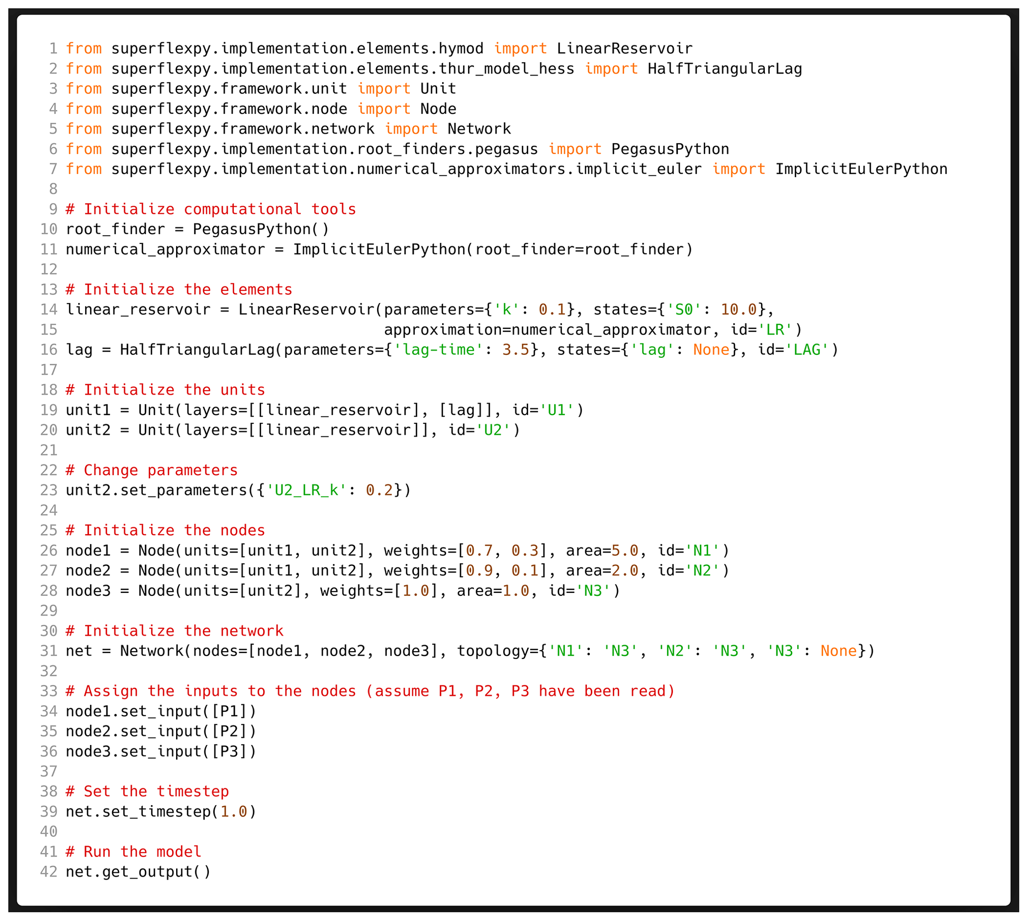
This section illustrates the key steps needed to configure and run a hydrological model using the SuperflexPy framework. The illustration presents a distributed model intended to represent a catchment with two HRUs and three sub-catchments. The model structure is shown in Fig. 1d. The catchment is represented using a network, the sub-catchments are represented using nodes, and the HRUs are represented using units. Two distinct HRU-specific model structures are specified and are implemented using elements. The corresponding SuperflexPy code is shown in Fig. 2. An extended version of this demo is provided in Sect. 6.5 of the Supplement.

Figure 2 SuperflexPy code implementing the simple illustrative model in Fig. 1d.

In this example, an implementation of the necessary elements with SuperflexPy already exists; therefore, the elements only need to be imported. The case where the model structure requires elements for which an implementation is not yet available is considered in Sect. 2.3. More complex setups are described in Sect. 3 and in the Supplement.

We start by importing the model components required by the model structure, namely the elements (LinearReservoir and HalfTriangularLag), unit, node, and network. The numerical approximator ImplicitEulerPython and root finder PegasusPython needed to solve the ODEs associated with the reservoir elements are also imported (see Sect. 4.3 for details). The import operation is shown in lines 1–7.

The imported components are then initialized, which entails specifying the model structure (connectivity between model components) and the initial values of parameters and states. The initialization sequence starts with the numerical procedures (lines 10–11) and proceeds from the lowest-level components (elements) to the highest-level component (network).

Specifically, the following steps apply:

• L1.

  An element is initialized by specifying its parameters, states, and, where relevant, the numerical solver (lines 14–16). Each element is given an identifier (id) for subsequent use, as shown in Line 23.

• L2.

  A unit is initialized by specifying the elements that compose it and the identifier (lines 19–20). As noted earlier in Sect. 2.1, the connectivity between elements is defined by conceptualizing the unit as a succession of layers that contain the elements. More complex examples are given in Sect. 3. The parameters and states of elements can be changed after initialization using the methods set_parameters and set_states of the containing units. This operation is shown in Line 23 for the LinearReservoir element.

• L3.

  A node is initialized by specifying the units that compose it, their contribution (weight) to the node output, the influence area of the node (here, the area of the sub-catchment), and the identifier (lines 26–28).

• L4.

  The network is initialized by specifying the nodes that compose it and their connectivity, called topology (Line 31). The connectivity is defined indicating, for each node, the node downstream of it. A network identifier is not specified (as only a single network can be used).

The next step is to set the model inputs and time step. Lines 34–36 show how the inputs are assigned directly to the nodes, enabling the model to receive spatially varying rainfall and potential evapotranspiration (PET). The time step is set in Line 39 (variable time steps are also supported; see Sect. 4.5.1 of the Supplement).

The model can now be run by calling the get_output method of the highest-level component, as shown in Line 42.

Note that all input quantities provided to SuperflexPy, including fluxes, time step length, parameters, states, and areas, must have consistent units. To reduce model code complexity and execution overhead, we take the perspective that unit checks represent pre-processing and are best handled by the user according to their own preferences and standards. Output fluxes have the same (assumed) units as input fluxes; e.g., if precipitation is in mm/h, then streamflow is also in mm/h.

2.3 Creating new model components with SuperflexPy

We now consider the case where the intended model structure has components beyond those already available in SuperflexPy.

New model components can be created by extending existing SuperflexPy components. To this end, SuperflexPy provides a library of built-in high-level components that can be extended to achieve the desired functionality. We anticipate that the SuperflexPy components most likely to require extension are the elements, where new constitutive functions may be required in reservoir elements and new weight functions may be required in lag function elements. In contrast, it is less likely that unit, node, and network functionalities would require extension.

The extension of existing SuperflexPy elements takes advantage of the object-oriented paradigm underlying the SuperflexPy software design. The inheritance principle, one of the core concepts of the object-oriented paradigm, allows the user to construct new components by “inheriting” most of the functionalities (methods) from existing classes. Separate implementation is then required only for methods where the new model differences are to be introduced. This approach reduces substantially the amount of coding required to implement a new model component.

A detailed example of this procedure is given in Sect. 3.2, which shows how to implement a reservoir with a new storage–discharge relationship. More examples are provided in chap. 8 and 9 of the Supplement.

3 Examples of building hydrological models using SuperflexPy

This section provides more detailed examples of using SuperflexPy to implement hydrological models, including the use of built-in elements and the creation of new elements. We follow a progression from simple to complex. Section 3.1 shows the implementation of model M4, a lumped model built solely from reservoir elements and used in the original SUPERFLEX case study (Kavetski and Fenicia, 2011). Section 3.2 shows how to define a new element with a different storage–discharge relationship for one of the reservoirs of M4. Section 3.3 shows the implementation of a distributed model from a recent application of SUPERFLEX in the Thur catchment (Dal Molin et al., 2020).

Compared to the demo in Sect. 2.2, which was intended to give a general sense of model building with SuperflexPy, the examples in this section represent “realistic” applications of SuperflexPy, including setting up a spatially distributed model with multiple HRUs and more complex model structure. Further technical details and additional examples, including the implementation of popular conceptual models (e.g., GR4J, HYMOD), are provided in the Supplement (chap. 8–11).

3.1 Implementing SUPERFLEX configuration M4

M4 is a simple lumped model presented in Kavetski and Fenicia (2011). As shown in Fig. 3, M4 comprises two reservoirs connected in series: an “unsaturated” reservoir (UR) intended to represent the partitioning of precipitation between evaporation and runoff,and a “fast” reservoir (FR) intended to represent subsequent streamflow generation mechanisms.

Figure 3 Schematic of model M4 used in the original SUPERFLEX case studies of Kavetski and Fenicia (2011).

UR partitions precipitation P^(UR) into a portion that enters the UR storage and eventually evaporates through flux $E_A^{\left(\mathrm{UR}\right)}$ and a portion Q^(UR) that is directed to the downstream FR reservoir:

$$\begin{array}{}\text{(5)}& {\displaystyle \frac{\mathrm{d}{S}^{\left(\mathrm{UR}\right)}}{\mathrm{d}t}}=P^{\left(\mathrm{UR}\right)}-E_A^{\left(\mathrm{UR}\right)}-Q^{\left(\mathrm{UR}\right)},\end{array}$$

where

$$\begin{array}{}\text{(6)}& {\displaystyle }{\stackrel{\mathrm{‾}}{S}}^{\left(\mathrm{UR}\right)}={\displaystyle \frac{S^{\left(\mathrm{UR}\right)}}{S_{\max }^{\left(\mathrm{UR}\right)}}},\text{(7)}& {\displaystyle }{Q}^{\left(\mathrm{UR}\right)}=P^{\left(\mathrm{UR}\right)}\times {\left({\stackrel{\mathrm{‾}}{S}}^{\left(\mathrm{UR}\right)}\right)}^{{\mathit{\beta }}^{\left(\mathrm{UR}\right)}},\text{(8)}& {\displaystyle }{E}_A^{\left(\mathrm{UR}\right)}=E_P^{\left(\mathrm{UR}\right)}\times {\displaystyle \frac{{\stackrel{\mathrm{‾}}{S}}^{\left(\mathrm{UR}\right)}\left(\mathrm{1}+m^{\left(\mathrm{UR}\right)}\right)}{{\stackrel{\mathrm{‾}}{S}}^{\left(\mathrm{UR}\right)}+m^{\left(\mathrm{UR}\right)}}}.\end{array}$$

In Eqs. (6)–(8), $S_{\max }^{\left(\mathrm{UR}\right)}$ and β^(UR) are model parameters. The quantity m^(UR) is used to approximate a “smooth” threshold behavior; we typically fix m^(UR)=0.01.

FR is a power-law reservoir:

$$\begin{array}{}\text{(9)}& {\displaystyle \frac{\mathrm{d}{S}^{\left(\mathrm{FR}\right)}}{\mathrm{d}t}}=P^{\left(\mathrm{FR}\right)}-Q^{\left(\mathrm{FR}\right)},\end{array}$$

with the storage–discharge relationship given by

$$\begin{array}{}\text{(10)}& Q^{\left(\mathrm{FR}\right)}=k^{\left(\mathrm{FR}\right)}{\left(S^{\left(\mathrm{FR}\right)}\right)}^{{\mathit{\alpha }}^{\left(\mathrm{FR}\right)}},\end{array}$$

where k^(FR) and α^(FR) are model parameters.

The inflow P^(FR) is given by the outflow from UR; i.e., P^(FR)=Q^(UR).

M4 is a lumped model with multiple elements and hence can be implemented using SuperflexPy levels L1 and L2 (element and unit; see Sect. 2.1). Figure 4 shows the code needed to implement M4. The numerical procedures are imported and initialized in lines 1–2 and 7–8, respectively. Similar to the model described in Sect. 2.2, the two model elements (UR and FR) are already implemented. Hence, the user only needs to import the elements (lines 1–3) and initialize their parameters (lines 7–13). Next, the unit is imported (Line 4) and initialized to contain the two reservoirs (Line 15). The model configuration is then complete.

Figure 4 SuperflexPy code implementing model M4 in Fig. 3.

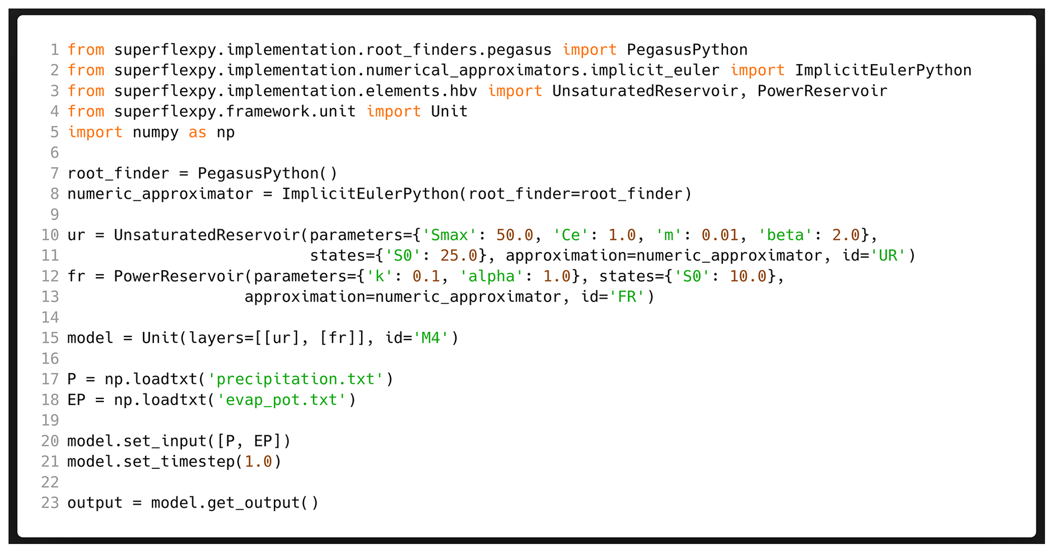
The loading of input data from text file(s), databases, etc., is separate from the configuration of SuperflexPy and can be carried out using any suitable Python library or function. In this example, we use NumPy to read time series of precipitation and PET from a text file, as shown in lines 17–18. The corresponding SuperflexPy inputs are set using these NumPy arrays, as shown in Line 20. Further practical details on input–output are provided in Sect. 4.5.5 of the Supplement.

The model can now be run with the given input data to produce the model outputs, as shown in Line 23. The outputs contain streamflow time series in the form of NumPy arrays.

3.2 Changing the equations of the fast reservoir in M4

Suppose the modeler wishes to modify model M4 by changing the storage–discharge equation of the fast reservoir given in Eq. (10) to a new relationship:

$$\begin{array}{}\text{(11)}& Q^{\left(\mathrm{FR}\right)}={\displaystyle \frac{k^{\left(\mathrm{FR}\right)}{\left(S^{\left(\mathrm{FR}\right)}\right)}^{{\mathit{\alpha }}^{\left(\mathrm{FR}\right)}}}{S^{\left(\mathrm{FR}\right)}+b^{\left(\mathrm{FR}\right)}}},\end{array}$$

where k^(FR), α^(FR), and b^(FR) are model parameters.

An element with this storage–discharge relationship has not been implemented in SuperflexPy yet (as of version 1.3.0). The following sections give two approaches for creating such an element.

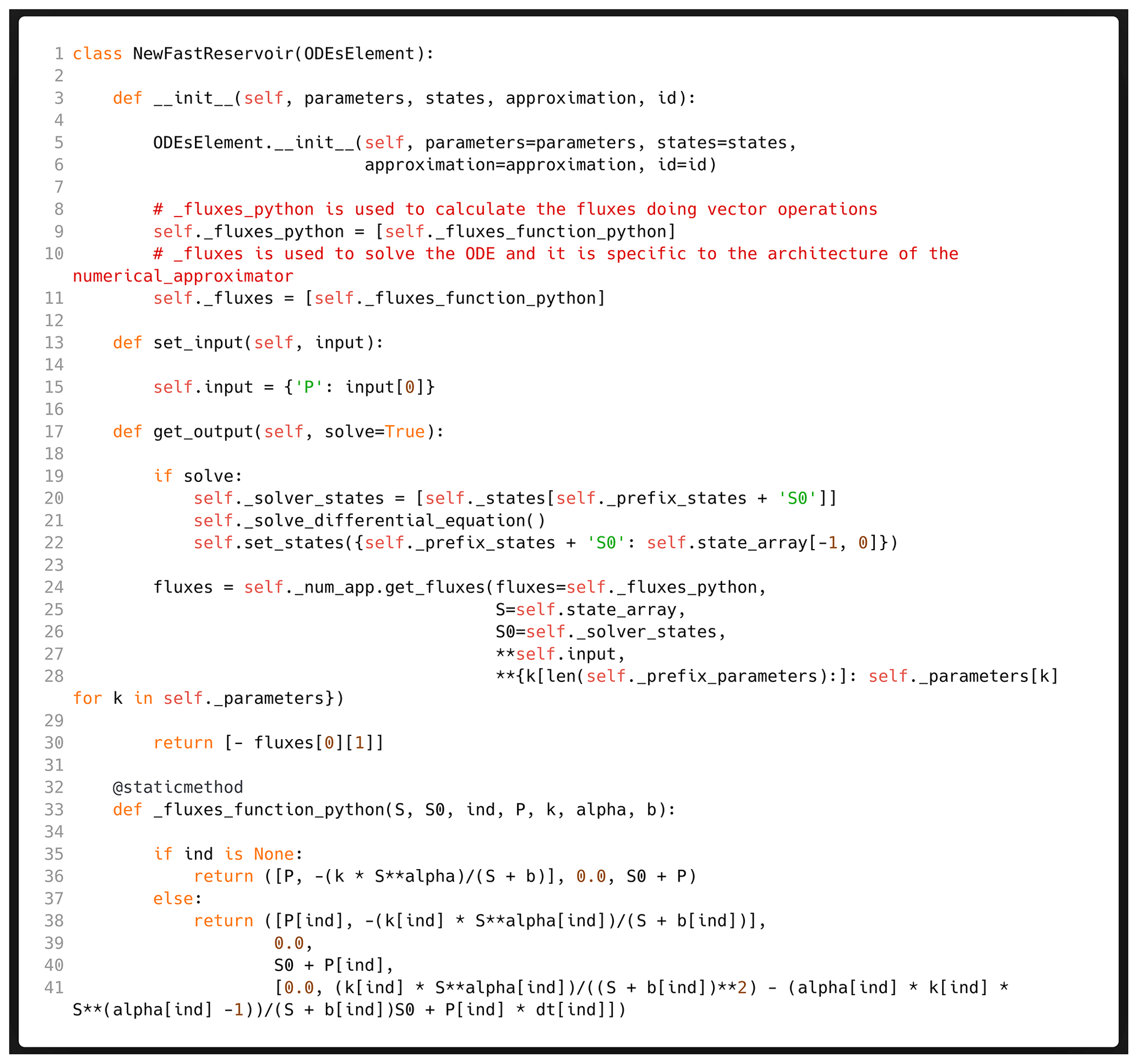
Figure 5 General approach for implementing a new reservoir element NewFastReservoir by extending the class ODEsElement (Sect. 3.2.1).

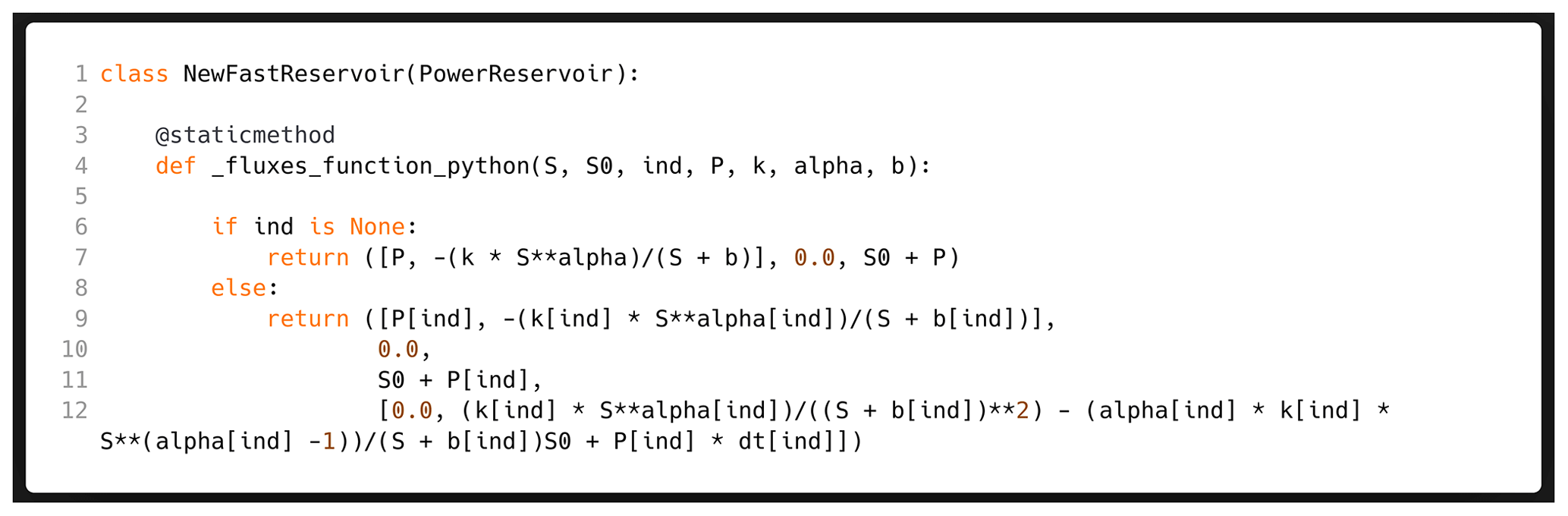
Figure 6 Simplified approach for implementing the NewFastReservoir by inheriting directly from class PowerReservoir (Sect. 3.2.2).

3.2.1 General approach for creating a new reservoir with SuperflexPy

The general approach for creating a new reservoir in SuperflexPy is to define a new class that inherits most of its functionality (methods) from the class ODEsElement. This operation is illustrated in the code snippet in Fig. 5 (see Sect. 8.1 of the Supplement for full details). The new class must override the following methods:

• __init__ is the constructor of the class. Its main purpose is to invoke the constructor of the parent class (lines 5–6) and to point to the method used to calculate the fluxes, here, _fluxes_function_python (see also Sect. 4.3, which illustrates the efficiency benefits of using Numba-optimized methods for calculating the fluxes).

• set_input takes the input fluxes in a predefined order (here, just precipitation) and assigns them a key (Line 15) that is then used when setting up and solving the model equations,

• get_output invokes the functionalities implemented by the ODEsElement to solve the element equation over the entire simulation (all time steps). Lines 20–22 get the current state of the reservoir, invoke the ODE solver, and set the state to its final value. Lines 24–28 get the output flux arrays from the numerical approximator (see Sect. 4.3). Line 30 returns a list with the output of the element (here, the streamflow).

• _fluxes_function_python calculates the fluxes and (optionally) their derivatives with respect to the state for a given state, inputs, and parameters. Line 36 implements the vector version while lines 38–41 implement the scalar version. Both versions are needed by the numerical approximator (see Sect. 4.3; further practical details are provided in Sect. 8.1 of the Supplement).

The new element NewFastReservoir is now defined and can be used in the “new” version of M4, in lieu of the previous element PowerReservoir. The object-oriented features of Python are very useful here to enable the new class NewFastReservoir to inherit most of the methods from the base class ODEsElement. Otherwise, in addition to the methods listed above, we would have needed to implement many other methods, e.g., for interfacing with numerical solvers and for setting element parameters and states.

3.2.2 Simplified approach for creating a new reservoir element (from an existing element)

The same new reservoir element can be implemented in a simpler way by noting that NewFastReservoir differs from PowerReservoir solely in the definition of the outflow equation. This difference affects only one of the four methods implemented in Fig. 5, namely _fluxes_function_python. A simpler implementation of NewFastReservoir can be therefore achieved by inheriting this class directly from class PowerReservoir rather than from class ODEsElement. The code in Fig. 6 illustrates this approach and implements only the method _fluxes_ function_python. All other methods are inherited from class PowerReservoir.

Note that this simplified implementation is a consequence of the required modification being relatively minor, i.e., a change solely in the constitutive function equation. More complex modifications, such as the inclusion/exclusion of input/output fluxes (e.g., inclusion of evapotranspiration into the PowerReservoir), would require the general implementation approach described in Sect. 3.2.1.

3.3 Implementing a distributed model

This section illustrates the implementation of an HRU-based, distributed hydrological model, intended to simulate streamflow in a nested catchment. This implementation requires the entire workflow illustrated in Sect. 2.2. The example is provided by model M02, developed in Dal Molin et al. (2020), to provide streamflow predictions at 10 sub-catchments of the Thur catchment in Switzerland (Fig. 7a).

Each sub-catchment receives its own forcing, namely precipitation, potential evapotranspiration, and temperature. Two HRU types are defined based on geology: consolidated and unconsolidated formations (Fig. 7b). Both HRU types are characterized by the same model structure, which is shown in Fig. 8. This HRU model structure differs from model structure M4 (Sect. 3.1) in the following additional elements: (i) a “snow” reservoir, WR, which controls the partition of incoming precipitation between rainfall and snowfall based on temperature, (ii) a lag function between UR and FR, and (iii) a “slow” reservoir, SR, which acts in parallel to FR and is controlled by the same equations as FR but with different parameter values.

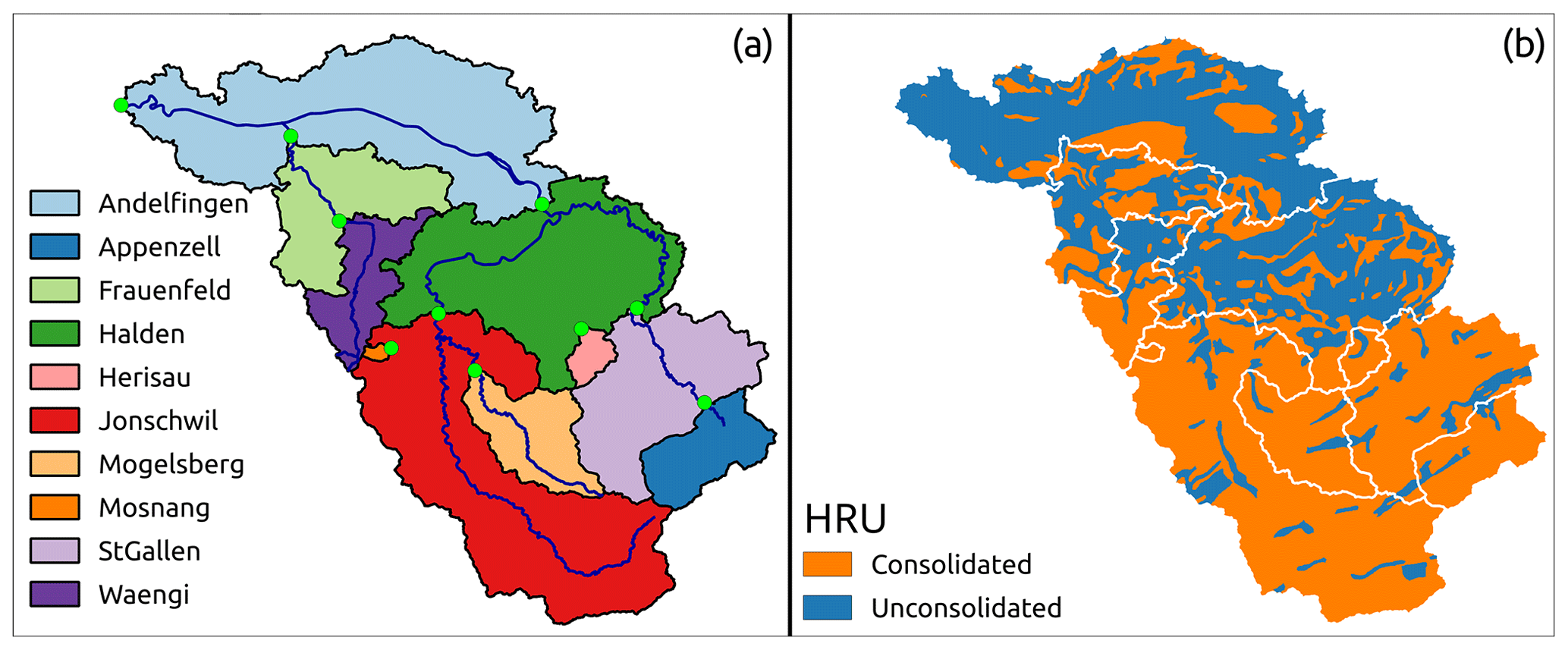
Figure 7 Illustration of catchment discretization used for a distributed application of SuperflexPy in the Thur catchment: (a) discretization into sub-catchments and (b) discretization into hydrological response units (HRUs) as presented in model M02 in Dal Molin et al. (2020). The panels of this figure were originally published in Figs. 1a and 6 of Dal Molin et al. (2020). The HRU model structure is shown in Fig. 8.

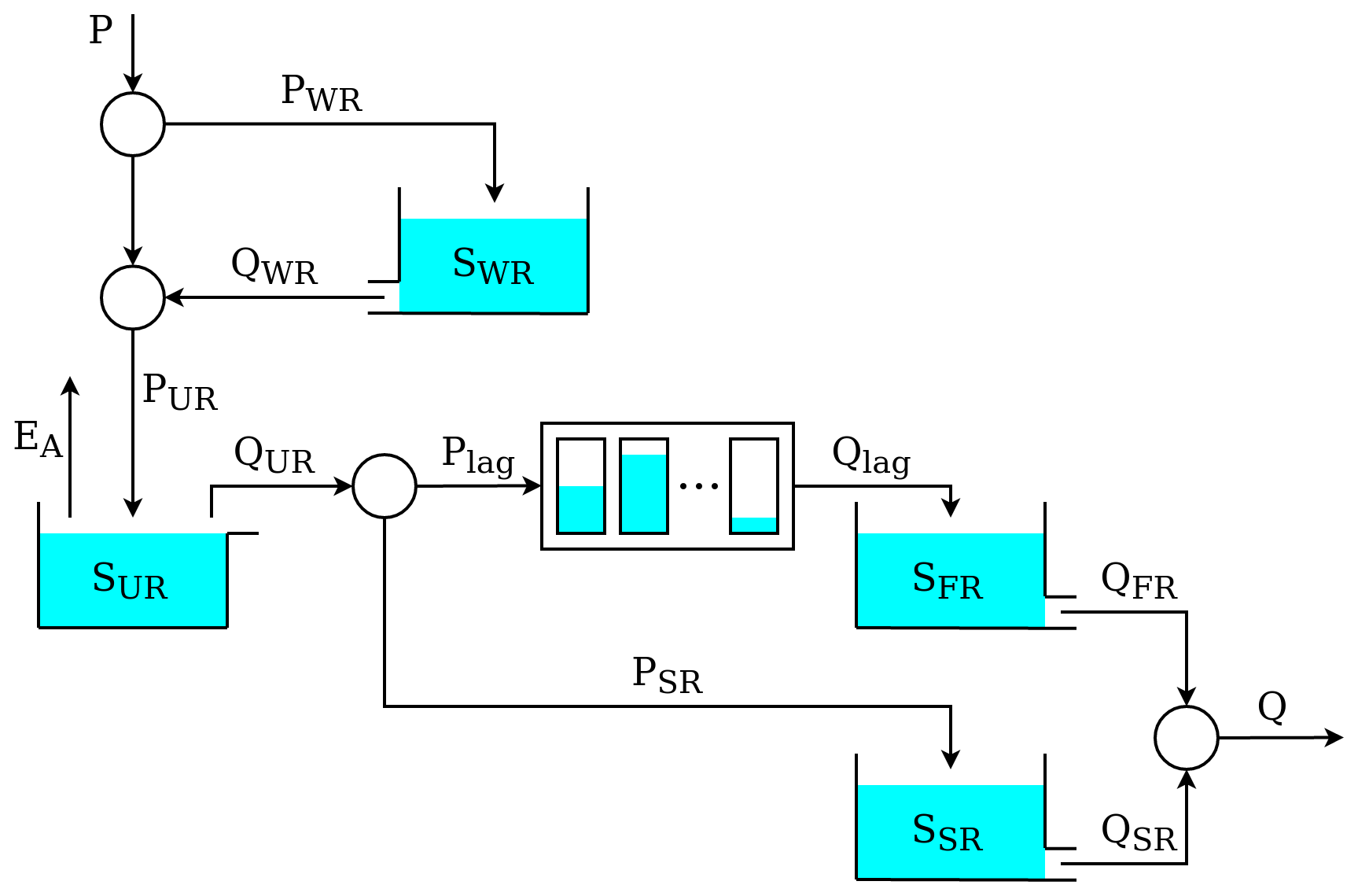
Figure 8 Model structure used to represent the HRUs in model M02 in Dal Molin et al. (2020). Refer to Fig. 7 for the corresponding HRU discretization of the Thur catchment.

Similar to the simpler previous example in Sect. 3.1, this “lumped” model structure is implemented as a unit. However, a key difference is that in the previous example the unit represented the entire system, whereas here it is part of a more complex system.

Given the spatial organization of the model, nodes are used to represent sub-catchments and units are used to implement HRU types. Note that the sub-catchments may share (one or more) HRU types, which in SuperflexPy translates into the nodes sharing (one or more) units. The network level is used to connect multiple nodes and enables predictions at internal catchment locations. Figure 10 shows the SuperflexPy representation of the spatial organization shown in Fig. 7.

We start by implementing the units. As seen in Fig. 8, the HRU model structure has elements operating in parallel and, therefore, requires the use of connections. Figure 9 shows how the HRU model structure is “translated” into a SuperflexPy unit. Recall, from Sect. 2.1, that elements can be connected only if they belong to two consecutive layers, which implies that “gaps” in the structure must be filled using transparent elements, which output the same fluxes they receive as inputs. Splitters and junctions are used to divide and merge the fluxes to implement the parallel flow paths.

Figure 9 SuperflexPy representation of the model structure M02 in Fig. 8.

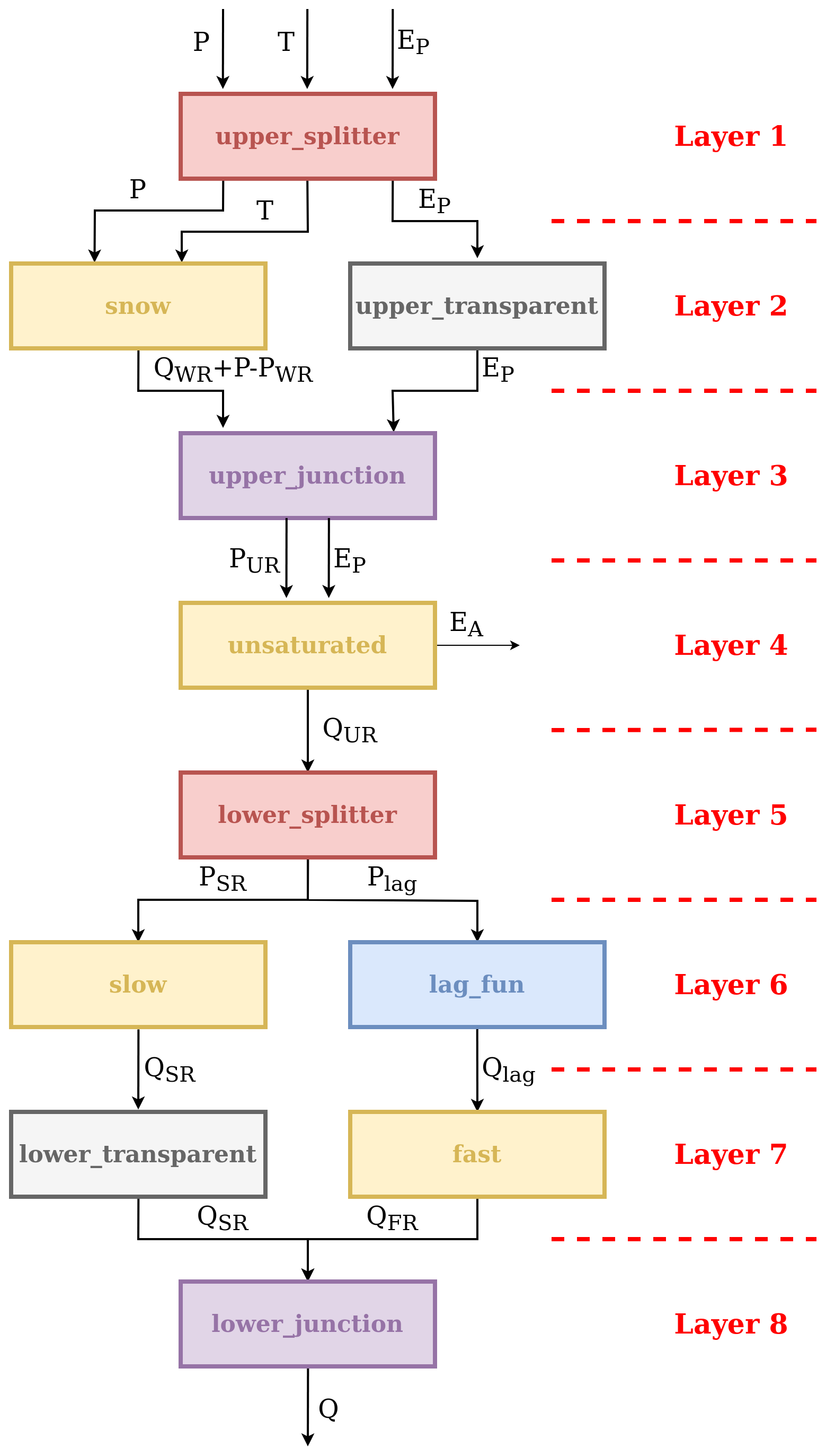
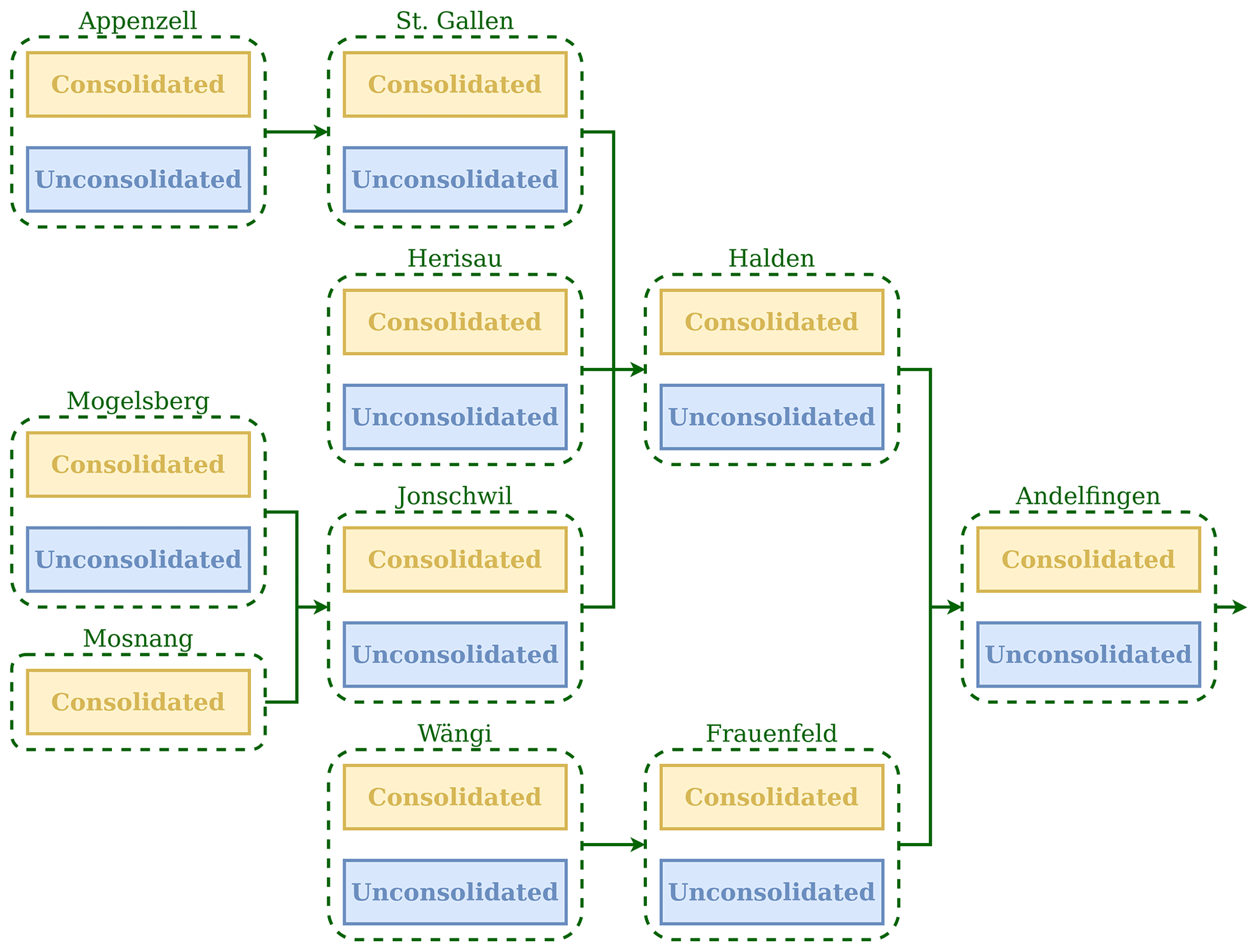
Figure 10 Spatial organization of the SuperflexPy model configuration used to simulate water fluxes in the Thur catchment (M02 in Dal Molin et al., 2020). The units, used to represent the HRUs, are shown using the blue and yellow boxes. The nodes, used to represent the sub-catchments, are shown using the green dashed boxes. The group of nodes connected together (green arrows) creates a network.

Comparing Fig. 8 with Fig. 9, we see how the HRU structure has been implemented within SuperflexPy. The following implementation aspects are noted:

1. The incoming precipitation is partitioned into rainfall and snowfall. This partitioning is done internally in the WR element. The SuperflexPy implementation of WR takes care of two processes: (i) partitioning of precipitation into rainfall and snowfall and (ii) simulation of snow processes (accumulation and melting). The output of WR is, logically, the sum of rainfall and snowmelt. Alternatively, a (new) splitter element could have been defined to partition the fluxes between UR (rainfall) and WR (snowfall) based on temperature.

2. WR, as currently implemented, does not receive as input PET, which is needed by the downstream element UR. Therefore, the transfer of PET values to the UR element is implemented using a separate path composed of three elements, labeled “upper splitter”, “upper transparent”, and “upper junction” (Fig. 9). This choice simplifies the interface of element WR at the expense of a somewhat more complicated model structure with additional elements.

3. The parallel part of the structure is composed of two elements on one branch (lag and FR) and only one element on the other branch (SR). To satisfy the requirement of not having gaps in the unit structure, a transparent element (lower_transparent) is added after the SR.

The code to set up this model is detailed in Fig. 11. Similar to the earlier example in Sect. 2.2, the user initializes and connects all model components, proceeding sequentially from the lowest level (elements) to the highest level (network). The procedure can be summarized as follows:

1. lines 10–29 – initialize the elements needed for the lumped model structures used in the HRUs;

2. lines 32–39 – initialize the units used to represent the HRUs, linking all the elements;

3. lines 42–51 – initialize the nodes used to represent the sub-catchments; both units are assigned to nine nodes; the Mosnang sub-catchment contains a single HRU, and hence only a single unit is assigned to the corresponding node (Line 49);

4. lines 54–60 – connect the nodes using a network; the topology of the network is defined by indicating, for each node, the downstream one.

The network runs the nodes from upstream to downstream, collects their outputs, and routes them to the outlet. Customized routing functions can be implemented, as shown in Sect. 9.1 of the Supplement. The output of the network is a Python dictionary, with keys given by the node identifiers and values given by the list of NumPy arrays representing the time series of output fluxes over the simulation period.

4 Implementation details of SuperflexPy

This section presents additional technical details of SuperflexPy needed to understand better some aspects of the functioning of the framework. A more detailed and practical description is provided in the Supplement.

4.1 Parameters and states

All SuperflexPy components can have parameters and states. Parameters specify component characteristics, whereas states keep track of the component history. States and parameters are set as part of initializing the model components and can be manipulated using get and set methods provided by the framework at all levels of its hierarchy (see the example in Sect. 2.2).

The parameters can be either constant or variable in time. Constant parameters represent the most common setup of hydrological models. In conceptual hydrological modeling, time-varying parameters have been proposed to represent ”deterministic” system variability (e.g., seasonality, Westra et al., 2014) and/or “stochastic” system variability (e.g., Kuczera et al., 2006; Reichert and Mieleitner, 2009; Renard et al., 2011); see also earlier work in data-based mechanistic modeling (e.g., Young, 2000).

Figure 11 SuperflexPy code implementing the distributed model in Figs. 9 and 10.

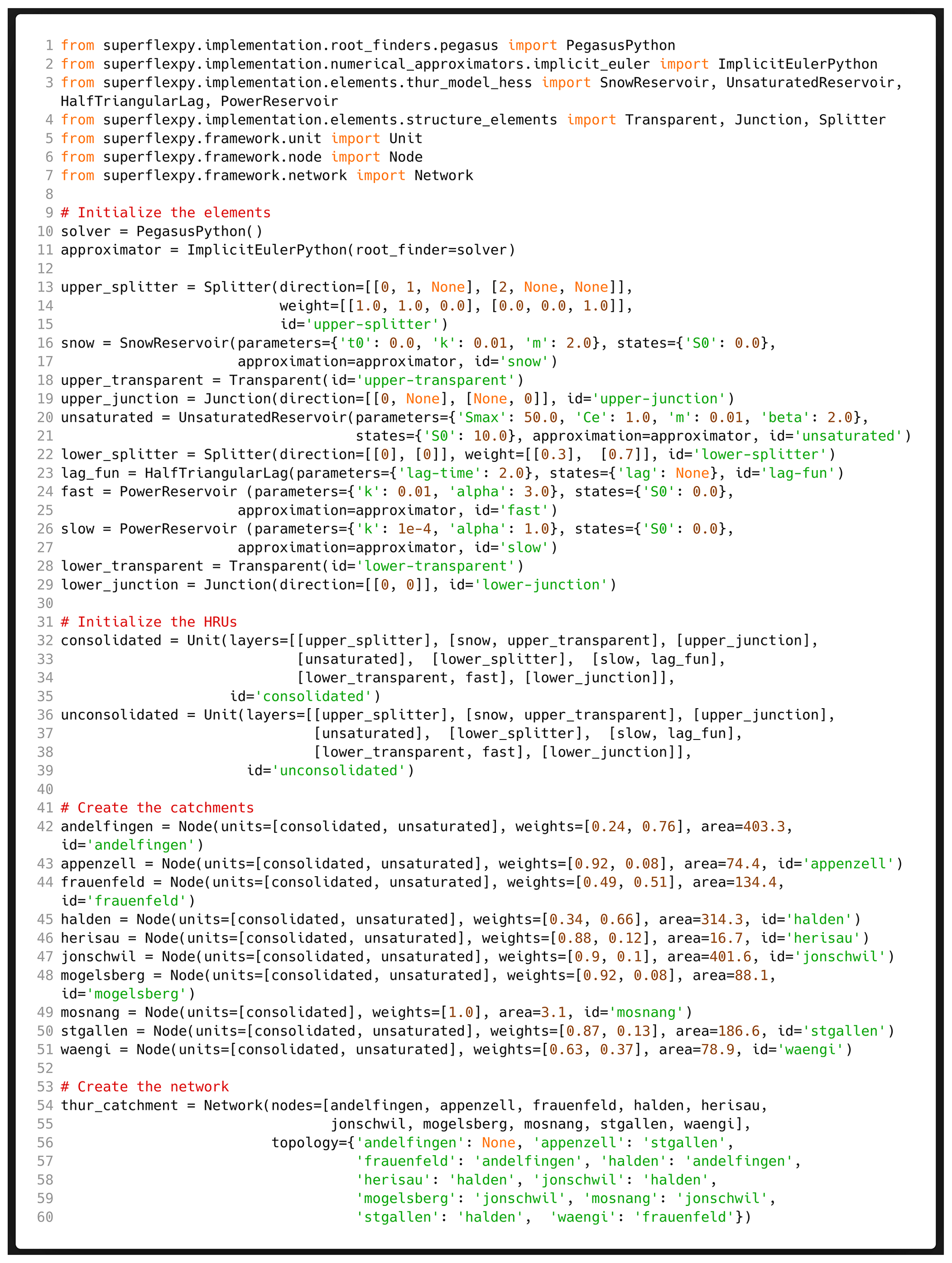
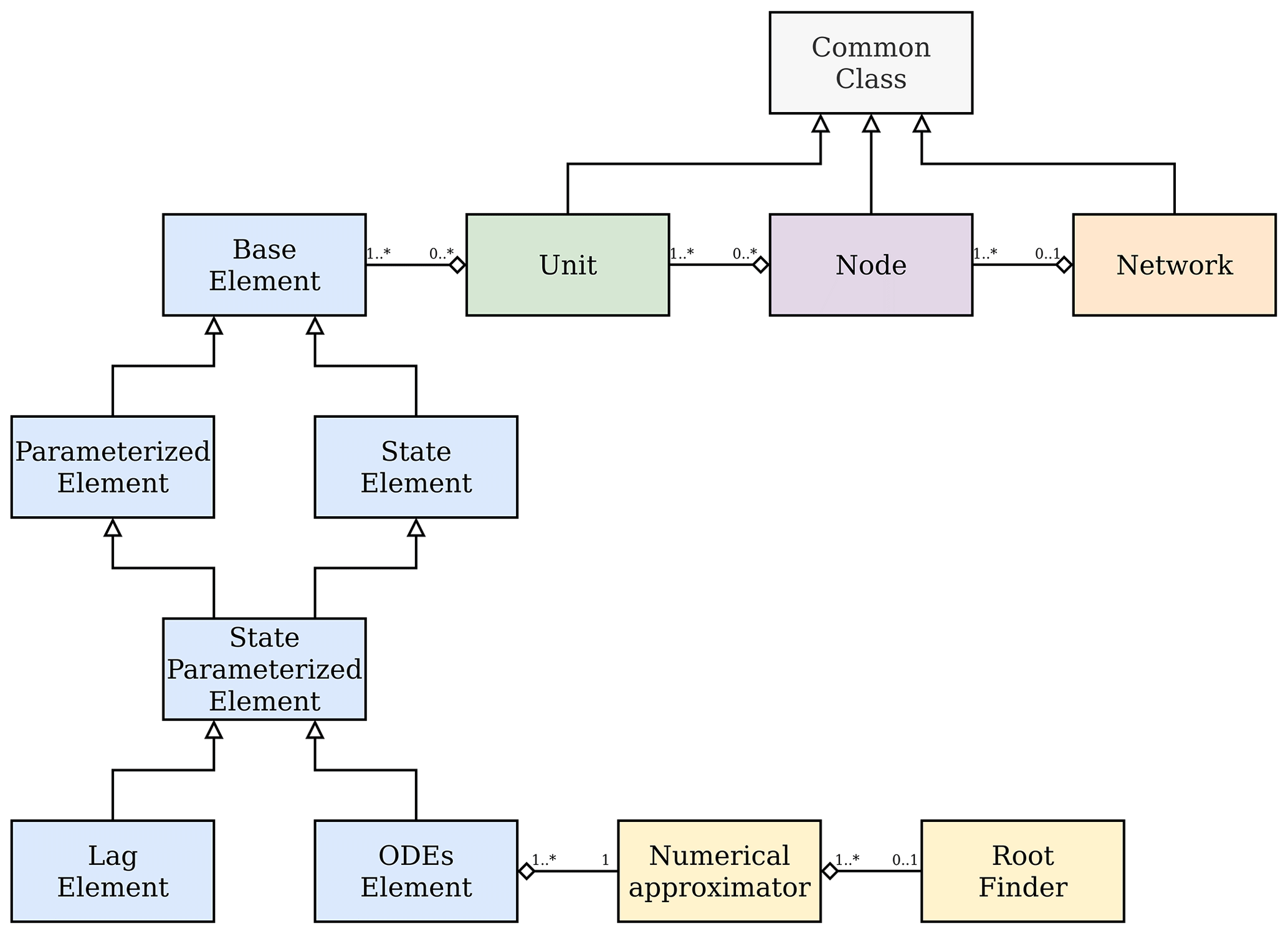
Figure 12 UML class diagram showing the organization of the classes used to represent SuperflexPy components. The core framework is presented, excluding the specific implementations of components and numerical routines.

4.2 Modular design following the object-oriented paradigm

As noted in Sect. 2.1, SuperflexPy embraces the object-oriented paradigm (e.g., Meyer, 1988), which is widely used in general software and is increasingly adopted in scientific software.

Figure 12 shows the unified modeling language (UML) class diagram of SuperflexPy. The schematic illustrates the classes underlying the core framework (i.e., the base classes that define SuperflexPy architecture) but excludes, for simplicity, the specific implementations of components and numerical routines. All the classes in the diagram can be extended to implement customized components; for example, a reservoir can be implemented by extending the class ODEsElement, a splitter can be implemented by extending the class ParameterizedElement, and a node with a particular routing mechanism can be implemented by extending the class Node.

The object-oriented design provides several advantages in the context of SuperflexPy:

• The inheritance principle enables the creation of new classes by extending existing ones. Inheritance reduces drastically the amount of new code that needs to be generated to implement a new model component (see example in Sect. 3.2).

• Changes to a class (e.g., a component) and the creation of new classes can be carried out in isolation from the rest of the code, as long as the interfaces between classes are respected.

• When creating a model, only the necessary objects need to be initialized and used. This principle makes the model configuration effort roughly proportional to required model complexity; i.e., simple model structures can be constructed from the minimal set of required components.

• Objects retain their history (states), which can be accessed post-run to undertake model analysis and/or subsequent computation.

• The modular nature of objects facilitates the development and testing of new code.

These benefits make it easier to achieve clean and maintainable code, which is essential for any practical modeling framework.

4.3 Numerical solution of ODEs

The mass balance of reservoir elements is described using ordinary differential equations (ODEs), which are typically solved (approximately) using numerical time stepping algorithms. Many such algorithms have been described in the numerical methods literature, e.g., Euler methods, Runge–Kutta methods (e.g., Butcher and Goodwin, 2008).

SuperflexPy separates the formulation of model equations from the solution of these equations. Specifically, flux equations are defined internally as methods of the elements (as shown in Sect. 3.2), while the numerical algorithm to solve the ODEs is specified externally to the element, creating a class specific to this task. The separation of equations and solvers in the model specification enables the modeler, within some restrictions, to select the numerical method without making any changes to the governing model equations (see Sect. 5.2 of the Supplement). That said, given SuperflexPy's primary emphasis on enabling hydrologists to experiment with flexible conceptual model structures, numerical flexibility is given a relatively lower level of priority and the choice of numerical architecture of the framework is largely driven by findings of previous studies (see below).

SuperflexPy conceptualizes the solution of its mass balance ODEs as a two-step process: (1) construct a discrete-time numerical approximation of the ODEs (e.g., using Euler time stepping schemes), and (2) when an implicit time stepping scheme is used, solve the associated nonlinear algebraic equation(s). The procedures used for these tasks are referred to as the “numerical approximator” and the “root finder”, respectively. This distinction helps achieve better software modularization, disentangling the choice of the numerical approximator and of the root finder.

Currently, SuperflexPy provides three built-in numerical approximators, namely the fixed-step implicit and explicit Euler time stepping schemes (e.g., Clark and Kavetski, 2010) and Runge–Kutta 4. Two built-in root finders are provided, namely the Pegasus algorithm (Dowell and Jarratt, 1972) and a hybrid Newton–bisection algorithm (Press et al., 1992). Additional numerical routines are currently being developed. To avoid mass balance discontinuities, as well as to ensure better numerical stability and faster convergence, we recommend using smooth flux functions (e.g., Kavetski and Kuczera, 2007).

An additional approximation is employed within SuperflexPy, namely that all model fluxes are constant within the model time step. This approximation is consistent with the typical format of hydrological data, such as rainfall and PET, which are tabulated in discrete steps (e.g., daily, hourly), but is applied not only to the forcing data but also to all internal fluxes. As such, this pragmatic approximation enables a further simplification of the solution procedure because the output flux from each element becomes a scalar value (per time step). Note that first-order time stepping schemes, which we recommend for SuperflexPy, themselves make exactly the same assumption and are hence not impacted. However, higher-order time stepping schemes and adaptive substepping schemes would be impacted by additional first-order discretization error because the variation in internal fluxes within the model time step is ignored. Further details about this pragmatic approximation are provided in Sect. 5.2 of the Supplement.

The user can implement additional numerical algorithms, either by coding them directly or by interfacing with external code (e.g., ODE solvers from SciPy). Detailed instructions are provided in Sect. 5.1 of the Supplement, which also includes a description of how to implement a numerical solver “from scratch”, bypassing the current numerical approximator and/or root finder architecture.

As detailed next in Sect. 4.4, the choice of numerical implementation, and its compatibility with optimizing compilers, may have a strong impact on the overall computational speed of the model.

4.4 Computational efficiency and language choice

Computational efficiency is a key requirement of a practical modeling framework. Model calibration via parameter optimization is a common computationally demanding task required by most hydrological models, typically requiring hundreds or thousands of model runs. Moreover, conceptual hydrological models are often used in Monte Carlo uncertainty quantification, with comparable or even larger computational cost (up to millions of model runs in some cases).

The choice of programming language inevitably requires tradeoffs between computational efficiency and ease of use. The choice of Python for SuperflexPy was motivated by the attraction of a flexible and widely used scripting language in conjunction with two efficient numerical libraries: NumPy (Walt et al., 2011) and Numba (Lam et al., 2015). NumPy provides highly efficient arrays for vectorized operations (i.e., element-wise operations between arrays). Numba provides a “just-in-time compiler” that compiles (at runtime) a Python method into machine code that interacts efficiently with NumPy arrays.

The combined use of NumPy and Numba is particularly effective when solving ODEs, where the numerical algorithm performs element-wise sequential operations. The built-in SuperflexPy approaches for solving ODEs are compatible with such numerical infrastructure and therefore enable fast computation times. Note that switching to ODE solvers that do not take advantage of such libraries might dramatically increase the model runtime.

Numba offers drastic computational speedups compared to native Python; our experimentation suggests runtime reductions by factors of up to 30. However, a drawback of Numba is the requirement to compile the code each time it is executed (run). For a lumped model composed of a few reservoirs, the Numba compilation time is of the order of a few seconds. Therefore, Numba will outperform Python when the simulation is long (e.g., multiple years of hourly data) and/or when the model needs to be run a large number of times. For example, as a broad illustration of runtimes on a standard laptop, calibration of a HYMOD-like SuperflexPy model to observed daily data, requiring 1000s of model runs each with 1000 time steps, takes a few seconds with the Numba implementation compared to a couple of minutes with native Python execution. Note that here we refer to the runtime of the SuperflexPy model itself and exclude the runtime of the calibration tool procedures; more details on benchmarking are given in Sect. 5.3 of the Supplement. Examples of the interoperability of SuperflexPy with external libraries for model calibration (e.g., SPOTPY, Houska et al., 2015) are given in chap. 14 of the Supplement.

4.5 Ability to represent multiple fluxes and states

SuperflexPy can operate with multiple fluxes and state variables. In particular, connection elements, units, nodes, and the network can accommodate an arbitrarily large number of fluxes. The use of multiple fluxes has been already shown in the model structure described in Sect. 3.3, where the upper_splitter handles three different variables (precipitation, temperature, and PET). Additional examples are provided in the Supplement (e.g., chap. 10, 11).

The capability to simulate multiple fluxes and states is intended to support the future extension of SuperflexPy to new modeling scenarios. Several such scenarios may be of interest, including the transport of chemical substances (e.g., Fenicia et al., 2010; Ammann et al., 2020), the interaction between frozen and liquid water in a snow element (e.g., Jansen et al., 2021), and interactions in the saturated and unsaturated soil zones (e.g., Seibert et al., 2003).

While the current examples in SuperflexPy do not include all the cases listed above, the framework architecture anticipates the need for more general simulation functionality and has been designed to support extension to accommodate such multi-state processes.

5 Discussion

5.1 Balancing functionality, scope, and usability in a flexible model implementation

A software implementation that maximizes flexibility and usability is challenging to achieve because flexible modeling functionality may increase configuration effort and computational cost. Existing flexible frameworks have approached this tradeoff with different priorities, based on their respective modeling objectives and paradigms.

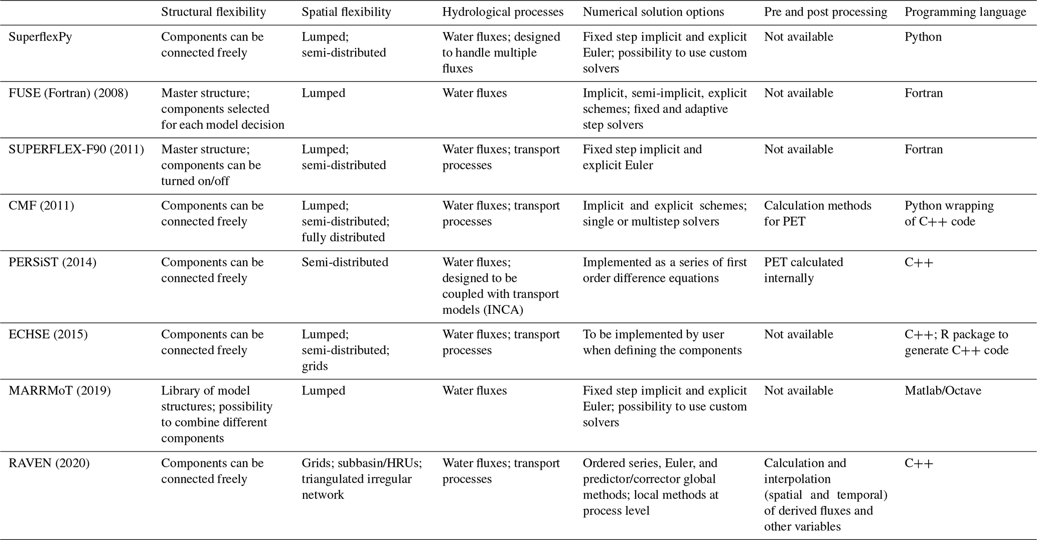
The following sections offer a brief discussion of the design choices made by SuperflexPy in the context of selected existing frameworks with a similar scope. The discussion makes use of Tables 1 and 2, which summarize key design choices related to usability and simulation capabilities, respectively.

Table 1 Summary of usability characteristics of SuperflexPy in the context of selected flexible frameworks for conceptual hydrological modeling.^*

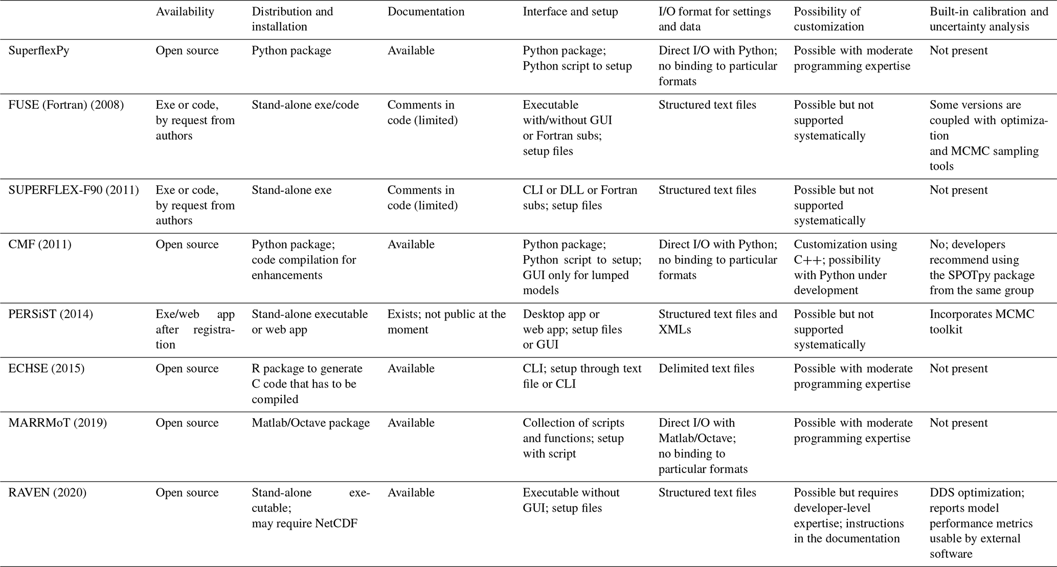
^* This information was collated based on published information. A brief informal review was provided by the framework developers. Abbreviations: exe – binary executable; subs – subroutines; GUI – graphical user interface; CLI – command line interface; DLL – dynamic link library; MCMC – Monte Carlo Markov Chain; DDS – dynamic dimensioned search.

Table 2 Summary of simulation capabilities of SuperflexPy in the context of selected flexible frameworks for conceptual hydrological modeling.^*

^* This information was collated based on published information. A brief informal review was provided by the framework developers.

5.1.1 Structural flexibility

Structural flexibility refers to the flexibility in how elements can be connected to compose the structure of the model (i.e., of the unit, following SuperflexPy terminology). This consideration applies both to lumped and distributed models; the flexibility in specifying the spatial organization of the model is considered separately in Sect. 5.1.2.

Some flexible frameworks are implemented using a master structure that incorporates all supported model configurations. In these implementations, the user can choose the flux equation(s) (e.g., FUSE, SUPERFLEX-F90) and/or activate/deactivate specific elements (e.g., SUPERFLEX-F90) but cannot change the overall connectivity of model elements. To the extent that the master structure is sufficiently general, it may not unduly restrict the practical usage of the framework.

Other frameworks (e.g., MARRMoT) propose a collection of existing conceptual model structures ready to use, which have been implemented following the same design rules in order to allow for a fair comparison. Such frameworks are typically intended for model intercomparison studies.

The most general frameworks allow connecting the elements freely without constraints. A distinction can be made between frameworks that allow for mutual interactions between the elements (e.g., CMF) and frameworks that do not allow such interactions (e.g., ECHSE).

SuperflexPy adopts the latter philosophy, allowing us to connect the elements freely within the unit but restricting mutual interactions, i.e., constraining the structure to be a DAG (see Sect. 5.2). Moreover, we have chosen to define the DAG as a succession of layers, listing the elements in order from upstream to downstream and allowing for parallel flow paths (e.g., see the model structure in Fig. 9). This “list” formulation has been selected in preference to other methods for defining a graph, e.g., connectivity matrix or adjacency list, for the following reasons: (i) simplicity and scalability, as the list dimension scales linearly with the number of elements, in contrast to the connectivity matrix approach where this scaling is quadratic; (ii) arguably better readability, as the elements are listed in the order they appear in the DAG; and (iii) it guarantees a graph topology without loops. Note that other popular modeling tools (e.g., neural networks) adopt this type of formulation.

5.1.2 Spatial flexibility

Most frameworks (e.g., CMF, ECHSE, SUPERFLEX-F90) support multiple types of spatial discretization (e.g., lumped, HRUs, sub-catchments, grids). Some frameworks (e.g., FUSE, MARRMoT) support solely lumped models.

SuperflexPy uses four hierarchical levels of components, intended to facilitate the formulation of models that range in spatial complexity from a simple lumped model to a composition of lumped models intended for prediction at a single location (e.g., a catchment with several HRUs) and ultimately to a distributed model capable of making predictions at multiple internal locations. The use of a hierarchical set of components could be contrasted with a framework based solely on the lowest-level components, here, elements. The use of higher-level components enables the modeler to capture explicitly the natural groupings in the catchment of interest, e.g., sub-catchments and HRUs.

5.1.3 Usability

The usability of a framework can be judged according to several aspects.

The first aspect is how a framework is operated. Some frameworks are stand-alone and operated through a graphical interface (e.g., PERSiST) or the command line interface (e.g., SUPERFLEX-F90). Other frameworks are designed as libraries that can be called from the user code in a specific programming language to initialize, configure, and run the model (e.g., CMF, MARRMoT; SUPERFLEX-F90 also allows this option when using the source code from Fortran). SuperflexPy is implemented as a Python package. Models can be created using a Python script and interfaced easily with external libraries (examples are provided in chap. 14 of the Supplement).

The second aspect is the scope of the framework. Most frameworks (e.g., SUPERFLEX-F90, ECHSE) adopt, by design, the philosophy of “one tool per problem” and limit their functionality to the simulation of hydrological processes. Other frameworks integrate tools for parameter calibration and sensitivity analysis, uncertainty quantification, pre- and post-processing tasks such as input unit checks and conversions, etc. (e.g., RAVEN, PERSiST). SuperflexPy adopts the first philosophy: it limits its functionality to hydrological simulation.

Finally, documentation is another key aspect in the usability of a framework. Virtually all considered frameworks provide such documentation to a varying degree of detail. SuperflexPy documentation is available online and explains in detail how to use and further develop the framework.

Figure 13 illustrates the online software management tools that are used to develop and deploy SuperflexPy. The framework itself, including source code, documentation, and examples, is hosted on GitHub. Automated workflows (dashed lines in the figure) are then used to create new releases (PyPI), get DOIs for the software releases (Zenodo), host the documentation (ReadTheDocs), and create runable examples (hosted on Binder as Jupyter notebooks). From a general user perspective, this setup improves model accessibility and reproducibility. From a developer and contributor perspective, it reduces the effort needed to maintain and extend the framework.

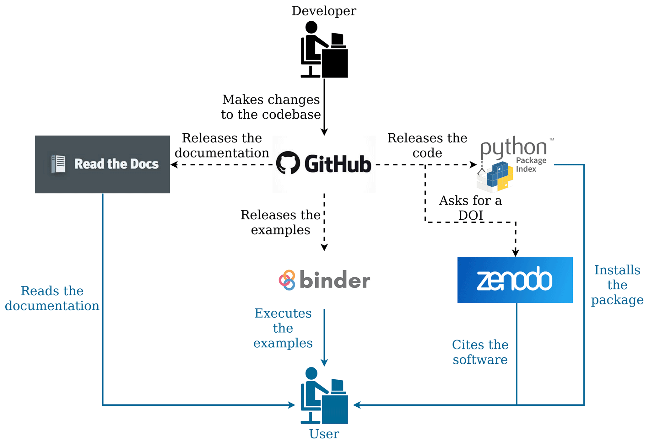
Figure 13 Organization of the SuperflexPy project, indicating the online software management tools used to develop the source code and documentation, release product versions with associated DOIs, and provide general open access to all project components. Typical workflow paths for users and developers are shown, respectively, in the blue and black lines and font. Dashed lines represent automated workflows.

5.1.4 Possibility of extension and customization

Most frameworks have open-source code and permissive licenses, making it possible to modify and extend their code base. Within this category, some frameworks are specifically intended to be customized (e.g., implementing new functionalities) as part of their regular usage without an expectation of “developer-level” skills (e.g., ECHSE). Other frameworks do not envisage customization in their primary scope but can still be modified by modelers with appropriate programming expertise in consultation with available developer guides (e.g., RAVEN).

Some frameworks have not been released as open-source, and the only way to access their code base for customization and extension is by contacting their developers (e.g., SUPERFLEX-F90, PERSiST).

SuperflexPy is designed to facilitate extension and customization as part of its regular usage. New components can be created by extending or modifying existing components, as demonstrated in Sect. 3.2.

5.1.5 Computational efficiency

The computational efficiency of a model code, i.e., the time required to run a simulation, depends primarily on two aspects, namely the programming language and the numerical algorithms.

In terms of programming languages, most frameworks have been implemented in C, C$++$, or Fortran, which enable very fast computation. These implementations can be either purely single-language (e.g., FUSE, RAVEN) or wrapped within a scripting language to provide a more suitable interface (e.g., CMF). Amongst the considered existing frameworks, only MARRMoT is implemented entirely in an interpreted language (Matlab/Octave).

In terms of numerical algorithms, a wide range of options are available for solving differential equations. Broadly speaking, time stepping algorithms can be classified as implicit or explicit and may employ a fixed or an adaptive step size. The choice of algorithm and its settings brings tradeoffs between solution accuracy, algorithm complexity, and computational cost. In the context of model development and comparison, it is important to separate the specification of model equations from the choice of numerical solution and to use robust numerical methods to avoid spurious artifacts (e.g., Kavetski and Clark, 2010). The majority of frameworks implement this separation and provide a choice of built-in numerical algorithms.

SuperflexPy, while written entirely in Python (a nominally slow language), makes several implementation choices to reduce computational costs. These choices include the use of efficient numerical libraries (Sect. 4.4) and the solution of the elements in succession (DAG, Sect. 5.2). This solution of the elements “one at a time” enables the usage of robust solvers that operate on a single ODE at a time; in such cases, the root finder also operates on a single algebraic equation at a time, reducing the computational effort. The choice of numerical algorithm for individual elements is left to the user (Sect. 4.3). The (recommended) built-in approximators include the implicit Euler scheme with fixed step size, which offers stability and smoothness benefits valuable in parameter estimation contexts.

5.2 Current restrictions in model structure specification

As part of balancing the flexibility, ease of use, and computational performance of SuperflexPy, some restrictions have been imposed on the connectivity between model components.

The first restriction is that elements within a unit must form a directional acyclic graph (DAG), with no feedback loops from downstream to upstream elements (Sect. 2.1). This restriction enables the numerical solvers to proceed, at each time step, in a single pass from upstream to downstream elements and improves the computational performance of the framework. The restriction on internal model feedbacks is not expected to be overly limiting when developing conceptual hydrological models, where the fluxes from a given element typically depend only on the state in that element and not on downstream elements. In such systems, flows occur only in one direction, e.g., in model M4 the water flows from UR to FR but not vice versa. A counter-example where internal model feedbacks are required is given by the bidirectional interaction between surface water and groundwater in the hyporheic zone, where the exchange flux (or fluxes) depends on both states. Such interactions can still be modeled in SuperflexPy by introducing elements that embed feedbacks internally. For example, the hyporheic zone can be represented using a two-state reservoir with interacting states (e.g., Seibert et al., 2003). In other words, the SuperflexPy restriction on model feedbacks applies to interactions between elements but not to interactions within an element.

The second restriction, which also applies at the unit level, derives from the decision to define the DAG as a succession of layers (Sect. 5.1.1). This choice simplifies the model definition in typical use cases, when there are many elements with relatively few connections (i.e., the DAG is “sparse” rather than “dense”). However, the definition of a DAG as a succession of layers requires the elements to be connected directly one to the other, without skipping layers. Hence the need for transparent elements, which output the inputs they receive and are used to fill the gaps that arise when two or more parallel flow paths have a different number of elements. An example of such model configuration is given in Fig. 9, where a transparent element (labeled “lower_transparent”) is used to fill the gap in layer 7.

The third restriction is that the topology of a network must represent a tree where any given node can connect and transfer fluxes only to a single downstream node (Sect. 2.1). This restriction has a similar motivation to the restriction of a unit structure to a DAG and allows for a simple and efficient computational implementation, which starts from the headwater nodes and proceeds downstream one node at a time. Typical distributed conceptual models meet this restriction, for example as illustrated in Sect. 3.3. However, fully integrated distributed models, such as Parflow and Mike-She, do include mutual dependencies between spatial elements, e.g., leading to 2D or 3D groundwater flows. Such configurations are considered beyond the scope of conceptual distributed models and therefore are not currently supported in SuperflexPy.

5.3 Current usage and future developments

SuperflexPy is easy to install and run; it is written in pure Python and its dependencies are limited to the packages NumPy and Numba (Sect. 4.4). Installation can be done directly using the package installer for Python (pip) and do not require (additional) external libraries. We stress that SuperflexPy is not a wrapper of earlier SUPERFLEX-F90 code but offers a completely new implementation that is not constrained by choices taken in the earlier code versions.

SuperflexPy has already been used for research applications. Jansen et al. (2021) performed a “model mimicry” study where similarities and differences within the HBV family of models were investigated. SuperflexPy was used to construct a set of HBV-like models and compare them in terms of the behavior of individual model components, the impact of numerical implementation, and so forth. A list of publications using SuperflexPy is maintained on the documentation website.

In terms of future developments, we hope that SuperflexPy offers the broader hydrological community a versatile new tool for research work and practical applications. Further SuperflexPy developments are likely to follow from such work and collaborations, including (i) expansion of the library of model components beyond the ones here presented (as shown in the example in Sect. 3.2) and (ii) more fundamental developments in response to future model applications. It is important to highlight that SuperflexPy can be used to create and combine new model components, thereby enabling experimentation with new model structures and general conceptualizations. The framework, therefore, is not limited to components and structures taken from existing models – though such collections could be also produced. The SuperflexPy model library may grow as new users share their implementations with the community. In order to facilitate the use of SuperflexPy, its code is accessible on GitHub with license LGPL-3.0 and distributed using the Python package installer PyPI (see the code availability section at the end of this paper). The online documentation provides a guide for colleagues interested in contributing to the framework (Sect. 2.1 of the Supplement).

6 Summary and conclusions

SuperflexPy is a new Python flexible modeling framework for building conceptual catchment-scale hydrological models ranging from lumped to distributed configurations. SuperflexPy offers detailed control over each aspect of model configuration and caters to a wide range of typical conceptual model applications. In order to facilitate the model building process, the framework defines its components (building blocks) at four hierarchical levels, namely element, unit, node, and network. These components support conceptual model setups of increasing levels of complexity, including but not limited to a single element model (e.g., a reservoir), a typical lumped model (e.g., a collection of interconnected reservoirs), a semi-distributed model designed to provide prediction at a single outlet, and a semi-distributed model designed to provide predictions at internal sub-catchments. The construction of a model from components up to a given hierarchical level does not require specifying components at higher levels, which makes the model configuration effort proportional to the complexity of the application and reduces configuration and computational overheads. The framework supports multiple states and fluxes in each component, which facilitates future extension to applications where such functionality is needed.

SuperflexPy offers an open-source implementation of the SUPERFLEX principles (Fenicia et al., 2011) that builds on the collective experience of the authors and their colleagues in hydrological model design and application. The paper discusses the key design choices made in SuperflexPy, with an emphasis on the ease of use and interfacing, availability, amenability of extensions, and computational efficiency.

The use of the SuperflexPy framework is illustrated using two examples that represent typical tasks in conceptual hydrological modeling: the implementation of a lumped model to simulate an entire catchment and the implementation of a distributed model to simulate a system of multiple sub-catchments with spatially varying landscape characteristics. We hope the framework will contribute to ongoing efforts in the hydrological modeling community to develop more robust and representative models. The framework is open source, available with license LGPL-3.0 on GitHub.