ENSO-ASC 1.0.0: ENSO deep learning forecast model with a multivariate air–sea coupler

The El Niño–Southern Oscillation (ENSO) is an extremely complicated ocean–atmosphere coupling event, the development and decay of which are usually modulated by the energy interactions between multiple physical variables. In this paper, we design a multivariate air–sea coupler (ASC) based on the graph using features of multiple physical variables. On the basis of this coupler, an ENSO deep learning forecast model (named ENSO-ASC) is proposed, whose structure is adapted to the characteristics of the ENSO dynamics, including the encoder and decoder for capturing and restoring the multi-scale spatial–temporal correlations, and two attention weights for grasping the different air–sea coupling strengths on different start calendar months and varied effects of physical variables in ENSO amplitudes. In addition, two datasets modulated to the same resolutions are used to train the model. We firstly tune the model performance to optimal and compare it with the other state-of-the-art ENSO deep learning forecast models. Then, we evaluate the ENSO forecast skill from the contributions of different predictors, the effective lead time with different start calendar months, and the forecast spatial uncertainties, to further analyze the underlying ENSO mechanisms. Finally, we make ENSO predictions over the validation period from 2014 to 2020. Experiment results demonstrate that ENSO-ASC outperforms the other models. Sea surface temperature (SST) and zonal wind are two crucial predictors. The correlation skill of the Niño 3.4 index is over 0.78, 0.65, and 0.5 within the lead time of 6, 12, and 18 months respectively. From two heat map analyses, we also discover the common challenges in ENSO predictability, such as the forecasting skills declining faster when making forecasts through June–July–August and the forecast errors being more likely to show up in the western and central tropical Pacific Ocean in longer-term forecasts. ENSO-ASC can simulate ENSO with different strengths, and the forecasted SST and wind patterns reflect an obvious Bjerknes positive feedback mechanism. These results indicate the effectiveness and superiority of our model with the multivariate air–sea coupler in predicting ENSO and analyzing the underlying dynamic mechanisms in a sophisticated way.

1 Introduction

The El Niño–Southern Oscillation (ENSO) can induce global climate extremes and ecosystem impacts (Zhang et al., 2016), which are the dominant sources of interannual climate changes. The El Niño (La Niña) is the ocean phenomena of ENSO and is usually considered as the large-scale positive (negative) sea surface temperature (SST) anomalies in the tropical Pacific Ocean. The Niño 3 (Niño 4) index is the common indicator for ENSO research to measure the cold tongue (warm pool) variabilities, which is the averaged SST anomalies covering the Niño 3 (Niño 4) region (see Fig. 1). Besides these two indicators, the ONI (oceanic Niño index, 3-month running mean of SST anomalies in the Niño 3.4 region) has become the de facto standard to identify the occurrence of El Niño and La Niña events: if the ONIs of 5 consecutive months are over 0.5 ^∘C (below −0.5 ^∘C), El Niño (La Niña) occurs.

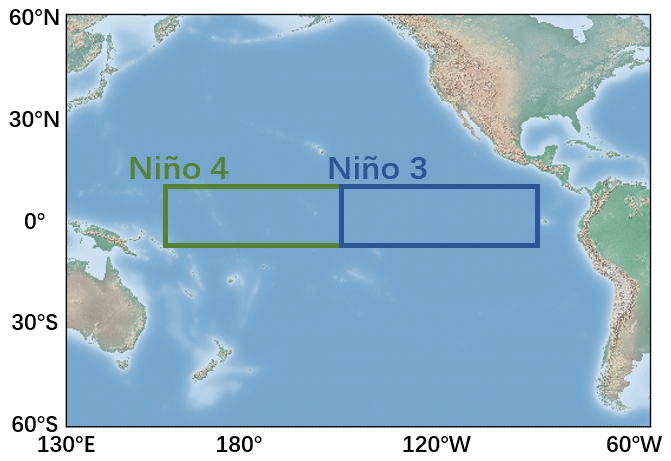
Figure 1 Regions most affected by ENSO events. The blue rectangle covers the Niño 3 region (5^∘ N–5^∘ S, 150^∘ W–90^∘ W), and the green rectangle covers the Niño 4 region (5^∘ N–5^∘ S, 160^∘ E–150^∘ W).

Conventional forecast approaches mainly rely on numerical climate models. However, it is worth noting that the model biases of traditional approach have always been a problem for accurate ENSO predictions (Xue et al., 2013). In addition, many other intrinsic factors also limit the ENSO predictability such as natural decadal variations in ENSO amplitudes. For example, predictability tends to be higher when the ENSO cycle is strong than when it is weak (Barnston et al., 2012; Balmaseda et al., 1995; McPhaden, 2012). Recently, due to deluges of multi-source real-world geoscience data starting to accumulate, e.g., remote sensing and buoy observation, meteorological researchers were inspired to build lightweight and convenient data-driven models at a low computational cost (Rolnick et al., 2019), which lead to a wave of formulating ENSO forecast with deep learning techniques, producing more skilful ENSO predictions (Ham et al., 2019).

In the field of deep learning, ENSO prediction is usually regarded as forecasting the future evolution tendency of SST and related Niño indexes directly, subsequently analyzing the associated sophisticated mechanisms, and measuring the intrinsic characteristics such as intensity and duration. Therefore, the simplest but most practical forecast manners can be divided into two categories intuitively: Niño index forecast and SST pattern forecast.

As for Niño index forecasting, many favorable neural networks have made accurate predictions 6, 9 and 12 months ahead. For instance, ensemble QESN (McDermott and Wikle, 2017), BAST-RNN (McDermott and Wikle, 2019) and LSTM (long short-term memory) (Broni-Bedaiko et al., 2019) are representative works. These studies demonstrate that the deep learning can well capture the nonlinear characteristics of non-stationary time series and attain outstanding regressions on Niño index.

Notwithstanding the successful attempts on the Niño index regression, there still exist many pitfalls in measuring ENSO forecast skills by only one single scalar. For example, the important spatial–temporal energy propagations and teleconnections cannot be described by the indexes. It may lead to the blind pursuit of the accuracy of a certain indicator while seriously hampering the grasp of underlying physical mechanisms. Therefore, many studies are suggestive of exploiting spatial–temporal dependencies and predicting the evolution of SST patterns. Ham et al. (2019) apply transfer learning (Yosinski et al., 2014) to historical simulations from CMIP5 (Coupled Model Intercomparison Project phase5, Bellenger et al., 2014) and reanalysis data with a CNN model to predict ENSO events, resulting in a robust and long-term forecast for up to 1.5 years, which outperforms the current numerical predictions. (Though the output of their model is still the Niño 3.4 index, they construct the model and make forecasts by absorbing the historical spatial–temporal features from variable patterns instead of previous index records, so we mark this study as SST pattern forecasts in this paper.) Mu et al. (2019) and He et al. (2019) built a ConvLSTM (Shi et al., 2015) model to capture the spatial–temporal dependencies of ENSO SST patterns over multiple time horizons and obtained better predictions. Zheng et al. (2020) constructed a purely satellite-data-driven deep learning model to forecast the evolutions of tropical instability wave, which is closely related to ENSO phenomena, and obtained accurate and efficient forecasts. These deep learning models tend to simulate the behaviors of numerical climate models, the inputs of which are historical geoscience data and the outputs of which are the forecasted SST patterns.

The reason for the great progress in these works is no accident. On the one hand, the deep learning models have much more complex structures and can mine the complicated features hidden in the samples more effectively, which allows them to be substantially more expressive with blending the non-stationarity in temporal and the multi-scale teleconnections in spatial. On the other hand, it is very convenient to migrate deep learning computer vision technologies to ENSO forecasting due to the nature analogy between the format of image/video frame data and meteorological time-series grid data, which offers promises for extracting spatial–temporal mechanisms of ENSO via advanced deep learning techniques. Therefore, the data-driven deep learning can be a reliable alternative to traditional numerical models and a powerful tool for the ENSO forecasting.

However, there are still some obstacles in the deep learning modeling process for ENSO forecasting. Very often, most existing models are confined to limited or even single input predictors, such as only using historical SST (and wind) data as the model input. Meanwhile, the climate deep learning models are rarely adaptively customized to the specific physical mechanisms of ENSO. These situations lead to poor interpretability and low confidence of ENSO-related deep learning models. ENSO is an extremely complicated ocean–atmosphere coupling event, and the development and decay phases are closely associated with some crucial dynamic mechanisms and Walker circulation (Bayr et al., 2020), whose status have great impacts. Walker circulation is usually modulated by multi-physical variables (such as SST, wind, precipitation, etc.), and there are always coupling interactions between different variables. More specifically, the varieties of the Walker circulation have strong temporal-lag effects on ENSO (“memory effects”). The position of the ascending branch is also a very important climatic condition for the occurrence of El Niño. Such a priori ENSO knowledge has not been effectively used in deep learning model.

Therefore, in order to further improve the ENSO prediction skill, there is an essential principle that should be reflected in climate deep learning models: subjectively incorporating the a priori ENSO knowledge into the deep learning formalization and deriving hand-crafted features to make predictions.

In this paper, according to the important synergies of multiple variables in crucial ENSO dynamic mechanisms and Walker circulation, we select six indispensable variables (SST, u wind, v wind, rain, cloud, and vapor) that are induced from ENSO-related key processes to build a multivariate air–sea coupler (ASC) based on a graph mathematically, which emphasizes the energy exchange between multiple variables. We then leverage this coupler to build up the ENSO deep learning forecast model, named ENSO-ASC, with an encoder–coupler–decoder structure to extract the multi-scale spatial–temporal features of multiple physical variables. Two attention weights are also proposed to grasp the different air–sea coupling strengths on different start calendar months and varied effects of these variables. A loss function combining MSE (mean squared error) and MAE (mean absolute error) is used to guide the model training precisely, and SSIM (structural similarity) (Wang et al., 2004) and PSNR (peak signal-to-noise ratio) are used as metrics to evaluate the spatial consistency of the forecasted patterns.

Two datasets are applied for model training to ensure that the systematic forecast errors are fully corrected after tuning by the higher quality dataset: we first train the ENSO-ASC on the numerous reanalysis samples from January 1850 to December 2015 and subsequently on the high-quality remote sensing samples from December 1997 to December 2012 for fine-tuning. This procedure is also known as transfer learning. These two datasets are modulated to the same resolution. The validation period is from January 2014 to August 2020 in the remote sensing dataset. The gap between the fine-tuning set and validation set is used to remove the possible influence of oceanic memory (Ham et al., 2019).

This is the first time that a multivariate air–sea coupler has been designed that considers energy interactions. We evaluate the ENSO-ASC from three aspects: firstly, we evaluate the model performance from the perspective of model structure, including the input sequence length, the benefits of transfer learning, multivariate air–sea coupler, and the attention weights, and tune the model structure to optimal. Then, we analyze the ENSO forecast skill of the ENSO-ASC from the meteorological aspects, including the contributions of different input physical variables, the effectiveness of forecast lead time, the forecast skill changes with different start calendar months, and the forecast spatial uncertainties. Subsequently, we make the real-world ENSO simulations during the validation period by tracing the evolutions of multiple physical variables. From the experiment results, ENSO-ASC performs better in both SSIM and PSNR of the forecasted SST patterns, which effectively raises the upper limitation of ENSO forecasts. The forecasted ENSO events are more consistent with real-world observations and the related Niño indexes have higher correlations with observations than traditional methods and current state-of-the-art deep learning models, which is over $\mathrm{0.78}/\mathrm{0.65}/\mathrm{0.5}$ within the lead time of $\mathrm{6}/\mathrm{12}/\mathrm{18}$ months for Niño 3.4 index. SST and zonal wind are two crucial predictors, which can be considered as the major triggers of ENSO. A temporal heat map analysis illustrates that the ENSO forecasting skills decline faster when making forecasts through June–July–August, and a spatial heat map analysis shows that the forecast errors are more likely to show up over the central tropical Pacific Ocean in longer-term forecasts. Meanwhile, in the validation period from 2014 to 2020, the multivariate air–sea coupler can capture the latent ENSO dynamical mechanisms and provide multivariate evolution simulations with a high degree of physical consistency: The positive SST anomalies first show up over the eastern equatorial Pacific with the westerly wind anomalies in the western and central tropical Pacific Ocean (vice versa in the La Niña events), which induces Bjerknes positive feedback mechanism. It is worth noting that for the simulation of the 2015–2016 super El Niño, ENSO-ASC captures its strong evolutions of SST anomalies over the northeast subtropical Pacific in the peak phase and successfully predicts its very-high-intensity and very-long-duration, while many dynamic or statistical models fail. At the same time, ENSO-ASC can also reduce false alarm rate such as in 2014. From the mathematical expression, the multivariate air–sea coupler captures the spatial–temporal multi-scale oscillations of the Walker circulation and performs the ocean–atmosphere energy exchange simultaneously, which tries to avoid the interval flux exchange in geoscience fluid programming of traditional numerical climate models. In conclusion, the graph-based multivariate air–sea coupler not only exhibits effectiveness and superiority to predict sophisticated climate phenomena, but is also a promising tool for exploiting the underlying dynamic mechanisms in the future.

The remainder of this paper is organized as follows. Section 2 introduces the proposed multivariate air–sea coupler. Section 3 describes the ENSO deep learning forecast model with the coupler (ENSO-ASC) in detail. Section 4 illustrates the datasets, experiment schemas and result analyses. Finally, Sect. 5 offers further discussions and summarizes the paper.

2 Multivariate air–sea coupler based on graph

ENSO is the most dominant phenomenon of air–sea coupling over the equatorial Pacific, and many complex dynamical mechanisms modulate the ENSO amplitudes. Bjerknes positive feedback (Bjerknes, 1969) is one of the most significant effects, the processes of which are highly related to the status of the Walker circulation. There are energy interactions between the multiple physical variables influenced by Walker circulation every moment, and the ENSO-related SST varieties are greatly affected by such air–sea coupling activities (Gao and Zhang, 2017; Lau et al., 1989; Lau et al., 1996).

Many atmospheric and oceanic anomalies are known as triggers of ENSO events, which establish the Bjerknes positive feedback. The warming SST anomalies propagate to the central and eastern equatorial Pacific gradually. As SST gradually rises, it is virtually impossible for the equatorial Pacific to enter a never-ending warm state. Therefore, some negative feedback will cause turnabouts from warm phases to cold phases (Wang et al., 2017). These negative feedback mechanisms all emphasize air–sea interactions. For example, westerly wind anomalies in the central tropical Pacific Ocean induce the upwelling Rossby and downwelling Kevin oceanic waves, both of which propagate and reflect on the continental boundary and then tend to push the warm pool back to its original position in the western Pacific. From the perspective of ENSO life cycle, atmospheric and oceanic variables play crucial roles together.

Meanwhile, during the development and decay phases of ENSO, there also exist nonlinear interactions between atmospheric and oceanic variables. Wind anomalies are the most obvious and direct response of the ENSO-driven large-scale oceanic varieties, and they will change the ocean–atmosphere heat transmissions (Cheng et al., 2019). Once the ocean status changes, the thermal energy contained in the sea will escalate or dissipate into the air, hindering or promoting the precipitation and surface humidity over the equatorial Pacific. These changes also give feedback on the ENSO.

Meteorological researchers have already identified the key physical processes in ENSO in recent years. If such knowledge can be incorporated into ENSO deep learning forecast modeling subjectively, breaking away from the current limitation of using single predictors, the accuracy of ENSO prediction will promise breakthroughs. In this paper, we choose six ENSO-related indispensable variables from two different multivariate datasets as shown in Table 1, which all have strong correlations within the evolution of ENSO events according to Bjerknes positive feedback and other dynamical processes. Furthermore, in order to comprehensively represent the coupling interactions, a multivariate air–sea coupler coupler(G) is designed to simulate their synergies with an undirected graph $G=(V,A)$ as shown in Fig. 2, where $V=(f_{v_{\mathrm{1}}}{f}_{v_{\mathrm{2}}},\mathrm{\dots },f_{v_N})$ represents the vertices of the graph and $f_{v_i}$ is the feature of every physical variable v_i ($i=\mathrm{1},\mathrm{2},\mathrm{\dots },N)$. $\mathbf{A}\in R^{N\times N}$ is the pre-designed adjacency matrix, where $A_{i,j}=\mathrm{1}$ ($A_{i,j}=\mathrm{0})$ represents the existing (non-existent) energy interactions between the connected variables v_i and v_j. The variables exchange energies simultaneously every moment, and the directions of edges in this graph can be neglected because the energy interactions are two-way (transfer and feedback).

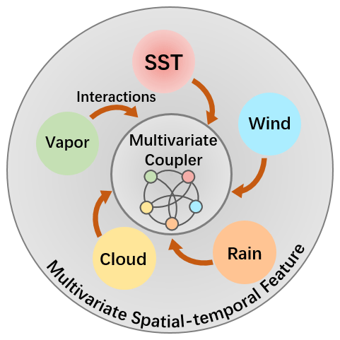
Figure 2 A description of our proposed multivariate air–sea coupler, which utilizes the spatial–temporal features of multiple physical variables to simulate the energy exchanging simultaneously.

Here, V in G is not the physical variable on a single grid point, but the features of the entire variable pattern. The reason lies in the following: on the one hand, the coupler will pay more attention to the global and local spatial–temporal correlations in the variable fields of ENSO rather than the variations on an isolated grid. On the other hand, the coupler will provide a higher computational efficiency and consume a lower calculation resource for ENSO forecasting. Improvements to the couplers, such as designing individual graph for smaller-scale regions and even a single grid, are future considerations.

3 ENSO-ASC: ENSO deep learning forecast model with the multivariate air–sea coupler

Inspired by previous ENSO deep learning forecast models, we can define the ENSO forecast as a multivariate spatial–temporal sequence forecast problem as illustrated in Eq. (1),

$$\begin{array}{}\text{(1)}& \widehat{s}=F_{\mathit{\theta }}\left(s^{\mathrm{scm}}\right),\mathit{\left\{}\text{sst,uwind,vwind,rain,cloud,vapor}\mathit{\right\}}\subseteq s^{\mathrm{scm}},\end{array}$$

where $s^{\mathrm{scm}}\in R^{N\times M}$ is N multivariate observations in historical M months (N=6), and $\widehat{s}\in R^{N\times H}$ is the prediction result for future H months (H can be also treated as forecast lead time). scm$\in \mathit{\{}\text{Jan},\text{Feb},\mathrm{\dots },\text{Dec}\mathit{\}}$ (start calendar month) represents the last month in the input series s^scm. F_θ represents the forecast system (θ denotes the trainable parameters in the system).

In order to incorporate the multivariate coupler, we break down the conventional formulation and redefine the multivariate ENSO forecast model as the encoder–coupler–decoder structure shown as in Eqs. (2) to (4),

$$\begin{array}{}\text{(2)}& {\displaystyle }\text{encoder:}{f}_{v_i}={\mathrm{encoder}}_i\left(s_i^{scm}\right),\text{(3)}& {\displaystyle }\begin{array}{rl}\text{coupler:}{f}_c& =\text{coupler}\left(G\right)\\ & =\text{coupler}\left(\right(f_{v_{\mathrm{1}}}\mathrm{|}\mathrm{|}{f}_{v_{\mathrm{2}}}\mathrm{|}\mathrm{|}\mathrm{\dots }\mathrm{|}\mathrm{|}{f}_{v_N}),A),\end{array}\text{(4)}& {\displaystyle }\text{decoder:}{\widehat{s}}_i={\mathrm{decoder}}_i\left(f_{v_i}\mathrm{|}\mathrm{|}{f}_{c_i}\right),\end{array}$$

where the $s_i^{\mathrm{scm}}(i=\mathrm{1},\mathrm{2},\mathrm{\dots },N)$ represents the individual physical data and $f_{v_i}$ represents the corresponding extracted features by respective encoders. The coupler (•) simulates the latent multivariate interactions on the physical features and the pre-designed interaction graph A, where the operator || represents the concatenation of features of different physical variables. Then the respective decoders will restore the physical features end-to-end by the coupled multivariate features $f_{c_i}$ and original physical features $f_{v_i}$, the concatenation of which can be regarded as skip-layer connections. These connections can propagate the low-level feature to high levels of the model directly, preserving the raw information and accelerating feature transfers to some extent. The sub-modules encoder_i(•), coupler(•), and decoder_i(•) form the ENSO-ASC together.

As mentioned before, the strength of the multivariate coupling and the effects of multivariate temporal memories in ENSO are changing with different input sequence length M and forecast start calendar month scm. In order to grasp such effects on forecasts, we design two self-supervised attention weights, $\mathit{\alpha }=(a_{\mathrm{1}},a_{\mathrm{2}},\mathrm{\dots },a_M)$ and $\mathit{\beta }=(b_{\mathrm{1}},b_{\mathrm{2}},\mathrm{\dots },b_N)$, in the encoder and coupler respectively to capture the dynamic time-series non-stationarity and re-weight the multivariate contributions. The final formulation of the forecast model can be written as shown in Eqs. (5) to (7) and in Fig. 3, where ∘ represents the element-wise multiplication.

$$\begin{array}{}\text{(5)}& {\displaystyle }\text{encoder:}{f}_{v_i}=\mathit{\alpha }\circ {\text{encoder}}_i\left(s_i^{scm}\right)\text{(6)}& {\displaystyle }\begin{array}{rl}\text{coupler:}{f}_{\mathrm{c}}& =\text{coupler}\left(\mathit{\beta }\circ G\right)\\ & =\text{coupler}\left(\right(b_{\mathrm{1}}{f}_{v_{\mathrm{1}}}\mathrm{|}\mathrm{|}{b}_{\mathrm{2}}{f}_{v_{\mathrm{2}}}\mathrm{|}\mathrm{|}\mathrm{\dots }\mathrm{|}\mathrm{|}{b}_N{f}_{v_N}),A)\end{array}\text{(7)}& {\displaystyle }\text{decoder:}{\widehat{s}}_i={\mathrm{decoder}}_i\left(f_{v_i}\mathrm{|}\mathrm{|}{f}_{c_i}\right)\end{array}$$

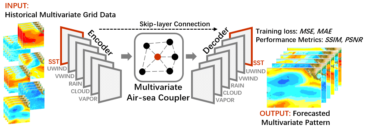
Figure 3 The structure of ENSO-ASC. There are six encoders for the chosen variables to extract spatial–temporal information and a multivariate air–sea coupler to simulate interactions. After interactions, we design six decoders to restore the major variable SST and other variables. The training loss and performance metrics are also displayed.

In addition, there are basically two forecast strategies for ENSO prediction: direct multi-step (DMS) and iterated multi-step (IMS) (Chevillon, 2007). The former means predicting the future Hth-month multivariate pattern directly, and the latter means utilizing the forecast output result as the input for future iterated predictions. Figure 4 displays the differences between DMS and IMS. In general, DMS is often unstable and more difficult to train for a deep learning model (Shi and Yeung, 2018). Therefore, we choose IMS to handle chaos data and provide more accuracy predictions, that is, forecasting the next 1-month (H=1) multivariate data in the model, and then using this output as model input to continuously predict the future evolutions. We also design a combined loss function to train our model and use two spatial metrics to evaluate the forecast results. The intentions and detailed implementations of every part in the model are interpreted as the following sections.

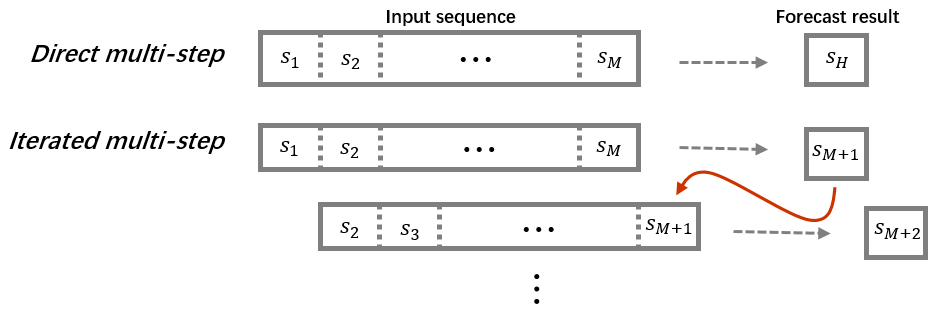
Figure 4 Two common ways in sequence prediction for ENSO forecasts: direct multi-step (DMS) and iterated multi-step (IMS).

3.1 Encoder: stacked ConvLSTM layers for extracting spatial–temporal features

The ENSO evolution has a strong correlation with historical atmospheric and oceanic memory (W. Zhang et al., 2019). An ENSO deep learning forecast model should be able to simultaneously extract the long-term spatial–temporal features from multivariate geoscience grid data and effectively mine the complicated nonlinearity hidden in the data. Stacked ConvLSTM layers are constructed as the skeleton of the encoder (see orange arrows in Fig. 5) for each chosen physical variable individually.

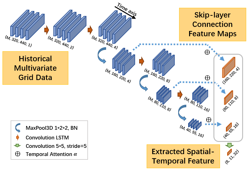
Figure 5 A detailed structure for encoder: a stacked ConvLSTM encoder for extracting spatial–temporal features simultaneously. There is also temporal attention weight for skip-layer connections in the grey box.

In order to capture the multi-scale spatial teleconnections in ENSO amplitudes, we set a 3D max-pool layer between two ConvLSTM layers respectively (as blue arrows in Fig. 5), the stride of which on the time axis is set to 1 to retain the sequence length M. Considering these obtained multi-scale spatial features after every 3D max-pool layers, we design the skip-layer connections shown in the grey box in Fig. 5. These layers propagate and cascade the raw features of the same variable from its encoder (lower levels) to its decoder (higher levels) directly (See Fig. 9) like dense connections (Huang et al., 2017). Such a structure can preserve more details at multi-scale spatial teleconnections and also solve the problem of gradient disappearance. In addition, we design the encoders and decoders to be symmetric, ensuring that the feature maps in these connections have the same shape.

Since we set H=1 as the IMS forecast strategy, the feature maps on the encoder all have a time axis, which the decoders do not have. The memory effects on the forecast are mutative with different input sequence lengths and forecast start calendar months; if we propagate all time steps' feature maps from the encoder to the coupler and the decoder, it is too redundant and even causes over-averaged forecast results, which hinders the descriptions of the special seasonal amplitudes. Therefore, before the skip-layer connections, we first determine the attention weights to dynamically fuse multiple time steps' feature maps in the encoder, which can capture the seasonal periodicity hidden in the physical variables and is also called temporal attention weight α (shown as ⊕ symbols in Fig. 5).

After obtaining sequential feature maps $T=\left[t_{\mathrm{1}},t_{\mathrm{2}},\mathrm{\dots },t_m\right]m=\mathrm{1},\mathrm{2},\mathrm{\dots },M$ from each 3D max-pool layer, we first flatten every time step feature map $t_m\in R^{w\times h\times c}$ by the width w, height h, and channel c as $t_m^{\prime }\in R^{\mathrm{1}\times (w\times h\times c)}$ and then cascade them together along the time axis as $T^{\prime }=\left[t_{\mathrm{1}}^{\prime },t_{\mathrm{2}}^{\prime },\mathrm{\dots },t_m^{\prime }\right]m=\mathrm{1},\mathrm{2},\mathrm{\dots },M$, where $T^{\prime }\in R^{M\times (w\times h\times c)}$. We apply Eq. (8) on T^′ to determine the self-supervised attentive weight α∈R^M for each time step's feature map t_m.

$$\begin{array}{}\text{(8)}& \mathit{\alpha }=\text{softmax}({\mathbf{W}}_{\mathit{\alpha }\mathrm{t}}\tanh \left({\mathbf{W}}_{\mathrm{t}}{T}^{\prime }+b_{\mathrm{t}}\right)+b_{\mathit{\alpha }t}),\end{array}$$

where ${\mathbf{W}}_{\mathrm{t}}\in R^{d_{\mathrm{1}}\times M}$ and ${\mathbf{W}}_{\mathit{\alpha }\mathrm{t}}\in R^{d_{\mathrm{1}}}$ are transformation matrices, d₁ is a hyper parameter, and $b_{\mathrm{t}}\in R^{d_{\mathrm{1}}}$ and b_αt∈R are biases. Every dimension in α represents the contribution to the forecast of corresponding time step, and we use Eq. (9) to fuse the original feature $T=\left[t_{\mathrm{1}},t_{\mathrm{2}},\mathrm{\dots },t_m\right]m=\mathrm{1},\mathrm{2},\mathrm{\dots },M$.

$$\begin{array}{}\text{(9)}& \stackrel{\mathrm{̃}}{T}=h\left(\mathit{\alpha },T\right)=\sum _{m=\mathrm{1}}^M({\mathit{\alpha }}_m\circ t_m),\end{array}$$

where $\stackrel{\mathrm{̃}}{T}$ is the aggregated feature map for skip-layer connections, and function h(•) represents the summary of element-wise multiplication.

The feature map sizes are described in Fig. 5 in detail. The sizes of ConvLSTM kernels are all 3×3 and the channel sizes are $[\mathrm{2},\mathrm{4},\mathrm{8},\mathrm{16}]$ during forward propagation, where the changes between adjacent layers are smooth and small. The final output (with size of $\mathrm{16}\times \mathrm{40}\times \mathrm{55})$ of the encoder is generated by a convolution layer of $\mathrm{32}\times \mathrm{5}\times \mathrm{5}$ with stride 5 and output a feature map with size of $\mathrm{8}\times \mathrm{11}\times \mathrm{32}$, which is used to filter the noise derived by such the deep-layer structure.

3.2 Multivariate air–sea coupler: learning multivariate synergies via graph convolution

From the perspective of ENSO dynamics, the occurrences of ENSO are accompanied by energy interactions. Based on our formalization and chosen physical variables, we define the corresponding adjacency matrix $\mathbf{A}\in R^{\mathrm{6}\times \mathrm{6}}$ and degree matrix $\mathbf{D}\in R^{\mathrm{6}\times \mathrm{6}}$ (the diagonal matrix, the value on the diagonal indicates the number of other vertices connected to this vertices) as in Eq. (10), which means all physical variables have coupling interactions with each other (fully connected).

$$\begin{array}{}\text{(10)}& \mathbf{A}=\left[\begin{array}{ccc}\mathrm{1}& \mathrm{\cdots }& \mathrm{1}\\ \mathrm{⋮}& \mathrm{\ddots }& \mathrm{⋮}\\ \mathrm{1}& \mathrm{\cdots }& \mathrm{1}\end{array}\right]\mathbf{D}=\left[\begin{array}{ccc}\mathrm{6}& \mathrm{\cdots }& \mathrm{0}\\ \mathrm{⋮}& \mathrm{\ddots }& \mathrm{⋮}\\ \mathrm{0}& \mathrm{\cdots }& \mathrm{6}\end{array}\right]\end{array}$$

In practical implementation mathematically, we use a graph Laplacian matrix L to normalize the energy flow of original adjacency matrix A as in Eq. (11), where I_n is an identity matrix with the order n×n. L can be considered as the directions in which the excess unstable energy will propagate to other variables when the entire system is perturbed (such as external wind forcing).

$$\begin{array}{}\text{(11)}& \mathbf{L}=I_n-{\mathbf{D}}^{-\frac{\mathrm{1}}{\mathrm{2}}}{\mathbf{AD}}^{-\frac{\mathrm{1}}{\mathrm{2}}}\end{array}$$

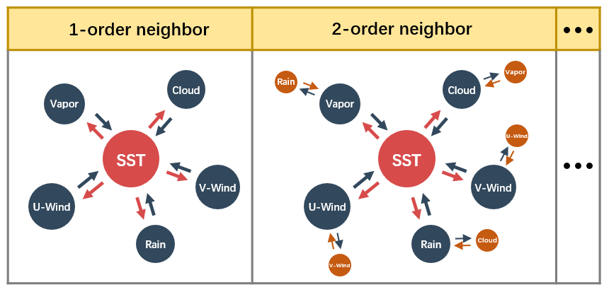
Figure 6 Multivariate coupling interactions within K-order neighbors (taking SST as the center).

Meanwhile, the interactions between ENSO-related variables are cascaded, which means that the effects between physical variables are multi-order as depicted in Fig. 6. For example, the precipitation anomalies affect the wind anomalies, which in turn affect the evolutions of SST, as depicted in Fig. 6 (right). According to the properties of the Laplacian matrix, L^K is employed to determine the cascaded interactions between K-order neighbors. So, if we consider K-order effects, the whole process is defined by Eq. (12),

$$\begin{array}{}\text{(12)}& P^{(l+\mathrm{1})}=\mathit{\sigma }\left(\sum _{k=\mathrm{1}}^K{\mathrm{\Theta }}^{\left(k\right)}{L}^K{P}^{\left(l\right)}\right),\end{array}$$

where Θ^(k) represents the latent trainable multivariate interactions. K represents the truncated order of effects concerned. P^(l) represents the input features before coupling interactions and P^(l+1) represents the coupled features. Each row in both P^(l) and P^(l+1) represents the same variables. Activation function σ increases the nonlinearity. Figure 7 illustrates the above process mathematically, which is named as the K-order graph convolution layer.

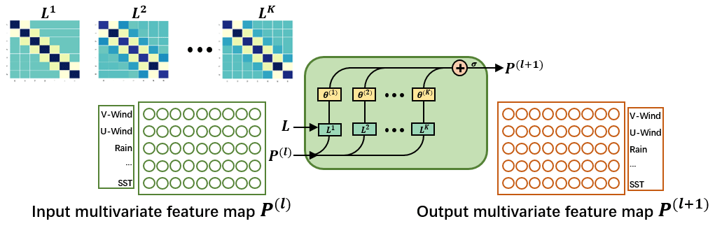
Figure 7 K-order graph convolution layer. K is the truncated order and L^K represents the interactions between K-order neighbors. Each row in p^(l) and p^(l+1) represents features of different physical variables, and their positions are not changed during forward propagation.

The K-order graph convolution network (GCN) in Eq. (12) is actually the higher-order extension of original GCN (Bruna et al., 2013). Furthermore, we use Chebyshev polynomial $T_K\left(\stackrel{\mathrm{̃}}{L}\right)$ to approximate the higher-order polynomial $\left[L^{\mathrm{1}},L^{\mathrm{2}},\mathrm{\dots },L^K\right]k=\mathrm{1},\mathrm{2},\mathrm{\dots },K$ to accelerate calculation, where $\stackrel{\mathrm{̃}}{L}=\mathrm{2}L/{\mathit{\lambda }}_{max}-I_n$ scales L within $[-\mathrm{1},\mathrm{1}]$ to satisfy the Chebyshev polynomial and λ_max is the maximum Eigen value of L (Hammond et al., 2011; Defferrard et al., 2016). This approximation accelerates the calculation of the K-order GCN by reducing the computational complexity from O(n²) to O(K|ε|) (|ε| is the edge count in the graph). Based on such neural structure, we construct the multivariate air–sea coupler (ASC) to learn synergies related to ENSO as in Fig. 8.

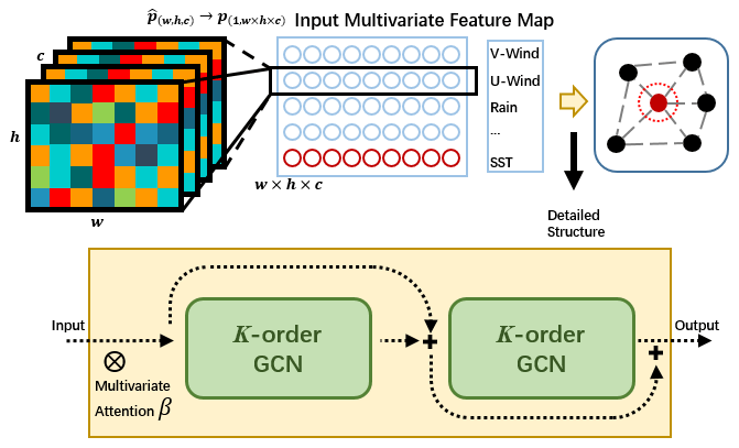
Figure 8 A detailed structure for multivariate air–sea coupler between encoder and decoder: pre-processes for input (upper row), and dual-layer structure for residual learning (lower row). There is also a multivariate attention weight in the coupler.

After obtaining the spatial–temporal features (Such as the colored feature maps in Fig. 8) from multivariate encoders respectively, we first flatten and cascade them as P^(l) like the blue box in Fig. 8. As mentioned above, each row of P^(l) represents different variables. P^(l) is marked as multivariate feature map and acts as the input of the coupler. The coupler is designed as a dual-layer summation structure like the yellow box in Fig. 8. The input for the second layer is the sum of the input and the output of the first layer, and the output of the second layer is determined by the weighted fusion of the outputs of these two layers in the manner designed by Chen et al. (2019), which is the residual learning to enhance the generalization ability of the network (He et al., 2016).

Because the variables contribute differently to the ENSO forecast, especially in different start calendar months, we propose the multivariate self-supervised attention weight for determining the effects for the input physical variables as ⊗ symbols in Fig. 8. Before P^(l) passes into the multivariate coupler, the weight β∈R^N for each variable is determined by Eq. (13).

$$\begin{array}{}\text{(13)}& \mathit{\beta }=\text{softmax}\left({\mathbf{W}}_{\mathit{\beta }p}\tanh \left({\mathbf{W}}_p{P}^{\left(l\right)}+b_p\right)+b_{\mathit{\beta }p}\right),\end{array}$$

where ${\mathbf{W}}_p\in R^{d_{\mathrm{2}}\times N}$ and ${\mathbf{W}}_{\mathit{\beta }p}\in R^{d_{\mathrm{2}}}$ are transformation matrices, d₂ is a hyper parameter, and $b_p\in R^{d_{\mathrm{2}}}$ and b_βp∈R are biases. Then we use Eq. (14) to calculate the modulated multi-physical variable feature map, where g(•) represents the element-wise multiplication.

$$\begin{array}{}\text{(14)}& P^{\left(l\right)}=g\left(\mathit{\beta },P^{\left(l\right)}\right)=\mathit{\beta }⊡P^{\left(l\right)}\end{array}$$

In the multivariate air–sea coupler, the corresponding locations of physical variables on the input feature map and output feature map are fixed. For example, if we set the SST feature in the last row of the input multivariate feature map of the coupler, the SST feature will be in the last row of the output multivariate feature map as shown in Fig. 7 and will be propagated to the decoder for pattern prediction later.

3.3 Decoder: end-to-end learning to restore the forecasted multivariate patterns

ENSO evolution is considered as a hydrodynamic process. Meteorologists usually use linear methods, such as empirical orthogonal function (EOF) or singular value decomposition (SVD) methods to extract features and then analyze the potential characteristics and predict the future evolution of ENSO. In these methods, complex dynamical processes are usually simplified to facilitate calculations while unknown detailed processes are not comprehensively revealed or even neglected, which leads to low prediction accuracy. Therefore, we use the end-to-end learning to restore the evolutions of multi-physical variable patterns. The multi-scale spatial–temporal correlations should be also considered in this process, so the decoder consists of stacked transform-convolution layers and up-sampling layers.

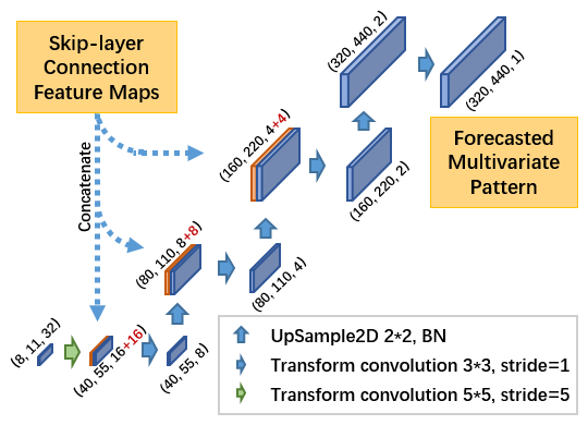
Figure 9 A detailed structure for decoder, skip-layer connections from encoder for helping end-to-end learning to restore the forecasted patterns at different spatial scales.

From the output feature map of the multivariate air–sea coupler, we pick up the corresponding row (taking SST as an example) as P_SST (such as the red row and red circle in Fig. 8) and reshape it into original shape $P_{\mathrm{SST}}^{\prime }\in R^{w\times h\times c}$. Then $P_{\mathrm{SST}}^{\prime }$ is gradually amplified and restored in the decoder by the stacked transform–convolution layers and up-sampling layers (see Fig. 9). Skip-layer feature maps from the encoder are cascaded with corresponding layers with the same shape. The sizes of convolution kernels are all 3×3 which is the same with that in the encoder, and the channel sizes are $[\mathrm{16},\mathrm{8},\mathrm{4},\mathrm{2},\mathrm{1}]$ to shrink the channel size gradually during forward propagation.

3.4 Loss functions for model training

Our goal is to predict the evolutions of multiple physical variables (marked as $\widehat{s})$ as accurately as possible compared with the real-world observation s. Therefore, we combine two different measurements together as the loss function l in Eq. (15) to ensure the result precision of multivariate patterns grid by grid,

$$\begin{array}{}\text{(15)}& \left\{\begin{array}{ll}& \text{MSE}=\frac{\mathrm{1}}{N\mathrm{\Omega }}{\sum }_N{\sum }_{\mathrm{\Omega }}{\left({\widehat{s}}_{i,j}-s_{i,j}\right)}^{\mathrm{2}}\\ & \text{MAE}=\frac{\mathrm{1}}{N\mathrm{\Omega }}{\sum }_N{\sum }_{\mathrm{\Omega }}\left|{\widehat{s}}_{i,j}-s_{i,j}\right|\\ & l=\mathrm{MSE}+\mathrm{MAE}\end{array},\left(i,j\right)\in \mathrm{\Omega }\right.,\end{array}$$

where N is the number of variables and Ω represents the number of grid points for every physical pattern; (i,j) represent different latitude and longitude; l is the sum of MSE and MAE, where MSE is used to preserve the smoothness of the forecasted patterns; and MAE is used to retain the peak distribution of all grid points.

3.5 Metrics to evaluate the forecast results

According to the loss function, the calculation processes in Eq. (15) mainly focus on the comparisons of a single grid in fields. However, the detailed spatial distributions of every physical variable, such as the location of the max value region for SST and wind anomalies, are more important in the ENSO forecast. Therefore, we use the following two common spatial metrics for the forecasted patterns to evaluate the ENSO forecast skill: PSNR and SSIM as in Eqs. (16) and (17).

$$\begin{array}{}\text{(16)}& {\displaystyle }\text{PSNR}=\mathrm{10}\times {\log }_{\mathrm{10}}\left({\displaystyle \frac{{\mathrm{MAX}}^{\mathrm{2}}}{\mathrm{MSE}}}\right)\text{(17)}& {\displaystyle }\left\{\begin{array}{ll}& \text{luminance}=\frac{\mathrm{2}{\mathit{\mu }}_{\widehat{s}}^{\mathrm{2}}{\mathit{\mu }}_{\mathrm{s}}^{\mathrm{2}}+c_{\mathrm{1}}}{{\mathit{\mu }}_{\widehat{s}}^{\mathrm{2}}+{\mathit{\mu }}_{\mathrm{s}}^{\mathrm{2}}+c_{\mathrm{1}}}\\ & \text{contrast}=\frac{\mathrm{2}{\mathit{\sigma }}_{\widehat{s}s}+c_{\mathrm{2}}}{{\mathit{\sigma }}_{\widehat{s}}^{\mathrm{2}}+{\mathit{\sigma }}_{\mathrm{s}}^{\mathrm{2}}+c_{\mathrm{2}}}\\ & \text{structure}=\frac{{\mathit{\sigma }}_{\widehat{s}s}+c_{\mathrm{3}}}{{\mathit{\sigma }}_{\widehat{s}}{\mathit{\sigma }}_{\mathrm{s}}+c_{\mathrm{3}}}\\ & \text{SSIM}={\text{luminance}}^a\cdot {\text{contrast}}^b\cdot {\text{structure}}^c\end{array}\right.\end{array}$$

In PSNR, MAX is the maximum among all grids. In ENSO-ASC, before the historical multivariate data are propagated into the model, we first normalize them in the range [0,1] as in Eq. (18). Therefore, MAX is set to 1.

$$\begin{array}{}\text{(18)}& x^{\ast }={\displaystyle \frac{x-x_{min}}{x_{max}-x_{min}}}\end{array}$$

SSIM is a combined metric of luminance, contrast, and structure between two patterns. ${\mathit{\mu }}_{\widehat{s}}$ (μ_s) is the average for $\widehat{s}$ (s), and ${\mathit{\sigma }}_{\widehat{s}}$ (σ_s) is the corresponding standard deviations. ${\mathit{\sigma }}_{\widehat{s}s}$ represents the covariance, and $a=b=c=\mathrm{1}$ for fair measurement of every ingredient of SSIM. c₁, c₂, and c₃ are all trivial values for preventing the denominator from being 0.

Besides these two metrics, the correlations between the calculated and the official Niño indexes will be also used to evaluate forecast skills.

4 Experiment results and analysis

4.1 Dataset description

After the deep learning model structure is determined, the quantity and quality of the training dataset affect the forecast performance decisively. As the improvement of observation ability, there are growing ways to provide multiple real-world observations, such as remote sensing satellites and buoy observation, which is more and more beneficial to building our ENSO forecast model. However, one of the biggest limitations in high-quality climate datasets is that the real-world observation period is too short to provide adequate samples. For example, extensive satellite observations have started in the 1980s, and the number of El Niño that occurred ever since then is also small, which can easily lead to the under-fitting of the deep learning network.

Table 1 Multi-physical variables in the corresponding two datasets.

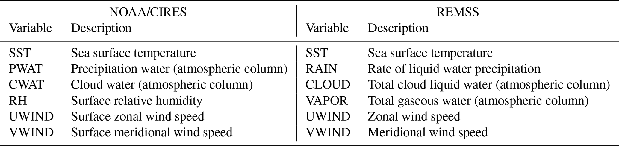
Note: The reanalysis dataset is provided by NOAA/CIRES, which is from January 1850 to December 2015 with 2 by 2^∘, and the remote sensing dataset is provided by REMSS, which is from December 1997 to August 2020 with 0.25 by 0.25^∘. In REMSS, UWIND and VWIND is collected from REMSS/CCMP (https://www.remss.com/measurements/ccmp/, last access: 15 November 2021), and other variables are collected from REMSS/TMI (1997–2012, http://www.remss.com/missions/tmi/, last access: 15 November 2021) and REMSS/AMSR2 (2012–2020, http://www.remss.com/missions/amsr/, last access: 15 November 2021). We try to choose physical variables in NOAA/CIRES with the same meaning as that in REMSS, such as CWAT, CLOUD, RH, and VAPOR. Limited by these two datasets, some variables can only find the closest match though they describe the different characteristics in ocean–atmosphere cycle, such as PWAT and RAIN.

To greatly increase the quantity of training data, we utilize the transfer learning technique to train our model with long-term climate reanalysis data and high-resolution remote sensing data progressively. These two datasets both provide multivariate global gridded data. The reanalysis data are supported by NOAA/CIRES (https://rda.ucar.edu/datasets/ds131.2/index.html, last access: 15 November 2021), which is a 6-hourly multivariate global climate dataset from January 1850 to December 2015 with 2^∘. The remote sensing data are obtained from Remote Sensing Systems (REMSS, http://www.remss.com/, last access: 15 November 2021), which is a daily multivariate global climate dataset from December 1997 to August 2020, and the resolution is much higher than reanalysis data with 0.25^∘. According to our chosen physical variables, we obtain the corresponding sub-datasets, and all the variables are preprocessed and averaged monthly. The detailed dataset descriptions are shown in Table 1. Note that we try to choose physical variables in NOAA/CIRES with the same meaning as that in REMSS, such as CWAT, CLOUD, RH and VAPOR. Some variables can only find the closest match in these two datasets though they describe the slightly different characteristics in ocean–atmosphere cycle, such as PWAT and RAIN.

In addition, we also collect the historical Niño 3, Niño 4, and Niño 3.4 index data from the China Meteorological Administration National Climate Centre (https://cmdp.ncc-cma.net/, last access: 15 November 2021). We pick up the records from January 2014 to August 2020 for the result analysis of following experiments.

The major active region of ENSO is concentrated in the tropical Pacific, so we crop the multivariate data with the region (40^∘ N–40^∘ S, 160^∘ E–90^∘ W) as the geographic boundaries of ENSO-ASC, which covers Niño 3 and Niño 4 regions. The reanalysis data have the size (40, 55) for every single-month variable, and the remote sensing data have the size (320, 440). In order to unify and improve dataset quality, we use bicubic interpolation (Keys, 1981) to enlarge the reanalysis data by 8× magnification and a soft-impute algorithm (Mazumder et al., 2010) to fill up missing values in both datasets. We train the model first on the whole reanalysis dataset and subsequently on the remote sensing dataset from December 1997 to December 2012 for fine-tuning. The samples from January 2014 to August 2020 in the remote sensing dataset are considered as the validation set. There is a 1-year gap between the fine-tuning set and validation set to reduce the possible influence of oceanic memory.

4.2 Experiment setting

We train and evaluate the ENSO-ASC on a high-performance server. Based on our proposed model, some hyper-parameter settings are determined by referring to the existing computing resources as following: K=4, $d_{\mathrm{1}}=d_{\mathrm{2}}=\mathrm{16}$, which is the optimal parameter combination after extensive experiments (this process has been ignored because it is not the focus in this paper). Adjacency matrix A and corresponding Laplacian matrix $\stackrel{\mathrm{̃}}{\mathbf{L}}$ are designed as in Sect. 3. All the following analyses are based on the stable results through repeated experiments.

We evaluate the ENSO-ASC from three aspects. Firstly, according to our proposed ENSO forecast formalization in Eqs. (5) to (7), there are several factors that may influence the performance from the perspective of model structure: the input sequence length M, the multivariate coupler coupler(•), the attention weights α and β, and the benefits of transfer training. We design some comparison experiments to investigate the model performance and determine the optimal model structure. A comparison with the other state-of-the-art models is also included. Secondly, we evaluate the forecast skill of the ENSO-ASC from the meteorological aspects according to Eqs. (5) to (7): the contributions of different input physical variables V in the pre-designed coupling graph G, the effective forecast lead month in IMS strategy, the forecast skill with different start calendar month scm, and the spatial uncertainties in longer-term forecasts. Finally, we forecast the real-world ENSO over the validation period and compare our results with the observations.

4.3 Evaluation of model performance

4.3.1 Influence of the input sequence length

Input sequence length M is very important for the forecasting model, due to the rich spatial–temporal information contained in it. In general, the longer sequence length M, the better the ENSO forecast skill. However, a longer input sequence will also increase the computational burden and raise the requirements for data quantity and quality in the training and calculation of complex deep learning networks, especially under such a high resolution of our model. Therefore, the balance between forecast performance and efficiency must be considered. We gradually increase the sequence length M to detect the changes in forecast skills. Figure 10 displays the results. As the sequence length gradually increases, two metrics become better (larger). When the sequence length is greater than 3 months, the growth rate slows down. While the sequence length is less than 3 months, the forecast skill increases rapidly.

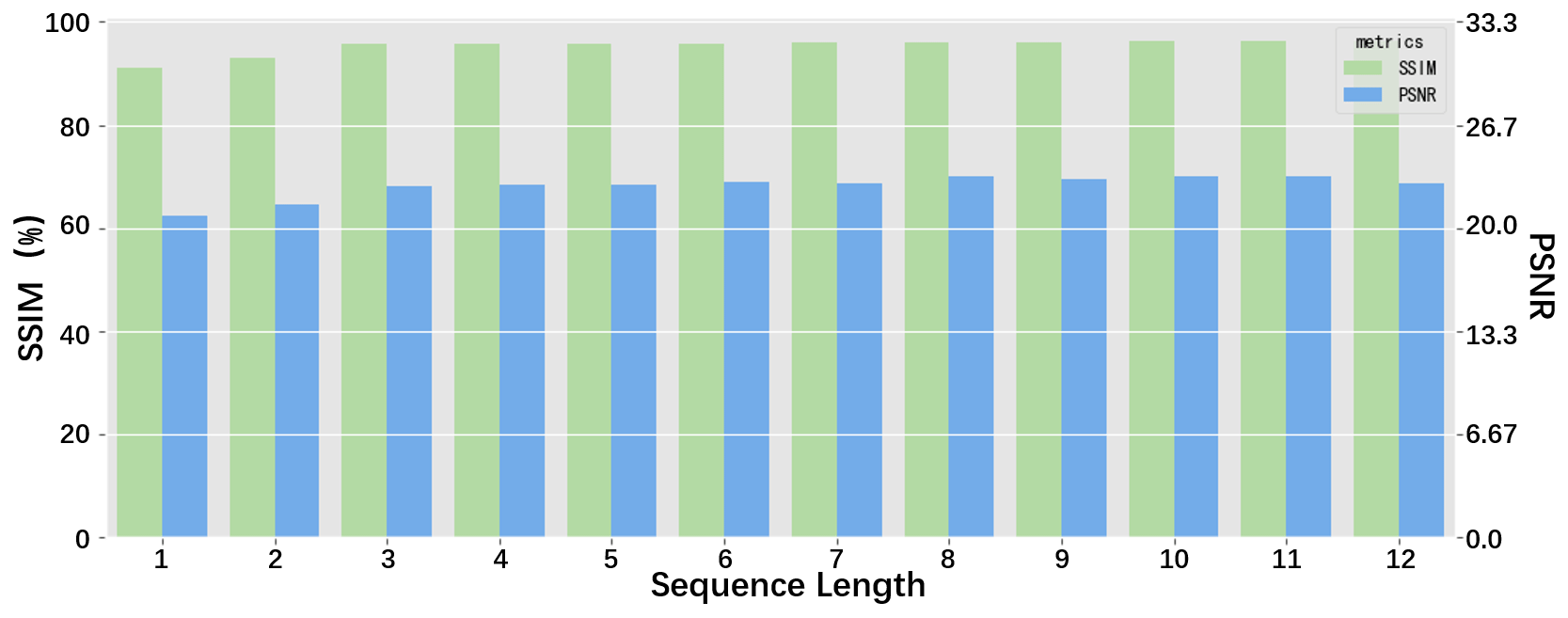
Figure 10 The performances of the ENSO-ASC when the input sequence length increases under IMS forecast strategy.

It is obvious that the increase in sequence length cannot lead to an unlimited improvement in forecast skill. In ENSO-ASC, making predictions with the previous 3 months' multivariate data is a more efficient choice. In fact, lots of successful works imply that a climate deep learning model does not require a longer input sequence to make skilful predictions, such as using previous 2 continuous time-step data to estimate the intensity of tropical cyclone (R. Zhang et al., 2019) and using previous 3-month ocean heat content and wind to predict ENSO evolution (Ham et al., 2019). A long-term temporal sequence contains strong trends and periodicities, but the underlying chaos is more dominant, which seriously hinders the prediction. The subsequent experiments will all apply the historical 3-month multivariate sequence (M=3) as model input.

4.3.2 Benefit of the transfer learning

For the model training, we use the transfer learning to overcome the insufficient sample challenge and obtain the optimally trained model. More specifically, we first train the model on a reanalysis dataset with 90 epochs and subsequently on a remote sensing dataset until total convergence (about 110 epochs). Here, 90 epochs are enough for training the ENSO-ASC on the reanalysis dataset until convergence, because the interpolated reanalysis data are smoother and lack details, which leads to easy training. In order to verify the benefit of the transfer learning, we also make comparative experiments by only training our model on a remote sensing dataset. The training process needs more epochs (such as 200 epochs), because the remote sensing dataset contains much more detailed high-level climate information.

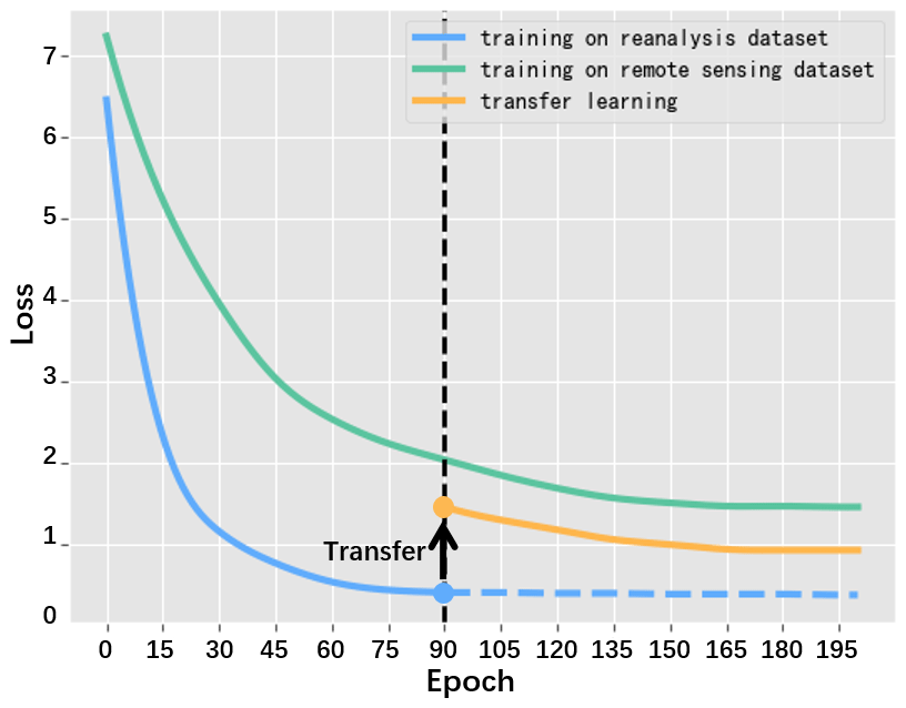
Figure 11 The loss changes when training with only reanalysis dataset (blue line), with only remote sensing dataset (green line) and transfer learning on these two datasets in order (black arrow and yellow line after 90 epochs).

The averaged loss changes for different training sets are depicted in Fig. 11. We can see that when training with the reanalysis dataset, the loss drops quickly, while when training with the remote sensing dataset, the model converges slowly and the loss is large. After using transfer learning, the loss on the remote sensing dataset are improved at least 15 %, which demonstrates that the systematic errors of ENSO-ASC are indeed corrected to some extent.

Comparing with remote sensing dataset, training with reanalysis dataset always yields a much smaller loss. It is due to the smoothness and lack of details of the reanalysis dataset as mentioned above that to the model can learn the characteristics more easily. However, the high-resolution remote sensing dataset reflects the real-world status more accurately, which contains more comprehensive and nonlinear details and amplitudes under a high resolution. If we have efficient remote sensing data, the forecast skill will be further improved.

4.3.3 Effectiveness of the multivariate air–sea coupler

We subjectively incorporate a priori ENSO coupled interactions into the graph-based multivariate coupler and select six critical physical variables as the predictors of the ENSO-ASC. The formalization not only treats each physical variable as a separate individual but emphasizes the nonlinear interactions between them. However, it is not clear whether such graph formalization is the reason for the improvement of ENSO forecast performance. In order to validate the effectiveness of our proposed formalization, we design two other deep learning couplers for ENSO forecast with the same datasets and transfer learning and then compare the performance with the ENSO-ASC.

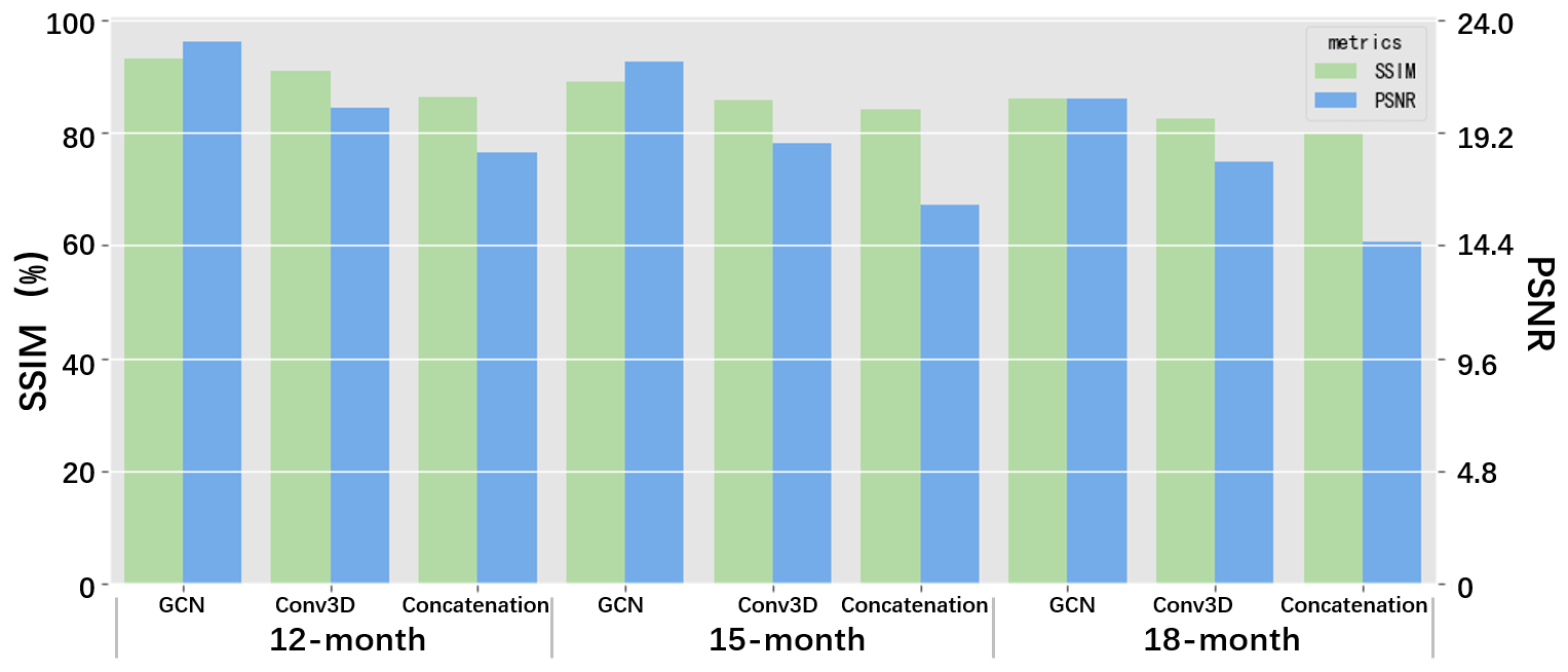
Figure 12 The performances of the ENSO-ASC when replacing the multivariate air–sea coupler with other deep learning structures.

The first coupler replaces GCN with a dual-layer 3D-convolution block, which treats all variables as a whole system and ignores the specific directions and neighbor-orders in coupling interactions between them. The second coupler just replaces the GCN with the concatenation of features from multivariate encoders, which treats the multiple variables as the channel stacking (or data overlay) and simply extracts global features of them together (the cascaded multivariate features are propagated to the decoders for every variable directly). The results are illustrated in Fig. 12. Obviously, our graph formalization achieves the best performance with measurements of SSIM and PSNR; the Conv3D coupler is slightly worse. The results indicate that using a graph to simulate multivariate interactions is a more reasonable approach, which can learn more ENSO-related dynamical interactions and underlying physical processes than other formalizations. Besides this, the comparative experiments also exhibit some inspiration: when building a climate forecast deep learning network that incorporates physical mechanisms, it is necessary to customize a suitable structure to represent and reflect specific mechanisms mathematically.

We design a fully connected adjacency matrix A in a GCN coupler, which means we consider that all physical variables have interactions with each other. Conv3D also entirely extracts the features of all variables. Under these circumstances, why does a GCN coupler have better performance than Conv3D coupler? From the perspective of mathematics, GCN will consider the pair-wise coupling between variables and learn the features of every coupled interaction according to the hidden nonlinearity in samples individually as in Eq. (12). But the Conv3D coupler inherits the characteristics of the global sharing and local connection in classic convolution, which rather treats all variables equally and lack descriptions of the special interactions.

4.3.4 Effects of attention weights

We customize two attention weights in the model to dynamically represent the effects of different temporal memories and multiple variables. Here, we analyze the influences of two proposed self-supervised attention weights by removing one of them from ENSO-ASC; the results are illustrated in Fig. 13. The results suggest the prediction skill will decline when one of the attention weights is removed. More specifically, the reduction of performance is larger when the multivariate attention is removed for shorter forecasts (less than about 9 months), and when the temporal attention is removed for longer forecasts (more than about 15 months). This is because of higher multivariate correlations and lower temporal non-stationarity in the short term. But the temporal memory effects dominate the long-term evolution.

Figure 13 The performances of the ENSO-ASC when removing one of the attention weights.

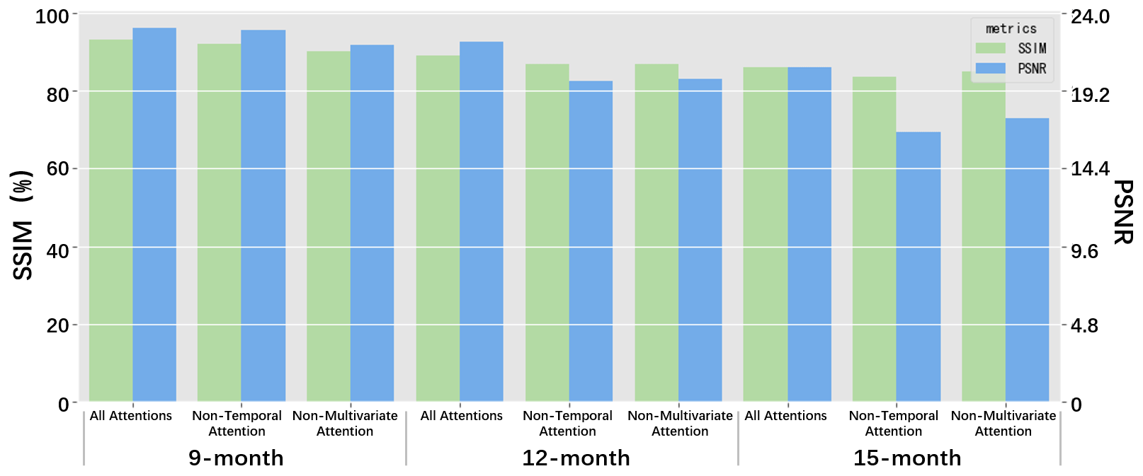
In fact, due to the self-supervised attentive weights α and β, though the multivariate graph and model structure are fixed, the forecast skills will not change too much with the different start calendar months and variable combinations (see Sect. 4.4). However, if these two weights are unset, the model will not be able to distinguish the contributions of multivariate oceanic memories in different forecast start months adaptively, seriously misleading the forecasts.

Indeed, it may be a better choice for ENSO forecast to establish and filter the optimal model for different start calendar months, forecast lead times, and various predictors, but it also consumes more resources and time. These two attentive weights α and β can reasonably prune the model within the acceptable range of prediction errors. In operational forecasts, separate modeling for different scenarios can be used to pursue higher accuracy and skills.

4.3.5 Comparison with other state-of-the-art ENSO deep learning models

We compare the ENSO-ASC with other state-of-the-art data-driven ENSO forecast models, including (1) convolutional neural networks (encoder–decoder structure with 12 layers, which has the same trainable layer number with our model); (2) long short-term memory networks (6 LSTM layers and final fully connect layer); (3) a ConvLSTM network (CL-6 means a 6-layer structure, CL-12 means a 12-layer structure); and (4) a 3D-convolution coupler to simulate multivariate interactions as mentioned above (Conv3D). In order to ensure the fairness of the comparison, we utilize the same input physical variables, training and validation datasets, and training criteria for the above models, then train them via transfer learning with plenty of epochs to achieve their optimal performances. Table 2 displays the comparative results with 12-, 15-, and 18-month forecasts. In general, the forecast models considering ENSO spatial–temporal correlations (e.g., ConvLSTM, Conv3D) outperform the basic deep learning models (e.g., CNN, LSTM), which implies that the complicated network structures can mine the sophisticated dependencies deeply hidden in long-term ENSO evolutions more effectively. As the lead time increases, the performances of models gradually decrease. However, the ENSO-ASC still maintains high accuracy and is always better than other models with an improvement of about 5 %, which indicates the superiority of our model.

Table 2 Performance comparisons with other state-of-the-art deep learning models.

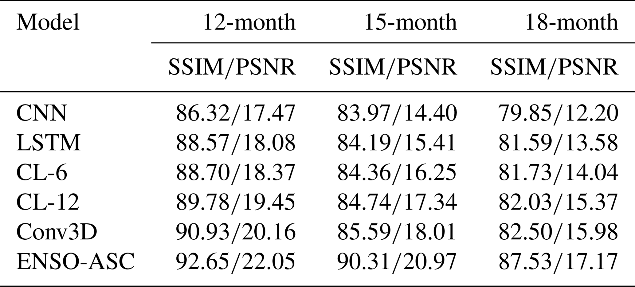
Considering the calculation ingredients of PSNR and SSIM according to Eq. (11): the calculation of PSNR contains MSE, which is the metric for individual grids, while SSIM measures the spatial characteristics and distributions of two patterns from many correlation coefficients, which can represent a measurement for evolution tendency and physical consistency to some extent. Based on the above analysis, Table 2 also indicates that the forecast results of ENSO-ASC exhibit an excellent physical consistency beyond other models, the SSIM of which is much better, especially in the longer lead time. In addition, the ENSO-ASC pays more attention to the detailed spatial distributions, which is beneficial for the further analysis of ENSO dynamical mechanisms.

On the other hand, the ENSO-ASC is the first attempt to forecast ENSO at such a high resolution (0.25^∘). Despite the difficulty of training increasing, our model still achieves good results. Interestingly, though the ENSO-ASC involves the most trainable parameters, its convergence epoch is one-fifth on average of other forecast models.

4.4 Analysis of ENSO forecast skill

4.4.1 Contributions of different predictors to the forecast skill

The superiority of our proposed model derives from the graph formalization, and the special multivariate coupler can effectively express the processes of synergies between multi-physical variables. From another perspective, the improvement of the forecast skill is not only due to graph formalization, but also the utilization of multiple variables highly related to ENSO compared to using limited variables to predict ENSO as in previous works. For ENSO forecasting, SST is definitely the most critical predictor. Besides SST, other variables have different contributions to the forecast results. Therefore, we design an ablation experiment by removing one of predictors from our proposed model and detect the reduction of forecast skill (Table 3 above). Meanwhile, we also add one extra predictor (from surface air temperature, surface pressure, and ocean heat content respectively) into our proposed model to investigate the improvement of forecast skill (Table 3 below). Here, the input sequence length is still set to 3.

Table 3 Model performance when one existing variable is removed or one extra variable is added.

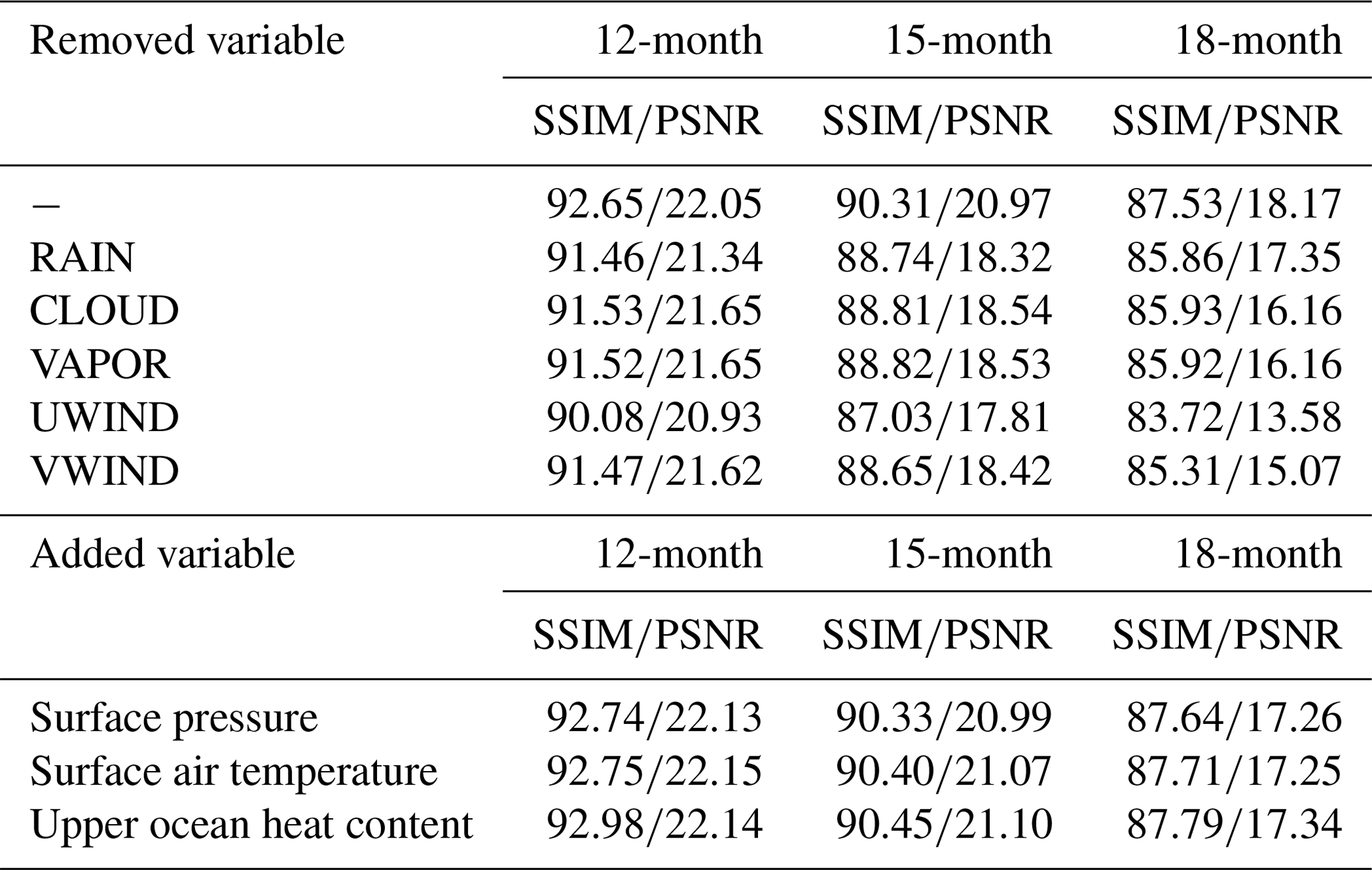
Table 3 (above) shows that when a variable is removed from the input of the deep learning model, the ENSO forecast skill will be reduced. More specifically, when the zonal wind speed (UWIND) is removed, the reduction is the largest. From the perspective of ENSO physical mechanism, zonal wind anomalies (ZWAs) always play a necessary role and are even considered as the co-trigger or driver of ENSO events. As an atmospheric variable, ZWA often gives a direct feedback on oceanic varieties with a shorter response time than oceanic memory. ENSO-ASC uses historical 3-month multivariate data to predict ENSO evolution, which is quite a short sequence length. Under such sequence length, wind speed (including u wind and v wind) has a relatively high correlation with SST. In addition, RAIN is another variable that slightly affects the forecast. This is because the precipitation process has a straightforward contact with the sea surface, and the energy transfer is easier.

Table 3 indicates that the model performance improves a little when adding surface air temperature, surface pressure, and ocean heat content into the multivariate coupler. This is because the multivariate graph with existing variables in the ENSO-ASC can almost describe a relatively complete energy loop in the Walker circulation, so the effects of the extra added variables to the ENSO forecasts are not obvious. It is worth noting that the input sequence length should be longer when feeding the ocean heat content into the multivariate coupler, because this predictor has long memory (Ham et al., 2019; McPhaden, 2003; Jin, 1997; Meinen and McPhaden, 2000). However, as the input sequence length varies from 3 to 9 months, the forecast skills of ENSO-ASC have not actually changed much. This is mainly because the global spatial teleconnections and temporal lagged correlations by the Walker circulation and ocean waves (such as Kelvin and Rossby waves) (Exarchou et al., 2021; Dommenget et al., 2006) are not caught in the model, the input region of which mainly covers the equatorial Pacific. In addition, the model contains only one long memory predictor besides SST.

Among the three extra added physical variables, the upper ocean heat content is a very concerning variable, which can reflect the vertical and horizontal propagations of ocean waves and help interpret the dynamical mechanisms. Therefore, we conduct the comparison via two modified ENSO-ASC models with the same output of SST + u wind, v wind, rain, cloud, and vapor, while with the different input. One uses upper ocean heat content + u wind, v wind, rain, cloud, and vapor, marked as EXAM; another uses SST + u wind, v wind, rain, cloud, and vapor, marked as CTRL. The results are shown in Table 4.

Table 4 Model performance comparison when using upper ocean heat content to replace SST in the input.

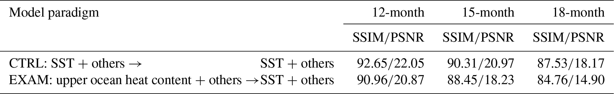
Note: Model paradigm represents the input and the output for the ENSO-ASC, where → means “forecast”. “Others” represents five variables, including u wind, v wind, rain, cloud, and vapor. The first row is the control experiment, which is the same with the result in Table 3, and the second row is the examined experiment, which replaces SST by the upper ocean heat content in the model input.

The forecast skill of EXAM is slightly lower than CTRL. The upper ocean heat content is the average of the oceanic temperature from the sea surface to the upper 300 m. When using it as a predictor to forecast SST, our model will extract the features of oceanic temperature not only from sea surface but also from the deeper ocean, which inevitably introduces more noise. This may be a reason for the above result. Therefore, we still use SST instead of the upper ocean heat content as the key predictor which would bring higher forecast skills.

In the subsequent experiments, the model will use the chosen 6 variables (SST, u wind, v wind, rain, cloud, and vapor), and the input sequence length is set to 3.

4.4.2 Analysis of effective forecast lead month

The accuracy of long-term prediction is the most crucial issue for meteorological research. In ENSO events, though the periodicity dominates the amplitude, the intrinsic intensity and duration often induce large uncertainties and forecast errors. Therefore, over the validation period, we make predictions with multiple lead times and calculate the corresponding Niño indexes from the forecasted SST patterns to investigate the effective forecast lead month of our model. The correlations between forecasted Niño indexes and the official records are depicted in Fig. 14. As the lead time gradually increases to 24 months, the correlation skill slowly decreases. It is worth noting that when the lead time is from 10 to 13 months, the reduction of the forecast skills slows down a little. This is because the periodicity in ENSO events becomes stronger after a 1-year iteration in IMS strategy. These results demonstrate that the ENSO-ASC can provide reliable predictions up to at least 18 to 20 months on average (with correlations over 0.5). Within a 6-month lead time, the correlation skill is over about 0.78, and from a 6- to 12-month lead time, correlation skill is over about 0.65.

Figure 14 The correlation skills between the forecast results of the ENSO-ASC and real-world observations on three Niño indexes with the forecast lead time increasing over the validation period.

In addition, the forecast skills for the Niño 3 index and Niño 3.4 index are a little higher than that of Niño 4 index. This indicates that our model has higher forecast skill for the EP-El Niño events (the active area of SST anomalies is mainly over the eastern tropical Pacific Ocean) than the CP-El Niño events (the active area of SST anomalies is mainly over the western and central tropical Pacific Ocean). This is because the input area of the model mainly covers the entire tropical Pacific, which can be considered as the sensitive area for EP-El Niño events and is more favorable for the prediction of EP-El Niño events. As for the prediction of CP-El Niño events, extratropical Pacific or other oceanic regions may have stronger impacts on the western–central equatorial Pacific (Park et al., 2018).

4.4.3 Temporal persistence barrier with different start calendar months

Deep learning models can extend the effective lead time of ENSO forecasts, which means it can raise the upper limitation of ENSO prediction to some extent. From the perspective of IMS strategy, if a well-trained model can predict next-month SST perfectly (in other words, with a very low prediction error), the model can iterate a lot theoretically. However, our proposed model is affected by a variety of factors, which leads to performance degradation.

One of the disadvantages in IMS strategy is that once a relatively large forecast error shows up in a certain iteration, such a forecast error will be continuously amplified in subsequent iterations. In ENSO forecasting, such a forecast skill decline is regarded as a persistence barrier and usually occurs in spring (i.e., spring predictability barrier, SPB) (Webster, 1995; Zheng and Zhu, 2010). SPB limits the long-term forecast skill in not only numerical models but some other statistical models (Kirtman et al., 2001). For further investigation into the performance degradation, we firstly make continuous predictions over the validation period from different start calendar months with different lead times and then calculate the correlations between the calculated Niño 3.4 index with the official records. Figure 15 shows the results.

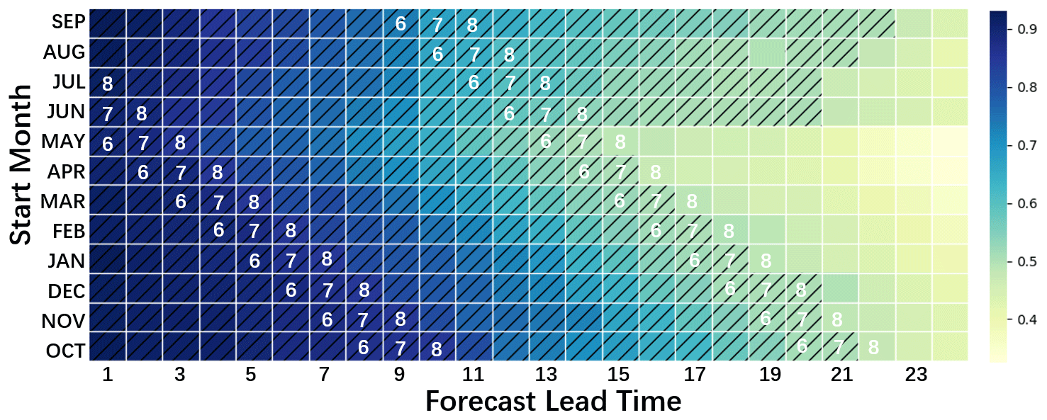
Figure 15 The correlation skill heat map between the forecast results of the ENSO-ASC and real-world observations on Niño 3.4 index with different forecast start months over the validation period. The hatching cells represent the correlations exceed 0.5, and the white numbers on the cells mean the calendar months.

In Fig. 15, the darker the cells' color, the higher the correlations between the forecast and observation, the higher the forecast skill. The hatching cells represent that the correlations exceed 0.5. Overall, making ENSO forecast with start calendar months MAM (March, April, and May) is not very reliable, while the long-term forecast of ENSO is more accurate with start months JAS (July, August, and September). In addition, there exist two obvious color change zones among all cells, which means the correlations drop significantly in such zones (cell color becomes lighter), and both of them occur in the months JJA (June, July, and August) depicted as the white numbers on the cells. The first zone reduces the correlations by about 0.03, and the second zone makes the reduction by about 0.06. It demonstrates that when making forecasts through the months JJA, the ENSO predictions tend to be much less successful. This is why the model exhibits more skilful forecasts with the start months JAS, which avoids forecasting through the months JJA as much as possible and preserves more accurate features during iterations, resulting in a relatively long and efficient lead time. Analogous to SPB in traditional ENSO forecasting, our proposed ENSO-ASC has a forecast persistence barrier in boreal summer (JJA). This may be because the real-world dataset contains more frequency CP-El Niño samples after 1990s (Kao and Yu, 2009; Kug et al., 2009), which are significantly impacted by the summer predictability barrier (Ren et al., 2019; Ren et al., 2016). At the same time, it also implies that there are still forecast obstacles that need to be circumvented in the ENSO deep learning forecast model, and more unknown key factors need to be considered and explored, such as more variables, larger input regions, more complex mechanisms, etc. Great progress will be made by building deep learning models based on prior meteorological knowledge in the future.

4.4.4 Spatial uncertainties with a longer lead time

In ENSO forecasts, the areas where the forecast uncertainties occur are usually not randomly distributed, and such areas should be given more attention in operational target observation. Over the validation period, we make 12-month and 18-month forecasts and then compare the forecast results with observations. More specifically, we calculate covariance between forecast sequence $\widehat{s}$ and observation s for every grid point and combine them as a spatial heat map.

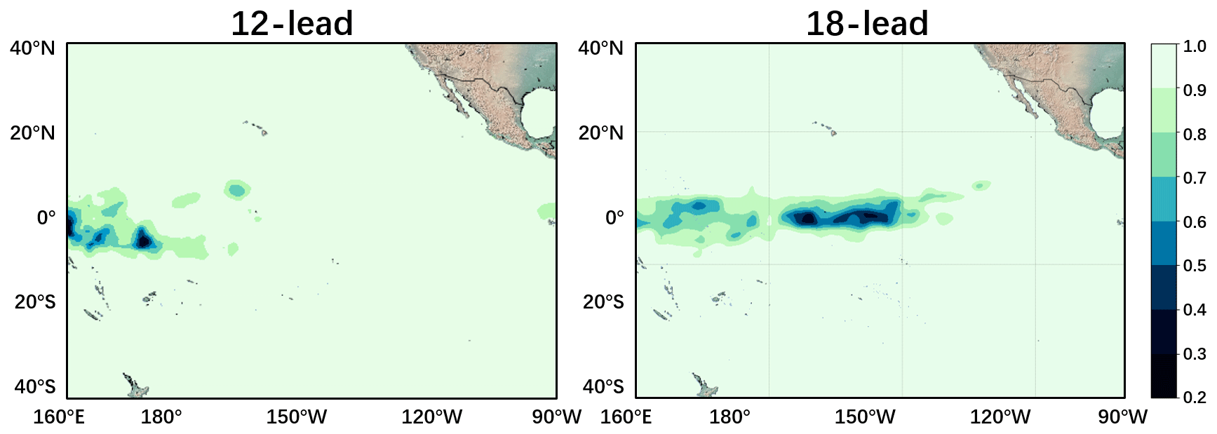
Figure 16 The spatial covariance heat map between the forecast results of the ENSO-ASC and real-world observations with 12 and 18 lead months over the validation period.

The results are shown in Fig. 16. The spatial uncertainties first show up over the western equatorial Pacific, and then as the lead time increases, the uncertainty area gradually expands eastward to the central equatorial Pacific. It indicates that the Niño 3 and Niño 3.4 regions both have very high forecasting skills with a short forecast lead time (See Fig. 14 in 12-month forecast), while the predictability for the central equatorial Pacific gradually drops with a longer lead time, which leads to a rapid reduction of forecast skill for Niño 3.4 and Niño 4 regions shown as a 15-month forecast in Fig. 14. This reminds us that the areas with larger forecast uncertainties should be observed using a higher frequency. Besides this, another possible reason is that the multivariate input region is confined to the Pacific, but the ocean–atmosphere coupling interactions in the western tropical Pacific can be profoundly influenced by extratropical Pacific areas and other ocean basins as mentioned above. Therefore, our proposed model has relatively weak ability to capture the development of SST over the western–central equatorial Pacific.

4.5 Simulation of the real-world ENSO events

Since the 21st century, the occurrences of ENSO are more and more frequent. In particular, the duration and intensity of ENSO have largely changed. For example, many numerical climate models failed to forecast the 2015–2016 super El Niño. We simulate several ENSO events during the validation period and compare the forecast results with real-world observations. As mentioned above, wind (u wind and v wind) is also a relatively important and sensitive predictor in the ENSO-ASC for ENSO forecasts. Therefore, we make long-term forecasts and mainly trace the evolutions of SST and wind (u wind and v wind). Note that all of the following patterns describe the evolutions of SST and wind anomalies by subtracting the climatology (climate mean state, the monthly averaged SST and wind from 1981 to 2010) of that month from the forecasted SST and wind patterns.

Figure 17 The growth phase of SST and wind anomalies in the 2015–2016 super Niño event from April 2015 to June 2015. Panels (a)–(c) show the forecast results of the ENSO-ASC and (d)–(f) show real-world observations.

Figure 17 displays the evolutions of SST and wind anomalies in the growth phase of the 2015–2016 super El Niño event from April to June 2015, where (a)–(c) sub-figures are forecasts and (d)–(f) sub-figures are observations. Figure 18 displays the peak phase from September 2015 to February 2016, where (a)–(f) sub-figures are forecasts and (g)–(l) sub-figures are observations. These two results are both with the forecast start time of January 2015. During the growth phase, the warming SST anomalies first show up over the eastern tropical Pacific Ocean, which reduce the east–west gradient of SST. Meanwhile, the westerly wind anomalies over the western–central equatorial Pacific further enhance the SST anomalies over the central–eastern equatorial Pacific and weaken the Walker circulation (Fig. 17a–c). The SST and wind anomalies trigger the Bjerknes positive feedback together, which causes SST anomalies to be continuously amplified. During the peak phase, in addition to the local evolutions of the equatorial Pacific SST anomalies, there are obvious warm SST anomalies over the northeast subtropical Pacific near Baja, California, induced by the extratropical atmospheric varieties (Yu et al., 2010; Yu and Kim, 2011), which gradually propagate southwestward and merge with the warm SST anomalies over the central equatorial Pacific (Fig. 18a–d). In conclusion, the ENSO-ASC can track the large-scale oceanic–atmospheric varieties steadily and can successfully predict the ENSO with strong intensity and long duration, while many dynamic or statistical models fail. At the same time, our proposed model makes the prediction at the beginning of the calendar year and produces a quite low prediction error, which demonstrates that the model can overcome or eliminate the negative impacts of SPB to some extent.

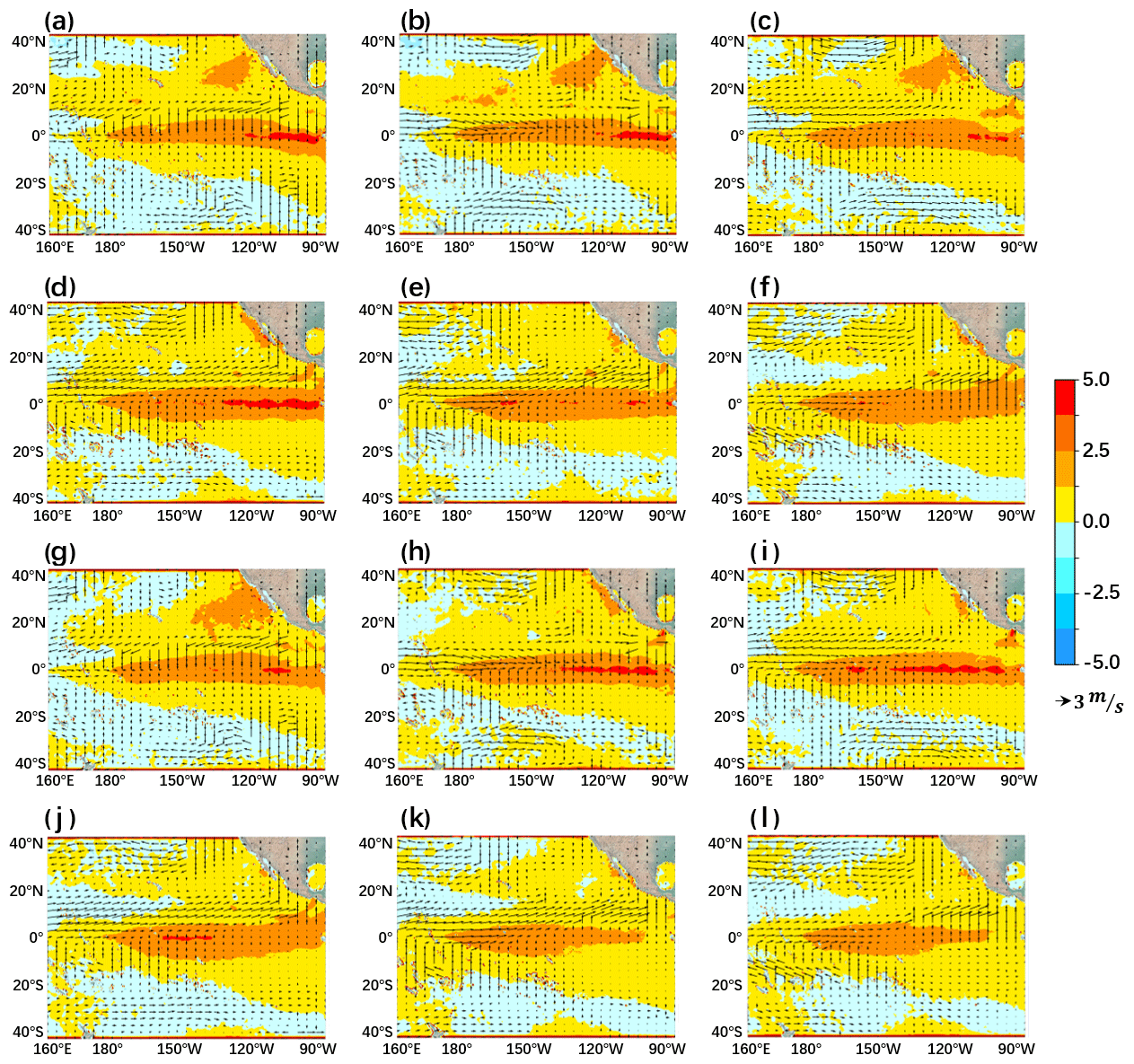
Figure 18 The peak phase of SST and wind anomalies in the 2015–2016 super Niño event from September 2015 to February 2016. Panels (a)–(f) show the forecast results of the ENSO-ASC and (g)–(l) show real-world observations.

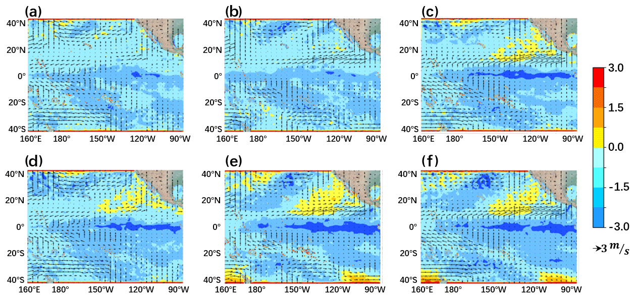
Figure 19 The same with Fig. 17 but for the growth phase of SST and wind anomalies of 2017 weak La Niña event from September to November 2017.

Besides the super El Niño event, the ENSO-ASC also has high simulation capabilities for weak nonlinear unstable evolutions. In reality, neutral or weak events actually account for most of the time. Judging from the saliency of the extracted features, neutral or weak events may contain more “mediocre and fuzzy” characteristics, which lead to some difficulties in accurately grasping their meta features during evolutions. For example, it is much easier to overestimate or underestimate their intensities. Therefore, we chose a hindcast over the validation period. Figure 19 shows the peak phase of a weak La Niña event from September to November 2017 with the forecast start time of June 2016, where (a)–(c) sub-figures are forecasts and (d)–(f) sub-figures are observations. From its evolution, there are negative SST anomalies over the eastern equatorial Pacific and easterly wind anomalies in the western tropical Pacific Ocean, which will enhance the Walker circulation. In addition, Bjerknes positive feedback is the dominant factor favoring the rapid anomaly growth in this simulation.

Figure 20 The same with Fig. 17 but for the neural SST and wind anomalies evolutions in January to March 2020.

Another ENSO forecast limitation is to predict the neural year as the event of El Niño (or La Niña), which is also known as the false alarm rate. Figure 20 displays the neutral event from January to March 2020 with the forecast start time of January 2019 (its ONI has not yet reached the intensity of El Niño). After calculating the corresponding Niño index, we can determine that the ENSO-ASC can accurately avoid the false alarm and credibly reflect the real magnitude of the development of important variables such as SST. We have also verified the case in 2014 and the result is consistent with the facts. Many operational centers erroneously predicted that an El Niño would develop in 2014, but it did not.

The forecasted SST and wind anomaly patterns have a consistent intensity and tendency with the observations. Our model can achieve better forecast skills in a variety of situations because our proposed deep learning coupler comprehensively absorbs the sophisticated oceanic and atmospheric varieties, and its deep and intricate structure can almost simulate the air–sea energy exchange simultaneously, while traditional geoscience fluid programming in numerical climate models usually applies interval flux exchange and parameterized approximation for unknown mechanisms, blocking the continuous interactions.

5 Discussions and conclusions

ENSO is a very complicated air–sea coupled phenomenon, the life cycle of which is closely related to the large-scale nonlinear interactions between various oceanic and atmospheric processes. ENSO is one of the most critical factors that cause extreme climatic and socioeconomic effects. Therefore, meteorological researchers are starting to find more accurate and less consuming data-driven models to forecast ENSO, especially deep learning methods. There are already many successful attempts that have extended the effective forecast lead time of ENSO up to 1.5 years. They all extract the rich spatial–temporal information deeply hidden in the historical geoscience data.

However, most of the models use limited variables or even a single variable to predict ENSO, ignoring the coupling multivariate interactions in ENSO events. At the same time, the generic ENSO deep learning forecast models seem to have reached the performance bottleneck, which means deeper or more complex model structures can neither extend the effective forecast lead time nor provide a more detailed description for dynamical evolutions. In order to overcome these two barriers, we subjectively incorporate a priori ENSO knowledge into the deep learning formalization and derive hand-crafted features into models to make predictions. More specifically, considering the multivariate coupling in the Walker circulation related to ENSO amplitudes, we select six indispensable physical variables and focus on the synergies between them in ENSO events. Instead of simple variable stacking, we treat them as separate individuals and ingeniously formulate the nonlinear interactions between them on a graph. Based on such formalization, we design a multivariate air–sea coupler (ASC) by graph convolution mathematically, which can mine the coupling interactions between every physical variable in pairs and perform the multivariate synergies simultaneously.

We then implement an ENSO deep learning forecast model (ENSO-ASC) with the encoder–coupler–decoder structure, and two self-supervised attention weights are also designed. The multivariate time-series data are firstly propagated to the encoder to extract spatial–temporal features respectively. Then the multivariate features are aggregated together for interactions in the multivariate air–sea coupler. Finally, the coupled features are divided separately, and the corresponding feature of a certain variable is restored to forecast patterns in the decoder. IMS strategy is applied to make predictions, which is a more stable forecasting method. We use transfer learning to provide a better model initialization and overcome the problem of a lack of observation samples. The model is first trained on the reanalysis dataset and subsequently on the remote sensing dataset. After constructing the model structure, we design extensive experiments to investigate the model performance and ENSO forecast skill. Several successful simulations in the validation period are also provided. Some conclusions can be summarized as follows:

1. According to the forecast model described in Eqs. (5) to (7), we adjust the model settings of the input sequence length M, the multivariate coupler coupler(•), the attention weights α and β, and the transfer training and then investigate the performance changes. The optimal input sequence length of the model is 3 according to the trade-off between forecast skill and computational resource consumption. It implies that the ENSO deep learning forecast model does not need a relatively long-sequence input. Although the long sequence contains a rich tendency and periodicity of ENSO events, the meteorological chaos is more dominant, which seriously hinders the prediction. Transfer learning is a practical method. Training the model on the reanalysis dataset and subsequently on the remote sensing dataset can effectively reduce the systematic forecast errors by at least 15 %. When replacing the graph-based multivariate air–sea coupler in ENSO forecast model with other deep learning structures, the forecast skill drops obviously. This demonstrates that the graph formalization is a powerful expression for simulating underlying air–sea interactions, and a corresponding the ENSO forecast model with novel multivariate air–sea coupler can forecast more realistic meteorological details. This also demonstrates that it is critical to choose suitable deep learning structures to incorporate prior climate mechanisms for improving forecast skills. The self-supervised attention weights are also promising tools to grasp the contributions of different predictors and memory varieties of different forecast start calendar months. In addition, in comparison with other state-of-the-art ENSO forecast models, the ENSO-ASC achieves at least 5 % improvement in SSIM and PSNR for long-term forecasts.

2. By performing the ablation experiment, the forecast skill drops significantly when removing the zonal wind from the model input, which is because it is a co-trigger of Bjerknes positive feedback in ENSO events and gives a direct feedback on oceanic varieties with a shorter lag time. Adding extra predictors can slightly improve the performance; this is because the existing multivariate graph can almost describe a relatively complete energy loop in the Walker circulation. By tracing the upper limitation of forecast lead time, the ENSO-ASC can provide a reliable high-resolution ENSO forecast up to at least 18 to 20 months on average judging from the correlation skills of Niño indexes greater than 0.5. Within a 6-month lead time, the correlation skill is over about 0.78, and from a 6- to 12-month lead time, correlation skill is over about 0.65. The corresponding correlation skills decline slowly from a 10- to 13-month lead time and then declined rapidly. This is because of the stronger periodicity in ENSO events after a 1-year iteration of IMS strategy. At the same time, the different forecast start calendar months also influence the forecast skills. The temporal heat map analysis shows that an obvious skill reduction usually shows up in JJA and produces a boreal summer persistence barrier in our model. In addition, from the spatial uncertainty heat map, our model exhibits larger forecast uncertainties over the western–central equatorial Pacific. Such spatial–temporal predictability barriers are widely present in dynamic or statistical models, but the ENSO-ASC effectively prolongs the forecast lead time and reduces corresponding uncertainties to a large extent.

3. Some successful simulations exhibit the effectiveness and superiority of the ENSO-ASC. We make real-world ENSO simulations during the validation period by tracing the evolutions of SST and wind anomalies (u wind and v wind). In the forecasted El Niño (La Niña) events, the sea–air patterns clearly display that the positive (negative) SST anomalies first show up over the eastern equatorial Pacific with westerly (easterly) wind anomalies in the western–central tropical Pacific Ocean, which induces the Bjerknes positive feedback mechanism. As for the 2015–2016 super El Niño, the ENSO-ASC captures the strong evolutions of SST anomalies over the northeast subtropical Pacific in the peak phase and successfully predicts its very high intensity and very long duration, while many dynamic or statistical models fail. ENSO-ASC can also credibly reflect the real situation and reduce the false alarm rate of ENSO such as that in 2014. In conclusion, our model can track the large-scale oceanic and atmospheric varieties and simulate the air–sea energy exchange simultaneously. It demonstrates that the multivariate air–sea coupler effectively simulates the oscillations of the Walker circulation and reveals more complex dynamic mechanisms such as Bjerknes positive feedback.

The extensive experiments demonstrate that the ENSO forecast model with a multivariate air–sea coupler (ENSO-ASC) is a powerful tool for analysis of ENSO-related complex mechanisms. Meteorological research does not only pursue skilful models and accurate forecasts but also requires a comprehensive understanding of the potential dynamical mechanisms. In the future, we will extend our model to more global physical variables with informative vertical layers, such as the thermocline depth, and the ocean temperature heat content, to explore the global spatial remote teleconnections, temporal lagged correlations, and the optimal precursor etc.