the Creative Commons Attribution 4.0 License.
the Creative Commons Attribution 4.0 License.
 | 11 Nov 2021
Ice Algae Model Intercomparison Project phase 2 (IAMIP2)
Hakase Hayashida
Meibing Jin
Nadja S. Steiner
Neil C. Swart
Eiji Watanabe
Russell Fiedler
Andrew McC. Hogg
Andrew E. Kiss
Richard J. Matear
Peter G. Strutton
Ice algae play a fundamental role in shaping sea-ice-associated ecosystems and biogeochemistry. This role can be investigated by field observations; however the influence of ice algae at the regional and global scales remains unclear due to limited spatial and temporal coverage of observations and because ice algae are typically not included in current Earth system models. To address this knowledge gap, we introduce a new model intercomparison project (MIP), referred to here as the Ice Algae Model Intercomparison Project phase 2 (IAMIP2). IAMIP2 is built upon the experience from its previous phase and expands its scope to global coverage (both Arctic and Antarctic) and centennial timescales (spanning the mid-20th century to the end of the 21st century). Participating models are three-dimensional regional and global coupled sea-ice–ocean models that incorporate sea-ice ecosystem components. These models are driven by the same initial conditions and atmospheric forcing datasets by incorporating and expanding the protocols of the Ocean Model Intercomparison Project, an endorsed MIP of the Coupled Model Intercomparison Project phase 6 (CMIP6). Doing so provides more robust estimates of model bias and uncertainty and consequently advances the science of polar marine ecosystems and biogeochemistry. A diagnostic protocol is designed to enhance the reusability of the model data products of IAMIP2. Lastly, the limitations and strengths of IAMIP2 are discussed in the context of prospective research outcomes.
- Article
(4331 KB) - Full-text XML
- BibTeX
- EndNote


Together with pelagic phytoplankton, microalgae that colonize sea ice are the foundation of polar marine food webs. Understanding the susceptibility of ice algae to climate change is therefore essential to comprehending the climatic impacts on higher trophic levels, such as fish, seals, whales, penguins, polar bears, and humans (Cavan et al., 2019; Darnis et al., 2012). Vernal blooms of ice algae also directly influence lower trophic levels, such as phytoplankton, zooplankton, and krill, by drawing down near-surface nutrients, reducing light transmission through sea ice, seeding subsequent pelagic blooms, and providing a food source for pelagic and benthic grazers (Leu et al., 2015). Ice algae also regulate ocean biogeochemistry through the biological carbon pump (Mortenson et al., 2020; Watanabe et al., 2015) and polar climates via the production of the climate-active trace gas dimethyl sulfide (Levasseur, 2013) and via the modification of sea-ice albedo (Zeebe et al., 1996).
Field observations of ice algae abundance and distribution are scarce, mainly due to logistical and methodological challenges in these remote and cold environments (Miller et al., 2015), even though technological advancements in recent years have enabled field sampling at much larger scales (Castellani et al., 2020; Cimoli et al., 2020; Lange et al., 2017). Satellite observations are incapable of detecting algae in sea ice. Therefore, the role of ice algae in polar marine ecosystems and biogeochemistry at the regional and global scales remains unclear. One approach to address this knowledge gap is numerical modelling, which simulates ice algae abundance and distribution across the sea-ice domain by incorporating a numerical model of the sea-ice ecosystem into a regional or global three-dimensional coupled sea-ice–ocean general circulation model (Vancoppenolle and Tedesco, 2017).
An initial model intercomparison effort was made recently to understand the similarities and differences in simulated ice algae abundance and distribution among the existing three-dimensional models (IAMIP1 hereafter; Watanabe et al., 2019). This model intercomparison investigated the seasonal-to-decadal variability in ice-algal primary productivity in four regions across the Arctic during 1980–2009 simulated by five participating models. The conclusions were (1) the decadal trend is unclear despite the ongoing reduction in Arctic sea ice; (2) the vernal bloom shifts to an earlier onset and briefer duration over the period of the simulations; and (3) the choice of the maximum growth rate is a key source of the inter-model spread in the simulated ice-algal primary productivity.
Polar regions, especially the Arctic, are warming faster than the rest of the globe, which results in the reduction in both Arctic and Antarctic sea ice (Smith et al., 2019). However, as demonstrated by the previous model intercomparison study (Watanabe et al., 2019), the transient response of ice algae to the anticipated loss of sea ice throughout the 21st century may not necessarily be linear. Using a one-dimensional sea-ice biogeochemistry model, Tedesco et al. (2019) found such a non-linear projected response of ice-algal primary productivity to global warming that also has strong latitudinal dependence. Further investigation using three-dimensional models will provide a comprehensive view of the climate change impacts on polar marine ecosystems and biogeochemistry at the regional to global scale, and determine whether ice algae exert any influence on global climate. This knowledge will help to clarify whether ice algae should be incorporated into the next generation of Earth system models (ESMs), such as those participating in the Coupled Model Intercomparison Project phase 6 (CMIP6; Eyring et al., 2016).
This paper introduces a new model intercomparison effort for ice algae, referred to here as the Ice Algae Model Intercomparison Project phase 2 (IAMIP2). IAMIP2 improves on the previous effort (IAMIP1) in its experimental design, which is based on the experimental protocols of CMIP6. A consistent experimental design allows us to provide more robust estimates of model bias and uncertainty and consequently advance the science of polar marine ecosystems and biogeochemistry. The scope of IAMIP2 is global, covering both the Arctic and Antarctic, and centennial timescales, spanning the mid-20th century to the end of the 21st century. IAMIP2 has five main objectives: (1) the evaluation of systematic bias in the existing sea-ice ecosystem models; (2) a mechanistic understanding of the past changes in ice algae abundance and distribution; (3) an assessment of projected changes and their uncertainty in ice algae abundance and distribution; (4) regional to global impacts on marine ecosystems and biogeochemistry; and (5) open-access distribution of the model output for sea-ice research and education.
To date, six three-dimensional coupled sea-ice–ocean models have been committed to participating in IAMIP2 (Table 1). These models represent either a global or regional configuration of the sea-ice and ocean components of the ESMs or global coupled models (GCMs) participating in CMIP6. A key difference from these parent model components is that the IAMIP2 models include sea-ice ecosystem components that simulate the biological sources and sinks of ice algae biomass and nutrient concentrations in the bottom-ice layer (Fig. 1). In each model, the sea-ice ecosystem component is coupled to the sea-ice component to account for physical processes that regulate the budgets of ice algae biomass and nutrient concentrations, such as sea-ice growth and melt. The sea-ice ecosystem component is also coupled to ocean dynamics and ecosystem components to simulate the tracer exchange at the sea-ice–ocean interface. Three of the IAMIP2 models are global configurations, while the other three are pan-Arctic regional configurations in which the tracer states in the ocean are prescribed at the lateral boundaries. The IAMIP2 models are driven by applying a common atmospheric forcing dataset at the surface boundary. We welcome the participation of additional models.
Table 1List of participating models for IAMIP2. For ocean and sea-ice ecosystem components, the letters denote nutrients (N), phytoplankton (P), zooplankton (Z), and detritus (D), which are followed by the numbers indicating the complexity. For example, N1 denotes one type of modelled nutrients (e.g., nitrate), whereas N2 indicates two types of modelled nutrients (e.g., nitrate and iron). The vertical resolution is rounded to the nearest integer.
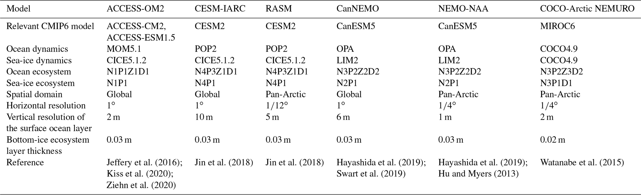
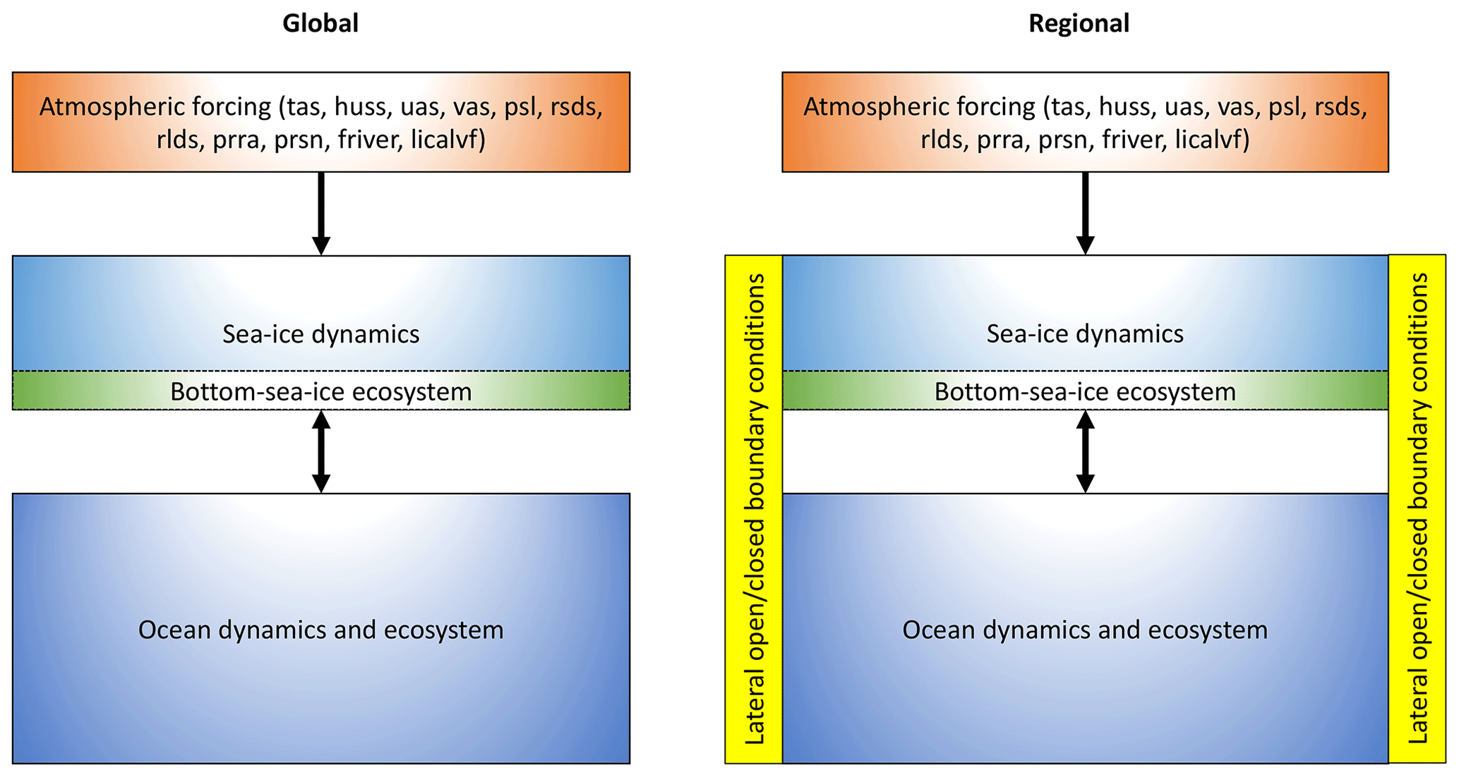
Figure 1Global (left) and regional (right) configurations of the three-dimensional coupled sea-ice–ocean physical–biogeochemical models participating in IAMIP2. The surface-atmospheric forcing dataset consists of air temperature at 10 m (tas), specific humidity at 10 m (huss), eastward wind at 10 m (uas), northward wind at 10 m (vas), sea level pressure (psl), downward shortwave radiation (rsds), downward longwave radiation (rlds), rainfall flux (prra), snowfall flux (prsn), river runoff (friver), and calving flux (licalvf).
2.1 ACCESS-OM2
ACCESS-OM2 refers to the sea-ice–ocean model of the Australian Community Climate Earth System Simulator (ACCESS) and is described in detail in Kiss et al. (2020). In brief, ACCESS-OM2 consists of an ocean dynamics component based on the Modular Ocean Model (MOM) version 5.1 and a sea-ice dynamics component based on the Los Alamos sea ice model (CICE) version 5.1.2. Notably, these sea-ice–ocean physical model components are identical to those adopted for ACCESS-CM2, the GCM of ACCESS contributing to CMIP6 (Bi et al., 2020).
For IAMIP2, ocean and sea-ice ecosystem components are added to ACCESS-OM2. The ocean ecosystem component is the Whole Ocean Model of Biogeochemistry and Trophic-dynamics (WOMBAT), which consists of nitrate, iron, phytoplankton, zooplankton, detritus, dissolved oxygen, dissolved inorganic carbon, total alkalinity, and calcium carbonate (Ziehn et al., 2020). The sea-ice ecosystem component is the Biogeochemistry of CICE (Jeffery et al., 2016), which is based on Jin et al. (2006). For IAMIP2, ACCESS-OM2 simulates ice algae biomass and nitrate concentration in the bottom-ice layer, which are coupled to phytoplankton biomass and nitrate concentration in the ocean surface layer, respectively. The horizontal resolution of ACCESS-OM2 is nominally 1∘ (360×300) and the vertical resolution in the ocean surface layer is 2.3 m (Kiss et al., 2020).
2.2 CESM-IARC
CESM-IARC refers to the 1∘ global sea-ice–ocean configuration of the Community Earth System Model (CESM) version 1 with a sub-grid-scale brine rejection parameterization that improves ocean mixing under sea ice (Jin et al., 2018). The ocean dynamic component of CESM-IARC is the Parallel Ocean Program (POP) version 2 and the sea-ice dynamic component is CICE version 5.1.2. The vertical resolution of the ocean surface layer is 10 m. The ocean ecosystem component consists of multiple nutrients (nitrate, ammonium, iron, silicate, and phosphate), phytoplankton functional groups (diatoms, flagellates, and diazotrophs), a single zooplankton group, dissolved organic matter (nitrogen, carbon, iron, and phosphorus), dissolved oxygen, dissolved inorganic carbon, and total alkalinity (Moore et al., 2013). The sea-ice ecosystem component consists of nitrate, ammonium, silicate, and ice algae (Jin et al., 2006).
2.3 RASM
RASM refers to the sea-ice–ocean configuration of the Regional Arctic System Model and consists of the same physical and ecosystem model components as CESM-IARC. The spatial coverage of RASM is pan-Arctic with lateral boundaries located approximately along the 40∘ N Atlantic sector and along the 30∘ N Pacific sector (Jin et al., 2018). The vertical resolution of the ocean surface layer is 5 m.
2.4 CanNEMO
CanNEMO is the ocean component of CanESM5 (Swart et al., 2019), which is modified from version 3.4.1 of the Nucleus for European Modelling of the Ocean (NEMO; Madec and the NEMO team, 2012) and includes the Louvain-la-Neuve sea Ice Model version 2 (LIM2; Bouillon et al., 2009; Fichefet and Maqueda, 1997). The modifications include the addition of a lee wave mixing scheme based on Saenko et al. (2012) and an update to the mesoscale eddy mixing length scale (Saenko et al., 2018), as well as various parameter settings, as described in Swart et al. (2019). CanNEMO is configured on the ORCA1 tripolar grid, with a nominal grid spacing of 1∘, refining to ∘ within 20∘ of the Equator. There are 45 vertical levels, ranging from 6 m near the surface to 250 m in the abyss. In the version used here, ocean biogeochemistry is represented by the Canadian Ocean Ecosystem (CanOE) model. CanOE contains two classes of phytoplankton, zooplankton and detritus, with variable elemental () ratios in phytoplankton and fixed ratios for zooplankton and detritus, as well as prognostic carbonate chemistry, and cycles of iron, calcium carbonate, and parameterized nitrogen fixation and denitrification (Swart et al., 2019).
For IAMIP2, CanNEMO–CanOE is coupled to the Canadian Sea-Ice Biogeochemistry (CSIB) model, which consists of nitrate, ammonium, and ice algae (Hayashida et al., 2019). Modelled ice algae have a higher sensitivity to low-light conditions relative to modelled phytoplankton (Mortenson et al., 2017). When modelled ice algae are released from sea ice into seawater, they contribute partly to the large detritus pool and the seeding of large phytoplankton.
2.5 NEMO-NAA
NEMO-NAA is a pan-Arctic regional sea-ice–ocean model based on NEMO version 3.4 coupled to LIM2 (Hu and Myers, 2013). The version used here incorporates several modifications that improve the simulation of physical and biogeochemical processes in the Arctic (Hayashida et al., 2019). Specifically, these modifications include light penetration through snow and sea ice, the vertical resolution of the ocean model, river runoff of biogeochemical tracers, removal of iron dependency of phytoplankton and zooplankton, and changes to sea-ice model parameters. The horizontal grid resolution is ∘ , which ranges from 10 km near the North American coastline to 14.5 km along the northern Eurasian coastline. The vertical resolution ranges from 1 m for the upper surface layer to 255 m in the deep ocean. Similar to CanNEMO, the ecosystem component of NEMO-NAA is CSIB–CanOE.
2.6 COCO–Arctic NEMURO
COCO–Arctic NEMURO refers to a pan-Arctic regional sea-ice–ocean model developed at the Japan Agency for Marine-Earth Science and Technology (JAMSTEC; Watanabe et al., 2019). The physical model component is the Center for Climate System Research Ocean Component Model (COCO) version 4.9 (Hasumi, 2006). The sea-ice component of COCO accounts for seven-category distributions of sub-grid snow depth and ice thickness with a one-layer thermodynamic formulation (Bitz and Lipscomb, 1999; Bitz et al., 2001; Lipscomb, 2001) and the elastic–viscous–plastic rheology (Hunke and Dukowicz, 1997). The model domain covers the entire Arctic Ocean with boundaries at the North Atlantic (45∘ N) and at the Bering Strait on the Pacific side. The Bering Strait throughflow across the Pacific model boundary is prescribed by idealized seasonal cycles of temperature, salinity, and current velocity based on Woodgate et al. (2005). The model adopts the spherical coordinate system rotated by 90∘, which sets the singular points (the North and South poles of the model grid) at the Equator. The horizontal resolution of COCO–Arctic NEMURO is ∘ , and there are 28 vertical levels in the ocean with variable resolutions from 2 m in the uppermost layer to 500 m below 1000 m depth. The ecosystem model component is the Arctic and North Pacific Ecosystem Model for Understanding Regional Oceanography (Arctic NEMURO; Watanabe et al., 2015). The ocean ecosystem model component consists of three nutrients (nitrate, ammonium, and silicate), five plankton types (diatoms, flagellates, microzooplankton, copepod, and predator zooplankton), dissolved organic nitrogen, particulate organic nitrogen, and opal (Kishi et al., 2007). The sea-ice ecosystem model component consists of ice algae, ice-related fauna, and particulate organic matter (Watanabe et al., 2015).
The experimental design of IAMIP2 is developed based on the experience from IAMIP1 and the Ocean Model Intercomparison Project (OMIP; Griffies et al., 2016; Orr et al., 2017), which is an endorsed Model Intercomparison Project (MIP) of CMIP6. The OMIP protocol is useful because OMIP is based on sea-ice–ocean models driven by common atmospheric forcing fields at their surface boundaries. Applying common forcing eliminates uncertainties due to atmospheric processes and feedbacks and allows us to focus on differences in the sea-ice, ocean, and biogeochemistry components.
Four numerical experiments are planned for IAMIP2: historical, projection, exclusion, and control as described in detail below and shown in Fig. 2. The IAMIP2 models are expected to conduct all these experiments.

Figure 2Timeline of the numerical experiments of IAMIP2. Years begin on January 1. Each experiment starts on 1 January and ends on 31 December . For example, the historical experiment starts from 1 January 1958 and ends on 31 December 2018.
3.1 Historical
The historical experiment is designed to simulate changes in ice algae abundance and distribution since the mid-20th century, the period for which we have realistic surface-atmospheric conditions based on observations. This experiment spans the 61 years from 1 January 1958 to 31 December 2018 and uses the Japanese 55-year atmospheric reanalysis for driving sea-ice–ocean models version 1.4.0, referred to here as JRA55-do (Tsujino et al., 2018). For reference, version 1.4.0 is also used for the second phase of OMIP (Tsujino et al., 2020). JRA55-do is regarded as a successor of the Coordinated Ocean-ice Reference Experiment version 2 forcing dataset (CORE2; Large and Yeager, 2009) and has finer spatial and temporal resolutions than CORE2. The surface atmospheric variables of JRA55-do are air temperature at 10 m, specific humidity at 10 m, eastward wind at 10 m, northward wind at 10 m, sea level pressure, downward shortwave radiation, downward longwave radiation, rainfall flux, snowfall flux, river runoff, and calving flux (Fig. 1). The original spatial and temporal resolutions of these variables are, respectively, ∼ 0.5∘ and 3 hourly except for river runoff and calving flux, which are provided at 0.25∘ and daily (Tsujino et al., 2018). However, in reality, the daily calving flux is provided by linear interpolation of monthly data for Greenland and it is temporally constant for Antarctica (Tsujino et al., 2018). Although JRA55-do provides calving flux, none of the IAMIP2 models have iceberg components, and therefore calving flux is released into the ocean as meltwater, adopting the approach before version 1.4.0 (Tsujino et al., 2018). JRA55-do is interpolated to the model grid either prior to or during the experiment.
All IAMIP2 models are initialized from rest (three-dimensional oceanic velocity fields and two-dimensional sea level fields are all set to zero in the first time step) and with ocean temperature, salinity, dissolved oxygen, and nutrients (nitrate, phosphate, and silicate) from the World Ocean Atlas version 2 (WOA13v2; Garcia et al., 2013; Locarnini et al., 2013; Zweng et al., 2013). More specifically, these fields are the version of WOA13v2 provided for OMIP (Griffies et al., 2016; Orr et al., 2017). There is no recommended protocol for the initialization of sea-ice and other biogeochemical fields. As discussed in Sect. 2.3 of Griffies et al. (2016), the restoring of sea-surface salinity is necessary to reduce drift in sea-ice–ocean models over decadal timescales. However, there is no best practice for salinity restoring because it depends on model details. Therefore, the restoring procedure is left to the discretion of the participating groups, although it is recommended to choose a weak restoring as much as possible to minimize the impact on variability.
Three of the IAMIP2 models are based on pan-Arctic regional configurations that require lateral boundary conditions. How to prescribe these conditions is left to the discretion of the participating groups.
Although carbonate chemistry is not the primary focus of IAMIP2, we recommend that modelled total alkalinity and dissolved inorganic carbon should be initialized with the Global Ocean Data Analysis Project version 2 (GLODAPv2; Lauvset et al., 2016) and prescribe the monthly global-mean atmospheric carbon dioxide concentration for the air–sea carbon flux (Meinshausen et al., 2017). These procedures are consistent with OMIP (Orr et al., 2017) and allow us to expand the use of the IAMIP2 product for future research.
3.2 Projection
The projection experiments are designed to simulate the projected changes in ice algae abundance and distribution throughout the 21st century under two of the greenhouse gas emission scenarios for CMIP6, known as the Shared Socioeconomic Pathways 1-2.6 and 5-8.5 (SSP1-2.6 and SSP5-8.5; O'Neill et al., 2016). SSP1-2.6 is a low-emission scenario that informs the Paris Agreement goal of limiting global warming to below 2 ∘C of the pre-industrial level. SSP5-8.5 is the highest emission scenario of CMIP6. Therefore, conducting these projections allows us to assess and compare between the impacts of strong mitigation and fossil-fuelled development (O'Neill et al., 2016). Each of these experiments spans 86 years from 2015 to 2100. The IAMIP2 models are initialized from states at the end of 2014 in the historical experiment. The atmospheric carbon dioxide concentrations are set to their monthly global-mean values prescribed for their respective SSP (Meinshausen et al., 2020).
3.2.1 Selection of the projected atmospheric forcing dataset
The IAMIP2 models are driven by the atmospheric output of selected CMIP6 models that provide the atmospheric forcing fields at the nominal spatial resolution of 100 km and at the temporal resolutions needed for simulating high-frequency (e.g., daily) variability (Holdsworth and Myers, 2015; Lebeaupin Brossier et al., 2012). To date, there are four CMIP6 models that satisfy these criteria: CMCC-CM2-SR5, CMCC-ESM2, EC-Earth3, and MRI-ESM2-0. Specifically, these models provide the simulated atmospheric forcing variables over 2015–2100 under both SSP1-2.6 and SSP5-8.5 at the temporal resolutions identical to those of JRA55-do except for sea level pressure, river runoff, and calving flux. Sea level pressure fields are provided 6 hourly as opposed to 3 hourly in JRA55-do. River runoff fields are provided at monthly as opposed to daily frequency in JRA55-do. Calving flux fields are not provided at all under any of the SSP scenarios. To partly overcome this limitation, we prescribe a monthly climatology of the calving flux of JRA55-do over 1958–2018 for the projection experiment. This will provide interannually invariant calving flux for Greenland and constant calving flux for Antarctica as noted in Sect. 3.1.
Among the four CMIP6 models, we choose the output of CMCC-ESM2 and EC-Earth3 for the atmospheric forcing for the projection experiments because CMCC-ESM2 and EC-Earth3 provide overall the most realistic atmospheric conditions (in best agreement with JRA55-do) for the south and north polar oceans, respectively. Specifically, we compare the global and polar surface air temperature and major climate modes derived from JRA55-do with those simulated by the following 26 CMIP6 models over 1958–2100 (Figs. 3 and 4): ACCESS-CM2, ACCESS-ESM1-5, AWI-CM-1-1-MR, BCC-CSM2-MR, CESM2-WACCM, CIESM, CMCC-CM2-SR5, CMCC-ESM2, CanESM5, EC-Earth3, EC-Earth3-Veg, FGOALS-f3-L, FGOALS-g3, FIO-ESM-2-0, GFDL-ESM4, INM-CM4-8, INM-CM5-0, IPSL-CM6A-LR, KACE-1-0-G, MIROC6, MPI-ESM1-2-HR, MPI-ESM1-2-LR, MRI-ESM2-0, NESM3, NorESM2-LM, and NorESM2-MM. Although the objective here is to compare among the four candidates for the projected atmospheric forcing, we include the remaining 22 CMIP6 models that have provided the output at monthly resolution as well as the multi-model mean product of the 26 models for reference. These model products belong to Variant Label r1i1p1f1 of Experiment IDs historical and ssp585, and they were downloaded from https://esgf-node.llnl.gov/ (last access: 15 July 2021).
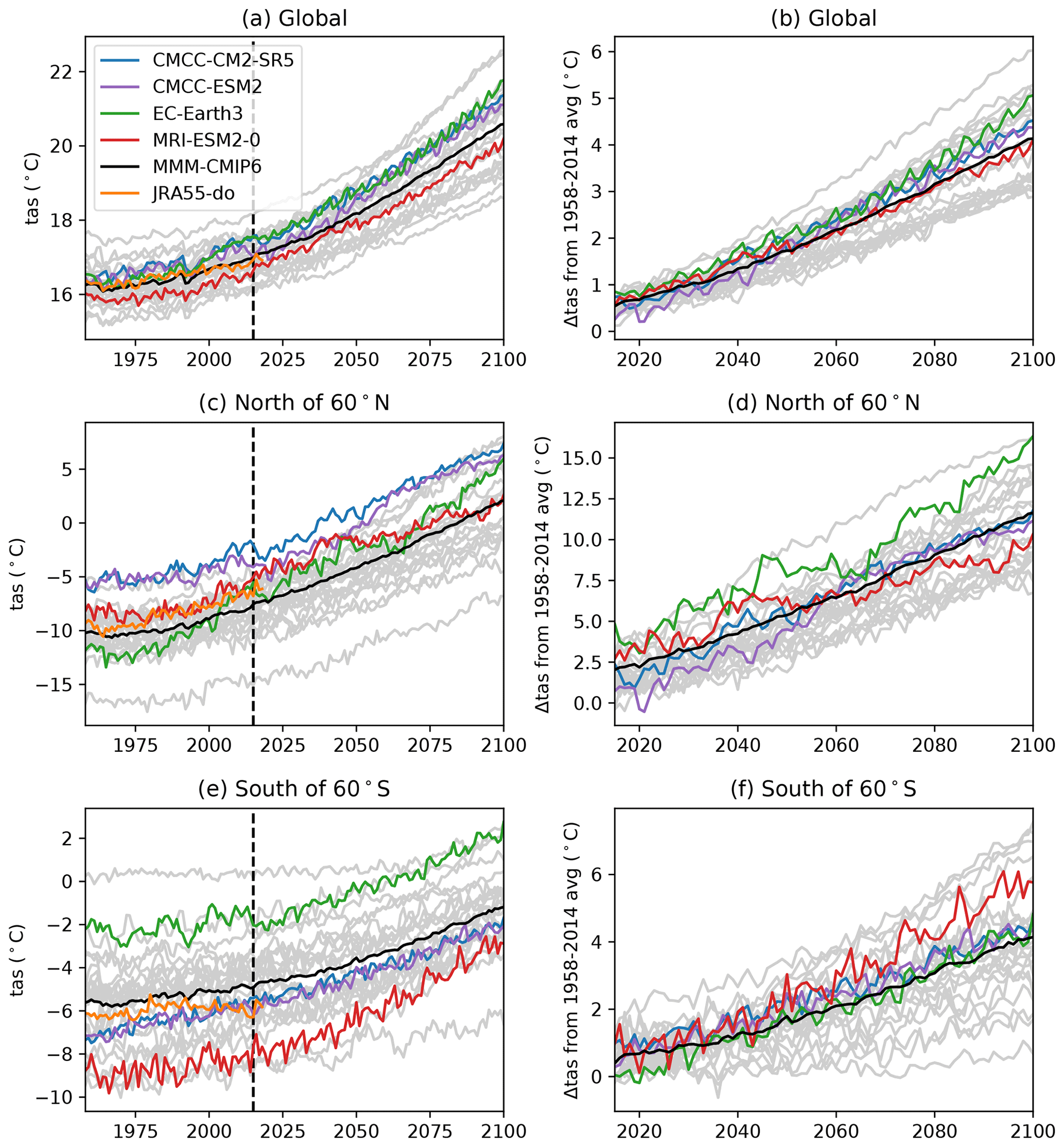
Figure 3Comparisons of historical and projected global and polar warming simulated by 26 CMIP6 models over the historical period (1958–2014) and the projection period under the SSP5-8.5 scenario (2015–2100). Time series of annual mean surface air temperature averaged over the ocean grid cells of (a) the globe, (c) the Northern Hemisphere north of 60∘ N, and (e) the Southern Hemisphere south of 60∘ S. Projected changes in annual mean surface air temperature averaged over the ocean grid cells of (b) the globe, (d) the Northern Hemisphere north of 60∘ N, and (f) the Southern Hemisphere south of 60∘ S, relative to their averages during 1958–2014. Blue, purple, green, and red denote 4 of the 26 models that provide the atmospheric output at the temporal resolutions needed for the projection experiments of IAMIP2. Grey denotes the remaining 22 models. Black denotes the multi-model mean of the 26 models. Orange denotes the JRA55-do dataset used for the atmospheric forcing for the historical experiment of IAMIP2.
3.2.2 Comparison of surface air temperature over the ocean
Surface air temperatures are averaged over the ocean grid cells globally, north of 60∘ N, and south of 60∘ S (Fig. 3). In terms of global averages, EC-Earth3 simulates surface air temperature closest to JRA55-do prior to 2000 (Fig. 3a). After 2000, EC-Earth3 simulates warmer surface air temperature that agrees well with CMCC-CM2-SR5 but deviates from JRA55-do. At the beginning of the SSP projections (2015), the global average of CMCC-ESM2 matches well with JRA55-do. MRI-ESM2-0 consistently underestimates the global averages. Compared with the multi-model averages, EC-Earth3 projects greater global warming especially in the latter half of the 21st century, whereas the MRI-ESM2-0 projection is close to the multi-model averages (Fig. 3b).
In terms of Arctic averages, MRI-ESM2-0 simulates surface air temperature that is in closest agreement with JRA55-do, but EC-Earth3 compares well later in the 2010s (Fig. 3c). In 2015, EC-Earth3 is closest to JRA55-do among the four candidates. Polar amplification is evident in all models but is more so in EC-Earth3 (>15 ∘C warming by the end of the 21st century relative to the 1958–2014 average; Fig. 3d).
In the Antarctic, the average air temperatures of CMCC-CM2-SR5 and CMCC-ESM2 agree by far the best with JRA55-do compared to the other two candidates (Fig. 3e). EC-Earth3 simulates roughly 4 ∘C warmer than JRA55-do, whereas MRI-ESM2-0 simulates approximately 3 ∘C colder surface air over the south polar ocean. MRI-ESM2-0 exhibits greater interannual variability throughout the 21st century and the greatest Antarctic warming among the four candidates (approximately 5 ∘C warming by 2100 relative to the 1958–2014 average; Fig. 3f).
3.2.3 Comparison of major climate modes of variability
Three major modes of climate variability considered here are the El Niño–Southern Oscillation (ENSO), the Northern Annular Mode (NAM), and the Southern Annular Mode (SAM). ENSO is the dominant mode of climate variability for the globe, which can be characterized by an index called the Equatorial Southern Oscillation Index (EQSOI; Bell and Halpert, 1998). EQSOI is the standardized sea level pressure difference between two regions over Indonesia (5∘ S–5∘ N, 80–130∘ W) and the eastern equatorial Pacific (5∘ S–5∘ N, 90–140∘ E). Because the CMIP6 models have their own ENSO variability, EQSOIs of these models are not expected to be in phase with that of JRA55-do (this is applicable also to other modes of climate variability, such as NAM and SAM discussed below). Instead, we compare the magnitude of the sea level pressure difference, which determines the strength of the easterly winds along the Equator (Fig. 4a). Furthermore, we compare the power spectra of EQSOI over 1958–2014 (Fig. 4b).
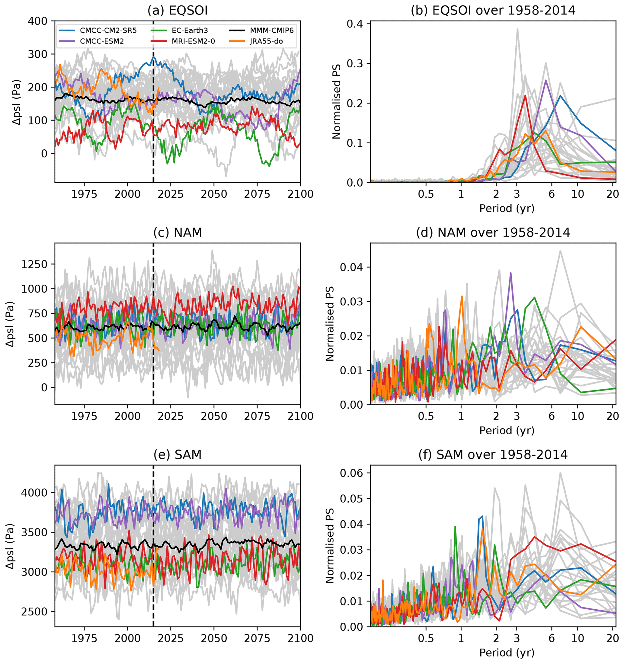
Figure 4Comparisons of major climate modes simulated by 26 CMIP6 models over the historical period (1958–2014) and the projection period under the SSP5-8.5 scenario (2015–2100). Time series of annual mean sea level pressure difference between two regions representative of (a) EQSOI, (c) NAM, and (e) SAM. Normalized power spectra of (b) EQSOI, (d) NAM, and (f) SAM derived from time series of standardized monthly mean anomaly of sea level pressure difference over 1958–2014 based on Welch's method (Welch, 1967). Blue, purple, green, and red denote 4 of the 24 models that provide the atmospheric output at the temporal resolutions needed for the projection experiment of IAMIP2. Grey denotes the remaining 22 models. Black denotes the multi-model mean of the 26 models. Orange denotes the JRA55-do dataset used for the atmospheric forcing for the historical experiment of IAMIP2.
CMCC-CM2-SR5 and CMCC-ESM2 simulate the sea level pressure difference for EQSOI that is in closer agreement with JRA55-do than the other two candidates, whose sea level pressure difference is about 100 Pa lower than JRA55-do (Fig. 4a). JRA55-do shows two maxima in the spectrum of EQSOI at periods between 3 and 6 years (Fig. 4b). MRI-ESM2-0 captures the one of these maxima at a period of about 3–4 years, while CMCC-ESM2 exhibits the other maximum at about 5–6 years. EC-Earth3 shows a maximum at a period of 4–5 years. In contrast, the EQSOI signal of CMCC-CM2-SR5 peaks at a longer period of 7–8 years.
NAM is the dominant mode of climate variability in the Northern Hemisphere, which can be characterized by the sea level pressure difference between the zonal means at 35 and 65∘ N (Li and Wang, 2003). JRA55-do overall exhibits smaller sea level pressure difference than any of the four candidates or the multi-model averages (Fig. 4c). MRI-ESM2-0 simulates somewhat larger sea level pressure difference than the other three candidates that are close to the multi-model averages. The power spectra of NAM are noisier at higher frequency (<1 year) and the peaks are spread more broadly than those of EQSOI among the candidates and JRA55-do (Fig. 4d). JRA55-do shows peaks at about 0.5, 1, and 10 years, indicating the importance of seasonal, interannual, and interdecadal variability of NAM, respectively. The four candidates also exhibit peaks within this seasonal-to-interdecadal timescale but differ in terms of the exact locations of these peaks. The strongest signal of NAM is present at a period of roughly 0.5–1 year (MRI-ESM2-0), 3 years (CMCC-CM2-SR5 and CMCC-ESM2), and 4–5 years (EC-Earth3).
SAM is the dominant mode of climate variability in the Southern Hemisphere, which can be characterized by the sea level pressure difference between the zonal means at 40 and 65∘ S (Gong and Wang, 1999). EC-Earth3 and MRI-ESM2-0 compare equally well with JRA55-do in simulating the sea level pressure difference for SAM, which is lower than the multi-model mean of the 26 CMIP6 models (Fig. 4e). In contrast, CMCC-CM2-SR5 and CMCC-ESM2 simulate about 500 Pa greater sea level pressure difference than JRA55-do. Similar to NAM, the power spectra of SAM are distributed across the broad timescales, but the peaks occur at periods of about 1 year or greater (Fig. 4f). The only exception is EC-Earth3, in which the strongest signal is present at a period of slightly less than 1 year. CMCC-CM2-SR5 agrees well with JRA55-do in simulating the absolute maximum at a period of 1–2 years. Consistent among the four candidates and JRA55-do, SAM exhibits appreciable variability also at lower frequencies, as indicated by the presence of local maxima at periods of 3–6 years and beyond 10 years. Notably, this low-frequency variability is the strongest signature of SAM simulated by MRI-ESM2-0.
3.2.4 Recommendations for the projected atmospheric forcing dataset
In summary, all four candidates for the projected atmospheric forcing dataset simulate reasonable historical atmospheric conditions compared to JRA55-do. An exception is the substantially colder surface air temperature over the Antarctic oceanic region (Fig. 3e), for which CMCC-CM2-SR5 and CMCC-ESM2 are superior to the other two models. In contrast, the latter two models outperform the former in simulating surface air temperature over the Arctic oceanic region (Fig. 3c). Therefore, there is no single candidate that does a better job than the others at both poles. For this reason, we adopt the output of two models – CMCC-ESM2-0 and EC-Earth3 – as the standard atmospheric forcing dataset for the projection experiments of IAMIP2. With two SSP scenarios, there are four combinations (CMCC-ESM2-0 ssp126, CMCC-ESM2-0 ssp585, EC-Earth3 ssp126, and EC-Earth3 ssp585; Table 2). We encourage the IAMIP2 participants to perform all the four projections. However, if computational resources are limited to undertaking only one projection, we request one of the SSP5-8.5 projections: either CMCC-ESM2-0 ssp858 (for Antarctic-focused models) or EC-Earth3 ssp585 (for Arctic-focused models). Depending on computational resources, additional projection experiments using the output of the other two candidates as well as other CMIP6 models may be considered if they provide the output at high temporal resolution. Such additional experiments will allow an assessment of the sensitivity of the IAMIP2 models to projected atmospheric conditions.
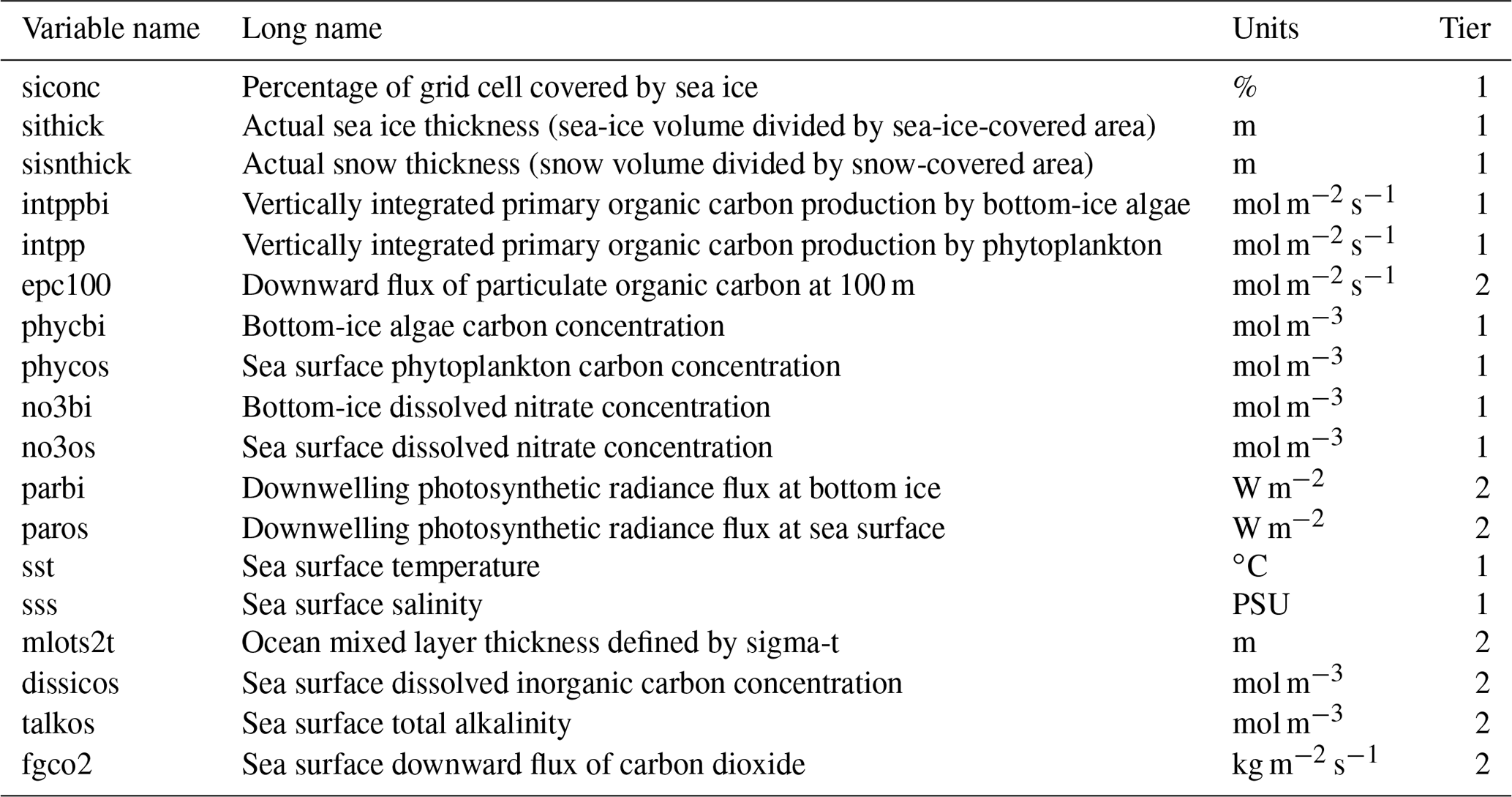
Table 2List of model diagnostics for IAMIP2. Where applicable, variable names and units follow the CMIP6 convention (https://cmip6dr.github.io/Data_Request_Home last access: 2 November 2021). Tiers refer to mandatory (Tier 1) and optional (Tier 2).
3.3 Exclusion
The exclusion experiment is designed to simulate ocean biogeochemistry in the absence of ice algae, which is the case for all CMIP6 models. This experiment is done in the same set-up as the historical experiment except that the sea-ice ecosystem component is excluded. Comparing the results of the historical and exclusion experiments allows us to quantify the impacts of ice algae on polar marine lower trophic-level ecosystems and the biological carbon pump. Doing so assesses the significance of incorporating sea-ice ecosystem components into the next-generation ESMs.
3.4 Control
The control experiment is designed to diagnose artificial model drifts and to distinguish anthropogenic effects from natural variability. This experiment spans 143 years by repeating the annual cycle of JRA55-do from 1 May 1990 to 30 April 1991, during which major climate modes were all in neutral phases (Stewart et al., 2020).
The following guidelines are developed for IAMIP2 in order to implement the Findability, Accessibility, Interoperability, and Reusability (FAIR) data principles (Wilkinson et al., 2016) and ensure that the IAMIP2 product reaches the end users (Objective 5). Specifically, we make the product discoverable from the website http://cosima.org.au/index.php/working-groups/iamip2 (last access: 2 November 2021) which provides a list of hyperlinks to the IAMIP2 product archived by individual modelling groups.
All model diagnostics are saved as daily averages in the NetCDF format, and, where applicable, their names must follow the CMIP6 naming conventions (Table 2). Daily temporal resolution is needed to quantify the bloom phenology (Watanabe et al., 2019) and to provide the ocean and sea-ice climate data for driving sea-ice biogeochemical models (Lavoie et al., 2010; Tedesco et al., 2019). To limit data storage needs, only two-dimensional fields are saved, and to preserve the spatial details in regional models, they are stored on the models' native grids. To perform interpolation for analysis, an additional file containing longitude, latitude, and grid-cell area needs to be provided for each model. The output should be stored using a common format for directory and file names (Fig. 5).

Figure 5An example file tree diagram for the IAMIP2 output. Blue denotes the directories and white denotes files. A grid file (e.g., ACCESS-OM2_grid.nc) must be provided and placed under the model directory (e.g., IAMIP2/ACCESS-OM2/). Each diagnostic file (e.g., siconc_day_IAMIP2_ACCESS-OM2_ssp585_ EC-Earth3_2015.nc) contains the output of a variable for a year.
A few examples of the potential use of these diagnostics for investigating various roles of ice algae are illustrated here. Their ecological role as the foundation of the polar marine food web and their relative importance can be quantified by comparing the biomass (phycbi and phycos; Table 2) and primary productivity between ice algae and phytoplankton (intppbi and intpp). The latter quantities can also be used to quantify the biogeochemical role of ice algae in carbon fixation and their contribution to the biological carbon pump can be assessed using particulate organic carbon export (epc100). A combination of physical (siconc, paros, sst, and mlots2t) and biogeochemical diagnostics (no3os and phyos) can be used to estimate dimethyl sulfide concentration (e.g., Bock et al., 2021; Galí et al., 2019) as well as its emission using the wind speed, which is available as the atmospheric forcing fields (uas and vas; Fig. 1).
Although the experimental design of IAMIP2 advances from that of IAMIP1 (Watanabe et al., 2019) in many aspects, it has its own limitations, which are discussed here to help the interpretation of results and for consideration by prospective end users. First, the vertical extent of the sea-ice ecosystem component of the currently committed selection of IAMIP2 models is restricted to the bottom-ice layer, which likely underestimates depth-integrated ice algae biomass and primary production because ice algae are present throughout the sea-ice column especially in the Antarctic. Although simulating ice algae throughout the sea-ice column is desirable and has been conducted under one-dimensional settings (Duarte et al., 2015; Pogson et al., 2011) as well as in a recent study using an ESM (Jeffery et al., 2020), its implementation into high-resolution three-dimensional models is computationally expensive. We anticipate that this limitation has a negligible effect on the estimation of depth-integrated biomass and primary production in landfast sea ice (Meiners et al., 2018), but it could underestimate these quantities substantially for pack ice as demonstrated by field observations (Meiners et al., 2012). We consider this a necessary compromise in order to progress IAMIP2 with currently available computational resources.
For projections of sea-ice–ocean models, a few previous studies have prescribed a synthetic atmospheric forcing dataset instead of applying the raw output of climate models in order to ensure that there is no undesirable step change in the atmospheric conditions at the beginning of projections (Naughten et al., 2018) and that the high-frequency climate variability is simulated realistically (Zhang et al., 2017). In contrast to the approach taken by these previous studies, the IAMIP2 models are driven by the raw output of CMIP6 model projections, which is made possible thanks to four CMIP6 models so far that have provided their atmospheric output available at the temporal resolutions needed to simulate the high-frequency climate variability (Holdsworth and Myers, 2015; Lebeaupin Brossier et al., 2012). Our approach is advantageous over that of the previous studies in that the IAMIP2 model projections account for projected changes in both the high- and low-frequency climate variability. As demonstrated in Sect. 3.2, there appears to be no single CMIP6 model that outperforms the other models considered here in simulating surface air temperature in both marine polar regions. Some models are better at simulating Arctic surface air temperature but not the Antarctic and vice versa. Considering this finding, we aim to perform multiple projections by prescribing the atmospheric output of two CMIP6 models (EC-Earth3 and CMCC-ESM2) under two emission scenarios (SSP1-2.6 and SSP5-8.5). To a certain extent, these projections will allow us to investigate the uncertainty in the projected changes in ice algae abundance and distribution due to the uncertainty in the projected atmospheric conditions under the same climate change scenarios. Furthermore, the implications of climate change scenarios for polar marine ecosystems and biogeochemistry can be addressed by comparison of the SSP1-2.6 and SSP5-8.5 projections.
One important source of biases in IAMIP2 projections by regional models is the lateral boundary conditions for nutrients. As a limiting factor for primary production in sea ice, prescribing the temporally varying nutrient boundary conditions is desirable. However, this is not an easy task given the large uncertainty in projected changes in nutrients especially in polar regions (e.g., Lannuzel et al., 2020).
IAMIP2 is an ongoing international effort aiming primarily to understand the role of ice algae in polar marine ecosystems and biogeochemistry at the regional and hemispheric scales. This paper describes the design of IAMIP2 which is built upon the experience from IAMIP1 (Watanabe et al., 2019) and by keeping up to date with the CMIP6 protocols (Griffies et al., 2016; O'Neill et al., 2016; Orr et al., 2017). Six three-dimensional regional and global coupled sea-ice–ocean models are currently committed to participating in IAMIP2. These models are driven by the same initial conditions and atmospheric forcing dataset to assess systematic biases in these models in terms of simulating ice algae abundance and distribution. Five numerical experiments are designed to understand the past changes since the mid-20th century by applying realistic atmospheric forcing (JRA55-do) as well as the projected changes throughout the 21st century by applying the high temporal-resolution output of selected CMIP6 model projections under the SSP1-2.6 and SSP5-8.5 scenarios. Two other experiments are used to separate the anthropogenic effect from natural variability and quantify the large-scale impacts of incorporating ice algae into regional and global models on polar marine ecosystems and biogeochemistry. The model data products of IAMIP2 are expected to meet the FAIR data principles and are intended to be used for future research and as educational tools. In conclusion, IAMIP2 is expected to advance the science of polar marine ecosystems and biogeochemistry.
The model output of IAMIP2 will be made available by individual modelling groups, which will be discoverable from the website http://cosima.org.au/index.php/working-groups/iamip2 (COSIMA, 2021). The atmospheric forcing datasets for the four projection experiments are available on the National Computational Infrastructure (NCI) National Research Data Collection (https://doi.org/10.25914/611f4e2a27300, https://doi.org/10.25914/606edd5d96a88 and https://doi.org/10.5281/zenodo.5140591) (Hayashida, 2021a, b and c). The scripts used for postprocessing CMIP6 data and plotting Figs. 3 and 4 are available in Hayashida (2021d) (https://doi.org/10.5281/zenodo.5637381).
HH conceived IAMIP2 and developed the details with MJ, NSS, NCS, and EW. AH, AK, RM, and PS supervised the ACCESS-OM2 contribution to IAMIP2. RF and HH developed the model code for enabling sea-ice–ocean coupling of biogeochemistry in ACCESS-OM2. HH prepared the projected atmospheric forcing datasets, performed the analysis, and wrote the paper with input from all co-authors.
The contact author has declared that neither they nor their co-authors have any competing interests.
Publisher’s note: Copernicus Publications remains neutral with regard to jurisdictional claims in published maps and institutional affiliations.
Hakase Hayashida thanks the members of the Consortium for Ocean-Sea Ice Modelling in Australia (COSIMA) for discussion on the atmospheric forcing dataset for future projections. This dataset is made available through technical support from Paola Petrelli from the CMS team of the Australian Research Council Centre of Excellence for Climate Extremes (CLEX). This study was undertaken with the assistance of resources and services from the NCI, which is supported by the Australian Government. Analyses are performed using the Climate Data Operator (CDO) software (Schulzweida, 2020) and Python. Normalized power spectra are computed using SciPy (Virtanen et al., 2020). Nadja S. Steiner and Neil C. Swart acknowledge funding through the Departments of Environment and Climate Change Canada and Fisheries and Oceans Canada. This work is a contribution to the Biogeochemical Exchange Processes at Sea Ice Interfaces (BEPSII) network.
This research has been supported by the Australian Research Council (grant no. CE170100023), the Grant-in-Aid for Scientific Research of the Japan Society for the Promotion of Science (JSPS) (grant no. KAKENHI 18H03368), and the Arctic Challenge for Sustainability II (ArCS II) project (grant no. JPMXD1420318865).
This paper was edited by Sandra Arndt and reviewed by three anonymous referees.
Bell, G. D. and Halpert, M. S.: Climate Assessment for 1997, Bull. Am. Meteorol. Soc., 79, S1–S50, 1998.
Bi, D., Dix, M., Marsland, S., O'Farrell, S., Sullivan, A., Bodman, R., Law, R., Harman, I., Srbinovsky, J., Rashid, H., Dobrohotoff, P., Mackallah C., Yan, H., Hirst, A., Savita, A., Dias, F. B., Woodhouse, M., Fiedler, R., and Heerdegen A.: Configuration and spin-up of ACCESS-CM2, the new generation Australian Community Climate and Earth System Simulator Coupled Model, J. South. Hemisphere Earth Syst. Sci. Submitt., 70, 225–251, https://doi.org/10.1071/ES19040, 2020.
Bitz, C. M. and Lipscomb, W. H.: An energy-conserving thermodynamic model of sea ice, J. Geophys. Res.-Oceans, 104, 15669–15677, 1999.
Bitz, C. M., Holland, M. M., Weaver, A. J., and Eby, M.: Simulating the ice-thickness distribution in a coupled climate model, J. Geophys. Res.-Oceans, 106, 2441–2463, 2001.
Bock, J., Michou, M., Nabat, P., Abe, M., Mulcahy, J. P., Olivié, D. J. L., Schwinger, J., Suntharalingam, P., Tjiputra, J., van Hulten, M., Watanabe, M., Yool, A., and Séférian, R.: Evaluation of ocean dimethylsulfide concentration and emission in CMIP6 models, Biogeosciences, 18, 3823–3860, https://doi.org/10.5194/bg-18-3823-2021, 2021.
Bouillon, S., Maqueda, M. A. M., Legat, V., and Fichefet, T.: An elastic–viscous–plastic sea ice model formulated on Arakawa B and C grids, Ocean Model, 27, 174–184, 2009.
Castellani, G., Schaafsma, F. L., Arndt, S., Lange, B. A., Peeken, I., Ehrlich, J., David, C., Ricker, R., Krumpen, T., Hendricks, S., et al., Large-Scale Variability of Physical and Biological Sea-Ice Properties in Polar Oceans, Front. Mar. Sci., 7, 536 https://doi.org/10.3389/fmars.2020.00536, 2020.
Cavan, E. L., Belcher, A., Atkinson, A., Hill, S. L., Kawaguchi, S., McCormack, S., Meyer, B., Nicol, S., Ratnarajah, L., Schmidt, K., Steinberg, D. K., Tarling, G. A., and Boyd, P. W.: The importance of Antarctic krill in biogeochemical cycles, Nat. Commun., 10, 4742, https://doi.org/10.1038/s41467-019-12668-7, 2019.
Cimoli, E., Lucieer, V., Meiners, K. M., Chennu, A., Castrisios, K., Ryan, K. G., Lund-Hansen, L. C., Martin, A., Kennedy, F., and Lucieer, A.: Mapping the in situ microspatial distribution of ice algal biomass through hyperspectral imaging of sea-ice cores, Sci. Rep., 10, 21848, https://doi.org/10.1038/s41598-020-79084-6, 2020.
Consortium for Ocean-Sea Ice Modelling in Australia (COSIMA): Ice Algae Model Intercomparison Project phase 2 (IAMIP2), COSIMA [code], available at: http://cosima.org.au/index.php/working-groups/iamip2 (last access: 3 November 2021).
Darnis, G., Robert, D., Pomerleau, C., Link, H., Archambault, P., Nelson, R. J., Geoffroy, M., Tremblay, J.-É., Lovejoy, C., Ferguson, S. H., Hunt, B. P. V., and Fortier, L.: Current state and trends in Canadian Arctic marine ecosystems: II. Heterotrophic food web, pelagic-benthic coupling, and biodiversity, Clim. Change, 115, 179–205, 2012.
Duarte, P., Assmy, P., Hop, H., Spreen, G., Gerland, S., and Hudson, S. R.: The importance of vertical resolution in sea ice algae production models, J. Mar. Syst., 145, 69–90, 2015.
Eyring, V., Bony, S., Meehl, G. A., Senior, C. A., Stevens, B., Stouffer, R. J., and Taylor, K. E.: Overview of the Coupled Model Intercomparison Project Phase 6 (CMIP6) experimental design and organization, Geosci. Model Dev., 9, 1937–1958, https://doi.org/10.5194/gmd-9-1937-2016, 2016.
Fichefet, T. and Maqueda, M. A. M.: Sensitivity of a global sea ice model to the treatment of ice thermodynamics and dynamics, J. Geophys. Res.-Oceans, 102, 12609–12646, 1997.
Galí, M., Devred, E., Babin, M., and Levasseur, M.: Decadal increase in Arctic dimethylsulfide emission, P. Natl. Acad. Sci., 201904378, 116 https://doi.org/10.1073/pnas.1904378116, 2019.
Garcia, H. E., Locarnini, R. A., Boyer, T. P., Antonov, J. I., Baranova, O. K., Zweng, M. M., Reagan, J. R., Johnson, D. R., Mishonov, A. V., and Levitus, S.: World ocean atlas 2013, Dissolved inorganic nutrients (phosphate, nitrate, silicate), 4, 76, https://doi.org/10.7289/V5J67DWD, 2013.
Gong, D. and Wang, S.: Definition of Antarctic Oscillation index, Geophys. Res. Lett., 26, 459–462, 1999.
Griffies, S. M., Danabasoglu, G., Durack, P. J., Adcroft, A. J., Balaji, V., Böning, C. W., Chassignet, E. P., Curchitser, E., Deshayes, J., Drange, H., Fox-Kemper, B., Gleckler, P. J., Gregory, J. M., Haak, H., Hallberg, R. W., Heimbach, P., Hewitt, H. T., Holland, D. M., Ilyina, T., Jungclaus, J. H., Komuro, Y., Krasting, J. P., Large, W. G., Marsland, S. J., Masina, S., McDougall, T. J., Nurser, A. J. G., Orr, J. C., Pirani, A., Qiao, F., Stouffer, R. J., Taylor, K. E., Treguier, A. M., Tsujino, H., Uotila, P., Valdivieso, M., Wang, Q., Winton, M., and Yeager, S. G.: OMIP contribution to CMIP6: experimental and diagnostic protocol for the physical component of the Ocean Model Intercomparison Project, Geosci. Model Dev., 9, 3231–3296, https://doi.org/10.5194/gmd-9-3231-2016, 2016
Hasumi, H.: CCSR Ocean Component Model (COCO) version 4.0 (University of Tokyo), 111 pp, 2015, https://ccsr.aori.u-tokyo.ac.jp/~hasumi/COCO/coco4.pdf (last access date: 3 November 2021), 2006.
Hayashida, H.: EC-Earth3 SSP585 atmospheric forcing dataset for the Ice Algae Model Intercomparison Project phase 2 (IAMIP2) projection experiment v1.0, NCI National Research Data Collection [data set], https://doi.org/10.25914/606edd5d96a88, 2021a.
Hayshida, H.: Atmospheric forcing datasets for the Ice Algae Model Intercomparison Project phase 2 (IAMIP2) projection experiments v1.0, NCI National Research Data Collection [data set], https://doi.org/10.25914/611f4e2a27300, 2021b.
Hayashida H.: hakaseh/prep_iamip2_forcing: Atmospheric forcing datasets for the IAMIP2 projection experiments (4 projections) (v1.1), Zenodo, [data set], https://doi.org/10.5281/zenodo.5140591, 2021c.
Hayashida, H.: hakaseh/iamip2_cmip6_analysis: IAMIP2 protocol paper (GMD) (Version v1), Zenodo [data set], https://doi.org/10.5281/zenodo.5637381, 2021d.
Hayashida, H., Christian, J. R., Holdsworth, A. M., Hu, X., Monahan, A. H., Mortenson, E., Myers, P. G., Riche, O. G. J., Sou, T., and Steiner, N. S.: CSIB v1 (Canadian Sea-ice Biogeochemistry): a sea-ice biogeochemical model for the NEMO community ocean modelling framework, Geosci. Model Dev., 12, 1965–1990, https://doi.org/10.5194/gmd-12-1965-2019, 2019.
Holdsworth, A. M. and Myers, P. G.: The Influence of High-Frequency Atmospheric Forcing on the Circulation and Deep Convection of the Labrador Sea, J. Clim., 28, 4980–4996, 2015.
Hunke, E. C. and Dukowicz, J. K.: An elastic-viscous-plastic model for sea ice dynamics, J. Phys. Oceanogr., 27, 1849–1867, 1997.
Hu, X. and Myers, P. G.: A Lagrangian view of Pacific water inflow pathways in the Arctic Ocean during model spin-up, Ocean Model, 71, 66–80, 2013.
Jeffery, N., Elliott, S. M., Hunke, E. C., Lipscomb, W. H., and Turner, A. K.: Biogeochemistry of Cice: The Los Alamos Sea Ice Model Documentation and Software User's Manual Zbgc_ colpkg Modifications to Version 5 (Los Alamos National Lab, (LANL), Los Alamos, NM (United States)), https://doi.org/10.2172/1329842, 2016.
Jeffery, N., Maltrud, M. E., Hunke, E. C., Wang, S., Wolfe, J., Turner, A. K., Burrows, S. M., Shi, X., Lipscomb, W. H., Maslowski, W., and Calvin, K. V.: Investigating controls on sea ice algal production using E3SMv1.1-BGC, Ann. Glaciol, 61, 51–72, https://doi.org/10.1017/aog.2020.7, 2020.
Jin, M., Deal, C. J., Wang, J., Shin, K.-H., Tanaka, N., Whitledge, T. E., Lee, S. H., and Gradinger, R. R.: Controls of the landfast ice–ocean ecosystem offshore Barrow, Alaska, Ann. Glaciol., 44, 63–72, 2006.
Jin, M., Deal, C., Maslowski, W., Matrai, P., Roberts, A., Osinski, R., Lee, Y. J., Frants, M., Elliott, S., Jeffery, N., Hunke, E., Wang, S.: Effects of Model Resolution and Ocean Mixing on Forced Ice-Ocean Physical and Biogeochemical Simulations Using Global and Regional System Models, J. Geophys. Res.-Oceans, 123, 358–377, 2018.
Kishi, M. J., Kashiwai, M., Ware, D. M., Megrey, B. A., Eslinger, D. L., Werner, F. E., Noguchi-Aita, M., Azumaya, T., Fujii, M., Hashimoto, Huang, D., Iizumi, H., Ishida, Y., Kang, S., Kantakov, G. A.,Kim H., Komatsu, K., Navrotsky, V. V., Smith, S.L., Tadokoro, K., Tsuda, A., Yamamura, O., Yamanaka, Y., Yokouchi, K., Yoshie, N., Zhang, J., Zuenko, Y. I., and Zvalinsky, V. I.: NEMURO – a lower trophic level model for the North Pacific marine ecosystem, Ecol. Model., 202, 12–25, 2007.
Kiss, A. E., Hogg, A. McC., Hannah, N., Boeira Dias, F., Brassington, G. B., Chamberlain, M. A., Chapman, C., Dobrohotoff, P., Domingues, C. M., Duran, E. R., England, M. H., Fiedler, R., Griffies, S. M., Heerdegen, A., Heil, P., Holmes, R. M., Klocker, A., Marsland, S. J., Morrison, A. K., Munroe, J., Nikurashin, M., Oke, P. R., Pilo, G. S., Richet, O., Savita, A., Spence, P., Stewart, K. D., Ward, M. L., Wu, F., and Zhang, X.: ACCESS-OM2 v1.0: a global ocean–sea ice model at three resolutions, Geosci. Model Dev., 13, 401–442, https://doi.org/10.5194/gmd-13-401-2020, 2020.
Lange, B. A., Katlein, C., Castellani, G., Fernández-Méndez, M., Nicolaus, M., Peeken, I., and Flores, H.: Characterizing Spatial Variability of Ice Algal Chlorophyll a and Net Primary Production between Sea Ice Habitats Using Horizontal Profiling Platforms, Front. Mar. Sci., 4, 349, https://doi.org/10.3389/fmars.2017.00349, 2017.
Lannuzel, D., Tedesco, L., van Leeuwe, M., Campbell, K., Flores, H., Delille, B., Miller, L., Stefels, J., Assmy, P., Bowman, J., Brown, K., Castellani, G., Chierici, M., Crabeck, O., Damm, E., Else, B., Fransson, A., Fripiat, F., Geilfus, N.-X., Jacques, C., Jones, E., Kaartokallio, H., Kotovitch, H., Meiners, K., Moreau, S., Nomura, D., Peeken, I., Rintala, J.-M., Steiner, N., Tison, J.-L., Vancoppenolle, M., Van der Linden, F., Vichi, M., and Wongpan, P.: The future of Arctic sea-ice biogeochemistry and ice-associated ecosystems, Nat. Clim. Change, 10, 983–992, https://doi.org/10.1038/s41558-020-00940-4, 2020.
Large, W. G. and Yeager, S. G.: The global climatology of an interannually varying air–sea flux data set, Clim. Dyn., 33, 341–364, 2009.
Lauvset, S. K., Key, R. M., Olsen, A., van Heuven, S., Velo, A., Lin, X., Schirnick, C., Kozyr, A., Tanhua, T., Hoppema, M., Jutterström, S., Steinfeldt, R., Jeansson, E., Ishii, M., Perez, F. F., Suzuki, T., and Watelet, S.: A new global interior ocean mapped climatology: the 1° × 1° GLODAP version 2, Earth Syst. Sci. Data, 8, 325–340, https://doi.org/10.5194/essd-8-325-2016, 2016.
Lavoie, D., Denman, K. L., and Macdonald, R. W.: Effects of future climate change on primary productivity and export fluxes in the Beaufort Sea, J. Geophys. Res.-Oceans, 115, C04018, https://doi.org/10.1029/2009JC005493, 2010.
Lebeaupin Brossier, C., Béranger, K., and Drobinski, P.: Sensitivity of the northwestern Mediterranean Sea coastal and thermohaline circulations simulated by the ∘ -resolution ocean model NEMO-MED12 to the spatial and temporal resolution of atmospheric forcing, Ocean Model, 43–44, 94–107, 2012.
Leu, E., Mundy, C. J., Assmy, P., Campbell, K., Gabrielsen, T. M., Gosselin, M., Juul-Pedersen, T., and Gradinger, R.: Arctic spring awakening – Steering principles behind the phenology of vernal ice algal blooms, Prog. Oceanogr., 139, 151–170, 2015.
Levasseur, M.: Impact of Arctic meltdown on the microbial cycling of sulphur, Nat. Geosci., 6, 691–700, 2013.
Li, J. and Wang, J. X. L.: A modified zonal index and its physical sense, Geophys. Res. Lett., 30, 1632, https://doi.org/10.1029/2003GL017441, 2003.
Lipscomb, W. H.: Remapping the thickness distribution in sea ice models, J. Geophys. Res.-Oceans, 106, 13989–14000, 2001.
Locarnini, R. A., Mishonov, A. V., Antonov, J. I., Boyer, T. P., Garcia, H. E., Baranova, O. K., Zweng, M. M., Paver, C. R., Reagan, J. R., and Johnson, D. R.: World ocean atlas 2013, Temperature, 1, 73, 40 pp., https://doi.org/10.7289/V55X26VD, 2013.
Madec, G. and the NEMO team: NEMO ocean engine, version3.4 (Institut Pierre-Simon Laplace Note du Pole de Modélisation), 2012.
Meiners, K. M., Vancoppenolle, M., Thanassekos, S., Dieckmann, G. S., Thomas, D. N., Tison, J.-L., Arrigo, K. R., Garrison, D. L., McMinn, A., Lannuzel, D., Lannuzel, D., van der Merwe, P., Swadling, K. M., Smith Jr., W.O., Melnikov, I., and Raymond, B.: Chlorophyll a in Antarctic sea ice from historical ice core data, Geophys. Res. Lett., 39, L21602, https://doi.org/10.1029/2012GL053478, 2012.
Meiners, K. M., Vancoppenolle, M., Carnat, G., Castellani, G., Delille, B., Delille, D., Dieckmann, G. S., Flores, H., Fripiat, F., Grotti, Lange, B. A., Lannuzel, D., Martin A., McMinn, A., Nomura, D., Peeken, I., Rivaro, P., Ryan, K. G., Stefels, J., Swadling, K. M., Thomas, D. N., Tison, J.-L., van der Merwe, P., van Leeuwe, M. A., Weldrick, C., and Yang, E. J.: Chlorophyll-a in Antarctic Landfast Sea Ice: A First Synthesis of Historical Ice Core Data, J. Geophys. Res.-Oceans, 123, 8444–8459, 2018.
Meinshausen, M., Vogel, E., Nauels, A., Lorbacher, K., Meinshausen, N., Etheridge, D. M., Fraser, P. J., Montzka, S. A., Rayner, P. J., Trudinger, C. M., Krummel, P. B., Beyerle, U., Canadell, J. G., Daniel, J. S., Enting, I. G., Law, R. M., Lunder, C. R., O'Doherty, S., Prinn, R. G., Reimann, S., Rubino, M., Velders, G. J. M., Vollmer, M. K., Wang, R. H. J., and Weiss, R.: Historical greenhouse gas concentrations for climate modelling (CMIP6), Geosci. Model Dev., 10, 2057–2116, https://doi.org/10.5194/gmd-10-2057-2017, 2017.
Meinshausen, M., Nicholls, Z. R. J., Lewis, J., Gidden, M. J., Vogel, E., Freund, M., Beyerle, U., Gessner, C., Nauels, A., Bauer, N., Canadell, J. G., Daniel, J. S., John, A., Krummel, P. B., Luderer, G., Meinshausen, N., Montzka, S. A., Rayner, P. J., Reimann, S., Smith, S. J., van den Berg, M., Velders, G. J. M., Vollmer, M. K., and Wang, R. H. J.: The shared socio-economic pathway (SSP) greenhouse gas concentrations and their extensions to 2500, Geosci. Model Dev., 13, 3571–3605, https://doi.org/10.5194/gmd-13-3571-2020, 2020.
Miller, L. A., Fripiat, F., Else, B. G. T., Bowman, J. S., Brown, K. A., Collins, R. E., Ewert, M., Fransson, A., Gosselin, M., Lannuzel, D., Meiners, K. M., Michel, C., Nishioka, J., Nomura, D., Papadimitriou, S., Russell, L. M., Sørensen, L. L., Thomas, D. N., Tison, J.-L., van Leeuwe, M. A., Vancoppenolle, M., Wolff, E. W., and Zhou, J.: Methods for biogeochemical studies of sea ice: The state of the art, caveats, and recommendations, Elem. Sci. Anthr., 3, 000038, 53, https://doi.org/10.12952/journal.elementa.000038, 2015.
Moore, J. K., Lindsay, K., Doney, S. C., Long, M. C., and Misumi, K.: Marine Ecosystem Dynamics and Biogeochemical Cycling in the Community Earth System Model [CESM1(BGC)]: Comparison of the 1990s with the 2090s under the RCP4.5 and RCP8.5 Scenarios, J. Clim., 26, 9291–9312, 2013.
Mortenson, E., Hayashida, H., Steiner, N., Monahan, A., Blais, M., Gale, M. A., Galindo, V., Gosselin, M., Hu, X., Lavoie, D., Mundy, C. J.: A model-based analysis of physical and biological controls on ice algal and pelagic primary production in Resolute Passage, Elem. Sci. Anth., 5, 39, https://doi.org/10.1525/elementa.229, 2017.
Mortenson, E., Steiner, N., Monahan, A. H., Hayashida, H., Sou, T., and Shao, A.: Modeled Impacts of Sea Ice Exchange Processes on Arctic Ocean Carbon Uptake and Acidification (1980–2015), J. Geophys. Res.-Oceans, 125, e2019JC015782, https://doi.org/10.1029/2019JC015782, 2020.
Naughten, K. A., Meissner, K. J., Galton-Fenzi, B. K., England, M. H., Timmermann, R., and Hellmer, H. H.: Future Projections of Antarctic Ice Shelf Melting Based on CMIP5 Scenarios, J. Clim., 31, 5243–5261, 2018.
O'Neill, B. C., Tebaldi, C., van Vuuren, D. P., Eyring, V., Friedlingstein, P., Hurtt, G., Knutti, R., Kriegler, E., Lamarque, J.-F., Lowe, J., Meehl, G. A., Moss, R., Riahi, K., and Sanderson, B. M.: The Scenario Model Intercomparison Project (ScenarioMIP) for CMIP6, Geosci. Model Dev., 9, 3461–3482, https://doi.org/10.5194/gmd-9-3461-2016, 2016.
Orr, J. C., Najjar, R. G., Aumont, O., Bopp, L., Bullister, J. L., Danabasoglu, G., Doney, S. C., Dunne, J. P., Dutay, J.-C., Graven, H., Griffies, S. M., John, J. G., Joos, F., Levin, I., Lindsay, K., Matear, R. J., McKinley, G. A., Mouchet, A., Oschlies, A., Romanou, A., Schlitzer, R., Tagliabue, A., Tanhua, T., and Yool, A.: Biogeochemical protocols and diagnostics for the CMIP6 Ocean Model Intercomparison Project (OMIP), Geosci. Model Dev., 10, 2169–2199, https://doi.org/10.5194/gmd-10-2169-2017, 2017.
Pogson, L., Tremblay, B., Lavoie, D., Michel, C., and Vancoppenolle, M.: Development and validation of a one-dimensional snow-ice algae model against observations in Resolute Passage, Canadian Arctic Archipelago, J. Geophys. Res., 116, C04010, https://doi.org/10.1029/2010JC006119, 2011.
Saenko, O. A., Zhai, X., Merryfield, W. J., and Lee, W. G.: The Combined Effect of Tidally and Eddy-Driven Diapycnal Mixing on the Large-Scale Ocean Circulation, J. Phys. Oceanogr., 42, 526–538, 2012.
Saenko, O. A., Yang, D., and Gregory, J. M.: Impact of Mesoscale Eddy Transfer on Heat Uptake in an Eddy-Parameterizing Ocean Model, J. Clim., 31, 8589–8606, 2018.
Schulzweida, U.: CDO User Guide (2.0.0), Zenodo [software], https://doi.org/10.5281/zenodo.5614769, 2020.
Smith, D. M., Screen, J. A., Deser, C., Cohen, J., Fyfe, J. C., García-Serrano, J., Jung, T., Kattsov, V., Matei, D., Msadek, R., Peings, Y., Sigmond, M., Ukita, J., Yoon, J.-H., and Zhang, X.: The Polar Amplification Model Intercomparison Project (PAMIP) contribution to CMIP6: investigating the causes and consequences of polar amplification, Geosci. Model Dev., 12, 1139–1164, https://doi.org/10.5194/gmd-12-1139-2019, 2019.
Stewart, K. D., Kim, W. M., Urakawa, S., Hogg, A. McC., Yeager, S., Tsujino, H., Nakano, H., Kiss, A. E., and Danabasoglu, G.: JRA55-do-based repeat year forcing datasets for driving ocean–sea-ice models, Ocean Model, 147, 101557, https://doi.org/10.1016/j.ocemod.2019.101557 2020.
Swart, N. C., Cole, J. N. S., Kharin, V. V., Lazare, M., Scinocca, J. F., Gillett, N. P., Anstey, J., Arora, V., Christian, J. R., Hanna, S., Jiao, Y., Lee, W. G., Majaess, F., Saenko, O. A., Seiler, C., Seinen, C., Shao, A., Sigmond, M., Solheim, L., von Salzen, K., Yang, D., and Winter, B.: The Canadian Earth System Model version 5 (CanESM5.0.3), Geosci. Model Dev., 12, 4823–4873, https://doi.org/10.5194/gmd-12-4823-2019, 2019.
Tedesco, L., Vichi, M., and Scoccimarro, E.: Sea-ice algal phenology in a warmer Arctic, Sci. Adv., 5, eaav4830, https://doi.org/10.1126/sciadv.aav4830, 2019.
Tsujino, H., Urakawa, S., Nakano, H., Small, R. J., Kim, W. M., Yeager, S. G., Danabasoglu, G., Suzuki, T., Bamber, J. L., Bentsen, M., Böning, C. W., Bozec, A., Chassignet, E. P., Curchitser, E., Dias, F. B., Durack, P. J., Griffies, S. M., Harada, Y., Ilicak, M., Josey, S. A., Kobayashi C., Kobayashi, S., Komuro, Y., Large, W. G., Le Sommer, J., Marsland, S. J., Masina, S., Scheinert, M., Tomita, H., Valdivieso, M., and Yamazaki, D.: JRA-55 based surface dataset for driving ocean–sea-ice models (JRA55-do), Ocean Model, 130, 79–139, 2018.
Tsujino, H., Urakawa, L. S., Griffies, S. M., Danabasoglu, G., Adcroft, A. J., Amaral, A. E., Arsouze, T., Bentsen, M., Bernardello, R., Böning, C. W., Bozec, A., Chassignet, E. P., Danilov, S., Dussin, R., Exarchou, E., Fogli, P. G., Fox-Kemper, B., Guo, C., Ilicak, M., Iovino, D., Kim, W. M., Koldunov, N., Lapin, V., Li, Y., Lin, P., Lindsay, K., Liu, H., Long, M. C., Komuro, Y., Marsland, S. J., Masina, S., Nummelin, A., Rieck, J. K., Ruprich-Robert, Y., Scheinert, M., Sicardi, V., Sidorenko, D., Suzuki, T., Tatebe, H., Wang, Q., Yeager, S. G., and Yu, Z.: Evaluation of global ocean–sea-ice model simulations based on the experimental protocols of the Ocean Model Intercomparison Project phase 2 (OMIP-2), Geosci. Model Dev., 13, 3643–3708, https://doi.org/10.5194/gmd-13-3643-2020, 2020.
Vancoppenolle, M. and Tedesco, L.: Numerical models of sea ice biogeochemistry, in: Sea Ice, third edn., edited by: Thomas, D. N., John Wiley & Sons, Chichester, UK, https://doi.org/10.1002/9781118778371.ch20, 2017.
Virtanen, P., Gommers, R., Oliphant, T. E., Haberland, M., Reddy, T., Cournapeau, D., Burovski, E., Peterson, P., Weckesser, W., Bright, J., van der Walt, S. J., Brett, M., Wilson, J., Millman, K. J., Mayorov, N., Nelson, A. R. J., Jones, E., Kern, R., Larson, E., Carey, C. J., Polat, İ., Feng, Y., Moore, E. W., VanderPlas, J., Laxalde, D., Perktold, J., Cimrman, R., Henriksen, I., Quintero, E. A., Harris, C. R., Archibald, A. M., Ribeiro, A. H., Pedregosa, F., van Mulbregt, P., and SciPy 1.0 Contributors: fundamental algorithms for scientific computing in Python, Nat. Methods, 17, 261–272, 2020.
Watanabe, E., Onodera, J., Harada, N., Aita, M. N., Ishida, A., and Kishi, M. J.: Wind-driven interannual variability of sea ice algal production in the west ern Arctic Chukchi Borderland, Biogeosciences, 12, 6147–6168, https://doi.org/10.5194/bg-12-6147-2015, 2015.
Watanabe, E., Jin, M., Hayashida, H., Zhang, J., and Steiner, N.: Multi-Model Intercomparison of the Pan-Arctic Ice-Algal Productivity on Seasonal, Interannual, and Decadal Timescales, J. Geophys. Res.-Oceans, 124, 9053–9084, 2019.
Welch, P.: The use of fast Fourier transform for the estimation of power spectra: A method based on time averaging over short, modified periodograms, IEEE Trans. Audio Electroacoustics, 15, 70–73, 1967.
Wilkinson, M. D., Dumontier, M., Aalbersberg, I. J., Appleton, G., Axton, M., Baak, A., Blomberg, N., Boiten, J.-W., da Silva Santos, L. B., Bourne, P. E., Bouwman, J., Brookes, A. J., Clark, T. Crosas, M., Dillo, I., Dumon, O., Edmunds, S., Evelo, C. T., Finkers, R., Gonzalez-Beltran, A., Gray, A. J. G., Groth, P., Goble, C., Grethe, J. S., Heringa, J., Hoen, P. A. C., Hooft, R., Kuhn, T., Kok, R., Kok, J., Lusher, S. J., Martone, M. E., Mons, A., Packer, A. L., Persson, B., Rocca-Serra, P., Roos, M., van Schaik, R., Sansone, S.-A., Schultes, E., Sengstag, T., Slater, T., Strawn, G., Swertz, M. A., Thompson, M., van der Lei, J., van Mulligen, E., Velterop, J., Waagmeester, A., Wittenburg, P., Wolstencroft, K., Zhao, J., and Mons, B.: The FAIR Guiding Principles for scientific data management and stewardship, Sci. Data, 3, 1–9, 2016.
Woodgate, R. A., Aagaard, K., and Weingartner, T. J.: Monthly temperature, salinity, and transport variability of the Bering Strait through flow, Geophys. Res. Lett., 32, L04601, https://doi.org/10.1029/2004GL021880, 2005.
Zeebe, R. E., Eicken, H., Robinson, D. H., Wolf-Gladrow, D., and Dieckmann, G. S.: Modeling the heating and melting of sea ice through light absorption by microalgae, J. Geophys. Res.-Oceans, 101, 1163–1181, 1996.
Zhang, X., Church, J. A., Monselesan, D., and McInnes, K. L.: Sea level projections for the Australian region in the 21st century, Geophys. Res. Lett., 44, 8481–8491, 2017.
Ziehn, T., Chamberlain, M. A., Law, R. M., Lenton, A., Bodman, R. W., Dix, M., Stevens, L., Wang, Y.-P., and Srbinovsky, J.: The Australian Earth System Model: ACCESS-ESM1.5, J. South. Hemisphere, Earth Syst. Sci., 70, 193–214, https://doi.org/10.1071/ES19035, 2020.
Zweng, M. M., Reagan, J. R., Antonov, J. I., Locarnini, R. A., Mishonov, A. V., Boyer, T. P., Garcia, H. E., Baranova, O. K., Johnson, D. R., and Seidov, D.: World ocean atlas 2013, Volume 2, Salinity, edited by: Levitus, S., and Mishonov, A., Technical Ed., NOAA Atlas NESDIS; 74, https://doi.org/10.7289/V5251G4D, 2013.