Verification of boundary layer wind patterns in COSMO-REA2 using clear-air radar echoes

The verification of high-resolution meteorological models requires highly resolved validation data and appropriate tools of analysis. While much progress has been made in the case of precipitation, wind fields have received less attention, largely due to a lack of spatial measurements. Clear-sky radar echoes could be an unexpected part of the solution by affording us an indirect look at horizontal wind patterns: regions of horizontal convergence attract non-meteorological scatterers such as insects; their concentration visualizes the structure of the convergence field. Using a two-dimensional wavelet transform, this study demonstrates how divergences and reflectivities can be quantitatively compared in terms of their spatial scale, anisotropy (horizontal), and direction. A long-term validation of the highly resolved regional reanalysis COSMO-REA2 against the German radar mosaic shows surprisingly close agreement. Despite theoretically predicted problems with simulations in or near the “grey zone” of turbulence, COSMO-REA2 is shown to produce a realistic diurnal cycle of the spatial scales larger than 8 km. In agreement with the literature, the orientation of the patterns in both datasets closely follows the mean wind direction. Conversely, an analysis of the horizontal anisotropy reveals that the model has an unrealistic tendency towards highly linear, roll-like patterns early in the day.

1 Introduction

Modern numerical weather models at horizontal resolutions on the order of 1–10 km are generally believed to be useful, but their added value compared to coarser models is not easy to quantify. On the one hand, the precise placement of very small features continues to be largely unpredictable. In a comparison conducted grid point by grid point, highly resolved models are punished twice for slight location errors in features, which coarser models do not attempt to simulate at all. On the other hand, a single error value summarizing the realism of a highly complex meteorological field is not very informative. To address these issues, a large variety of so-called spatial verification techniques has been developed in recent years. A first systematic survey of the field was undertaken in the Spatial Forecast Verification Methods Intercomparison Project (Gilleland et al., 2009, ICP). At this point, almost all efforts were focused on the verification of precipitation forecasts for several reasons: firstly, the improved representation of convective precipitation was a main incentive for the development of mesoscale weather models. Secondly, the intermittent nature of rain fields makes the aforementioned double-penalty problem particularly obvious. Lastly, radar (and to a lesser degree, satellite) observations readily provide high-resolution spatial observations of precipitation.

The second phase of the ICP (Dorninger et al., 2018) has highlighted the need for a spatial verification of other meteorological variables, particularly wind: wind fields at kilometer resolutions can produce highly complex patterns with potential impacts on convective initiation, wind energy, air quality, and aviation safety. The task of verifying spatial wind forecasts poses practical, methodological, and theoretical challenges.

From a practical point of view, we face a lack of spatial observations: model analyses (e.g., used for wind verification by Zschenderlein et al., 2019) conveniently provide highly resolved, gap-free data, but the realism of the underlying model would have to be verified against some other data beforehand. Interpolated station data are generally too coarsely resolved to represent structures on the scale of a few kilometers, and denser station networks such as the WegenerNet dataset used by Schlager et al. (2019) are rare. Bousquet et al. (2008) and Beck et al. (2014) use multi-Doppler wind retrievals from the French national radar network to verify numerical wind predictions. This approach is very appealing but limited to cases with precipitation. In addition, the necessary overlap of multiple radar beams severely limits the operationally available coverage within the atmospheric boundary layer; the authors cited above therefore focus on winds at 2 km height. Lastly, multi-Doppler wind retrievals are not trivial to construct, and such datasets are not yet widely available.

Skinner et al. (2016) present a very interesting alternative using single-Doppler azimuthal wind shear as a proxy for low-level rotation. Their study also highlights some of the main methodological challenges related to wind verification: most spatial verification techniques were developed for scalar quantities that can be decomposed into discrete objects via thresholding. How should such techniques be adapted to vector fields for which nonzero variability is present at every location and the existence of well-defined objects is not guaranteed? Skinner et al. (2016), who are interested in tornado forming mesocyclones, chose to focus on the rotational component of the wind field by verifying only the horizontal vorticity. Model and observations are subjected to several spatial filters and then thresholded at manually selected values before the method for object-based diagnostic evaluation (Davis et al., 2009) and the displacement and amplitude score of Keil and Craig (2009) are applied. Their approach is justified because well-defined objects, i.e., tornadic supercells, clearly exist in the specific case study under consideration. Bousquet et al. (2008) find a similar answer to the vector problem by verifying horizontal divergences against the corresponding values from the French multi-Doppler network. Besides pointwise measures, these authors apply a simple scale-separation approach based on a Haar wavelet decomposition of the wind fields. Other recent attempts at spatial wind verification include Zschenderlein et al. (2019), who apply the object-based structure, amplitude, and location technique (Wernli et al., 2008) to thresholded predictions of gusts (i.e., absolute wind speed), and Skok and Hladnik (2018), who sort wind vectors into classes based on their speed and direction and use the popular fractions skill score (Roberts and Lean, 2008) to find the scales on which the predicted classes agree with the observations.

In this study, we take a similar route as Skinner et al. (2016), but instead of the rotational component we focus on the horizontal divergence of the boundary layer wind field. Under the right environmental conditions, the spatial pattern of this divergence field can be observed in widely available radar reflectivity data: on warm, rain-free days, convergent boundary layer circulations attract swarms of insects, which are drawn in and actively attempt to resist the vertical motion of updrafts (Wilson et al., 1994). The resulting increased concentration of biological scatterers within the radar beam reflects the pattern of convergence and divergence. Numerous studies including Weckwerth et al. (1997, 1999), Thurston et al. (2016), and Banghoff et al. (2020) have used these kinds of data to study the dominant patterns of boundary layer organization. Atkinson and Wu Zhang (1996) identified mesoscale shallow convection, organized in the form of cells or horizontal rolls, as the most prominent of those patterns. Numerous studies have used radar data to observe these phenomena (see references in Banghoff et al., 2020); Banghoff et al. (2020) also present a first long-time climatology using 10 years of reflectivities and Doppler velocities from a single radar station in Oklahoma. They manually classified radar images from over 1000 d into cells, rolls, and unorganized patterns, reporting organized features on 92 % of summer days without rain. Santellanes et al. (2021) exploited this dataset to study the environmental conditions that favor the different modes of organization.

In the present investigation, we aim to study a similarly large database of reflectivities from the German radar mosaic RADOLAN (radar online adjustment, “RADar OnLine ANeichung”) and compare it to divergence structures from COSMO-REA2 (Wahl et al., 2017). This regional reanalysis at 2 km horizontal resolution is based on the COSMO (COnsortium for Small-scale MOdeling) model and covers the time span from 2007 to 2013. We limit our analysis to small environments around each radar station and consider both the entire COSMO-REA2 time series (for an overall model climatology) and the subset for which clear-air radar echoes are available (for verification).

For a fair, quantitative validation of the model, the spatial patterns must be analyzed objectively. Here, we rely on the wavelet-based scale, anisotropy, and direction (SAD) verification methodology of Buschow and Friederichs (2021), which applies a series of directed filters to objectively determine the dominant spatial scale, anisotropy, and direction in an image. A closely related approach was used to define a wavelet-based index of convective organization in radar and satellite images by Brune et al. (2021).

To what extent a model at 𝒪(1 km) horizontal resolution can be expected to realistically represent boundary layer circulations in the so-called “grey zone” regime (Wyngaard, 2004) between parameterized and resolved turbulence is a difficult question that poses further theoretical challenges to the verification process. Section 2 therefore briefly summarizes some of the relevant theoretical and experimental results from the literature. Data and methodology are described in Sects. 3 and 4. Section 5 presents the results of our analysis, including the model-based climatology of divergence structures and its validation against RADOLAN. Some discussion of our findings is given in Sect. 6, and Sect. 7 examines what conclusions can be drawn and identifies avenues for future research.

2 Theory and modeling of mesoscale shallow convection

Zhou et al. (2014) have demonstrated how occurrence and basic properties of shallow convective circulation in the atmospheric boundary layer can be understood in analogy to Rayleigh–Bénard thermal instability. In the classic framework, the circulation regime of a fluid between two heated plates is determined by the Rayleigh number:

$$\begin{array}{}\text{(1)}& Ra={\displaystyle \frac{g\mathit{\alpha }}{k\mathit{\nu }}}\cdot \mathit{\beta }{d}^{\mathrm{4}},\end{array}$$

where d is the distance between the plates, $\mathit{\beta }=\mathrm{d}T/\mathrm{d}z$ is the temperature gradient, and the coefficients $g,\mathit{\alpha },k$, and ν denote gravitational acceleration, thermal expansion coefficient, thermal conductivity, and kinematic viscosity, respectively. Eddies of wavelength λ start to grow when Ra exceeds a critical value Ra_c(λ). The qualitative sketch in figure 1 shows that this marginal stability curve has a global minimum at λ≈2d. For Ra<Ra_c(2d), the flow is laminar and heat is exchanged via conduction. When Ra is increased to Ra_c(2d), convective cells are initiated with a wavelength of roughly twice the depth of the fluid. Zhou et al. (2014) argue that an analogous stability curve applies to the atmospheric boundary layer. In this case, Ra is replaced by a turbulent Rayleigh number of similar form as Eq. 1 wherein the depth d is replaced by the boundary layer height H. On a sunny day, the Earth's surface is heated, and the vertical temperature gradient and the height of the boundary layer increase. The theory predicts that, once a critical Ra is crossed, the initial wavelength of the circulation should be near $\mathit{\lambda }=\mathrm{2}H\approx \mathrm{3}\mathrm{km}$; both smaller and larger eddies begin to develop later.

Figure 1 Marginal stability curve of Rayleigh–Bénard convection for classic rigid–rigid boundary conditions. For any given wavelength λ (relative to the fluid depth d), eddies grow if the Rayleigh number lies above the curve and decay otherwise.

The simulation of this process is challenging because a model with grid spacing δ can never resolve eddies with λ<2δ. In large-eddy simulations with δ≪2H, convection will correctly be initiated at the natural critical Ra_c with a wavelength of ∼2H. Current numerical weather predictions models, on the other hand, have δ≳2H. In this case, the first eddies to form as Ra increases have λ≈δ and initiate at a grid-spacing-dependent value Ra_c(δ). For global or regional models with δ≳10 km, the critical value is so large that such circulations will never form under realistic conditions. Modern mesoscale models, however, operate at δ=𝒪(1 km) and Ra_c(δ) becomes attainable. The result is a potentially unrealistic model circulation, the scale and initiation time of which depend on δ. This is one example of the so-called terra incognita or grey zone of turbulence (Wyngaard, 2004; Honnert et al., 2020), where the highest-energy vortices are too large to be adequately represented by the boundary layer parametrization but too small to be explicitly resolved by the dynamical core of the model. Ching et al. (2014) observed this phenomenon in nested WRF (Weather Research and Forecasting Model) simulations, and Poll et al. (2017) detected it in TerrSysMP (Terrestrial Systems Modelling Platform), the atmospheric component of which is COSMO. Using large-eddy versions of the same models as a reference, both of these studies found that simulations with grid spacing on the kilometer scale initiate turbulence too late and too energetically. In the present study, we will investigate how frequently such small-scale circulations occur in the climatology of COSMO-REA2 and how they compare to radar observations.

3 Data

3.1 COSMO-REA2

For a systematic investigation of low-level divergence structures, we ideally need a long, homogeneous time series of high-resolution model data. The regional reanalysis COSMO-REA2 is uniquely suited for our need as it provides 7 years (2007–2013) of hourly output from the mesoscale model COSMO (Baldauf et al., 2011) at a horizontal resolution of 0.018^∘ or roughly 2 km. The model was run with 50 vertical levels over a domain covering Germany and the neighboring countries. For a full description of the physics parameterizations used, we refer to Wahl et al. (2017) and references therein. For our purposes, it is important to note that boundary layer fluxes are handled by a level-2.5 turbulent kinetic energy closure; shallow convection is parameterized via a modified Tiedtke mass flux scheme (Tiedtke, 1989), while deep moist convection is left to the dynamic core. The data assimilation uses a continuous nudging scheme to relax the prognostic temperature, wind speed, pressure, and relative humidity towards observations from stations, radiosondes, aircraft, ships, and buoys. In addition, rain rates from radar observations are assimilated via latent heat nudging (Stephan et al., 2008, LHN). Thus, on clear-air days, the only source of mesoscale information (LHN) is inactive, meaning that, while data assimilation can help create realistic environmental conditions, the fine-scale structure of the fields is a product of the dynamics and physics of the model. Horizontal divergences were calculated from the hourly wind vector fields at level 45 (approximately 200 m height) as a simple finite-difference approximation. This is the uppermost freely available model level from the COSMO-REA2 dataset. The height should be sufficient to avoid the immediate surface layer and allow for a reasonable assessment of the overall boundary layer structure.

3.2 RADOLAN RX

RADOLAN RX is the operational radar reflectivity mosaic of the 16 C-band radars operated by the German weather service. The output has a spatiotemporal resolution of $\mathrm{1}\mathrm{km}\times \mathrm{1}\mathrm{km}\times \mathrm{5}\min$ and covers Germany and parts of its neighbors. The underlying radar scans are performed at an orography-following elevation angle ($\sim \mathrm{1}{}^{\circ }$) with an azimuthal resolution of 1^∘ and a range resolution of 250 m. Due to the beam geometry, the true native resolution of the reflectivity data, as well as the height for which it is representative, depends on the distance to the radar station. Pejcic et al. (2020) show that the beams reach typical boundary layer heights of 1–1.5 km at about 100 km from the radar location. Therefore, relevant clear-air echoes caused by insects, which cannot survive at low temperatures, are expected to be found only in the immediate vicinity of the radars.

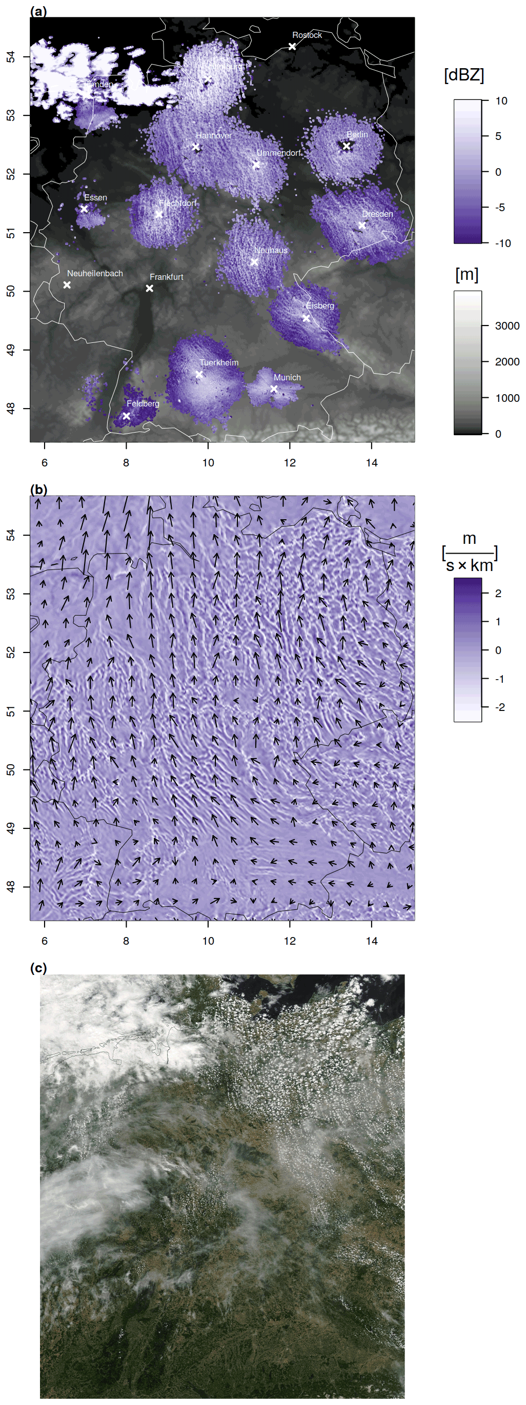
Figure 2 RADOLAN RX reflectivity in decibels relative to reflectivity (dBZ; blue) and orography in meters (grey shading) (a). COSMO-REA2 divergence (level 45 ≈200 m) (b) and Aqua MODIS satellite image (c) on 29 July 2009 at 12:00 UTC.

To get an idea of the type of data we rely on for our model validation, it is instructive to consider an example case. Figure 2a displays the RADOLAN RX image at noon on 20 July 2009. Aside from a few showers over the North Sea, no appreciable precipitation was observed in Germany on this warm summer day. Temperatures reached values in the high twenties and a high-pressure system centered near the German–Polish border generated weak southeasterly flow. Despite the absence of rain, most radars in the mosaic are surrounded by a disk of low but nonzero reflectivities (−10 to 5 dBZ). While the size, shape, and mean intensity of the disks vary, a consistent fine-scale cellular pattern can be observed throughout central, northern, and eastern Germany. Moreover, the regions of increased reflectivity are coherently organized in a line-like fashion along a SE–NW direction. Figure 2b, showing the corresponding wind and divergence field from COSMO-REA2, reveals that the orientation of the reflectivity lines is broadly consistent with the overall direction of low-level flow. Furthermore, the divergence field is characterized by small-scale patterns of cells and lines with alternating convergence and divergence, the size and orientation of which roughly resemble the radar pattern. Throughout eastern Germany, where the divergences are strongest, the satellite image in panel (c) shows the typical chains of cumulus clouds often associated with mesoscale shallow convection (Atkinson and Wu Zhang, 1996). A visual comparison of the reflectivities around, for example, the Berlin radar with the simulated divergences and the clouds in that region leads us to hypothesize that the boundary layer processes in COSMO-REA2 are not entirely unrealistic.

3.3 Data availability

As mentioned above, clear-air echoes typically only occur in a small environment around each radar. We therefore limit our study to circular regions with a 64 km radius, centered at the 16 radar stations that were active throughout the COSMO-REA2 period. With the exception of a few missing time steps due to technical errors, simulated divergences are readily available at every such grid point for each hour between 2007 and 2013. The availability of clear-sky echoes, on the other hand, depends on many factors including local topography, technical details of the radars, radar processing at the German weather service (DWD), and the life cycle of the biological scatterers. We consider an individual radar image incomplete if less than 50 % of pixels within our 64 km radius around the radar are above −10 dBZ (visual analysis of many example images has shown that no significant signals exist between roughly −10 dBZ and the smallest stored value of −32.5 dBZ). From the remaining data, we must filter out rainy episodes, defined here somewhat arbitrarily as cases in which at least 100 pixels exceed +10 dBZ. We will refer to all remaining images as complete.

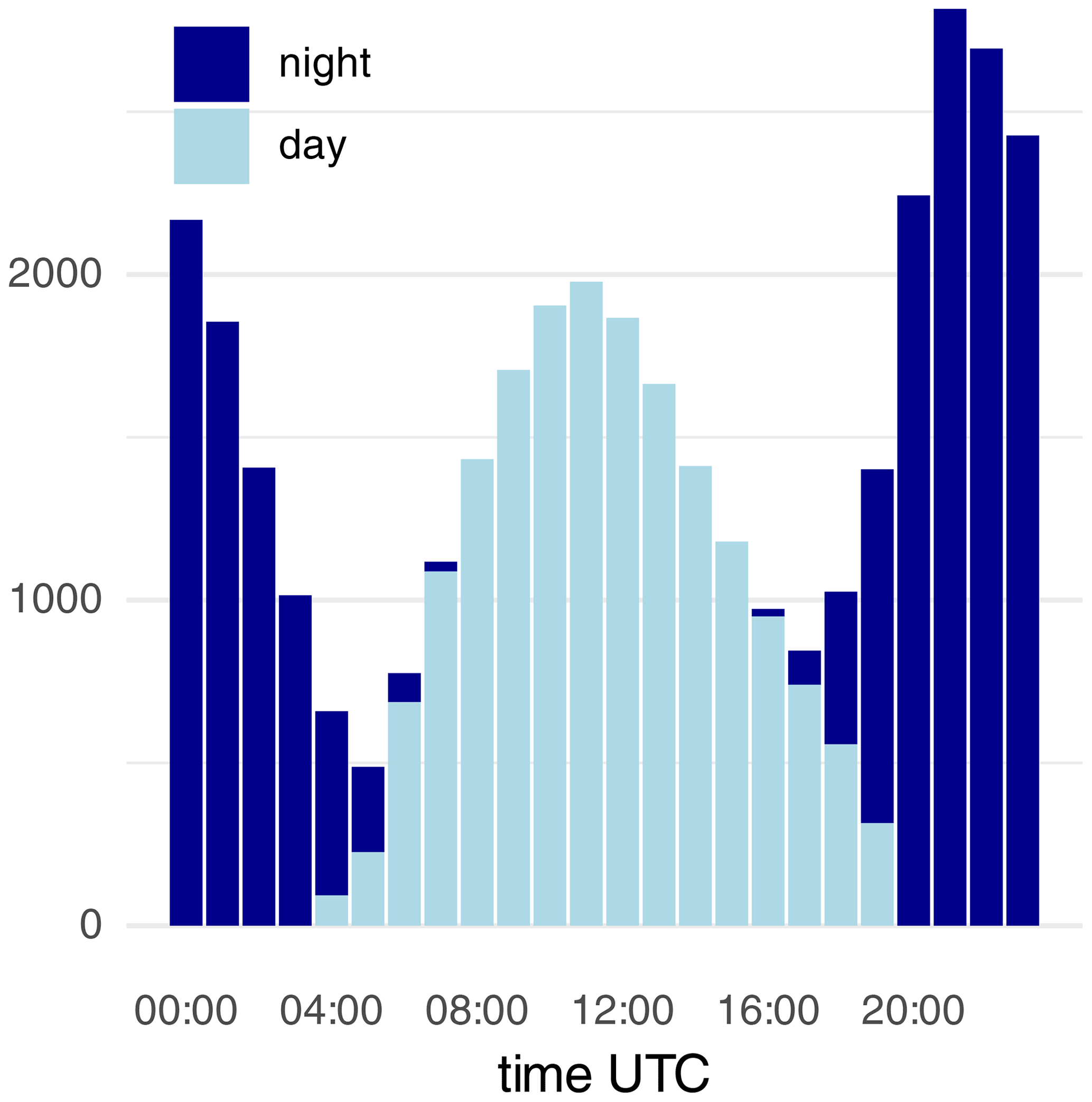
Figure 3 Number of complete clear-air radar echoes at the 12 selected radar stations, shown separately for night and day as defined by sunrise and sunset.

Table 1 Number of hourly incomplete, rainy, nighttime, and complete daytime hourly radar images per station. The top four radars are excluded from further analysis.

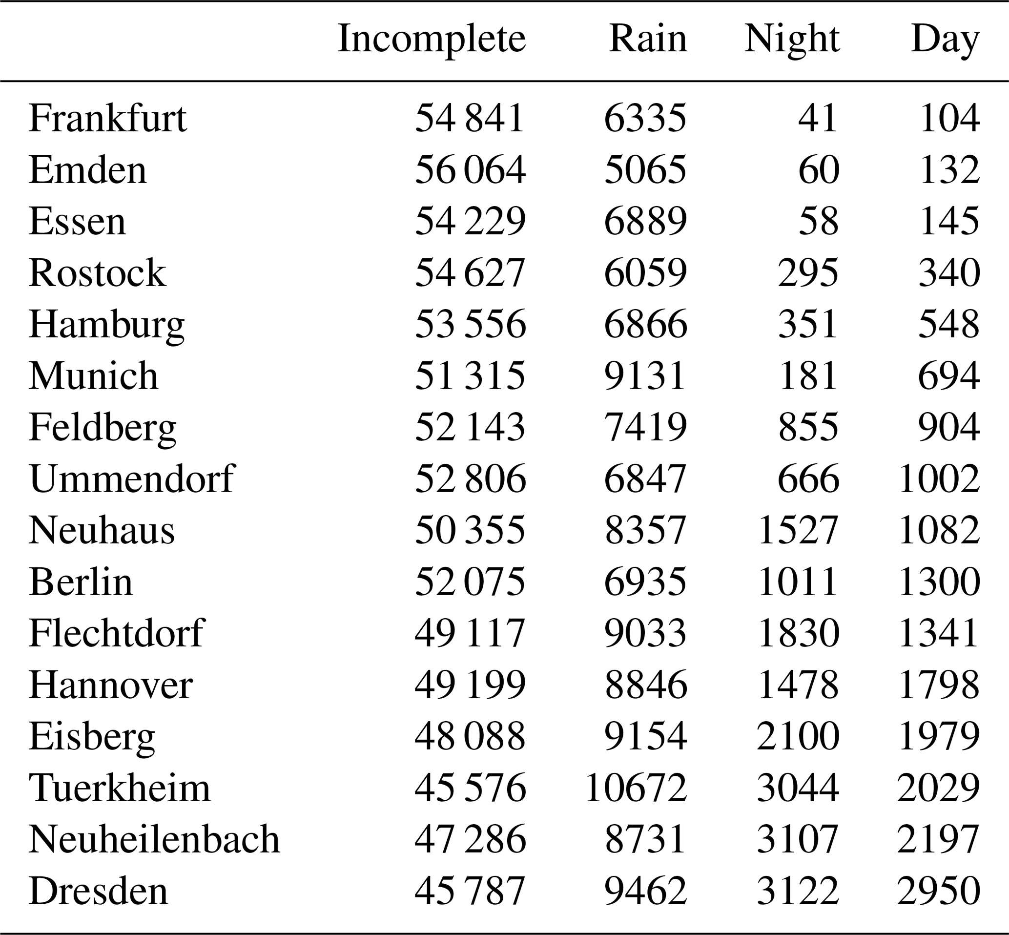
Table 2 Number of complete hourly non-rainy daytime radar echoes at the 12 selected radar stations.

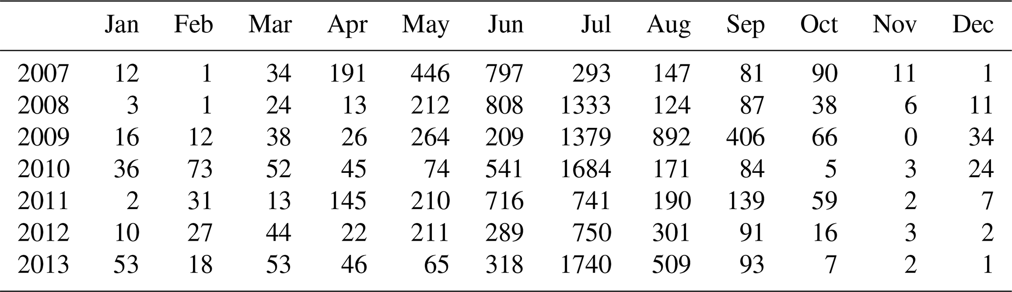
Table 1 shows that such complete clear-air echoes are overall rare (well below 5 % of all hourly images), and their frequency varies considerably between radars. For this study, we neglect the four radar stations with the fewest data, thereby removing two urban (Essen, Frankfurt) and two coastal locations (Emden, Rostock). The 12 remaining radars give us roughly 20 000 individual hourly images for comparison with COSMO-REA2. When studying the diurnal cycles below, we will furthermore include radar data at the full 5 min resolution, which gives us over 200 000 images.

In Table 2, we see that the vast majority of clear-sky echoes occur during summer, particularly June and July, with considerable variability between the years. The preference for the warm season is expected since both insect activity and boundary layer height are increased by higher temperatures. Consequently, the daytime frequency of available data follows a diurnal cycle as well (Fig. 3). In addition, there is a large second population of nighttime cases. The sudden increase in clear-air echoes at dusk, as well as their absence in winter, hints at migrating swarms of insects as a likely explanation (Drake and Reynolds, 2012). We exclude these data because (1) the weaker nighttime convergences are less likely to influence the pattern of the insect cloud, and (2) migrating swarms tend to inhabit thin layers near an atmospheric inversion, which only partly intersect the radar beam (see p. 237 f. in Drake and Reynolds, 2012).

4 Methods

4.1 Wavelet analysis

The idea of this study is to compare the correlation structures of the radar reflectivities and divergence fields summarized in terms of scale, anisotropy, and direction. To extract these properties from divergence and reflectivity images, we use the SAD methodology of Buschow and Friederichs (2021): the image to be analyzed is convolved with a series of localized 2D waveforms with varying scale and orientation. The analyzing filters are the so-called daughter wavelets, which are generated by shifting, scaling, and rotating a single carefully designed wave function, the mother wavelet. The square of one wavelet coefficient, i.e., the result convolving the image with one of the daughters, represents the amount of variance present at a particular location for a particular combination of spatial scale and orientation. The dual-tree complex wavelet transform (Selesnick et al., 2005) used in this study provides daughter wavelets with six orientations and up to J scales for an image of size 2^J×2^J. Following Buschow and Friederichs (2021), the three largest scales are removed because their support is larger than the image, rendering their interpretation ambiguous. After spatial averaging, a radar image with 128×128 pixels is thus summarized by 4×6 values, the so-called wavelet spectrum. To extract the scale, anisotropy, and direction from this spectrum, we treat the J×6 values as point masses arranged in a 3D space such that the six directions for one scale are at the vertices of a hexagon in the x−y plane, and the hexagons for the J scales are located at $z=\mathrm{1},\mathrm{\dots },J$. The center of mass of these point masses has three dimensionless components in cylindrical coordinates.

• The central scale $z\in [\mathrm{1},J]$ measures the dominant spatial scale of the image. If all variance is at spatial scale j, then z=j; if all scales contain equal variance, then $z=(J-\mathrm{1})/\mathrm{2}$.

• The radius $\mathit{\rho }\in [\mathrm{0},\mathrm{1}]$ describes the anisotropy. If all directions have equal variance, then the center of mass is in the middle of the hexagon and ρ=0; if all energy is concentrated in one direction, then ρ=1.

• From the angular coordinate, we can determine the dominant orientation angle $\mathit{\phi }\in [\mathrm{0}{}^{\circ },\mathrm{180}{}^{\circ }]$. Note that φ is only meaningful if the anisotropy ρ is nonzero.

For a detailed description of the calculation of these properties, as well as the details of the wavelet transform itself, we refer to Buschow and Friederichs (2021) and references therein. The software for this analysis is freely available in the open-source dualtrees R package (Buschow et al., 2020).

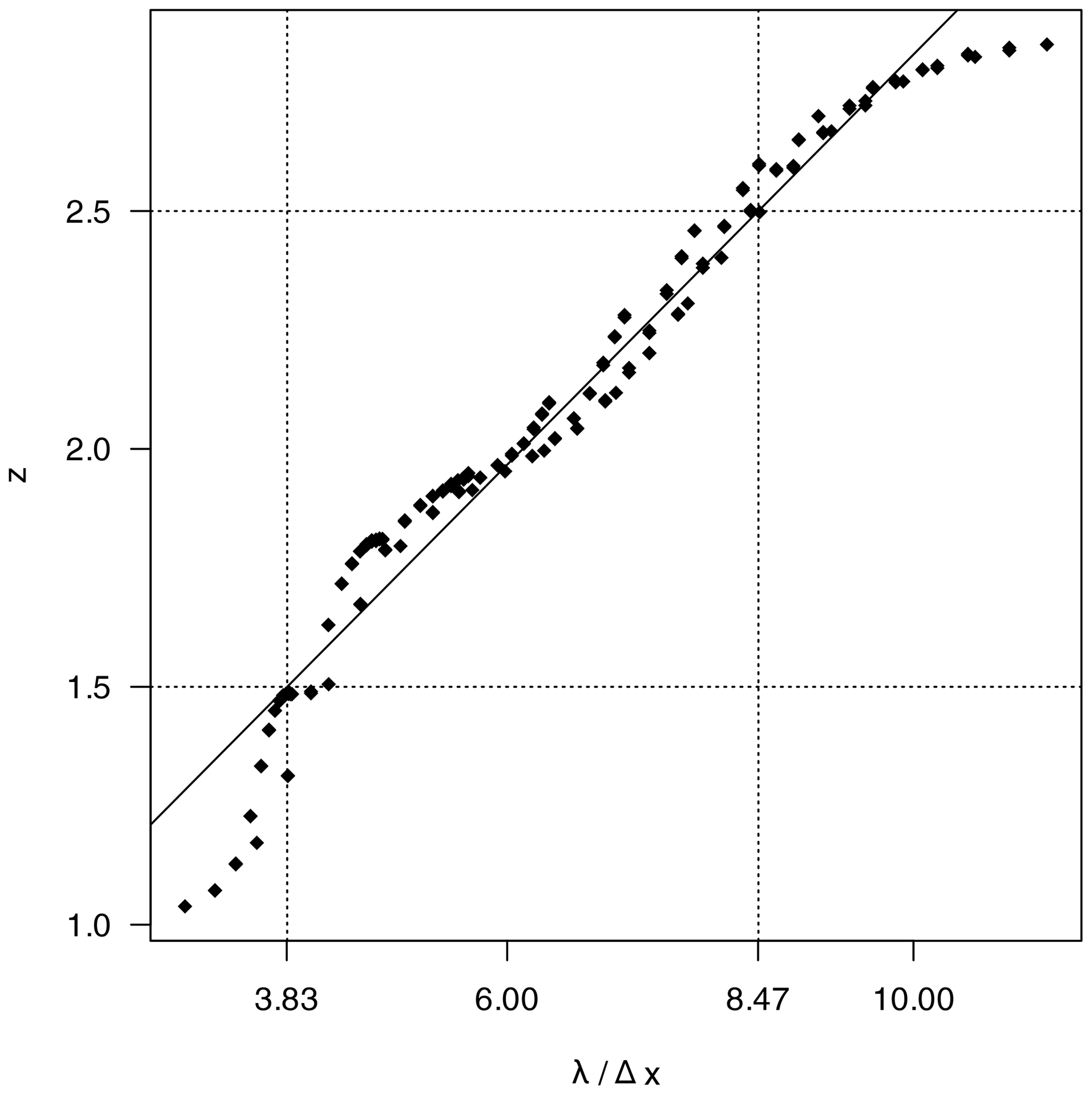
The central scale z is a dimensionless quantity, which cannot be analytically transformed into an equivalent Fourier wavelength. Since the actual physical size of the patterns is of some interest in the present study, we derive an empirical relationship based on test images with fixed wavelength in Appendix A. We find that, in the range of $\mathrm{1.5}<z<\mathrm{2.5}$, the relationship is well described by a linear fit with

$$\begin{array}{}\text{(2)}& {\displaystyle }\mathit{\lambda }\approx z\cdot \mathrm{9}\mathrm{km}-\mathrm{5.4}\mathrm{km}.\end{array}$$

It is important to note that this relationship is only approximately valid for the specific wavelets, scales, and wave-like test images used in the present study. This equivalent wavelength is furthermore not identical to the spacing between wave crests used as the measure of horizontal scale by Banghoff et al. (2020) because our λ includes also the scale perpendicular to the orientation of the features.

To make the distribution of angles φ interpretable, we compute the angles of intersection between φ and the model wind direction (averaged over the regions around each radar). A relative angle $\mathrm{\Delta }\mathit{\phi }=\mathrm{0}{}^{\circ }$ thus means that the patterns align with the wind direction, whereas $\mathrm{\Delta }\mathit{\phi }=\mathrm{90}{}^{\circ }$ indicates an orthogonal orientation.

4.2 Boundary conditions and pre-processing

The wavelet analysis described above requires data on a regular grid, ideally of size 2ⁿ×2ⁿ; to ensure fast computation times, discontinuities at the boundaries must be avoided. This is only a minor factor for intermittent fields like rain but very important for data with nonzero values along each border. To achieve periodic boundaries, we cut out a 128 km×128 km region (128 and 64 pixels for RADOLAN and COSMO-REA2, respectively) around each radar location and apply a circular Tukey window (Bloomfield, 2004) to smoothly reduce the field to zero (for divergences) or −10 dBz (for reflectivities) towards each side. A rectangular boundary would introduce spurious horizontal and vertical directions to the wavelet spectra.

For the reflectivity data, further pre-processing steps are required. Firstly, some radar images contain erroneous isolated pixels with unusual intensities that would artificially reduce the analyzed spatial scales. Following Lagrange et al. (2018), we therefore compare each pixel to the average over its eight nearest neighbors. If the difference is greater than 10 dBz, the pixel value is replaced by the neighborhood average. Secondly, the reflectivities around each radar often contain gaps of very small reflectivities ($<-\mathrm{10}$ dBz), caused for example by buildings, mountains, or water bodies without scattering insects. These arbitrarily shaped holes introduce an artificial pattern, which is unrelated to the wind field and needs to be removed. Here, we fill in the gaps with a simple algorithm that iteratively replaces values below −10 dBz with an average over the neighboring non-missing pixels. The details of the gap-filling algorithm, as well as a demonstration of its effectiveness, are given in Appendix B.

Lastly, a comparison between the wavelet spectra of two images would normally require that both datasets be given on the same grid. In our case, we can avoid re-gridding either field since the spatial resolutions differ by a factor of 2. The second scale in RADOLAN thus corresponds to the first scale of COSMO-REA2. We can therefore simply remove the smallest scale from the radar image to make the spectra comparable. We have checked that the results are virtually identical when the radar images are bilinearly re-mapped instead. The largest daughter wavelet that fits into our domain is j=4 for RADOLAN and j=3 for COSMO-REA2, giving us three comparable scales with six directions each.

5 Results

5.1 Climatology of divergence structures in COSMO-REA2

Based on Sect. 2, we can expect that small-scale, cellular circulations will form on warm sunny days, favored by high pressure and low wind speeds. Following the diurnal cycle of the boundary layer depth, these circulations start out small and become larger over the course of the day. According to Poll et al. (2017), Banghoff et al. (2020), and references therein, we furthermore expect to see a more linear mode of organization on windier days. The orientation of these roll-like structures will generally follow the mean wind direction (Weckwerth et al., 1997). Both cells and rolls should leave an imprint on the scale, anisotropy, and direction of the horizontal divergence fields. We therefore cut out square regions of 64×64 pixels around the 12 selected radar stations (Table 1) and apply the wavelet analysis described above for all hourly time steps from 2007 to 2013.

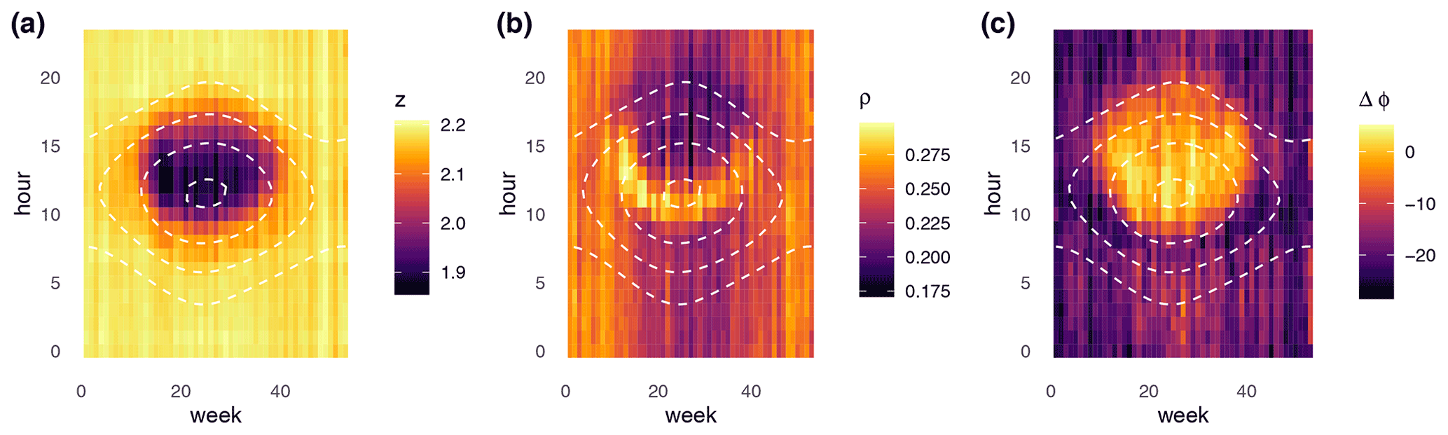
Figure 4 Average central scale (a), anisotropy (b), and angle relative to the mean wind (c),calculated from COSMO-REA2 (2007–2013) in the environment of the selected radar stations. White contours mark the sun's elevation angle at 0, 20, 40, and 60^∘.

As a first overview, we average the scale z, anisotropy ρ, and direction relative to the mean wind Δφ over the hours of the day and weeks of the year. Figure 4 shows that all three simulated variables undergo pronounced diurnal and annual cycles. During nighttime, the average central scales of the divergence fields remain close to z≈2 (about 13 km), with no strong variations between seasons. After the solar elevation exceeds roughly 40^∘, z approaches a clear minimum around noon before increasing again during the afternoon. Simultaneously, the anisotropy ρ reaches a maximum during the early hours of the small-scale phase before decreasing during the afternoon. Concerning the orientation of the divergence field (panel c), we observe that the small-scale pattern is typically aligned with the mean wind direction, while the larger-scale nighttime and winter patterns are not.

As expected, the simulated small-scale circulations thus impress their diurnal life cycle on the mean spatial structure of the divergence field. To see how prominent these features are compared to the overall variability, we now consider probability densities of the three structural quantities separated by season and time of day (Fig. 5).

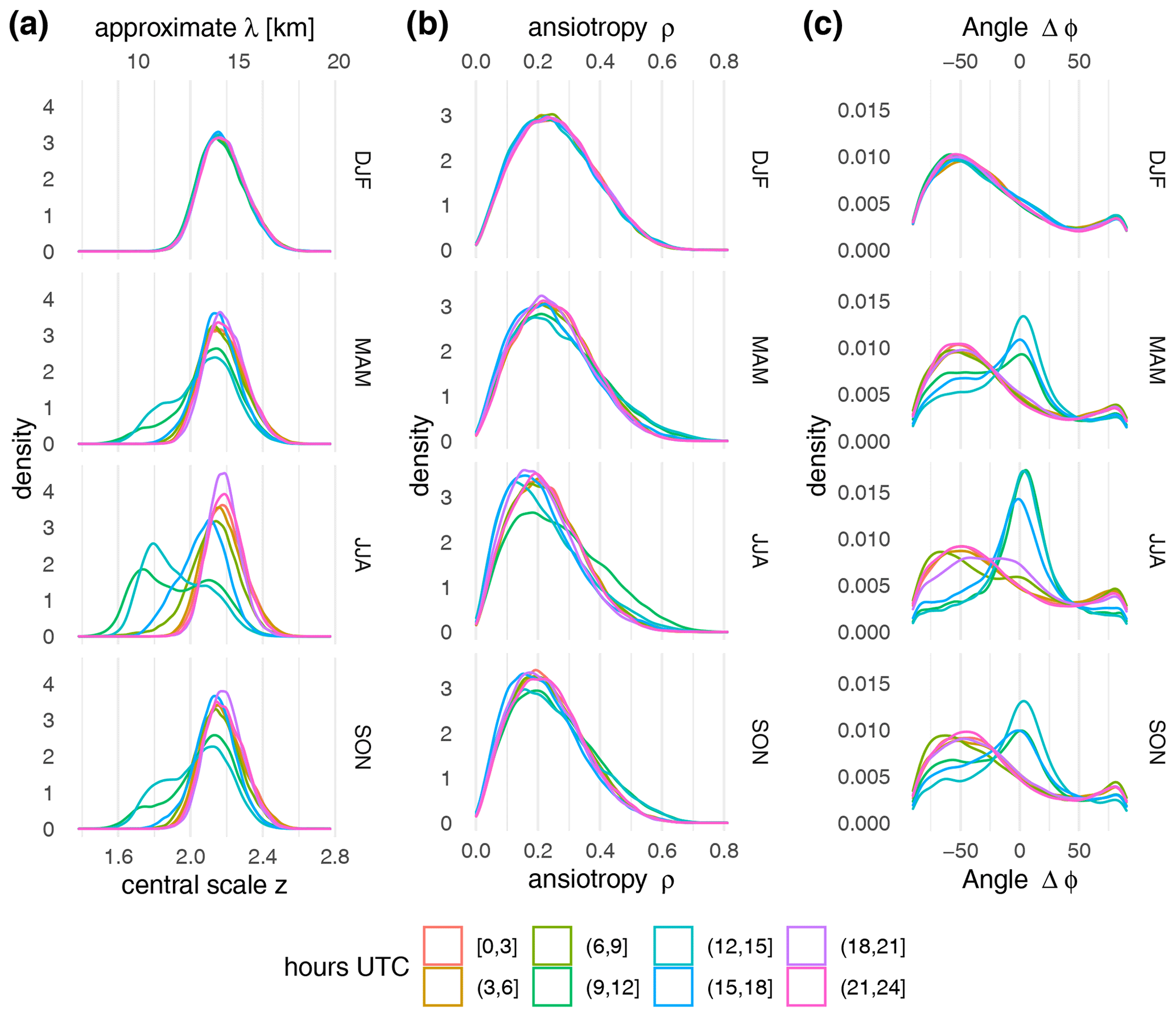
Figure 5 Estimated probability densities (kernel estimates) for the scale z (a, converted into an approximate wavelength λ via Eq. 2), anisotropy ρ (b), and relative angle Δφ (c) for different seasons (from top to bottom winter, spring, summer, and autumn) and times of day.

For the spatial scales in panel (a), we find that the prominent minimum around noon is indeed a common occurrence in all seasons except winter, indicated by bimodal distributions between 09:00 and 15:00 UTC. During summer in particular, the smaller-scale mode, centered near z≈1.75 or λ≈10 km, is more likely than z>2. The two modes can be seen with similar clarity in the distribution of orientations (Fig. 5c): during winter or nighttime, orientations along the wind direction are rare, and most angles are closer to $-\mathrm{75}{}^{\circ }$. In the other three seasons, Δφ≈0 is by far the most likely value during daytime. The signal in the anisotropy (Fig. 5b), on the other hand, is far weaker: a clearly increased likelihood for anisotropic features is only evident in summer between 09:00 and 12:00 UTC, and the change in the distribution is far less pronounced than for z. While the formation of exceptionally small structures, oriented along the mean wind, is thus a common occurrence, the increased linearity around noon seen in Fig. 4b can only occasionally be observed.

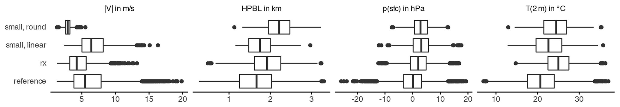
Figure 6 COSMO-REA2 level-45 wind speed, boundary layer height, surface pressure anomaly, and 2 m temperature during summer (JJA) between 11:00 and 13:00 UTC, averaged around the selected radar locations. “Small and round” cases have $z<\mathrm{1.68},\mathit{\rho }<\mathrm{0.08}$, and “small and linear” cases have $z<\mathrm{1.68},\mathit{\rho }>\mathrm{0.46}$. The values for all remaining cases are included in the “reference” box plots. The box plot labeled “rx” contains all instances in which at least one clear-air radar echo is available.

Next, we are interested in the typical weather situation associated with the occurrence of these small and/or linear patterns. To this end, we focus on the 3 h around noon during the summer season and search for cases in which both ρ and z are in the bottom 10 % of their climatological distribution (“small and round” mode). For the “small and linear” mode, we select those cases in which z is in the bottom 10 %, whereas ρ is in the top 10 % of its distribution. At time steps that meet either of these two criteria, as well as the remaining “reference” cases, we compute spatial averages around the selected radar stations for several relevant variables from COSMO-REA2.

Figure 6 shows that boundary layer height, 2 m temperature, and surface pressure undergo a moderate increase during time steps with small and linear patterns and a stronger increase if the pattern is small and round. In the latter cases, the median temperature is close to 25 ^∘C and the boundary layer rarely falls below 2 km. Simultaneously, the average wind speed is strongly reduced. Conversely, the small and linear mode is associated with a slightly increased wind speed. Hence, the boundary layer circulation in COSMO-REA2 qualitatively resembles Rayleigh–Bénard convection.

In preparation for the quantitative comparison with radar data, Fig. 6 also includes the environmental conditions for days on which at least one clear-sky RADOLAN image is available (box plots labeled “rx”). We find that the radar echoes occur mostly on very warm days with moderately increased boundary layer depth and decreased wind speeds. This is consistent with the assumption of insects as the primary origin of these echoes. The observations thus mostly sample cases in which small-scale circulations are likely to occur.

5.2 Verification against radar reflectivities

In this section, we attempt to partly assess the realism of our model-based climatology using the clear-sky radar reflectivity data from RADOLAN. Besides cases with too many missing or rainy pixels, we also exclude all nighttime images. The remaining data are subjected to the wavelet analysis as described in Sect. 4.2.

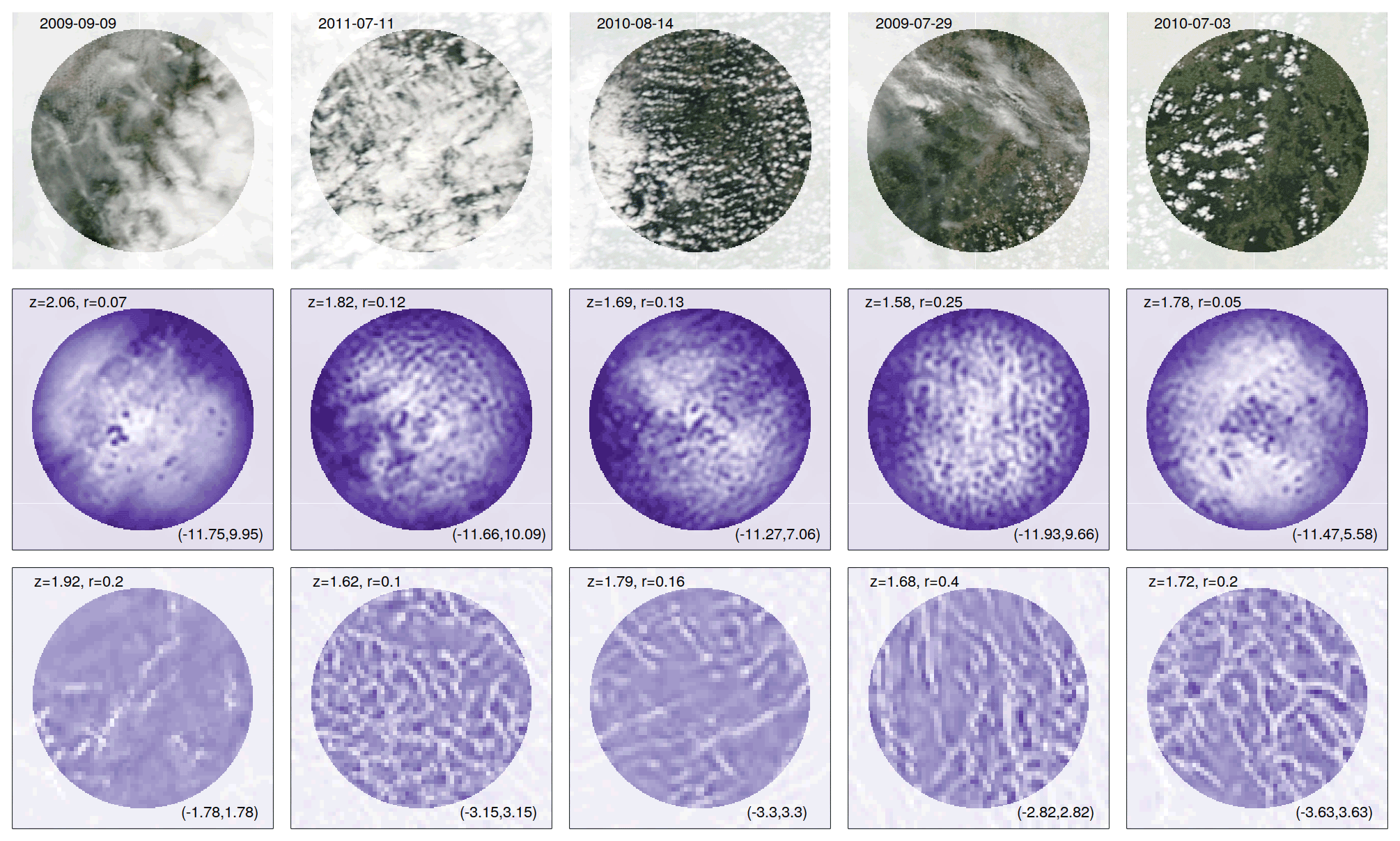
Figure 7 Randomly selected examples from the set of available non-rainy 12:00 UTC radar images at Flechtdorf. Top row: Aqua MODIS snapshots (http://wvs.earthdata.nasa.gov, last access: 2 November 2021, timing only approximately matches 12:00 UTC). Middle: RADOLAN RX reflectivity. Bottom: COSMO-REA2 level-45 divergence. Light colors indicate high reflectivity and convergence, respectively. Numbers in the top left corner indicate the analyzed scale and anisotropy; the range of reflectivity and divergence values is given in the bottom right.

Before analyzing the statistics of the entire dataset, we briefly consider a few individual examples. Figure 7 shows five randomly selected cases from the Flechtdorf radar station. The 12:00 UTC time step was chosen so that a visible satellite image from MODIS is available at approximately the same time. For consistency with the wavelet-based analysis, we have removed the smallest-scale features from the RADOLAN images by transforming to wavelet space, setting the coefficients at level 1 to zero, and transforming back.

Due to the naturally noisier character of the radar images, the immediate visual similarity between the radar and model is not great. Upon closer inspection, we nonetheless recognize some common features: on 9 September 2009 neither the radar nor model show any organized structures under the closed cloud cover. The other four cases each feature organized small-scale patterns with somewhat similar values of z<1.9 in both datasets. 29 July 2009 (second from the right and incidentally also our example from Fig. 2) is recognized as the most linear pattern by ρ≥0.2, although the zoomed-in view makes it somewhat harder to discern this visually in the radar image (compare Fig. 2 where this is more obvious).

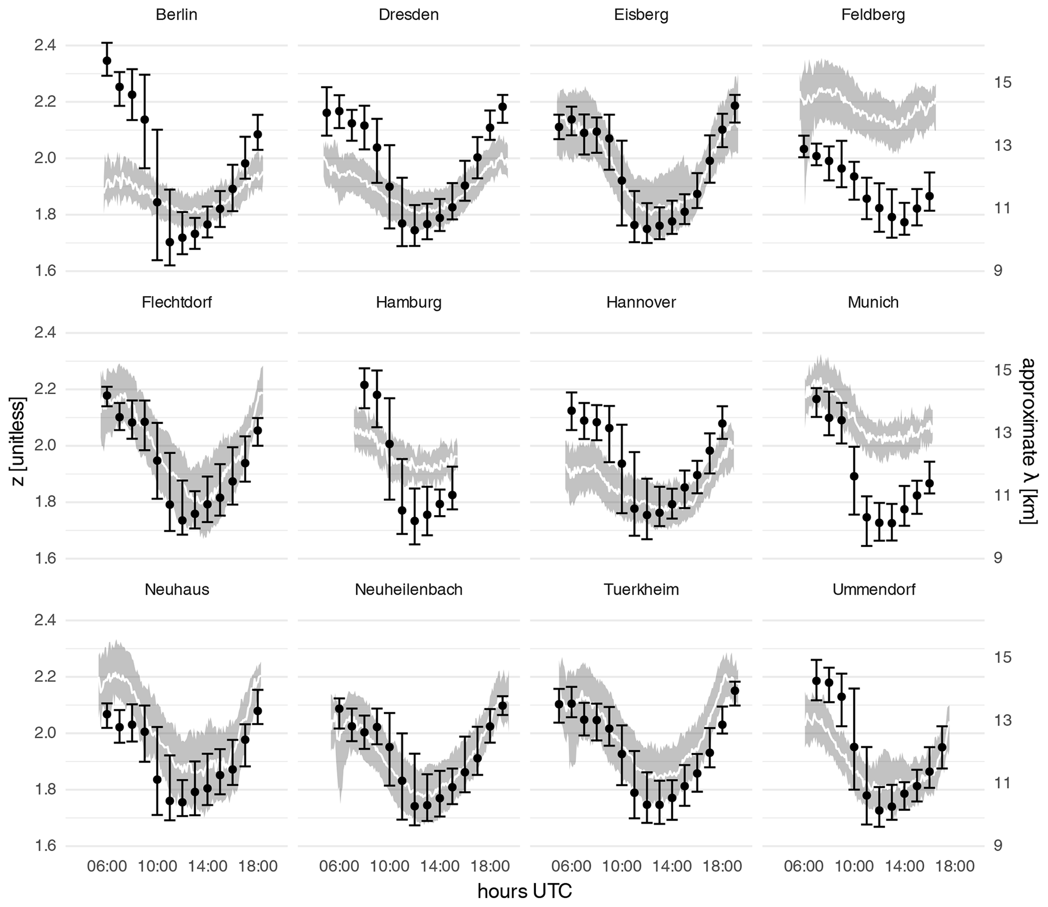
Figure 8 Diurnal cycles of spatial scales from 5 min radar data (areas and lines) and hourly COSMO-REA2 10 m divergence (points and error bars). The grey area and error bars indicate the interquartile range, and the white line and black dots mark the median. Only cases with complete (see Sect. 3.3) clear-air echoes are included.

Figure 8 shows a quantitative comparison of the modeled and observed diurnal cycles of central scales. In addition to the hourly data for which corresponding COSMO-REA2 divergences are available, we have included all other 5 min time steps with complete clear-air echoes as well. The results can be separated into two main groups: at the rural radar stations in Eisberg, Flechtdorf, Neuhaus, Neuheilenbach, Turkheim, and Ummendorf, the agreement between the model and observations is surprisingly good. COSMO-REA2 reproduces not only the correct evolution of the diurnal cycle but also similar spatial scales with a large overlap in the interquartile ranges. In contrast, the observed spatial patterns at the three largest German cities of Berlin, Hamburg, and Munich differ significantly from the modeled values, as well as from the other stations. Hannover and Dresden have more data than the other urban locations (see Table 1) and show better agreement with the model. Here, the observed cycle is flatter but resembles its modeled counterpart in the afternoon. The unusual behavior of the Feldberg station is likely the result of its mountainous surroundings, which cause both additional ground clutter and changes to the local circulation, neither of which is resolved by the 2 km model orography. It is worth noting, however, that despite the offset, both datasets agree that the smallest-scale patterns occur later in the day than at other stations. This effect may be related to the generally lower surface temperatures (and thus Rayleigh numbers) at higher altitudes.

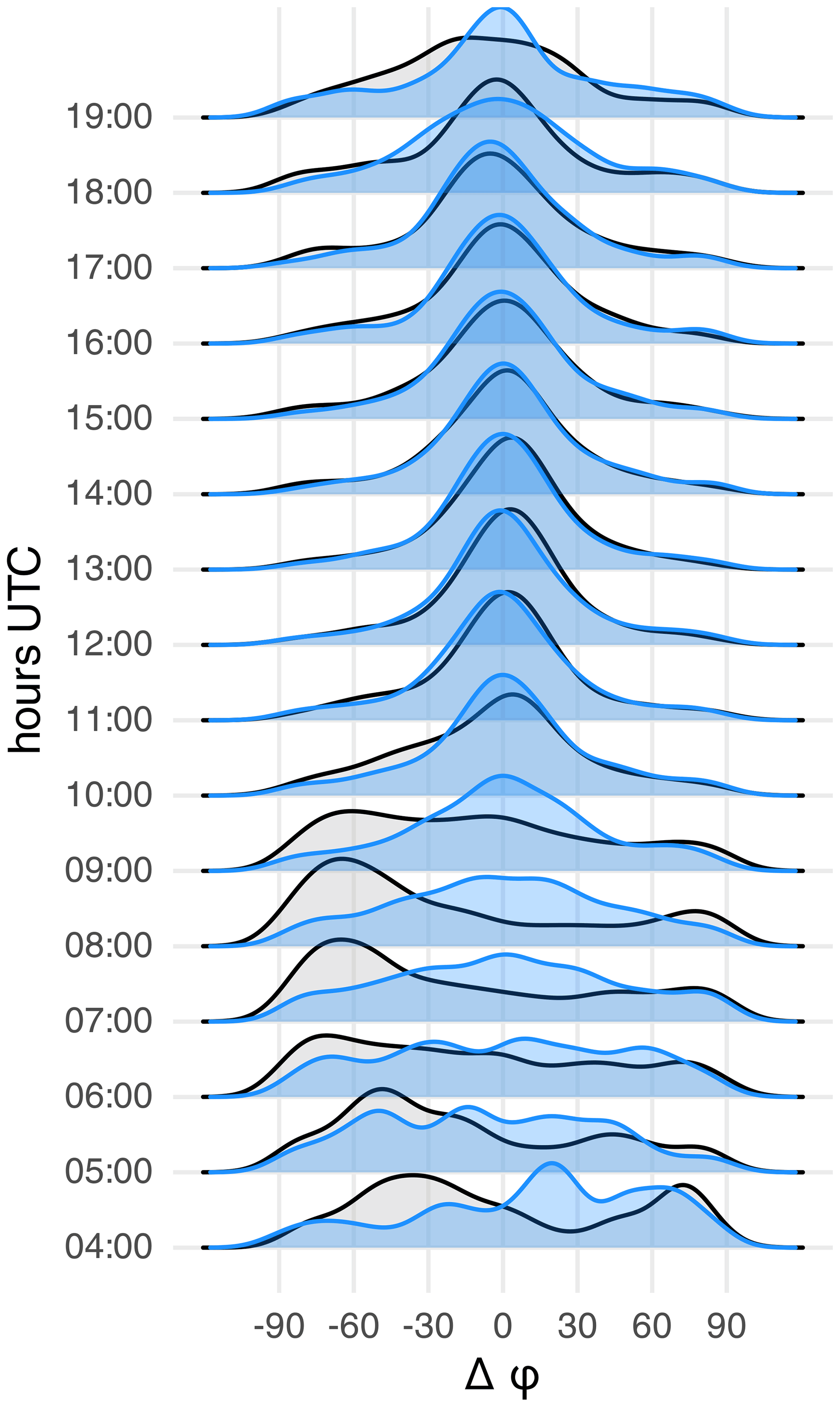
Figure 9 Distribution of orientations relative to the COSMO-REA2 mean wind throughout the day. COSMO-REA2 is shown in black, and RADOLAN is shown in blue. Only complete, non-rainy daytime cases with ρ(RADOLAN)>0.1 are included.

Good agreement between the model and observations can be seen in the distribution of the angle φ as well. In Fig. 9, we have pooled all radars together and consider only full hours during which the model wind direction is known. Cases with small observed anisotropy (ρ≤0.1), i.e., ambiguous orientation, were removed as well. We find that, between 10:00 and 17:00 UTC, both sets of images are usually oriented within $\pm \mathrm{15}{}^{\circ }$ of the mean model wind direction; the distributions of RADOLAN and COSMO-REA2 match almost perfectly. Before and after this interval, which coincides with the small-scale phase of the diurnal cycle, a wider variety of orientations is possible.

Figure 10 As Fig. 8, but for ρ and without separation by radars.

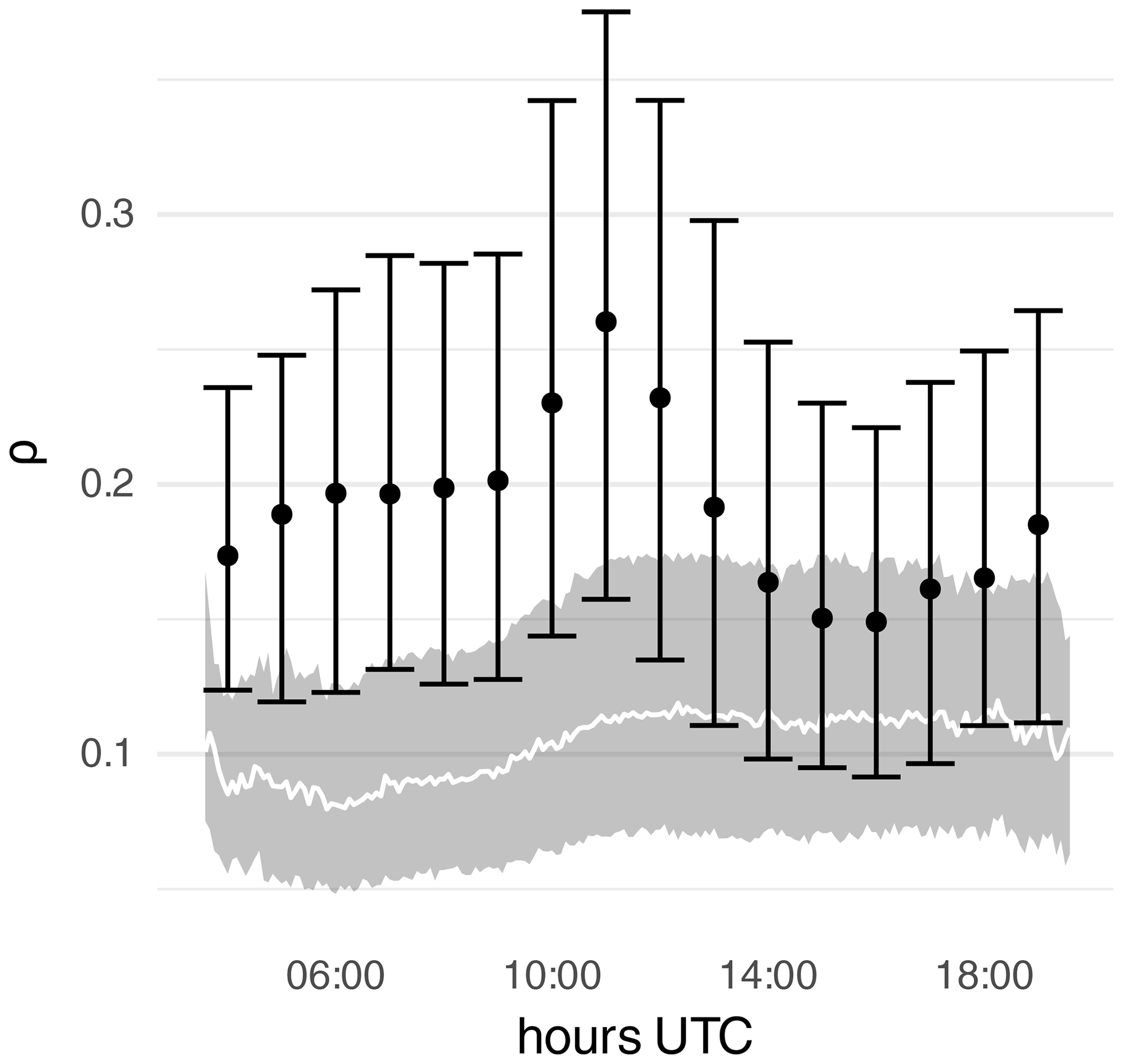
While the scale and orientation are thus in reasonably good agreement, the same cannot be said for the anisotropy. Figure 10 shows that the observations are almost universally more isotropic than the model fields. The pattern of increasing linearity towards a maximum before noon seen in Fig. 4b is clearly present in this sample of the model data. The observations, on the other hand, hardly contain this pattern at all, with only a very weak maximum at 11:00 UTC and nearly constant values during the afternoon.

Aside from the climatological distribution and diurnal cycle, we are interested in the model's ability to represent the day-to-day variability of the spatial divergence patterns. For z and ρ, we can eliminate the overall bias and diurnal behavior by subtracting the long-time mean for every daytime hour from the respective time series. To avoid residual effects of the annual cycle, we limit this analysis to the summer season. Timing errors within each day are furthermore removed by taking the daily minimum of z and maximum of ρ. Figure 11a reveals that the remaining scale anomalies in COSMO-REA2 and RADOLAN are slightly correlated with many remaining errors below 0.1 and almost all below 0.2 (outer lines). As expected, the correlation is even lower for ρ (Fig. 11b), and the typical errors are relatively large even after the bias has been removed.

6 Discussion

The results of Sect. 5.1 and 5.2 raise several intertwined questions: what level of realism can be expected of the reanalyzed small-scale structure? To what extent can the RADOLAN dataset be used to validate the simulation? How appropriate was the wavelet-based analysis for the task at hand? Concerning the trustworthiness of COSMO-REA2, it must be remembered that the local divergence patterns are primarily the product of the model dynamics and parameterized turbulence, not the data assimilation. The environmental conditions that drive the formation of a particular mode of small-scale organization, however, can be expected to have good accuracy due to the continuous input of wind speed, humidity, and pressure from weather stations. It is therefore not surprising that the model can accurately represent diurnal and annual cycles and differentiate between days with organized and unorganized situations. Consequently, the model climatology as described in Sect. 5.1 qualitatively agrees with our expectations from the literature. Whether or not the simulated small-scale structure itself can be trusted is questionable in light of the theory discussed in Sect. 2. Our comparison with RADOLAN clear-air data suggests that, despite the proximity to the grey zone, the modeled structures are not overall unrealistic. In interpreting this result, we must recall that the difference in native resolution between RADOLAN and COSMO-REA2 was handled by deleting the smallest scale from RADOLAN. We have thereby filtered out any variability below the model's effective resolution. Figure 8 therefore does not indicate that the mesoscale model successfully simulates the spatial scales present in the real atmosphere. We can merely see that the remaining variability (upwards of λ≈8 km), which both datasets can represent, matches the observed diurnal cycle decently, especially at the rural stations.

As predicted by Zhou et al. (2014), the wavelengths of the simulated eddies are near the smallest scale resolved by the model. We note, however, that the underlying resolution of RADOLAN is 1^∘ in azimuth and 250 m in range direction. Inside our 64 km radius, and particularly close to the radar, the internal resolution of the measurements is considerably finer than the 1 km×1 km grid used . There is thus no obvious technical reason why, after filtering, RADOLAN should have to exhibit increased variability on the same scale as the model. We have experimentally recalculated the central scales of the radar images including the previously removed smallest scales and found a slight shift in the cycle towards earlier hours. Conversely, if we remove the second-smallest scale as well, a shift in the opposite direction emerges. This supports our interpretation that the model simulates the patterns seen in the observations with an approximately correct diurnal cycle on the scales we included; smaller-scale variability, which would initiate earlier in the day, is resolved by neither COSMO nor RADOLAN. The filtering to common scales also explains the nonintuitive fact that radar structures appear to be slightly larger than those of the model in Fig. 8. It should furthermore be noted that we make no direct statements about the intensity (variance) of the circulations. Such information cannot easily be inferred because the absolute radar reflectivities depend on the technical details of the radar, applied pre-processing, and the unknown overall concentration of biological scatterers.

The greater disagreement at the urban radar locations has two main explanations. On the one hand, it is likely that buildings and unrelated radio signals introduce excessive noise into the images, overshadowing the natural signal. This explanation is supported by the lack of complete images at the Essen and Frankfurt stations, both of which are located in highly urbanized regions (Frankfurt is the city with the most skyscrapers in Germany). On the other hand, the urban landscape itself can influence the near-surface circulation in ways that are not resolved by the model. The similar effects of small-scale orography likely explain the special behavior at the Feldberg station.

Aside from spatial scales, the anisotropy of the divergence pattern, i.e., the difference between linear and cellular organization, is of interest. Here, the model's tendency towards more linear patterns earlier in the day could not be confirmed observationally. On the one hand, it is plausible that the lack of finer-scale variability leads to the simulation of unnaturally regular stripes. On the other hand, gaps and noise have a larger impact on the anisotropy than the scale (see Appendix B), making these results somewhat less robust.

Lastly, it should again be emphasized that our clear-air dataset provides no information on nighttime and winter and is biased towards cases with high temperatures at which small-scale circulations are likely to occur. Our validation is therefore mostly conditional on the occurrence of these phenomena; whether or not the model correctly differentiates between days with and without organized shallow convection could only partly be judged (see Fig. 11).

7 Conclusions and outlook

The main goal of this study was to explore the use of clear-sky radar data for the evaluation of simulated low-level divergence structures. A wavelet-based verification methodology, developed and extensively tested for precipitation data, was used to summarize the spatial patterns in terms of scale, anisotropy, and direction. We have demonstrated that model-based divergences and radar reflectivities are comparable at this level of abstraction. Our investigation of the German radar network has shown that usable clear-sky echoes are rare overall and almost nonexistent in winter. This supports the assumption that such daytime echoes are caused by small insects, the life cycle and habitats of which may also explain the substantial differences between radars as well as strong year-to-year variations. The relatively long time span from 2007 to 2013 nonetheless resulted in a robust dataset of over 20 000 individual images, mostly during summer, for which the modeled patterns could be verified against spatial observations. At most radar locations, both datasets show a very similar diurnal cycle in the spatial scales and orientations, with a strong preference for small-scale (λ≈10 km) features around noon. The orientation during the small-scale phase of the cycle is almost always within 15^∘ of the mean wind. The fact that this observation holds for both datasets also implicitly confirms that the model adequately represents the mean wind direction. COSMO-REA2 furthermore simulated a trend towards increasingly linear features at the start of the small-scale phase, which could not be found in the observations. As discussed above, a more complete set of observations might be able to clarify whether this indicates deficiencies of the model, the observations, or (likely) both.

Based on the overall decent agreement with the radar observations, we may put some limited trust in the model's behavior in the unobserved parts of the time series as well. If COSMO-REA2 is thus to be believed, mesoscale shallow convection, favored by high pressure (clear skies) and temperatures, as well as weak winds, is a common occurrence in Germany in all seasons except winter; during JJA, the small-scale mode is more likely than the larger-scale configuration. Its onset a few hours after sunrise is characterized by a transition phase with larger-scale, isotropic divergence patterns, the orientation of which switches from ∼70 to $\sim \mathrm{0}{}^{\circ }$ with respect to the mean wind direction. While most patterns are isotropic, i.e., cellular in nature, there is also a weaker signal of linear organization. This more roll-like mode is most often simulated during JJA between 09:00 and 12:00 UTC and preferably occurs when winds are unusually strong and the boundary layer is shallower than in the cellular cases. These simulated features are qualitatively consistent with the theory, as well as previous observations of mesoscale shallow convection.

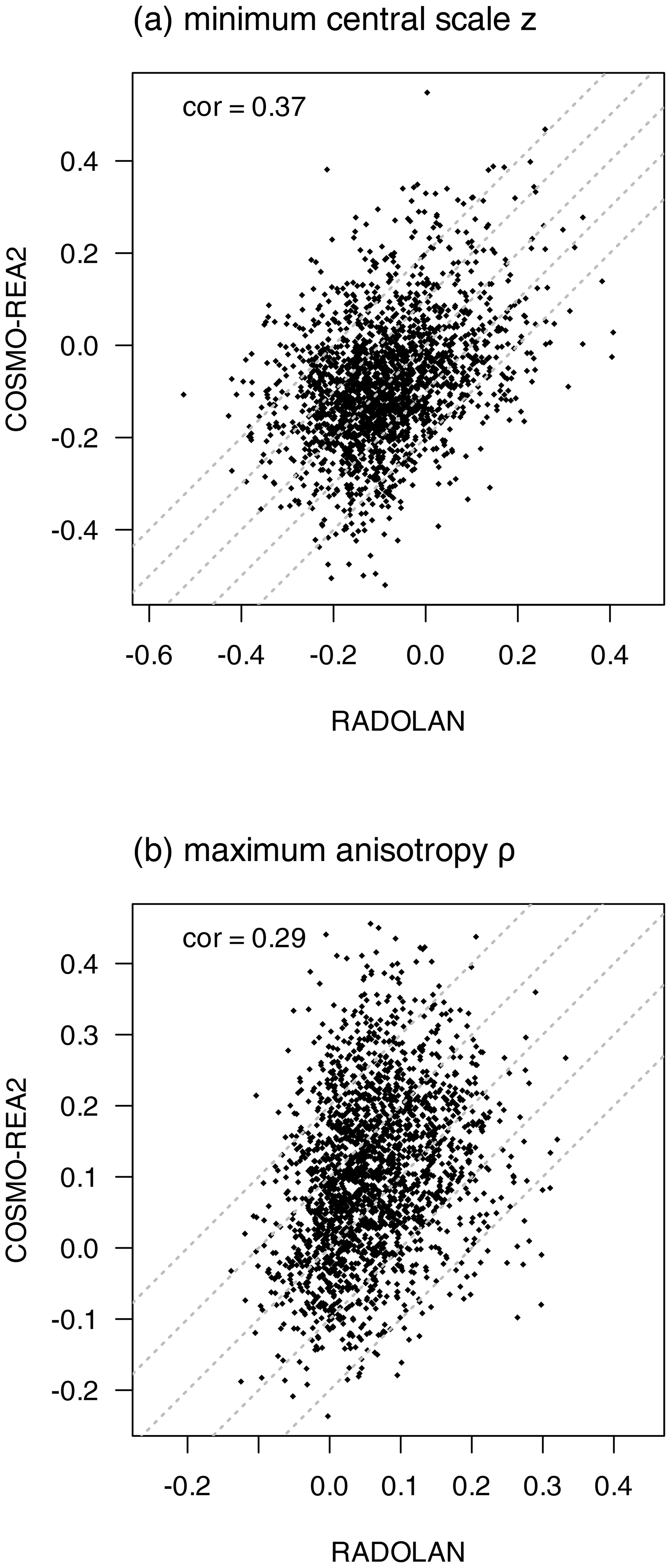
Figure 11 Scatterplot of daytime minimum scale (a) and daytime maximum anisotropy (b) anomalies during daytime in summer (JJA) from RADOLAN (x axis) and COSMO-REA2 (y axis). Anomalies were calculated by subtracting the respective mean values from every hour of the day. Dashed lines mark errors d$z,\mathrm{d}\mathit{\rho }=\mathit{\{}-\mathrm{0.2},-\mathrm{0.1},\mathrm{0},\mathrm{0.1},\mathrm{0.2}\mathit{\}}$.

Concerning future prospects, it must be emphasized that we have relied on only the most widely available kind of radar observations. Modern dual-polarization Doppler radars produce a wealth of further information, which would, for example, allow us to confidently separate insect-related echoes from unhelpful noise and clear up the nature of the nighttime echoes (Zrnic and Ryzhkov, 1998; Melnikov et al., 2015). Additionally, parameters like mean wind speed and direction, and even the boundary layer height (Banghoff et al., 2018), could be inferred directly from the radar instead of relying on the model (Banghoff et al., 2020). Lastly, we re-iterate that small scales below ∼8 km were filtered out in this study in order to fairly evaluate the mesoscale model. Depending on their frequency, weather radars can observe much finer details of the turbulent boundary layer. A strategy similar to ours could therefore also provide useful information for the objective validation of realistic large-eddy simulations as in Thurston et al. (2016), Poll et al. (2017), Bauer et al. (2020), Ito et al. (2020), and Pantillon et al. (2020).

Appendix A: Empirical relationship between scale and wavelength

Figure A1 Wavelength $\mathit{\lambda }=\mathrm{1}/\sqrt{k_x^{\mathrm{2}}+k_y^{\mathrm{2}}}$ against central scale z.

To approximately translate the central scale into an equivalent Fourier wavelength λ, we apply the exact method described in Sect. 4.2 to synthetic test images of pure sine waves given by

$${\displaystyle }f(x,y)=\sin \left(\mathrm{2}\mathit{\pi }(k_{x}x+k_{y}y)\right)+\mathit{ϵ},$$

where ϵ is a Gaussian white noise term with zero mean and variance 0.04. Figure A1 shows that the relationship between z and λ is nearly linear for this idealized signal. For z<1.5 and z>2.5, the curve becomes nonlinear because most variance is outside the range of scales covered by our wavelet transform. The linear fit yields $\mathit{\lambda }/{\mathrm{\Delta }}_x=\mathrm{4.464}\cdot z-\mathrm{2.765}$. Since we are merely interested in a rough approximation with round numbers, we simplify the result for Δ_x≈2 km to obtain Eq. (2).

Appendix B: Filling the gaps in the radar images

For this study, we are not interested in the radar reflectivities themselves or even their full spatial correlation function, but only the estimates' structural characteristics $\mathit{\rho },\mathit{\phi },z$. To mitigate the effects of holes, i.e., regions with $Z\le -\mathrm{10}$dBZ, in the radar images, we implement a simple iterative algorithm to smoothly fill in the gaps: (1) find missing points with at least one non-missing neighbor, (2) replace values of those points with an average over the up to eight adjacent non-missing values, and (3) repeat from (1) until all gaps are filled. The result is similar to inverse distance interpolation but (at least in our implementations of the two algorithms) considerably faster.

To test the success of our approach, we select 300 nearly complete (less than 3 % missing data) clear-air radar echoes from our dataset and artificially add the gaps from 300 other randomly selected incomplete images. In Fig. B1, we compare ρ,φ, and z estimated with and without the gap-filling algorithm. As expected, the impact of the gaps is massive, but our algorithm mostly mitigates the effects. We have repeated the experiment with inverse distance interpolation (not shown) and found no substantial improvement over the iterative procedure.

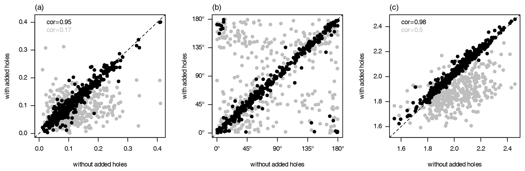
Figure B1 Anisotropy ρ (a), angle φ (b), and scale z (c) estimated from nearly complete images (x axis) and images with added holes (y axis). Black dots show the results of the iterative gap-filling algorithms; values obtained without gap filling are shown in grey. Correlations between the x and y values are shown in the top left corner for both estimates in the corresponding color. Linear correlations are not helpful for the circular quantity in panel (b) and were thus omitted.