The interpretation of temperature and salinity variables in numerical ocean model output and the calculation of heat fluxes and heat content

The international Thermodynamic Equation of Seawater 2010 (TEOS-10) defined the enthalpy and entropy of seawater, thus enabling the global ocean heat content to be calculated as the volume integral of the product of in situ density, ρ, and potential enthalpy, h⁰ (with reference sea pressure of 0 dbar). In terms of Conservative Temperature, Θ, ocean heat content is the volume integral of $\mathit{\rho }{c}_p^{\mathrm{0}}\mathrm{\Theta }$, where $c_p^{\mathrm{0}}$ is a constant “isobaric heat capacity”.

However, many ocean models in the Coupled Model Intercomparison Project Phase 6 (CMIP6) as well as all models that contributed to earlier phases, such as CMIP5, CMIP3, CMIP2, and CMIP1, used EOS-80 (Equation of State – 1980) rather than the updated TEOS-10, so the question arises of how the salinity and temperature variables in these models should be physically interpreted, with a particular focus on comparison to TEOS-10-compliant observations. In this article we address how heat content, surface heat fluxes, and the meridional heat transport are best calculated using output from these models and how these quantities should be compared with those calculated from corresponding observations. We conclude that even though a model uses the EOS-80, which expects potential temperature as its input temperature, the most appropriate interpretation of the model's temperature variable is actually Conservative Temperature. This perhaps unexpected interpretation is needed to ensure that the air–sea heat flux that leaves and arrives in atmosphere and sea ice models is the same as that which arrives in and leaves the ocean model.

We also show that the salinity variable carried by present TEOS-10-based models is Preformed Salinity, while the salinity variable of EOS-80-based models is also proportional to Preformed Salinity. These interpretations of the salinity and temperature variables in ocean models are an update on the comprehensive Griffies et al. (2016) paper that discusses the interpretation of many aspects of coupled Earth system models.

1 Introduction

Numerical ocean models simulate the ocean by calculating the acceleration of fluid parcels in response to various forces, some of which are related to spatially varying density fields that affect pressure, as well as solving transport equations for the two tracers on which density depends, namely temperature (the CMIP6 variables identified as thetao or bigthetao) and dissolved matter (“salinity”, CMIP6 variable so). For computational reasons it is useful for the numerical schemes involved to be conservative, meaning that the amount of heat and salt in the ocean changes only due to the area-integrated fluxes of heat and salt that cross the ocean's boundaries; in the case of salt, this is zero. This conservative property is guaranteed for ocean models to within computational truncation error since these numerical models are designed using finite-volume integrated tracer conservation (e.g. see Appendix F in Griffies et al., 2016). It is only by ensuring such conservation properties that scientists can reliably make use of numerical ocean models for the long (centuries and longer) simulations required for climate and Earth system studies.

However, this apparent numerical success ignores some difficult theoretical issues with the equation set being numerically solved. Here, we are concerned with issues related to the properties of seawater that have only recently been widely recognized because of research resulting in the Thermodynamic Equation of Seawater 2010 (TEOS-10). These issues mean that the intercomparison of different models, and comparison with ocean observations, needs to be undertaken with care.

In particular, it is widely recognized that the traditional measure of heat content per unit mass in the ocean (with respect to an arbitrary reference state), the so-called potential temperature, is not a conservative variable (McDougall, 2003). Hence, the time change in potential temperature at a point in space is not determined solely by the convergence of the potential temperature flux at that point. Furthermore, the non-conservative nature of potential temperature means that the potential temperature of a mixture of water masses is not the mass average of the initial potential temperatures since potential temperature is “produced” or “destroyed” by mixing within the ocean's interior. This empirical fact is an inherent property of seawater (e.g. McDougall, 2003; Graham and McDougall, 2013), so treating potential temperature as a conservative tracer (as well as making certain other assumptions related to the modelling of heat and salt) results in contradictions, which have been built into most numerical ocean models to varying degrees.

These contradictions have existed since the beginning of numerical ocean modelling but have generally been ignored or overlooked because many other oceanographic and numerical factors were of greater concern. However, as global heat budgets and their imbalances are now a critical factor in understanding climate changes, it is important to examine the consequences of these assumptions and perhaps correct them even at the cost of introducing problems elsewhere. These concerns are particularly important when heat budgets are being compared between different models and with similar calculations made with observed conditions in the real ocean.

The purpose of this paper is to describe these theoretical difficulties, to estimate the magnitude of errors that result, and to make recommendations about resolving them both in current and future modelling efforts. For example, the insistence that a model's temperature variable is potential temperature involves errors in the air–sea heat flux in some areas that are as large as the mean rate of current global warming. A simple re-interpretation of the model's temperature variable overcomes this inconsistency and allows coupled climate models to conserve heat.

The reader who wants to skip straight to the recommendations on how the salinity and temperature outputs of CMIP models should be interpreted can go straight to Sect. 6.

2 Background

2.1 Thermodynamic measures of heat content

It is well-known that in situ temperature is not a satisfactory measure of the “heat content” of a water parcel because the in situ temperature of a water parcel changes as the ambient pressure changes (i.e. if a water parcel is transported to a different depth, i.e. pressure, in the ocean). This change is of the order of 0.1 ^∘C as pressure changes 1000 dbar and is large relative to the precision of 0.01 ^∘C required to understand deep-ocean circulation patterns. The utility of in situ temperature lies in the fact that it is easily measured with a thermometer and that air–sea boundary heat fluxes are to some degree proportional to in situ temperature differences.

Traditionally, potential temperature has been used as an improved measure of ocean heat content. Potential temperature is defined as the temperature that a parcel would have if moved isentropically and without exchange of mass to a fixed reference pressure (usually taken to be surface atmospheric pressure), and it can be calculated from measured ocean in situ temperatures using empirical correlation equations based on laboratory measurements. However, the enthalpy of seawater varies nonlinearly with temperature and salinity (Fig. 1), and this variation results in non-conservative behaviour under mixing (McDougall, 2003; Sect. A.17 of IOC et al., 2010). The ocean's potential temperature is subject to internal sources and sinks – it is not conservative.

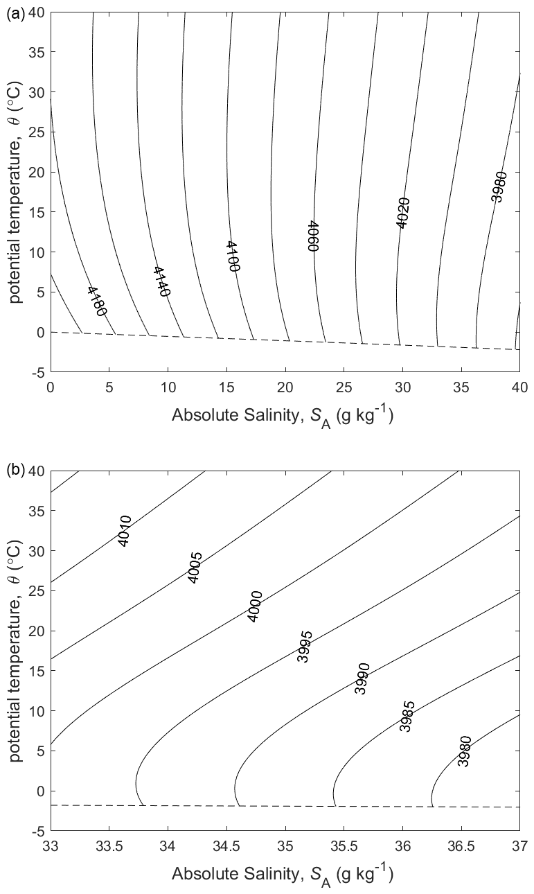
Figure 1 (a) Contours of the isobaric specific heat capacity c_p of seawater (in J kg⁻¹ K⁻¹) at p=0 dbar. (b) A zoomed-in version for a smaller range of Absolute Salinity. The dashed line is the freezing line at p=0 dbar.

With the development of a Gibbs function for seawater, based on empirical fits to measurements of known thermodynamic properties (Feistel, 2008; IOC et al., 2010), it became possible to apply a more rigorous theory for quasi-equilibrium thermodynamics to study heat content problems in the ocean. As a practical matter, calculations can now be made that allow for an estimate of the magnitude of non-conservative terms in the ocean circulation. By integrating over water depth these production rates can be expressed as an equivalent heat flux per unit area.

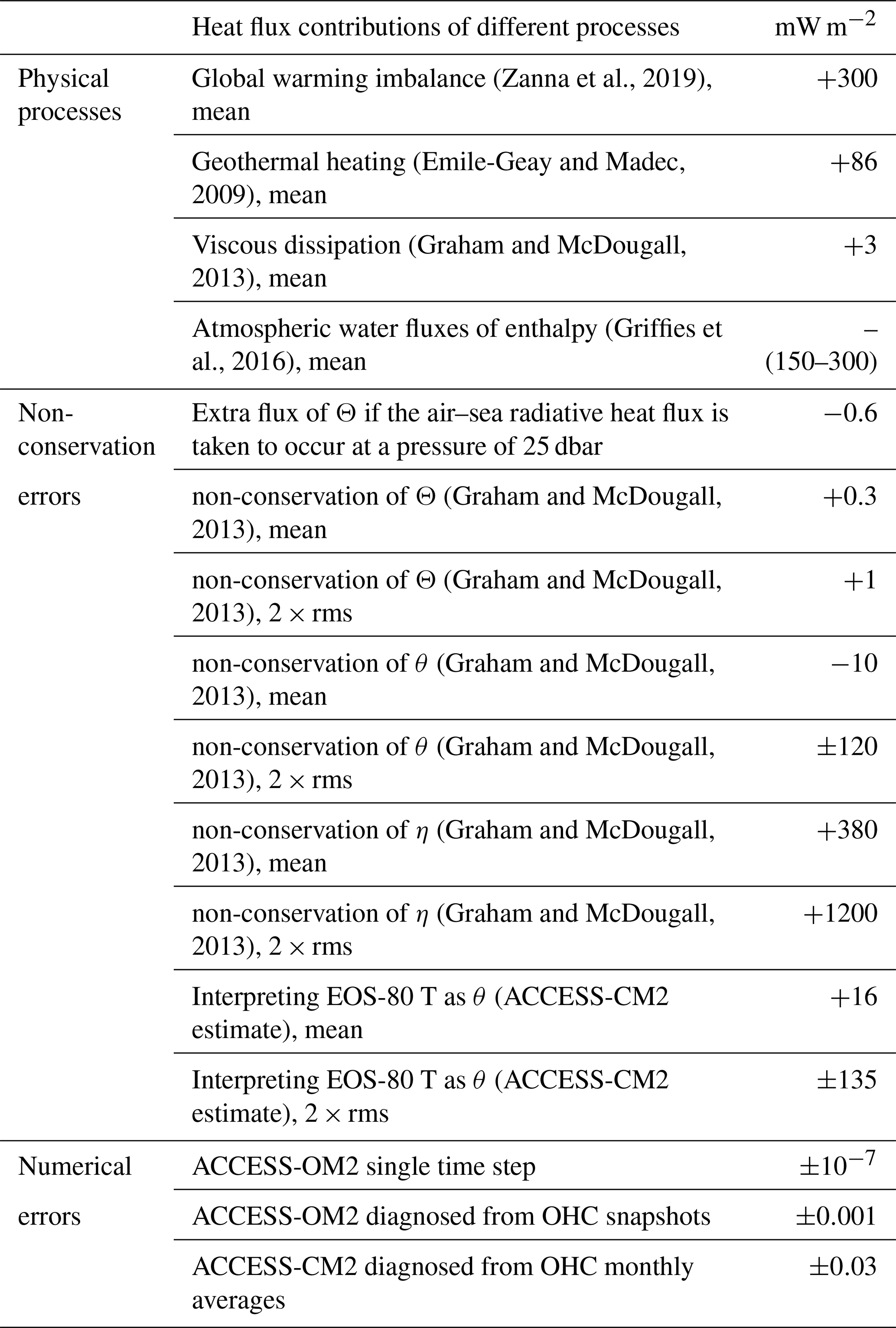
Non-conservation of potential temperature was found to be equivalent to a root mean square surface heat flux of about 60 mW m⁻² (Graham and McDougall, 2013) and an average value of 16 mW m⁻² (see below). These numbers can be compared to a present-day estimated global-warming surface heat flux imbalance of between 300 and 470 mW m⁻² (Zanna et al., 2019; von Schuckmann et al., 2020). By comparison, the globally averaged rate of increase in temperature due to the dissipation of kinetic energy is equivalent to a surface flux of approximately 10 mW m⁻². These equivalent heat fluxes and subsequent similar values are gathered into Table 1 for reference. In the context of a conceptual ocean model being driven by known heat fluxes, the presence of the non-conservation of potential temperature causes sea surface temperature (SST) errors seasonally in the equatorial region of about 0.5 K (0.5 ^∘C), while the error (in all seasons) at the outflow of the Amazon is 1.8 K (see Sect. 9 of McDougall, 2003). With different boundary conditions (such as restoring boundary conditions) the error in assuming that potential temperature is conservative is split in different proportions between (a) the potential temperature values and (b) the potential temperature fluxes.

Table 1 Summary of the impact of various processes and modelling errors on the global ocean heat budget and its imbalance (units: mW m⁻²). Numerical errors are diagnosed from either ACCESS-OM2 (machine precision errors) or ACCESS-CM2 (associated with not having access to OHC snapshots; OHC – ocean heat content). Numbers from interior processes are converted to equivalent surface fluxes by depth integration. The sign convention here is that a positive heat flux is heat entering the ocean or warming the ocean by internal dissipation. The symbol η in this table stands for entropy.

No single alternative thermodynamic variable is available that is both independent of pressure and conservative under mixing. For example, specific entropy is produced in the ocean interior when mixing occurs, with the depth-integrated production being equivalent to an imbalance in the air–sea heat flux of a root mean square value of about 500 mW m⁻² (Graham and McDougall, 2013), while, apart from the dissipation of kinetic energy, enthalpy is conservative under mixing at constant pressure, but enthalpy is intrinsically pressure-dependent.

However, it was found that a constructed variable, potential enthalpy (McDougall, 2003), has a mean non-conservation error in the global ocean of only about 0.3 mW m⁻² (this is the mean value of an equivalent surface heat flux, equal to the depth-integrated interior production of potential enthalpy that is additional to the production due to the dissipation of kinetic energy; Graham and McDougall, 2013). The potential enthalpy, ${\stackrel{\mathrm{̃}}{h}}^{\mathrm{0}}$, is the enthalpy of a water parcel after being moved adiabatically and at constant salinity to the reference pressure 0 dbar at which the temperature is equal to the potential temperature, θ, of the water parcel:

$$\begin{array}{}\text{(1)}& {\stackrel{\mathrm{̃}}{h}}^{\mathrm{0}}\left(S_{\mathrm{A}},\mathit{\theta }\right)=h\left(S_{\mathrm{A}},\mathit{\theta },\mathrm{0}\mathrm{dbar}\right).\end{array}$$

In Eq. (1) the function h is the specific enthalpy of TEOS-10 (defined as a function of Absolute Salinity, in situ temperature, and sea pressure), whereas ${\stackrel{\mathrm{̃}}{h}}^{\mathrm{0}}$ is the potential enthalpy function, and the tilde implies that the temperature input to this function is potential temperature, θ. By way of comparison, the area-averaged geothermal input of heat into the ocean bottom is about 86 mW m⁻², and the interior heating of the ocean due to viscous dissipation, is equivalent to a mean surface heat flux of about 3 mW m⁻² (Graham and McDougall, 2013). Remi Tailleux (personal communication, 2021) has suggested that the dissipation of kinetic energy in the ocean may be as much as 3 times as large as this value at approximately 10 mW m⁻². Thus, we conclude that potential enthalpy, although not a theoretically ideal conservative parameter, can be treated as such for many present purposes in oceanography. If at some stage in the future a source term were to be added to the evolution equation for Conservative Temperature, the most important contribution would be that due to the dissipation of kinetic energy, being a factor of ∼10–30 larger than the non-conservation of Conservative Temperature due to other diffusive contributions (namely the terms in the last two lines of Eq. 38 of Graham and McDougall, 2013).

Since potential enthalpy was not a widely understood property, a decision was made in the development of TEOS-10 to adopt Conservative Temperature, Θ, which has units of temperature and is proportional to potential enthalpy:

$$\begin{array}{}\text{(2)}& \mathrm{\Theta }=\stackrel{\mathrm{̃}}{\mathrm{\Theta }}\left(S_{\mathrm{A}},\mathit{\theta }\right)={\stackrel{\mathrm{̃}}{h}}^{\mathrm{0}}\left(S_{\mathrm{A}},\mathit{\theta }\right)/c_p^{\mathrm{0}},\end{array}$$

where the proportionality constant $c_p^{\mathrm{0}}\equiv \mathrm{3991.867}\mathrm{957}\mathrm{119}\mathrm{63}$ J kg⁻¹ K⁻¹ was chosen so that the average value of Conservative Temperature at the ocean surface matched that of potential temperature. Although in hindsight other choices (e.g. with fewer significant digits) might have been more useful, this value of $c_p^{\mathrm{0}}$ is now built into the TEOS-10 standard.

Note that at specific locations in the ocean, in particular at low salinities and high temperatures, Θ and θ can differ by more than 1 ^∘C (Fig. 2); the difference is a strongly nonlinear function of temperature and salinity. Θ is, by definition, independent of adiabatic and isohaline changes in pressure.

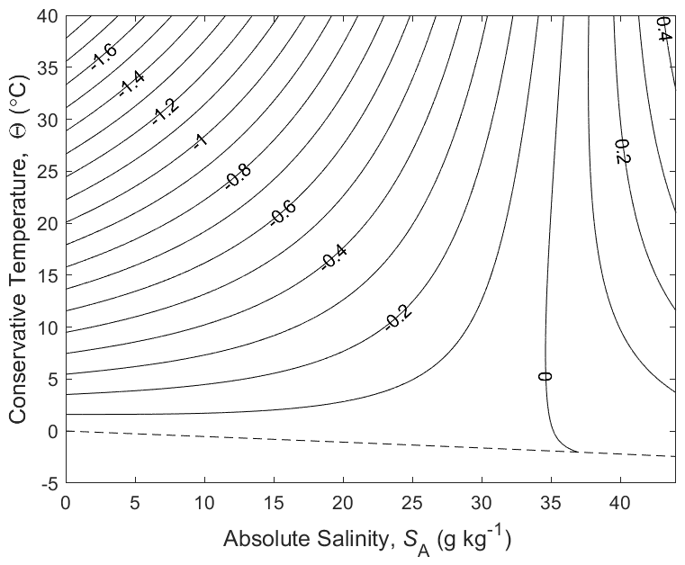
Figure 2 Contours (in ^∘C) of the difference between potential temperature and Conservative Temperature, θ−Θ.

2.2 Why is potential temperature not conservative?

This question is answered in Sects. A17 and A18 of the TEOS-10 manual (IOC et al., 2010) as well as McDougall (2003) and Graham and McDougall (2013). The answer is that potential enthalpy referenced to the sea surface pressure, h⁰, which is a variable that is (almost totally) conservative in the real ocean, is not simply a linear function of potential temperature, θ, and Absolute Salinity, S_A (and note that both enthalpy and entropy are unknown and unknowable up to separate linear functions of Absolute Salinity). If potential enthalpy were a linear function of potential temperature and Absolute Salinity then the “heat content” per unit mass of seawater could be accurately taken to be proportional to potential temperature, and the isobaric specific heat capacity at zero sea pressure would be a constant. As an example of the nonlinearity of ${\stackrel{\mathrm{̃}}{h}}^{\mathrm{0}}(S_{\mathrm{A}},\mathit{\theta })$, the isobaric specific heat at the sea surface pressure $c_p(S_{\mathrm{A}},\mathit{\theta },\mathrm{0}\mathrm{dbar})\equiv h_{\mathit{\theta }}^{\mathrm{0}}$ varies by 6 % across the full range of temperatures and salinities found in the world ocean (Fig. 1). By way of contrast, the potential enthalpy of an ideal gas is proportional to its potential temperature.

Another way of treating heat in an ocean model is to continue carrying potential temperature as its temperature variable but to (i) use the variable isobaric heat capacity at the sea surface to relate the air–sea heat flux to an air–sea flux of potential temperature and (ii) to evaluate the non-conservative source terms of potential temperature and add these source terms to the potential temperature evolution equation during the ocean model simulation (Tailleux, 2015).

However, it is not possible to accurately choose the value of the isobaric heat capacity at the sea surface that is needed when θ is the model's temperature variable. This issue arises because of the unresolved variations in the sea surface salinity (SSS) and SST (for example, unresolved rain events that temporarily lower the SSS), together with the nonlinear dependence of the isobaric specific heat on salinity and temperature. Because of such unresolved correlations, the air–sea heat flux would be systematically misestimated. Nor is it possible to accurately estimate the non-conservative source terms of θ in the ocean interior. This problem arises because the source terms are the product of a turbulent flux and a mean gradient. In a mesoscale eddy-resolved ocean model (or even finer scale) it is not clear how to find the eddy flux of θ, as this depends on how the averaging is done in space and time. Furthermore, when analysing the output of such an ocean model, one would need to find a way of dealing with the contributions from source terms that are not expressible in the form of flux convergences when, for example, estimating the meridional heat transport.

We conclude that the idea that ocean models could retain potential temperature θ as the model's temperature variable, rather than adopt the TEOS-10 recommendation of using Conservative Temperature Θ, is unworkable because (1) the air–sea heat flux cannot be accurately evaluated, (2) the non-conservative source terms that appear in the θ evolution equation cannot be estimated accurately, and (3) the ocean section-integrated heat fluxes cannot be accurately calculated. When contemplating upgrading ocean model physics, rather than retaining the EOS-80 and treating the temperature variable as being potential temperature and having to add estimates of the non-conservative production terms to the temperature evolution equation, it is clearly much simpler and more accurate to instead adopt the TEOS-10 equation of state and to treat the model's temperature variable as Conservative Temperature, as recommended by IOC et al. (2010).

2.3 How conservative is Conservative Temperature?

This question is addressed in McDougall (2003), in Sect. A18 of the TEOS-10 manual (IOC et al., 2010), and in Graham and McDougall (2013). The first step in addressing the non-conservation of Θ is to find a thermophysical variable that is conserved when fluid parcels mix. McDougall (2003) and Graham and McDougall (2013) showed that when fluid parcels are brought together adiabatically and isentropically to mix at pressure p^m, it is the potential enthalpy h^m referenced to the pressure p^m of a mixing event that is conserved, apart from the dissipation of kinetic energy, ε. From this knowledge they constructed the evolution equation for Conservative Temperature (as well as for potential temperature and for entropy).

By contrast, Tailleux (2010, 2015) assumed that it was the total energy, being the sum of internal energy, kinetic energy, and geopotential, that is conserved when fluid parcels mix in the ocean. However, as shown by McDougall et al. (2003), the $-\mathrm{\nabla }\cdot \left(Pu\right)$ term on the right-hand side of the evolution equation for total energy is non-zero when integrated over the mixing region so that total energy is not a conservative variable. For a variable to possess the “conservative property”, it is not sufficient that the material derivative of that property is given by the divergence of a flux. Rather, what is needed is the material derivative of a conservative variable to be equal to the divergence of a flux that is zero in the absence of mixing at that location. That is, the flux whose divergence appears on the right-hand side of the evolution equation of a conservative variable must be a diffusive flux (whether a molecular or a turbulent type of diffusive flux). This feature allows one to integrate over a region in which a mixing event is occurring and be confident that there is no flux through the bounding area that lies outside the fluid that is being mixed. This is not possible for Total Energy because even when integrating out to a quiescent surface that encloses an isolated patch of turbulent mixing, the flux divergence term $-\mathrm{\nabla }\cdot \left(Pu\right)$ can still be non-zero there. Note that both contraction-on-mixing and wave processes contribute to $-\mathrm{\nabla }\cdot \left(Pu\right)$.

Tailleux (2010, 2015) treated this non-conservative term, $-\mathrm{\nabla }\cdot \left(Pu\right)$, as though it were a conservative term in all their evolution equations, so these papers actually arrived at the correct evolution equations for Θ, θ, and η (for example, Eq. B7 of Tailleux, 2010, and Eq. B10 of Graham and McDougall, 2013, are identical). However, these equations were written in terms of the molecular fluxes of heat and salt, and the Tailleux (2010, 2015) papers did not find a way to use these expressions to evaluate the non-conservation of Θ, θ, and η in a turbulently mixed ocean. This was done in Sect. 3 of Graham and McDougall (2013).

While enthalpy is conserved when mixing occurs at constant pressure, it does not possess the “potential” property; rather, an adiabatic and isohaline change in pressure causes a change in enthalpy according to ${\widehat{h}}_P=v$, where v is the specific volume. This property is illustrated in Fig. 3 where it is seen that for an adiabatic and isohaline increase in pressure of 1000 dbar, the increase in enthalpy is the same as that caused by an increase in Conservative Temperature of more than 2.4 ^∘C. If enthalpy variations at constant pressure were a linear function of Absolute Salinity and Conservative Temperature, the contours in Fig. 3 would be parallel equidistant straight lines, and Conservative Temperature would be totally conservative. Since this is not the case, this figure illustrates the (small) non-conservation of Conservative Temperature. Further discussion and evaluation of the non-conservation of Conservative Temperature can be found in McDougall (2003) and Graham and McDougall (2013).

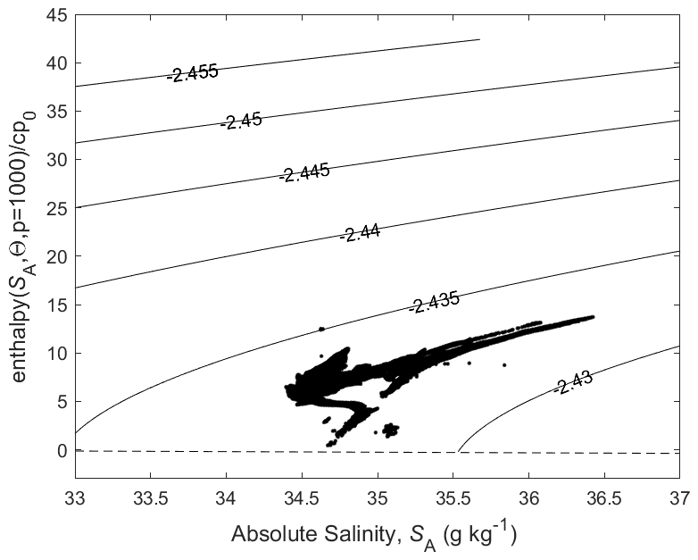
Figure 3 Contours of $\mathrm{\Theta }-\widehat{h}(S_{\mathrm{A}},\mathrm{\Theta },\mathrm{1000}\mathrm{dbar})/c_p^{\mathrm{0}}$ on the Absolute Salinity – $\widehat{h}(S_{\mathrm{A}},\mathrm{\Theta },\mathrm{1000}\mathrm{dbar})c_p^{\mathrm{0}}$ diagram. Enthalpy, $\widehat{h}(S_{\mathrm{A}},\mathrm{\Theta },\mathrm{1000}\mathrm{dbar})$, is a conservative quantity for turbulent mixing processes that occur at a pressure of 1000 dbar. The mean value of the contoured quantity is approximately −2.44 ^∘C, illustrating that enthalpy does not possess the “potential” property; that is, enthalpy increases during adiabatic and isohaline increases in pressure. The fact that the contoured quantity in this figure is not a linear function of S_A and $\widehat{h}(S_{\mathrm{A}},\mathrm{\Theta },\mathrm{1000}\mathrm{dbar})$ illustrates the (small) non-conservative nature of Conservative Temperature. The dots are data from the world ocean at 1000 dbar.

2.4 Seawater salinity

To a degree of approximation which is useful for many purposes, the dissolved matter in seawater (“sea salt”) can be treated as a material of uniform composition, whose globally integrated absolute salinity (i.e. the grams of solute per kilogram of seawater) changes only due to the addition and removal of fresh water through rain, evaporation, and river inflow. This property is because the processes that govern the addition and removal of the constituents of sea salt have extremely long timescales relative to those that affect the pure water component of seawater. We can thus treat the total ocean salt content as approximately constant but subject to spatially and temporally varying boundary fluxes of fresh water that give rise to salinity gradients.

The utility of this definition of uniform composition of sea salt lies in its conceptual simplicity, which is well-suited to theoretical and numerical ocean modelling at timescales of up to hundreds of years. However, to the demanding degree required for observing and understanding deep-ocean pressure gradients, sea salt is neither uniform in composition nor a conserved variable, and its absolute amount cannot be measured precisely in practice. The repeatable precision of various technologies used to estimate salinity can be as small as 0.002 g kg⁻¹, but the non-ideal nature of seawater means that these estimates can be different by as much as 0.025 g kg⁻¹ relative to the true Absolute Salinity in the open ocean, and as much 0.1 g kg⁻¹ in coastal areas (Pawlowicz, 2015).

The most important interior source and sink factors governing changes in the composition of sea salt are biogeochemical processes that govern the biological uptake of dissolved nutrients, calcium, and carbon in the upper ocean, as well as the remineralization of these substances from sinking particles at depth. At present it is thought that changes resulting from hydrothermal vent activity, fractionation from sea ice formation, and multi-component molecular diffusion processes are of local importance only, but little work has been done to quantify this.

To address this problem, TEOS-10 defines a Reference Composition of seawater and several slightly different salinity variables that are necessary for different purposes to account for the variable composition of sea salt. The TEOS-10 Absolute Salinity, S_A, is the absolute salinity of Reference Composition Seawater of a measured density (note that capitalization of variable names denotes a precise definition in TEOS-10). It is the salinity variable that is designed to be used to accurately calculate density using the TEOS-10 Gibbs function.

Preformed Salinity, S_*, is the salinity of a seawater parcel with the effects of biogeochemical processes removed, which is somewhat analogous to a chlorinity-based salinity estimate. It is thus a conservative tracer of seawater suitable for modelling purposes, but it neglects the spatially variable small portion of sea salt involved in biogeochemical processes that is required for the most accurate density estimates. Since the original measurements of specific volume to which both EOS-80 and TEOS-10 were fitted were made on samples of Standard Seawater with a composition close to the Reference Composition, the Reference Salinity of these samples is also the same as Preformed Salinity.

Ocean observational databases contain a completely different variable: Practical Salinity. This variable, which predates TEOS-10, is essentially based on a measure of the electrical conductance of seawater normalized to conditions of fixed temperature and pressure by empirical correlation equations between the ranges of 2 and 42 PSS-78 and scaled so that ocean salinity measurements that have been made through a variety of technologies over the past 120 years are numerically comparable. Practical Salinity measurement technologies involve a certified reference material called IAPSO Standard Seawater, which for our purposes can be considered the best available artefact representing seawater of Reference Composition.

Practical Salinity was not designed for numerical modelling purposes and does not accurately represent the mass fraction of dissolved matter. We can link Practical Salinity, S_P, to the Absolute Salinity of Reference Composition seawater (so-called Reference Salinity, S_R) using a fixed scale factor, u_PS, so that

$$\begin{array}{}\text{(3)}& S_{\mathrm{R}}=u_{\mathrm{PS}}{S}_P\mathrm{where}{u}_{\mathrm{PS}}\equiv (\mathrm{35.165}\mathrm{04}/\mathrm{35})\mathrm{g}{\mathrm{kg}}^{-\mathrm{1}}.\end{array}$$

Conversions to and between the other “salinity” definitions, however, involve knowledge about spatial and temporal variations in seawater composition. Fortunately, the largest component of these changes occurs in a set of constituents involved in biogeochemical processes, whose co-variation is known to be strongly correlated. Thus, the Absolute Salinity of real seawater can be determined globally to useful accuracy from the Reference Salinity by the addition of a single parameter: the so-called Absolute Salinity Anomaly, δS_A,

$$\begin{array}{}\text{(4)}& S_{\mathrm{A}}=S_{\mathrm{R}}+\mathit{\delta }{S}_{\mathrm{A}},\end{array}$$

which has been tabulated in a global atlas for the current ocean (McDougall et al., 2012) and is estimated in coastal areas by considering the effects of river salts (Pawlowicz, 2015). It can also be determined from measurements of either density or of carbon and nutrients (IOC et al., 2010; Ji et al., 2021). For the purposes of numerical ocean modelling, the Absolute Salinity Anomaly could in theory be obtained by separately tracking the carbon cycle and nutrients and applying known correction factors, but we are not aware of any attempts to do so.

Chemical modelling (Pawlowicz, 2010; Pawlowicz et al., 2011; Wright et al., 2011; Pawlowicz et al., 2012) suggests the approximate relation

$$\begin{array}{}\text{(5)}& S_{\mathrm{A}}-S_{*}\approx \mathrm{1.35}\mathit{\delta }{S}_{\mathrm{A}}\equiv \mathrm{1.35}\left(S_{\mathrm{A}}-S_{\mathrm{R}}\right),\end{array}$$

and these relationships are schematically illustrated in Fig. 4. The magnitude of the Absolute Salinity Anomaly is around −0.005 to +0.025 g kg⁻¹ in the open ocean relative to a mean Absolute Salinity of about 35 g kg⁻¹. The correction it implies may be important when initializing models or comparing them with observations, but its major effect is likely in producing biases in calculated isobaric density gradients.

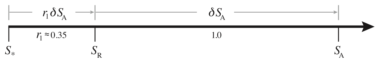
Figure 4 Number line of salinity, illustrating the differences between Preformed Salinity S_*, Reference Salinity S_R, and Absolute Salinity S_A for seawater whose composition differs from that of Standard Seawater which has Reference Composition. If a seawater sample has Reference Composition, then δS_A=0 and S_*, S_R and S_A are all equal.

2.5 Seawater density

The density of seawater is the most important thermodynamic property affecting oceanic motions, since its spatial changes (along with changes to the sea surface height) give rise to pressure gradients which are the primary driving force for currents within the ocean interior through the hydrostatic relation. The “traditional” equation of state is known as EOS-80 (UNESCO, 1981) and is standardized as a function of Practical Salinity and in situ temperature, $\mathit{\rho }=\mathit{\rho }(S_P,t,p)$, which has 41 numerical terms. An additional equation (the adiabatic lapse rate) is required for conversion of temperature to potential temperature. However, for ocean models, the EOS-80 is usually taken to be the 41-term expression written in terms of potential temperature, $\mathit{\rho }=\stackrel{\mathrm{̃}}{\mathit{\rho }}(S_P,\mathit{\theta },p)$, of Jackett and McDougall (1995), where the tilde indicates that this rational function fit was made with Practical Salinity S_P and potential temperature θ as the input salinity and temperature variables.

The current standard for describing the thermodynamic properties of seawater, known as TEOS-10, provides an equation of state, $v=\mathrm{1}/\mathit{\rho }=v(S_{\mathrm{A}},t,p)$, in the form of a function which involves 72 coefficients (IOC et al., 2010) and is an analytical pressure derivative of the TEOS-10 Gibbs function. However, for ocean models using TEOS-10 the equation of state used is one of those in Roquet et al. (2015): the 55-term equation of state, $\mathit{\rho }=\widehat{\mathit{\rho }}(S_{\mathrm{A}},\mathrm{\Theta },z)$, used by Boussinesq models and the 75-term polynomial for specific volume, $v=\widehat{v}(S_{\mathrm{A}},\mathrm{\Theta },p)$, used by non-Boussinesq ocean models.

In this paper we will not concentrate on the distinction between Boussinesq and non-Boussinesq ocean models, and henceforth we will take the third input to the equation of state to be pressure, even though for a Boussinesq model it is in fact a scaled version of depth as per the energetic arguments of Young (2010). By the same token, we will cast the discussion in terms of the in situ density, even though the non-Boussinesq models have as their equation of state a polynomial for the specific volume, $v=\mathrm{1}/\mathit{\rho }$.

For seawater of Reference Composition, both the TEOS-10 and EOS-80 fits $\mathit{\rho }=\widehat{\mathit{\rho }}(S_{\mathrm{A}},\mathrm{\Theta },p)$ and $\mathit{\rho }=\stackrel{\mathrm{̃}}{\mathit{\rho }}(S_P,\mathit{\theta },p)$ are almost equally accurate (see Sect. A5 of IOC et al., 2010, and note the comparison between Figs. A5.1 and A5.2 therein). That is, if we set δS_A=0 and use Eq. (3) to relate Practical and Reference Salinities (which in this case are the same as Preformed Salinities), the numerical density values of in situ density calculated using EOS-80 are not significantly different to those using TEOS-10 in the open ocean (the differences are significant for brackish waters).

This being the case, we can see from Sects. A5 and A20 of the TEOS-10 manual (IOC et al., 2010) that 58 % of the data deeper than 1000 dbar in the world ocean would have the thermal wind misestimated by ∼2.7 % due to ignoring the difference between Absolute and Reference Salinities. No ocean model has addressed this deficiency to date, but McCarthy et al. (2015) studied the influence of using Absolute Salinity versus Reference Salinity in calculating the overturning circulation in the North Atlantic. They found that the overturning stream function changed by 0.7 Sv at a depth of 2700 m relative to a mean value at this depth of about 7 Sv, i.e. a 10 % effect. Because we argue that the salinity variable in ocean models is best interpreted as being Preformed Salinity, S_*, the neglect of the distinction between Preformed and Absolute Salinities in ocean models means that they misestimate the overturning stream function by 1.35 (see Fig. 4) times 0.7 Sv, namely ∼1 Sv, i.e. a 13.5 % effect.

2.6 Air–sea heat fluxes

Sensible, latent, and longwave radiative fluxes are affected by near-surface turbulence and are usually calculated using bulk formulae involving air and sea surface water temperatures (the air and sea in situ temperatures), as well as other parameters (e.g. the latent heat involves the isobaric evaporation enthalpy, commonly called the latent heat of evaporation, which is actually a weak function of temperature and salinity; see Eq. 6.28 of Feistel et al., 2010, and Eq. 3.39.7 of IOC et al., 2010). The total air–sea heat flux, Q, is then translated into a water temperature change by dividing by a heat capacity $c_p^{\mathrm{0}}$, which has always been taken to be constant in numerical models (Griffies et al., 2016). Although this method is appropriate for Conservative Temperature, CT (assuming that the TEOS-10 value is used for $c_p^{\mathrm{0}}$), it is not appropriate when potential temperature is being considered. The flux of potential temperature into the surface of the ocean should be Q divided by $c_p(S_{*},\mathit{\theta },\mathrm{0})$. The use of a constant specific heat capacity, in association with the interpretation of the ocean's temperature variable as being potential temperature, means that the ocean has received a different amount of heat than the atmosphere actually delivers to the ocean, and this issue will be explored in Sect. 3.

When precipitation (P) occurs at the sea surface, this addition of fresh water brings with it the associated potential enthalpy $h(S_{\mathrm{A}}=\mathrm{0},t,\mathrm{0}\mathrm{dbar})$ per unit mass of fresh water, where t is the in situ temperature of the raindrops as they arrive at the sea surface. The temperature at which rain enters the ocean is not yet treated consistently in coupled models, and Sect. K1.6 of Griffies et al. (2016) suggests that this effect could be equivalent to an area-averaged extra air–sea heat flux of between −150 and −300 mW m⁻², representing a heat loss for the ocean.

2.7 Numerical ocean models

In deciding how to numerically model the ocean, an explicit choice must be made about the equation of state, and one would think that this choice would have implications about the precise meaning of the temperature and salinity variables in the model, which we will call T_model and S_model, respectively. We can divide ocean models into two general classes: EOS-80 models and TEOS-10 models.

2.7.1 EOS-80 models

One class of CMIP ocean model is based around EOS-80, and these models have the following characteristics.

1. The model's equation of state, $\mathit{\rho }=\stackrel{\mathrm{̃}}{\mathit{\rho }}(S_P,\mathit{\theta },p)$, expects to have Practical Salinity and potential temperature as the salinity and temperature input parameters.

2. T_model is advected and diffused in the ocean interior in a conservative manner; i.e. its evolution at a point in space is determined by the convergence of advective fluxes plus parameterized sub-grid-scale diffusive and skew diffusive fluxes.

3. S_model is advected and diffused in the ocean interior in a conservative manner as for T_model.

4. The air–sea heat flux is delivered to and from the ocean using a constant isobaric specific heat, $c_p^{\mathrm{0}}$, to convert the air–sea heat flux into a surface flux of T_model. (An EOS-80-based model's value of $c_p^{\mathrm{0}}$ is generally only slightly different to the TEOS-10 value.)

5. T_model is initialized from an atlas of values of potential temperature, and S_model is initialized with values of Practical Salinity.

At first glance, it seems reasonable to assume that T_model is potential temperature and S_model is Practical Salinity. However, these assumptions imply that theoretical errors arising from items 2, 3, and 4 are ignored (since neither potential temperature nor Practical Salinity is a conservative variable). In this paper we show that these interpretations of the model's temperature and salinity variables are not as accurate as our proposed alternative interpretations.

2.7.2 TEOS-10 models

Other ocean models have begun to implement TEOS-10 features. These models generally have the following characteristics.

1. The model's equation of state, $\mathit{\rho }=\widehat{\mathit{\rho }}(S_{\mathrm{A}},\mathrm{\Theta },p)$, expects to have Absolute Salinity and Conservative Temperature as its salinity and temperature input parameters.

2. T_model is advected and diffused in the ocean interior in a conservative manner.

3. S_model is advected and diffused in the ocean interior in a conservative manner.

4. At each time step of the model, the value of potential temperature at the sea surface (i.e. SST) is calculated from the T_model (which is assumed to be Conservative Temperature), and this value of SST is used to interact with the atmosphere via bulk flux formulae.

5. The air–sea heat flux is delivered to and from the ocean using the TEOS-10 constant isobaric specific heat, $c_p^{\mathrm{0}}$, to convert the air–sea heat flux into a surface flux of T_model.

6. T_model is initialized from an atlas of values of Conservative Temperature, and S_model is initialized with values of one of Absolute Salinity, Reference Salinity, or Preformed Salinity.

Implicitly, it has then been assumed that T_model is a Conservative Temperature and S_model is Absolute Salinity.

There is one CMIP6 ocean model that we are aware of, ACCESS-CM2 (Australian Community Climate and Earth System Simulator; Bi et al., 2020), whose equation of state is written in terms of Conservative Temperature, but the salinity argument in the equation of state is Practical Salinity. The salinity in this model is initialized with atlas values of Practical Salinity.

From the above it is clear that there are small but significant theoretical incompatibilities between different models and between models and the observed ocean. These issues become apparent when dealing with the technicalities of intercomparisons, and various choices must be made. We now consider the implications of these different choices and provide recommendations for best practices.

3 The interpretation of salinity in ocean models

Note that the samples whose measured specific volumes were incorporated into both the EOS-80 and TEOS-10 equations of state were of Standard Seawater whose composition is close to Reference Composition. Consequently, the EOS-80 and TEOS-10 equations of state were constructed with Preformed Salinity, S_* (or, in the case of EOS-80 models, $S_{*}/u_{\mathrm{PS}}$), as their salinity arguments, not Reference Salinity. These same algorithms give accurate values of specific volume for seawater samples that are not of Reference Composition so long as the salinity argument is Absolute Salinity (as opposed to Reference Salinity or Preformed Salinity).

For an ocean model that has no non-conservative interior source terms affecting the evolution of its salinity variable and that is initialized at the sea surface with Preformed Salinity, the only interpretation for the model's salinity variable is Preformed Salinity, and the use of the TEOS-10 equation of state will then yield the correct specific volume. Furthermore, whether the model is initialized with values of Absolute Salinity, Reference Salinity, or Preformed Salinity, these initial salinity values are nearly identical in the upper ocean, and any differences between the three initial conditions in the deeper ocean would be largely diffused away within the long spin-up period. That is, in the absence of the non-conservative biogeochemical source terms that would be needed to model Absolute Salinity and to force it away from being conservative (or the smaller source terms that would be needed to maintain Reference Salinity), the model's salinity variable will drift towards being Preformed Salinity. Hence, we conclude that, after the long spin-up phase, the salinity variable of a TEOS-10-based ocean model is accurately interpreted as being preformed salinity S_*, irrespective of whether the model was initialized with values of Absolute Salinity, Reference Salinity, or Preformed Salinity.

Likewise, the prognostic salinity variable after a long spin-up period of an EOS-80-based model is most accurately interpreted as being Preformed Salinity divided by $u_{\mathrm{PS}}\equiv (\mathrm{35.165}\mathrm{04}/\mathrm{35})$ g kg⁻¹, $S_{*}/u_{\mathrm{PS}}$.

We clearly need more estimates of the magnitude of the dynamic effects of the variable seawater composition, but for now we might take a change in 1 Sv in the meridional transport of deepwater masses in each ocean basin (based on the Atlantic work of McCarthy et al., 2015) as an indication of the magnitude of the effect of neglecting the effects of biogeochemistry on salinity. At this stage of model development, since all models are equally deficient in their thermophysical treatment of salinity, at least this aspect does not present a problem as far as making comparisons between CMIP models.

4 Model heat flux calculations

From the details described above, both types of numerical ocean models suffer from some internal contradictions with thermodynamical best practice. For example, for the EOS-80-based models, if T_model is assumed to be potential temperature, the use of EOS-80 is correct for density calculations but the use of conservative equations for T_model ignores the non-conservative production of potential temperature. The use of a constant heat capacity is also in error if T_model is interpreted as potential temperature. Conservative equations are, however, appropriate for Conservative Temperature. In addition, if S_model is assumed to be either Practical Salinity or Absolute Salinity, then the use of conservative equations ignores the changes in salinity that arise from biogeochemical processes.

One use for these models is to calculate heat budgets and heat fluxes – both at the surface and between latitudinal bands, and inherent to CMIP is the idea that these different models should be intercompared. The question of how this intercomparison should be done, however, was not clearly addressed in Griffies et al. (2016). Here we begin the discussion by considering two different options for interpreting T_model in EOS-80 ocean models.

4.1 Option 1: interpreting the EOS-80 model's temperature as being potential temperature

Under this option the model's temperature variable T_model is treated as being potential temperature θ; this is the prevailing interpretation to date. With this interpretation of T_model one wonders whether Conservative Temperature Θ should be calculated from the model's (assumed) potential temperature before calculating (i) the global Ocean Heat Content as the volume integral of $\mathit{\rho }{c}_p^{\mathrm{0}}\mathrm{\Theta }$ and (ii) the advective meridional heat transport as the area integral of $\mathit{\rho }{c}_p^{\mathrm{0}}\mathrm{\Theta }v$ at constant latitude, where v is the northward velocity. This question was not clearly addressed in Griffies et al. (2016), and here we emphasize one of the main conclusions of the present paper, namely that ocean heat content and meridional heat transports should be calculated using the model's prognostic temperature variable. Any subsequent conversion from one temperature variable to another (such as potential to conservative) in order to calculate heat content and heat transport is incorrect and confusing and should not be attempted.

4.1.1 Issues with the potential temperature interpretation

There are several thermodynamic inconsistencies that arise from option 1. First, the ocean model has assumed in its spin-up phase (for perhaps a millennium) that T_model is conservative, so during the whole spin-up phase and beyond, the contribution of the known non-conservative interior source terms of potential temperature has been absent, and hence the model's temperature variable has not responded to these absent source terms, so this temperature field cannot be potential temperature. Also, since the temperature field of the model is not potential temperature (because of these absent source terms) the velocity field of the model will also not be forced correctly due to errors in the density field, which in turn affect the pressure force.

The second inconsistent aspect of option 1 is that the air–sea flux of heat is ingested into the ocean model during both the spin-up stage and the subsequent transient response phase, as though the model's temperature variable is proportional to potential enthalpy. For example, consider some time during the year at a particular location where the sea surface is fresh (a river outflow or melted ice). During this time, any heat that the atmosphere loses or gains should have affected the potential temperature of the upper layers of the ocean using a specific heat that is 6 % larger than $c_p^{\mathrm{0}}$ (see Fig. 1). So, if the ocean model's temperature variable is interpreted as being potential temperature, a 6 % error is made in the heat flux that is exchanged with the atmosphere during these periods and at these locations. That is, the changes in the ocean model's (assumed) potential temperature caused by the air–sea heat flux will be exaggerated where and when the sea surface salinity is fresh. This 6 % flux error is not corrected by subsequently calculating Conservative Temperature from potential temperature; for example, these temperatures are the same at low temperature and salinity (see Fig. 2), and yet at low values of salinity, the specific heat is 6 % larger than $c_p^{\mathrm{0}}$.

This second inconsistent aspect of option 1 can be restated as follows. The adoption of potential temperature as the model's temperature variable means that there is a discontinuity in the heat flux of the coupled air–sea system right at the sea surface; for every Joule of heat (i.e. potential enthalpy) that the atmosphere gives to the ocean, under this option 1 interpretation, up to 6 % too much heat arrives in the ocean over relatively fresh waters. In this way, the adoption of potential temperature as the model temperature variable ensures that the coupled ocean–atmosphere system will not conserve heat. Rather, there appear to be non-conservative sources and sinks of heat right at the sea surface where heat is unphysically manufactured or destroyed.

The third inconsistent aspect is a direct consequence of the second; namely, if one is tempted to post-calculate Conservative Temperature Θ from the model's (assumed) values of potential temperature, the rate of change of the calculated ocean heat content as the volume integral of $\mathit{\rho }{c}_p^{\mathrm{0}}\mathrm{\Theta }$ would no longer be accurately related to the heat that the atmosphere exchanged with the ocean. Nor would the area integral between latitude bands of the air–sea heat flux be exactly equal to the difference between the calculated oceanic meridional heat transports that cross those latitudes. Rather, during the running of the model the heat that was lost from the atmosphere actually shows up in the ocean as the volume integral of the model's prognostic temperature variable. Thus, we agree with Appendix D3.3 of Griffies et al. (2016) and strongly recommend that Conservative Temperature not be calculated a posteriori in order to evaluate heat content and heat fluxes in these EOS-80-based models.

4.1.2 Quantifying the air–sea flux imbalance

Here we quantify the air–sea flux errors involved with assuming that T_model of EOS-80 models is potential temperature. These EOS-80-based models calculate the air–sea flux of their model's temperature as the air–sea heat flux, Q, divided by $c_p^{\mathrm{0}}$. However, since the isobaric specific heat capacity of seawater at 0 dbar is $c_p(S_{*},\mathit{\theta },\mathrm{0})$, the flux of potential temperature into the surface of the ocean should be Q divided by $c_p(S_{*},\mathit{\theta },\mathrm{0})$. So, if the model's temperature variable is interpreted as being potential temperature, the EOS-80 model has a flux of potential temperature entering the ocean that is too large by the difference between these fluxes, namely by $Q/c_p^{\mathrm{0}}$ minus $Q/c_p(S_{*},\mathit{\theta },\mathrm{0})$. This means that the ocean has received a different amount of heat than the atmosphere actually delivers to the ocean, with the difference, ΔQ, being $c_p(S_{*},\mathit{\theta },\mathrm{0})$ times the difference in the surface fluxes of potential temperature, namely (for the last part of this equation, see Eq. A12.3a of IOC et al., 2010)

$$\begin{array}{}\text{(6)}& \mathrm{\Delta }Q=Q\left({\displaystyle \frac{c_p\left(S_{*},\mathit{\theta },\mathrm{0}\right)}{c_p^{\mathrm{0}}-\mathrm{1}}}\right)=Q\left({\stackrel{\mathrm{̃}}{\mathrm{\Theta }}}_{\mathit{\theta }}-\mathrm{1}\right).\end{array}$$

We plot this quantity from the pre-industrial control run of ACCESS-CM2 in Fig. 5c and show it as a cell-area-weighted histogram in Fig. 5e (note that while these plots apply to EOS-80-based ocean models, to generate these plots we have actually used data from ACCESS-CM2, which is a mostly TEOS-10-compliant model). The calculation takes into account the penetration of shortwave radiation into the ocean but is performed using monthly averages of the thermodynamics quantities. The temperatures and salinities at which the radiative flux divergences occur are taken into account in this calculation. However, the result is little changed if the sea surface temperatures and salinities are used with the radiative flux divergence assumed to take place at the sea surface. Results from similar calculations performed using monthly and daily averaged quantities in ACCESS-OM2 ocean-only model simulations were similar, suggesting that correlations between sub-monthly variations are not significant in such a relatively coarse-resolution model.

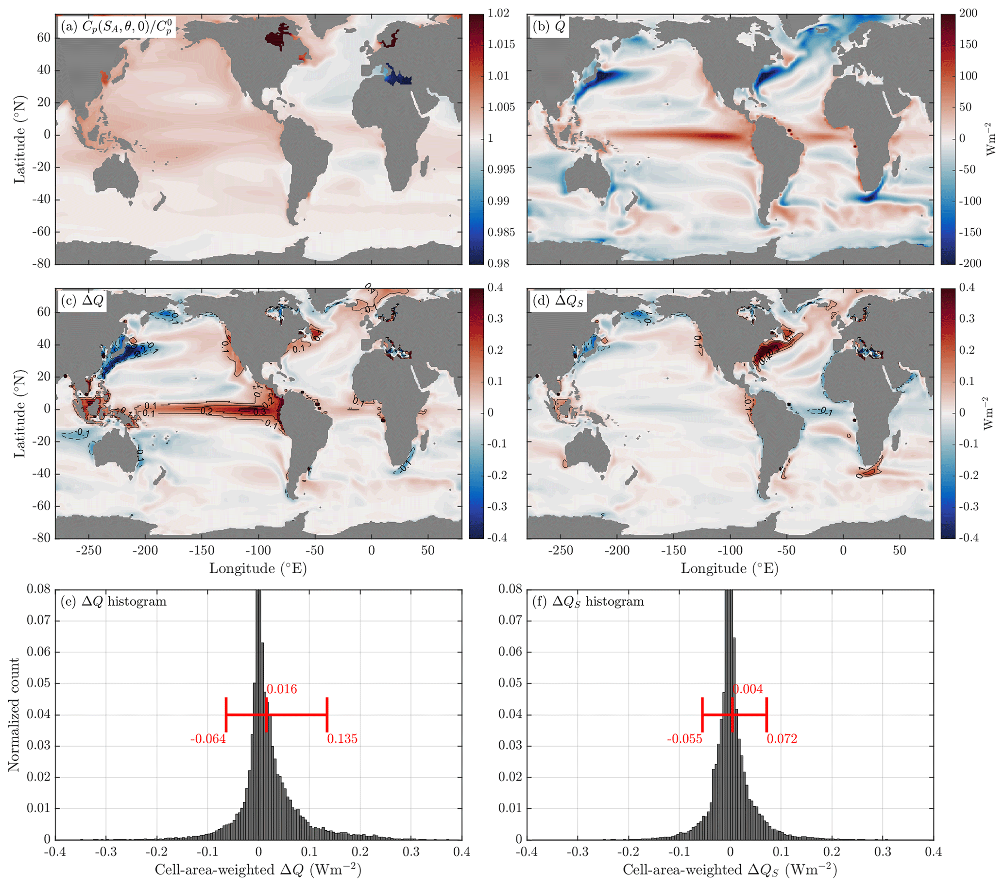
Figure 5 (a) The average value of the ratio of the isobaric specific heat of seawater and $c_p^{\mathrm{0}}$ for data from the ACCESS-CM2 model's pre-industrial control simulation (600 years long). (b) The average surface heat flux Q (W m⁻²) in this same ocean model. (c) The additional heat that the ocean receives or loses compared to the heat that the atmosphere loses or receives (assuming that an EOS-80 model's temperature variable is potential temperature), ΔQ (W m⁻², Eq. 6). (e) A histogram of ΔQ weighted by the area of each grid cell. (d) The contribution of salinity variations to the air–sea heat flux discrepancy given by $\mathrm{\Delta }{Q}_{\mathrm{S}}=Q(S-\stackrel{\mathrm{‾}}{S})(\mathrm{1}/c_p^{\mathrm{0}})\partial c_p/\partial S$, where $\stackrel{\mathrm{‾}}{S}$ is the surface mean salinity and $\partial c_p/\partial S$ is the variation in the specific heat with salinity at the surface mean salinity and potential temperature. (f) A histogram of ΔQ_S weighted by the area of each grid cell. Shown in red in panels (e) and (f) are the mean as well as the 5th and 95th  percentiles of the histogram (W m⁻²). Note that these calculations neglect correlations between surface properties and the surface heat flux at sub-monthly timescales.

ΔQ has an area-weighted mean value of 16 mW m⁻², and we know that this represents the net surface flux of potential temperature required to balance the volume-integrated non-conservation of potential temperature in the ocean's interior (Tailleux, 2015). To put this value in context, 16 mW m⁻² corresponds to 5 % of the observed trend of 300 mW m⁻² in the global ocean heat content from 1955–2017 (Zanna et al., 2019). In addition to this mean value of ΔQ, we see from Fig. 5c that there are regions such as the equatorial Pacific and the western North Pacific where ΔQ is as large as the area-averaged heat flux of 300 mW m⁻² that the ocean has received since 1955. These local anomalies of air–sea flux, if they existed, would drive local variations in temperature. However, these ΔQ values do not represent real heat fluxes. Rather, they represent the error in the air–sea heat flux that we make if we insist that the temperature variable in an EOS-80-based ocean model is potential temperature, with the ocean receiving a surface heat flux that is larger by ΔQ than the atmosphere delivers to the ocean. Figure 6 shows the zonal integration of ΔQ in units of Watts per degree of latitude.

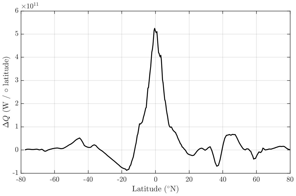
Figure 6 The ACCESS-CM2 zonally integrated ΔQ from Fig. 5c, showing the imbalance in the air–sea heat flux in Watts per degree of latitude.

Figure 5e shows that, with T_model being interpreted as potential temperature, 5 % of the surface area of the ocean needs a surface heat flux that is more than 135 mW m⁻² different to what the atmosphere gives to and from the ocean. This regional variation of ΔQ of approximately ±100 mW m⁻² is consistent with the regional variations in the air–sea flux of potential temperature found by Graham and McDougall (2013) that is needed to balance the depth-integrated non-conservation of potential temperature as a function of latitude and longitude. This damage that is done to the air–sea heat flux at a given horizontal location by the interpretation that the temperature variable of an EOS-80 ocean model is potential temperature is not small in comparison to the globally averaged rate that our planet is being anthropogenically warmed. That is, in regions that are comparable in size to an ocean basin (see Fig. 5c), a heat budget analysis using EOS-80 and potential temperature would find a false trend as large as the globally averaged rate that our planet is warming.

Figure 5d and f show that much of this spread is due to the variation of the isobaric specific heat capacity in salinity, with the remainder due to the variation of this heat capacity with temperature. We note that if this analysis were performed with a model that resolved individual rain showers and the associated freshwater lenses on the ocean surface, then these episodes of very fresh water at the sea surface would be expected to increase the calculated values of ΔQ. Interestingly, by way of contrast, it is the variation of the isobaric heat capacity with temperature that dominates (by a factor of 4) the contribution of this heat capacity variation to the area mean of ΔQ (with the contribution of salinity, ΔQ_S, in Fig. 5d leading to an area mean of 4 mW m⁻²), as originally found by Tailleux (2015).

While a heat flux error of ±100 mW m⁻² is not large, it also not trivially small, and it seems advisable to respect these fundamental thermodynamic aspects of the coupled Earth system. We will see that this ±100 mW m⁻² issue is simply avoided by realizing that the temperature variable in these EOS-80 models is not potential temperature.

In Appendix A we enquire whether the way that EOS-80 models treat their fluid might be made to be thermodynamically correct for a fluid other than seawater. We find that it is possible to construct such a thermodynamic definition of a fluid with the aim that its treatment in EOS-80 models is consistent with the laws of thermodynamics. This fluid has the same specific volume as seawater for given values of salinity, potential temperature, and pressure, but it has different expressions for both enthalpy and entropy. This fluid also has a different adiabatic lapse rate and therefore a different relationship between in situ and potential temperatures. However, this exercise in thermodynamic abstraction does not alter the fact that, as a model of the real ocean and with the temperature variable being interpreted as being potential temperature, the EOS-80 models have ΔQ more heat arriving in the ocean than leaves the atmosphere.

Since CMIP6 is centrally concerned with how the planet warms, it is advisable to adopt a framework wherein heat fluxes and their consequences are respected. That is, we regard it as imperative to avoid non-conservative sources of heat at the sea surface. It is the insistence that the temperature variable in EOS-80-based models is potential temperature that implies that the ocean receives a heat flux from the atmosphere that is larger by ΔQ than what the atmosphere actually exchanges with the ocean. Since there are some areas of the ocean surface where ΔQ is as large as the mean rate of global warming, option 1 is not supportable. This situation motivates option 2 whereby we change the interpretation of the model's temperature variable from being potential temperature to Conservative Temperature even when using EOS-80.

4.2 Option 2: interpreting the EOS-80 model's temperature as being Conservative Temperature

Under this option the ocean model's temperature variable is taken to be Conservative Temperature Θ. The air–sea flux of potential enthalpy is then correctly ingested into the ocean model using the fixed specific heat $c_p^{\mathrm{0}}$, and the mixing processes in the model correctly conserve Conservative Temperature. Hence, the second, fourth, and fifth items listed in Sect. 2 are handled correctly, except for the following caveat. In the coupled model, the bulk formulae that set the air–sea heat flux at each time step use the uppermost model temperature as the sea surface temperature as input. So with the option 2 interpretation of the model's temperature variable as being Conservative Temperature, these bulk formulae are not being fed the SST (which at the sea surface is equal to the potential temperature θ). The difference between these temperatures is Θ−θ, which is the negative of what we plot in Fig. 2. This is a caveat with this option 2 interpretation, namely that the bulk formula that the model uses to determine the air–sea flux at each time step is a little different to what was intended when the parameters of the bulk formulae were chosen. This is a caveat regarding what was intended by the coupled modeller rather than what the coupled model experienced. That is, with this option 2 interpretation, the air–sea heat flux, while being a little bit different than what might have been intended, does arrive in the ocean properly; there is no non-conservative production or destruction of heat at the air–sea boundary as there is in option 1.

Regarding the remaining two items involving temperature listed in Sect. 2, we can dismiss the fifth item, since any small difference in the initial values, set at the beginning of the lengthy spin-up period, between potential temperature and Conservative Temperature will be irrelevant after the long spin-up integration.

This then leaves the first point, namely that the model used the equation of state that expects potential temperature as its temperature input, $\stackrel{\mathrm{̃}}{\mathit{\rho }}(S_{*}/u_{\mathrm{PS}},\mathit{\theta },p)$, but under this option 2 we are interpreting the model's temperature variable as being Conservative Temperature. In the remainder of this section we address the magnitude of this effect, namely the use of $\stackrel{\mathrm{̃}}{\mathit{\rho }}(S_{*}/u_{\mathrm{PS}},\mathrm{\Theta },p)$ versus the correct density $\stackrel{\mathrm{̃}}{\mathit{\rho }}(S_{*}/u_{\mathrm{PS}},\mathit{\theta },p)$, which is almost the same as $\widehat{\mathit{\rho }}(S_{*},\mathrm{\Theta },p)$. Note that, as discussed in Sect. 3 above, the salinity argument of the TEOS-10 equation of state is taken to be S_*, while that of the EOS-80 equation of state is taken to be $S_{*}/u_{\mathrm{PS}}$. These salinity variables are simply proportional to each other, and they have the same influence in both equations of state.

Under this option 2 we are interpreting the model's temperature variable as being Conservative Temperature, so the density value that the model calculates from its equation of state is deemed to be $\stackrel{\mathrm{̃}}{\mathit{\rho }}(S_{*}/u_{\mathrm{PS}},\mathrm{\Theta },p)$, whereas the density should be evaluated as $\widehat{\mathit{\rho }}(S_{*},\mathrm{\Theta },p)$; we remind ourselves that the hat over the in situ density function indicates that this is the TEOS-10 equation of state written with Conservative Temperature as its temperature input. To be clear, under EOS-80 and under TEOS-10 the in situ density of seawater of Reference Composition has been expressed by two different expressions,

$$\begin{array}{}\text{(7)}& \mathit{\rho }=\stackrel{\mathrm{̃}}{\mathit{\rho }}\left(S_{*}/u_{\mathrm{PS}},\mathit{\theta },p\right)=\widehat{\mathit{\rho }}\left(S_{*},\mathrm{\Theta },p\right),\end{array}$$

both of which are very good fits to the in situ density (hence the equals signs); the increased accuracy of the TEOS-10 equation for density was mostly due to the refinement of the salinity variable, and the increase in the accuracy of TEOS-10 versus EOS-80 for Standard Seawater (Millero et al., 2008) was minor by comparison except for brackish seawater.

We need to ask what error will arise from calculating in situ density in the model as $\stackrel{\mathrm{̃}}{\mathit{\rho }}(S_{*}/u_{\mathrm{PS}},\mathrm{\Theta },p)$ instead of as the correct TEOS-10 version of in situ density, $\widehat{\mathit{\rho }}(S_{*},\mathrm{\Theta },p)$. The effect of this difference on calculations of the buoyancy frequency and even the neutral tangent plane is likely small, so we concentrate on the effect of this difference on the isobaric gradient of in situ density (the thermal wind).

Given that under this option 2 the model's temperature variable is being interpreted as Conservative Temperature, Θ, the model-calculated isobaric gradient of in situ density is

$$\begin{array}{}\text{(8)}& {\stackrel{\mathrm{̃}}{\mathit{\rho }}}_{S_{*}}{\mathrm{\nabla }}_P{S}_{*}+{\stackrel{\mathrm{̃}}{\mathit{\rho }}}_{\mathit{\theta }}{\mathrm{\nabla }}_P\mathrm{\Theta },\end{array}$$

whereas the correct isobaric gradient of in situ density is actually

$$\begin{array}{}\text{(9)}& {\widehat{\mathit{\rho }}}_{S_{*}}{\mathrm{\nabla }}_P{S}_{*}+{\widehat{\mathit{\rho }}}_{\mathrm{\Theta }}{\mathrm{\nabla }}_P\mathrm{\Theta }.\end{array}$$

Notice that here and henceforth we drop the scaling factor u_PS from the gradient expressions such as Eq. (8). In any case, this scaling factor cancels from the expression, but we simply drop it for ease of looking at the equations; we can imagine that the EOS-80 equation of state is written in terms of S_* (which would simply require that a first line is added to the computer code that divides the salinity variable by u_PS).

The model's error in evaluating the isobaric gradient of in situ density is then the difference between the two equations above, namely

$$\begin{array}{}\text{(10)}& \mathrm{error}\mathrm{in}{\mathrm{\nabla }}_P\mathit{\rho }=\left({\stackrel{\mathrm{̃}}{\mathit{\rho }}}_{S_{*}}-{\widehat{\mathit{\rho }}}_{S_{*}}\right){\mathrm{\nabla }}_P{S}_{*}+\left({\stackrel{\mathrm{̃}}{\mathit{\rho }}}_{\mathit{\theta }}-{\widehat{\mathit{\rho }}}_{\mathrm{\Theta }}\right){\mathrm{\nabla }}_P\mathrm{\Theta }.\end{array}$$

The relative error here in the temperature derivative of the equations of state can be written approximately as

$$\begin{array}{}\text{(11)}& \left({\stackrel{\mathrm{̃}}{\mathit{\rho }}}_{\mathit{\theta }}-{\widehat{\mathit{\rho }}}_{\mathrm{\Theta }}\right)/{\widehat{\mathit{\rho }}}_{\mathrm{\Theta }}={\stackrel{\mathrm{̃}}{\mathit{\alpha }}}^{\mathit{\theta }}/{\widehat{\mathit{\alpha }}}^{\mathrm{\Theta }}-\mathrm{1},\end{array}$$

which is the difference from unity of the ratio of the thermal expansion coefficient with respect to potential temperature to that with respect to Conservative Temperature. This ratio, ${\stackrel{\mathrm{̃}}{\mathit{\alpha }}}^{\mathit{\theta }}/{\widehat{\mathit{\alpha }}}^{\mathrm{\Theta }}$, can be shown to be equal to $c_p(S_{*},\mathit{\theta },\mathrm{0})/c_p^{\mathrm{0}}$, and we know (from Fig. 1) that this varies by 6 % in the ocean. This ratio is plotted in Fig. 7a. In regions of the ocean that are very fresh, a relative error in the contribution of the isobaric temperature gradient to the thermal wind will be as large as 6 %, while in most of the ocean this relative error will be less than 0.5 %.

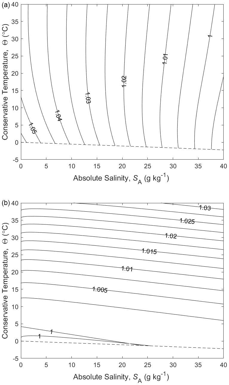
Figure 7 (a) The ratio of the thermal expansion coefficients with respect to Conservative Temperature and potential temperature, ${\stackrel{\mathrm{̃}}{\mathit{\alpha }}}^{\mathit{\theta }}/{\widehat{\mathit{\alpha }}}^{\mathrm{\Theta }}={\stackrel{\mathrm{̃}}{\mathrm{\Theta }}}_{\mathit{\theta }}$. (b) The ratio of the saline contraction coefficients at constant potential temperature to that at constant Conservative Temperature, ${\stackrel{\mathrm{̃}}{\mathit{\beta }}}^{\mathit{\theta }}/{\widehat{\mathit{\beta }}}^{\mathrm{\Theta }}=\mathrm{1}+({\widehat{\mathit{\alpha }}}^{\mathrm{\Theta }}/{\widehat{\mathit{\beta }}}^{\mathrm{\Theta }}){\widehat{\mathit{\theta }}}_{S_{\mathrm{A}}}/{\widehat{\mathit{\theta }}}_{\mathrm{\Theta }}$, at p=0 dbar.

Now we turn our attention to the relative error in the salinity derivative of the equation of state, which, from Eq. (10), can be written approximately as

$$\begin{array}{}\text{(12)}& \left({\stackrel{\mathrm{̃}}{\mathit{\rho }}}_{S_{*}}-{\widehat{\mathit{\rho }}}_{S_{*}}\right)/{\widehat{\mathit{\rho }}}_{S_{*}}={\stackrel{\mathrm{̃}}{\mathit{\beta }}}^{\mathit{\theta }}/{\widehat{\mathit{\beta }}}^{\mathrm{\Theta }}-\mathrm{1},\end{array}$$

and the ratio, ${\stackrel{\mathrm{̃}}{\mathit{\beta }}}^{\mathit{\theta }}/{\widehat{\mathit{\beta }}}^{\mathrm{\Theta }}$, has been plotted (at p=0 dbar) in Fig. 7b. This figure shows that the relative error in the salinity derivative, $({\stackrel{\mathrm{̃}}{\mathit{\rho }}}_{S_{*}}-{\widehat{\mathit{\rho }}}_{S_{*}})/{\widehat{\mathit{\rho }}}_{S_{*}}$, is an increasing (approximately quadratic) function of temperature, being approximately zero at 0 ^∘C, 1 % error at 20 ^∘C, and 2 % error at 30 ^∘C. An alternative derivation of these implications of Eq. (10) is given in Appendix B.

We conclude that under option 2, wherein the temperature variable of an EOS-80-based model (whose polynomial equation of state expects to have potential temperature as its input temperature) is interpreted as being Conservative Temperature, there are persistent errors in the contribution of the isobaric salinity gradient to the isobaric density gradient that are approximately proportional to temperature squared, with the error being approximately 1 % at a temperature of 20 ^∘C (mostly due to the salinity derivative of in situ density at constant potential temperature being 1 % different to the corresponding salinity derivative at constant Conservative Temperature). Larger fractional errors in the contribution of the isobaric temperature gradient to the thermal wind equation do occur (of up to 6 %), but these are restricted to the rather small volume of the ocean that is quite fresh.

In Fig. 8 we have evaluated how much the meridional isobaric density gradient changes in the upper 1000 dbar of the world ocean when the temperature argument in the expression for density is switched from θ to Θ. As explained above, this switch is almost equivalent to the density difference between calling the EOS-80 and the TEOS-10 equations of state using the same numeric inputs for each. We find that 19 % of these data has the isobaric density gradient changed by more than 1 % when switching from θ to Θ. The median value of the percentage error is 0.22 %; that is, 50 % of the data shallower than 1000 dbar has the isobaric density gradient changed by more than 0.22 % when switching from using EOS-80 to TEOS-10, with the same numerical temperature input, which we are interpreting as being Θ.

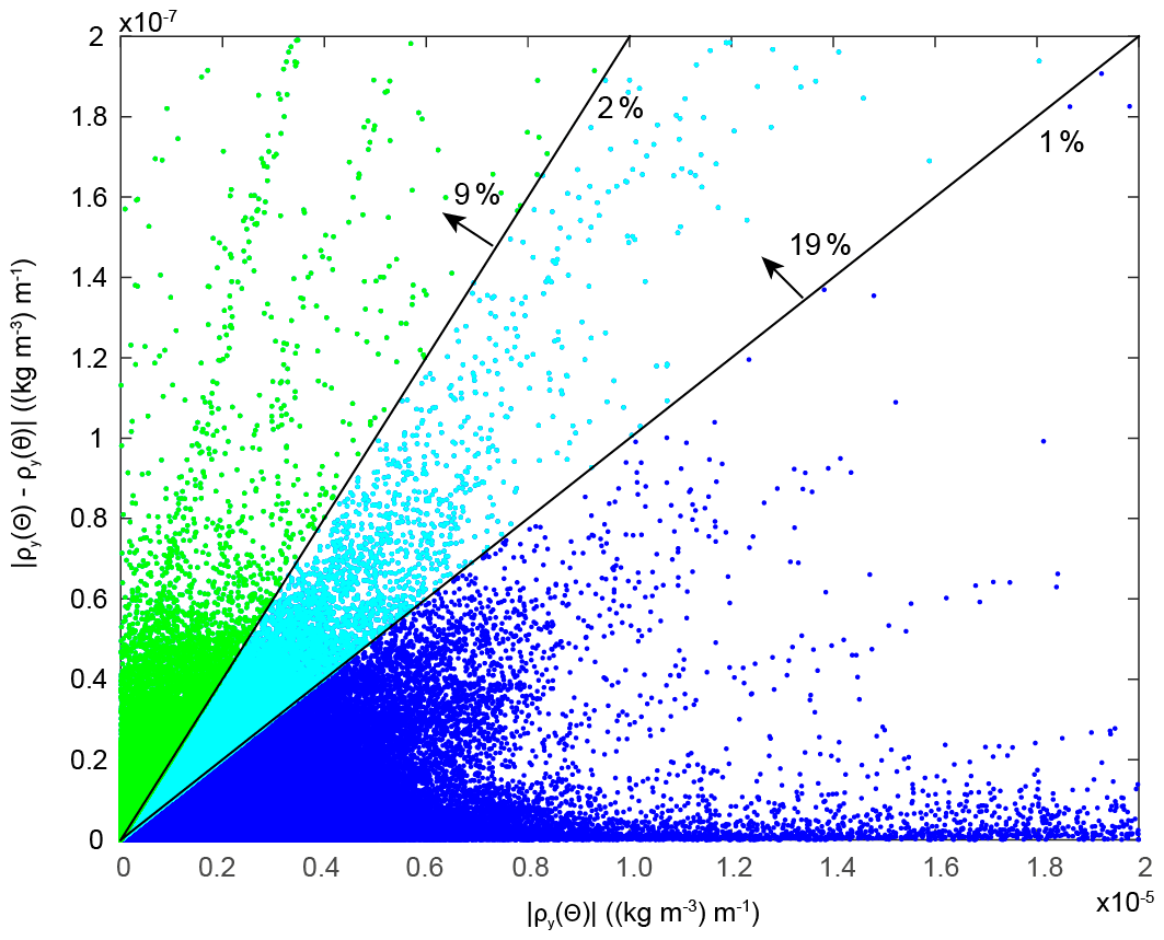
Figure 8 The northward density gradient at constant pressure (the horizontal axis) for data in the global ocean atlas of Gouretski and Koltermann (2004) for p<1000 dbar. The vertical axis is the magnitude of the difference between evaluating the density gradient using Θ versus θ as the temperature argument in the expression for density. This is virtually equivalent to the density difference between calling the EOS-80 and the TEOS-10 equations of state using the same numeric inputs for each. The 1 % and 2 % lines indicate where the isobaric density gradient is in error by 1 % and 2 %. 19 % of the data shallower than 1000 dbar has the isobaric density gradient changed by more than 1 % when switching between the equations of state. The median value of the percentage error in the isobaric density gradient is 0.22 %.

Figure 8 should not be interpreted as being the extra error involved with taking T_model to be Conservative Temperature in EOS-80 ocean models because, due to the lack of interior non-conservative source terms, the interpretation of T_model as being potential temperature is already incorrect by an amount that scales as Θ minus θ. Rather, Fig. 8 illustrates the error in an EOS-80 model due to the use of an equation of state that is not appropriate to the way that its temperature variable is treated in the model.

4.3 Evaluating the options for EOS-80 models

Under option 1 wherein T_model is interpreted as potential temperature, there is a non-conservation of heat at the sea surface, with the ocean seeing one heat flux and the atmosphere immediately above it seeing another, with 5 % of the differences in these heat fluxes being larger than approximately ±100 mW m⁻² and a net imbalance of 16 mW m⁻².

Under option 2 wherein T_model is interpreted as Conservative Temperature, the air–sea flux imbalance does not arise, but two other inaccuracies arise. First, under option 2 the bulk formulae that determine part of the air–sea flux are based on the surface values of Θ rather than of θ (for which the bulk formulae are designed). Second, the isobaric density gradient in the upper ocean is typically different by ∼1 % to the isobaric density gradient that would be found if the TEOS-10 equation of state had been adopted in these models. These two aspects of option 2 are considered less serious than not conserving heat at the sea surface by up to ±100 mW m⁻². Neither of the two inaccuracies that arise under option 2 are fundamental thermodynamic errors. Rather, they are equivalent to the ocean modeller choosing (i) slightly different bulk formulae and (ii) a slightly different equation of state. The constants in the bulk formulae are very poorly known so that the switching from θ to Θ in their use will be well within their uncertainty (Cronin et al., 2019,) while the ∼1 % change to the isobaric density gradient due to using the different equations of state is at the level of our knowledge of the equation of state of seawater (see the discussion section below).

We conclude that option 2 wherein the T_model in EOS-80 models is interpreted as Conservative Temperature is much preferred as it treats the air–sea heat flux in a manner consistent with the first law of thermodynamics, and the treatment of T_model as being a conservative variable in the ocean interior is more consistent with it being Conservative Temperature than being potential temperature. These same two features of ocean models mean that T_model cannot be accurately interpreted as potential temperature, since both the surface flux boundary condition and the lack of the non-conservative source terms in the ocean interior mean that these ocean models continually force T_model away from being potential temperature, even if it was initialized as such.

5 Comparison with ocean observations

Now that we have argued that T_model of EOS-80-based models should be interpreted as being Conservative Temperature, how then should the model-based estimates of ocean heat content and ocean heat flux be compared with ocean observations and ocean atlas data? The answer is by evaluating the ocean heat content correctly in the observed data sets using TEOS-10, whereby the observed data are used to calculate Conservative Temperature, and this is used together with $c_p^{\mathrm{0}}$ to evaluate ocean heat content and meridional heat fluxes.

We have made the case that the salinity variable in CMIP ocean models that have been spun up for several centuries is Preformed Salinity S_* for the TEOS-10-compliant models and is $S_{*}/u_{\mathrm{PS}}$ for the EOS-80-compliant models. Hence, it is the value of either S_* or $S_{*}/u_{\mathrm{PS}}$ calculated from ocean observations to which the model salinities should be compared. Preformed Salinity S_* is different to Reference Salinity S_R by only the ratio $\mathrm{0.26}=\mathrm{0.35}/\mathrm{1.35}$ compared with the difference between Absolute Salinity and Preformed Salinity (see Fig. 4), and these differences are generally only significantly different to zero at depths exceeding 500 m. Note that Preformed Salinity can be evaluated from observations of Practical Salinity using the Gibbs SeaWater (GSW) software gsw_Sstar_from_SP.

6 Discussion and recommendations

We have made the case that it is advisable to avoid non-conservative sources of heat at the sea surface. It is the prior interpretation of the temperature variable in EOS-80-based models as being potential temperature that implies that the ocean receives a heat flux that is larger by ΔQ than the heat that is lost from the atmosphere. Since there are some areas of the ocean surface where ΔQ is as large as the mean rate of global warming, the issue is important in practice. This realization has motivated the new interpretation of the prognostic temperature of EOS-80 ocean models as being Conservative Temperature (our option 2, Sect. 4.2).

A consequence of this new interpretation of the prognostic temperature variable of all CMIP ocean models as being Conservative Temperature means that the EOS-80-based models suffer from a relative error of ∼1 % in their isobaric gradient of in situ density in the warm upper ocean. How worried should we be about this error? One perspective on this question is to simply note (from above) that there are larger relative errors (∼2.7 %) in the thermal wind equation in the deep ocean due to the neglect of variations in the relative composition of sea salt. Another perspective is to ask how well science even knows the thermal expansion coefficient, for example. From Appendices K and O of IOC et al. (2010) (and Sect. 7 of McDougall and Barker, 2011) we see that the root mean square (rms) value of the differences between the individual laboratory-based data points of the thermal expansion coefficient and the thermal expansion coefficient obtained from the fitted TEOS-10 Gibbs function is $\mathrm{0.73}\times {\mathrm{10}}^{-\mathrm{6}}$ K⁻¹, which is approximately 0.5 % of a typical value of the thermal expansion coefficient in the ocean. Without a proper estimation of the number of degrees of freedom represented by the fitted data points, we might estimate the relative error of the thermal expansion coefficient obtained from the fitted TEOS-10 Gibbs function as being half of this, namely 0.25 %. So a typical relative error in the isobaric density gradient of ∼1 % in the upper ocean due to using Θ rather than θ as the temperature input seems undesirable but not serious.

We must also acknowledge that all models have ignored the difference between Preformed Salinity, Reference Salinity, and Absolute Salinity (which is the salinity variable from which density is accurately calculated). As discussed in IOC et al. (2010), Wright et al. (2011), and McDougall and Barker (2011), glossing over these issues of the spatially variable composition of sea salt, which is the same as glossing over the effects of biogeochemistry on salinity and density, means that all our ocean and climate models have errors in their thermal wind (vertical shear of horizontal velocity) that globally exceed 2.7 % for half the ocean volume deeper than 1000 m. In the deep North Pacific Ocean, the misestimation of thermal wind is many times this 2.7 % value. The recommended way of incorporating the spatially varying composition of seawater into ocean models appears as Sect. A20 in the TEOS-10 manual (IOC et al., 2010) and as Sect. 9 in McDougall and Barker (2011), with ocean models needing to carry a second salinity type variable. While it is true that this procedure has the effect of relaxing the model towards the non-standard seawater composition of today's ocean, it is clearly advantageous to make a start with this issue by incorporating the non-conservative source terms that apply to the present ocean rather than to continue to ignore the issue altogether. As explained in these references, once the modelling of ocean biogeochemistry matures, the difference between the various types of salinity can be calculated in real time in an ocean model without the need for referring to historical data.

Nevertheless, we acknowledge that no published ocean model to date has attempted to include the influence of biogeochemistry on salinity and density, and therefore we recommend that the salinity from both observations and model output be treated as Preformed Salinity S_*.

6.1 Contrasts to the recommendations of Griffies et al. (2016)

How does this paper differ from the recommendations in Griffies et al. (2016)? That paper recommended that the ocean heat content and meridional transport of heat should be calculated using the model's temperature variable and the model's value of $c_p^{\mathrm{0}}$, and we strenuously agree. However, in the present paper we argue that the temperature variable carried by an EOS-80-based ocean model should be interpreted as being Conservative Temperature and not be interpreted as being potential temperature. This idea was raised as a possibility in Griffies et al. (2016), but the issue was left unclear in that paper. For example, Sect. D2 of Griffies et al. (2016) recommends that TEOS-10-based models archive potential temperature (as well as their model variable, Conservative Temperature) “in order to allow meaningful comparisons” with the output of the EOS-80-based models. We now disagree with this suggestion; the thesis of the present paper is that the temperature variables of both EOS-80- and TEOS-10-based models are already directly comparable – they should both be interpreted as being Conservative Temperature, and they should both be compared with Conservative Temperature from observations. The fact that the model's temperature variable is labelled “thetao” in EOS-80 models and “bigthetao” in TEOS-10-based models we now see as very likely to cause confusion, since we are recommending that the temperature outputs of both types of ocean models should be interpreted as Conservative Temperature.

The present paper also diverges from Griffies et al. (2016) in the way that the salinity variables in CMIP ocean models should be interpreted and thus compared to observations. Griffies et al. (2016) interpret the salinity variable in TEOS-10-based ocean models as being Reference Salinity S_R, whereas we show that these models actually carry Preformed Salinity S_* but have errors in their calculation of densities. Similarly, Griffies et al. (2016) interpret the salinity variable in EOS-80-based ocean models as being Practical Salinity S_P, whereas we show that these models actually carry $S_{*}/u_{\mathrm{PS}}$: that is, Preformed Salinity divided by the constant, u_PS. This distinction between the present paper and Griffies et al. (2016) is negligible in the upper ocean where Preformed Salinity is almost identical to Reference Salinity (because the composition of seawater in the upper ocean is close to Reference Composition), but in the deeper parts of the ocean, the distinction is not negligible; for example, based on the work of McCarthy et al. (2015) we have shown that the use of Absolute Salinity versus Preformed Salinity leads to ∼1 Sv difference in the meridional overturning stream function in the North Atlantic at a depth of 2700 m. However, in this deeper part of the ocean, even though the difference between Absolute Salinity and Preformed Salinity is not negligible, the difference between Preformed Salinity and Reference Salinity (which the TEOS-10-based ocean models have to date assumed their salinity variable to be) is smaller in the ratio $\mathrm{0.35}/\mathrm{1.35}=\mathrm{0.26}$ (see Fig. 4). That is, if the salinity output of a TEOS-10-based ocean model was taken to be Reference Salinity, the error would be only a quarter of the difference between Absolute Salinity and Preformed Salinity, a difference which limits the accuracy of the isobaric density gradients in the deeper parts of ocean models (see Fig. 4). A similar remark applies to EOS-80-based ocean models if their salinity output is regarded as being Practical Salinity instead of being (as we propose) $S_{*}/u_{\mathrm{PS}}$.

6.2 Summary table of ocean heat content imbalances

In Table 1 we summarize the effects of uncertainties in physical or numerical processes in estimating ocean heat content or its changes. The first two rows are the rate of warming (expressed in m Wm⁻² averaged over the sea surface) due to anthropogenic global warming and due to geothermal heating. The third row is an estimate of the surface heat flux equivalent of the depth-integrated rate of dissipation of turbulent kinetic energy, and the fourth is an estimate of the neglected net flux of potential enthalpy at the sea surface due to the evaporation and precipitation of water occurring at different temperatures.

The next (fifth) row is the consequence of considering the scenario in which all the radiant heat is absorbed into the ocean at a pressure of 25 dbar rather than at the sea surface. The derivative of specific enthalpy with respect to Conservative Temperature at 25 dbar, ${\widehat{h}}_{\mathrm{\Theta }}$, is $c_p^{\mathrm{0}}$ times the ratio of the absolute in situ temperature at 25 dbar, (T₀+t), to the absolute potential temperature, (T₀+θ), at this pressure (see Eq. A11.15 of IOC et al., 2010). The ratio of ${\widehat{h}}_{\mathrm{\Theta }}$ to $c_p^{\mathrm{0}}$ at 25 dbar is typically different to unity by $\mathrm{6}\times {\mathrm{10}}^{-\mathrm{6}}$, and taking a typical rate of radiative heating of 100 W m⁻² over the ocean's surface leads to 0.6 mW m⁻² as the area-averaged rate of misestimation of the surface flux of Conservative Temperature for this assumed pressure of penetrative radiation. Since this is so small, the use of $c_p^{\mathrm{0}}$ (rather than ${\widehat{h}}_{\mathrm{\Theta }}$) to convert the divergence of the radiative heat flux into a flux of Conservative Temperature is well-supported, providing the correct diagnostics are used for the calculation (such diagnostic issues may be responsible for the heat budget closure issues identified by Irving et al., 2021).

The next six rows of Table 1 list the mean and twice the standard deviation of the volume-integrated non-conservative production of Conservative Temperature, potential temperature, and specific entropy (all in mW m⁻²) at the sea surface. The following two rows are the results we have found in this paper for the air–sea heat flux error that is made if the EOS-80 temperature is taken to be potential temperature.

The final three rows show that ocean models, being cast in flux divergence form with heat fluxes being passed between one grid box and the next, do not have appreciable numerical errors in deducing air–sea fluxes from changes in the volume-integrated heat content.

The estimate from Graham and McDougall (2013) of −10 mW m⁻¹ is for the net interior production of θ, so this is a net destruction. A steady state requires this amount of extra flux of θ at the sea surface (so it can be consumed in the interior). Our estimate of this extra flux of θ at the sea surface is 16 mW m⁻², which is only a little larger than the estimate of Graham and McDougall (2013).

6.3 Summary of recommendations

In summary, this paper has argued for the following guidelines for analysing the CMIP model runs. We should interpret the prognostic temperature variable of all CMIP models (whether they are based on the EOS-80 or the TEOS-10 equation of state) as being Conservative Temperature, compare the model's prognostic temperature with the Conservative Temperature, Θ, of observational data, calculate the ocean heat content as the volume integral of the product of (i) in situ density (for non-Boussinesq models or reference density for Boussinesq), (ii) the model's prognostic temperature, Θ, and (iii) the model's value of $c_p^{\mathrm{0}}$, interpret the salinity variable of the model output as being Preformed Salinity S_* for TEOS-10-based ocean models and $S_{*}/u_{\mathrm{PS}}$ for EOS-80-based ocean models (so it is advisable to post-multiply the salinity output of EOS-80 models by u_PS in order to have the salinity outputs of all types of CMIP models as Preformed Salinity S_*), and compare the model's salinity variable with Preformed Salinity, S_*, calculated from ocean observations.

Sea surface temperature should be taken as the model's prognostic temperature in the case of EOS-80 models (since this is the temperature that was used in the bulk formulae), and as the calculated and stored values of potential temperature in the case of TEOS-10 models.

Ensure that all required fixed variables, such as $c_p^{\mathrm{0}}$, (Boussinesq) reference density, seawater volume, and the freezing equation are saved to the CMIP archives alongside the prognostic temperature and salinity variables so that analysts have all components required to accurately interpret the model fields. In addition, providing the full-depth OHC time series for each simulation would provide a quantified target for analysts to compare and contrast changes across models and simulations.

Note that this sixth recommendation for EOS-80-based models exposes an unavoidable inconsistency in that the surface values of the model's prognostic temperature are best regarded internally in the ocean model as being Conservative Temperature, but we cannot avoid the fact that this same temperature was used as the sea surface (in situ) temperature in the bulk formulae during the running of such ocean models. Issues such as these will not arise when all ocean models have been converted to the TEOS-10 equation of state.

How then should the model's salinity and temperature outputs, S_* and Θ, be used to evaluate dynamical concepts such as stream functions and dynamic height? The answer most consistent with the running of a numerical model is to use the equation of state that the model used together with the model's temperature and salinity outputs on the native grid of the model. This method is important when studying detailed dynamical balances in ocean model output. But since we now have the output salinity and temperature of both EOS-80 and TEOS-10 models being the same (namely S_* and Θ), there is an efficiency and simplicity argument to analyse the output of all these models in the same manner using algorithms from the Gibbs SeaWater (GSW) Oceanographic Toolbox of TEOS-10 (McDougall and Barker, 2011). Doing these model intercomparisons often involves interpolating the model outputs to depths (or pressures) different than those used in the original ocean model, therefore incurring some interpolation errors. While the use of the GSW software means that the in situ density will be calculated slightly differently than in some of the forward models, thus affecting the thermal wind and sea level rise, these differences are small, as can be seen by comparing Figs. A5.1 and A5.2 of the TEOS-10 manual (IOC et al., 2010). Hence, we think that it is viable for most purposes to evaluate density and dynamic height using the GSW Oceanographic Toolbox, with the input salinity to this GSW code being the model's Preformed Salinity and the temperature input being the Conservative Temperature, which as we have argued, are the model's prognostic salinity and temperature variables.

Another issue that may arise is when a TEOS-10-based model has been run with Conservative Temperature, but the monthly mean Conservative Temperature output has been converted into potential temperature before sending the model output to the CMIP archive. What is the damage done if this inaccurately averaged value of potential temperature is converted back to Conservative Temperature using only the monthly mean potential temperature and salinity? While such an issue is perhaps an operational detail that takes us some distance from our intention of writing an academic paper about these issues, nevertheless we show Fig. 9, which indicates that transforming between these monthly averaged values is not a serious issue for relatively coarse-resolution ocean models.

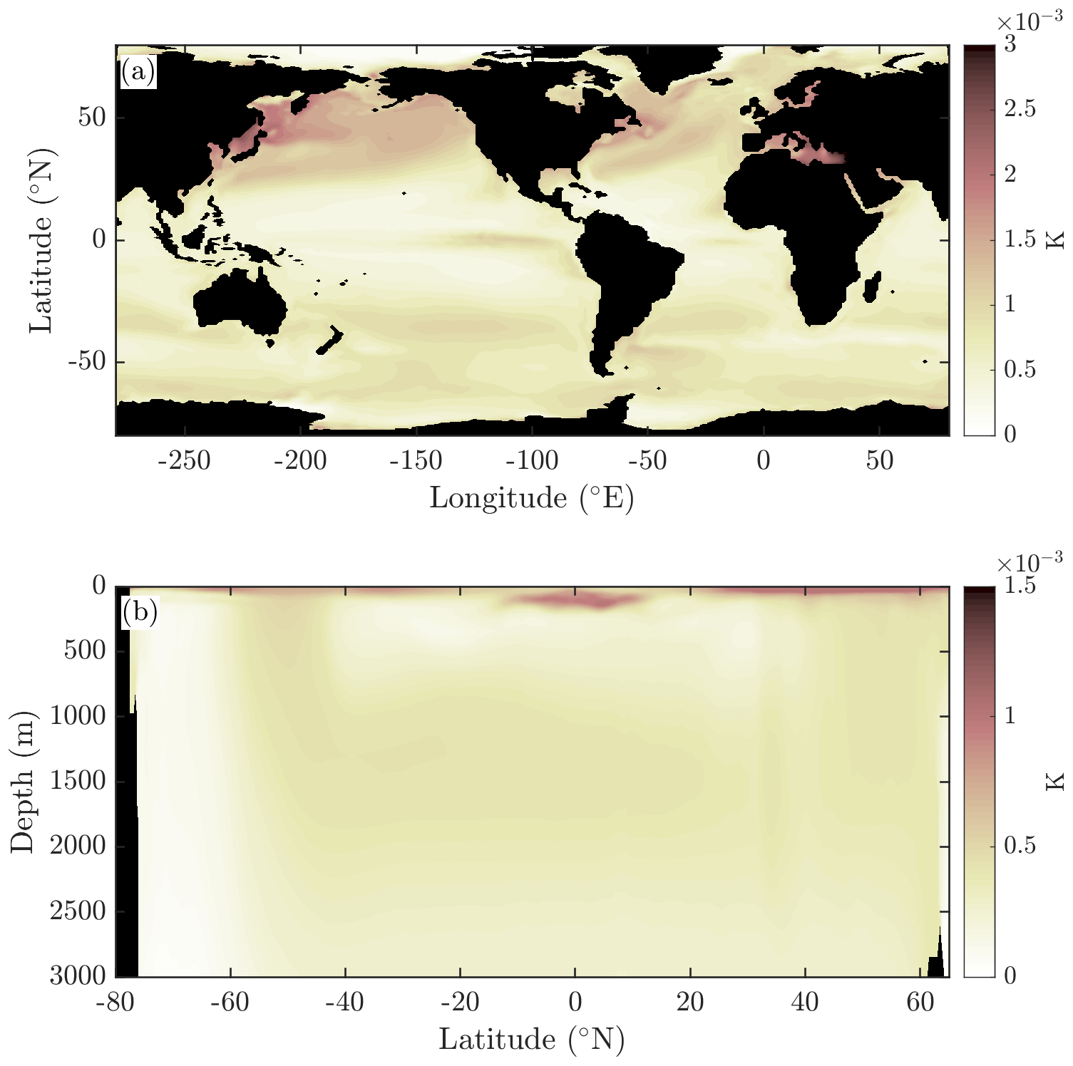
Figure 9 The RMSE (K) in evaluating Conservative Temperature from the CMIP6 archived monthly averaged values of potential temperature and salinity compared with averaging the instantaneous values of Conservative Temperature for a month at the (a) surface and (b) the zonal mean. These quantities are calculated from 50 years of temporally averaged output from the ACCESS-CM2 model's pre-industrial control simulation. The errors are seen to be no larger than a few millikelvin (mK).

Appendix A: A non-seawater thermodynamic interpretation of option 1

Ocean models have always assumed a constant isobaric heat capacity and have traditionally assumed that the model's temperature variable is whatever temperature the equation of state was designed to accept. Here we enquire whether there is a way of justifying option 1 thermodynamically in the sense that option 1 would be totally consistent with thermodynamic principles for a fluid that is different to real seawater.

That is, we pursue the idea that these EOS-80-based ocean models are not actually models of seawater but are models of a slightly different fluid. We require a fluid that is identical to seawater in some respects, such as having the same dissolved material (Millero et al., 2008) and the same issues around Absolute Salinity, Preformed Salinity, and Practical Salinity, as well as the same in situ density as real seawater (at given values of Absolute Salinity, potential temperature, and pressure). But we require the expression for the enthalpy of this new fluid to be different to that of real seawater.

The difference that we envisage between real seawater and this new fluid is that, at zero pressure, the enthalpy of the new fluid is given exactly by the constant value $c_p^{\mathrm{0}}$ times potential temperature θ. That is, for the new fluid, potential enthalpy h⁰ is simply $c_p^{\mathrm{0}}\mathit{\theta }$ (as it would be for an ideal gas), and the air–sea interaction for this new fluid would be exactly as it occurs in the EOS-80-based models. Moreover, conservation of potential temperature is justified for this new fluid, and the density and thermal wind would also be correctly evaluated in these EOS-80-based models.

The enthalpy of this new fluid is then given by (since h_P=v)

$$\begin{array}{}\text{(A1)}& \stackrel{\mathrm{˘}}{h}\left(S_{\mathrm{A}},\mathit{\theta },p\right)=c_p^{\mathrm{0}}\mathit{\theta }+\underset{P_{\mathrm{0}}}{\overset{P}{\int }}\stackrel{\mathrm{̃}}{v}\left(S_{\mathrm{A}},\mathit{\theta },p^{\prime }\right)d{P}^{\prime },\end{array}$$

while the entropy of this new fluid needs to obey the consistency relationship, ${\stackrel{\mathrm{˘}}{\mathit{\eta }}}_{\mathit{\theta }}={\stackrel{\mathrm{˘}}{h}}_{\mathit{\theta }}(p=\mathrm{0})/(T_{\mathrm{0}}+\mathit{\theta })$, which reduces to

$$\begin{array}{}\text{(A2)}& {\stackrel{\mathrm{˘}}{\mathit{\eta }}}_{\mathit{\theta }}={\displaystyle \frac{c_p^{\mathrm{0}}}{\left(T_{\mathrm{0}}+\mathit{\theta }\right)}},\end{array}$$

where T₀=273.15 K is the Celsius zero point. This consistency relationship is derived directly from the fundamental thermodynamic relationship (see Table P1 of IOC et al., 2010). Integrating Eq. (A2) with respect to potential temperature at constant salinity leads to the following expression for entropy that our new fluid must obey:

$$\begin{array}{}\text{(A3)}& \stackrel{\mathrm{˘}}{\mathit{\eta }}\left(S_{\mathrm{A}},\mathit{\theta }\right)=c_p^{\mathrm{0}}\ln \left(\mathrm{1}+{\displaystyle \frac{\mathit{\theta }}{T_{\mathrm{0}}}}\right)+a\left({\displaystyle \frac{S_{\mathrm{A}}}{S_{\mathrm{SO}}}}\right)\ln \left({\displaystyle \frac{S_{\mathrm{A}}}{S_{\mathrm{SO}}}}\right).\end{array}$$

The variation here with salinity is taken from the TEOS-10 Gibbs-function-derived expression for specific entropy, which contains the last term in Eq. (A3) with the coefficient a being $a=-\mathrm{9.310292413479596}$ J kg⁻¹ K⁻¹ (this is the value of the coefficient derived from the g₁₁₀ coefficient of the Gibbs function – Appendix H of IOC et al., 2010 – allowing for our version of the normalization of salinity, $S_{\mathrm{A}}/S_{\mathrm{SO}}$). This term was derived by Feistel (2008) to be theoretically correct at vanishingly small Absolute Salinities.

With these definitions (Eqs. A1 and A3) of enthalpy and entropy of our new fluid, we have completely defined all the thermophysical properties of the fluid (see Appendix P of IOC et al., 2010, for a discussion). Many aspects of the fluid are different to seawater, including the adiabatic lapse rate (and hence the relationship between in situ and potential temperatures), since the adiabatic lapse rate is given by $\mathrm{\Gamma }={\stackrel{\mathrm{˘}}{h}}_{\mathit{\theta }P}/{\stackrel{\mathrm{˘}}{\mathit{\eta }}}_{\mathit{\theta }}$, and while the numerator is the same as for seawater (since ${\stackrel{\mathrm{˘}}{h}}_{\mathit{\theta }P}={\stackrel{\mathrm{̃}}{h}}_{\mathit{\theta }P}={\stackrel{\mathrm{̃}}{v}}_{\mathit{\theta }}$), the denominator, ${\stackrel{\mathrm{˘}}{\mathit{\eta }}}_{\mathit{\theta }}$, which is now given by Eq. (A2), can be up to 6 % different to the corresponding function, ${\stackrel{\mathrm{̃}}{\mathit{\eta }}}_{\mathit{\theta }}$, appropriate to real seawater.

We conclude that this is indeed a conceptual way of forcing the EOS-80-based models to be consistent with thermodynamic principles. That is, we have shown that these EOS-80 models are not models of seawater, but they do accurately model a different fluid whose thermodynamic definition we have given in Eqs. (A1) and (A3). This new fluid interacts with the atmosphere in the way that EOS-80 models have assumed to date; the potential temperature of this new fluid is correctly mixed in the ocean in a conservative fashion, and the equation of state is written in terms of the model's temperature variable, namely potential temperature.

Hence, we have constructed a fluid which is thermodynamically different to seawater, but it does behave exactly as these EOS-80 models treat their model seawater. That is, we have constructed a new fluid for which, if seawater had these thermodynamic characteristics, the EOS-80 ocean models would have correct thermodynamics while being able to interpret the model's temperature variable as potential temperature.

But this does not change the fact that in order to make these EOS-80 models thermodynamically consistent in this way we have ignored the real variation at the sea surface of the isobaric specific heat capacity – a variation that we know can be as large as 6 %.

Hence, we do not propose this non-seawater explanation as a useful rationalization of the behaviour of EOS-80-based ocean models. Rather, it seems less dramatic and more climatically relevant to adopt the simpler interpretation of option 2. Under this option we accept that the model is modelling actual seawater, that the model's temperature variable is in fact Conservative Temperature, and that there are some errors in the equation of state of these EOS-80 models that amount to errors of the order of 1 % in the thermal wind relation throughout much of the upper (warm) ocean. That is, so long as we interpret the temperature variable of these EOS-80-based models as Conservative Temperature, they are fine except that they have used an incorrect equation of state; they have used $\stackrel{\mathrm{̃}}{\mathit{\rho }}$ rather than $\widehat{\mathit{\rho }}$. Apart from this “error” in the ocean code, option 2 is a consistent interpretation of the ocean model thermodynamics and dynamics. In ocean models there are always questions of how to parameterize ocean mixing. To this uncertain aspect of ocean physics, under option 2 we add the less than desirable expression that is used to evaluate density in EOS-80-based ocean models in CMIP.

Appendix B: An alternative derivation of Eq. (10)

Equation (10) is an expression for the error in the isobaric density gradient when Conservative Temperature is used as the input temperature variable to the EOS-80 equation of state (which expects its input temperature to be potential temperature). An alternative accurate expression to Eq. (9) for the isobaric density gradient is

$$\begin{array}{}\text{(B1)}& {\stackrel{\mathrm{̃}}{\mathit{\rho }}}_{S_{*}}{\mathrm{\nabla }}_P{S}_{*}+{\stackrel{\mathrm{̃}}{\mathit{\rho }}}_{\mathit{\theta }}{\mathrm{\nabla }}_P\mathit{\theta },\end{array}$$

and subtracting this from the incorrect expression (Eq. 8) gives the following expression for the model's error in evaluating the isobaric gradient of in situ density:

$$\begin{array}{}\text{(B2)}& \mathrm{error}\mathrm{in}{\mathrm{\nabla }}_P\mathit{\rho }={\stackrel{\mathrm{̃}}{\mathit{\rho }}}_{\mathit{\theta }}{\mathrm{\nabla }}_P(\mathrm{\Theta }-\mathit{\theta }).\end{array}$$

An approximate fit to the temperature difference, Θ−θ, as displayed in Fig. 2 is

$$\begin{array}{}\text{(B3)}& (\mathrm{\Theta }-\mathit{\theta })\approx \mathrm{0.05}\mathrm{\Theta }\left(\mathrm{1}-{\displaystyle \frac{S_{\mathrm{A}}}{S_{\mathrm{SO}}}}\right)-\mathrm{1.75}\times {\mathrm{10}}^{-\mathrm{3}}\mathrm{\Theta }\left(\mathrm{1}-{\displaystyle \frac{\mathrm{\Theta }}{\mathrm{25}{}^{\circ }\mathrm{C}}}\right),\end{array}$$

and using this approximate expression in the right-hand side of Eq. (B2) gives

$$\begin{array}{}\text{(B4)}& \begin{array}{rl}{\displaystyle \frac{\mathrm{error}\mathrm{in}{\mathrm{\nabla }}_P\mathit{\rho }}{{\stackrel{\mathrm{̃}}{\mathit{\rho }}}_{\mathit{\theta }}}}\approx & \left[\mathrm{0.05}\left(\mathrm{1}-{\displaystyle \frac{S_{*}}{S_{\mathrm{SO}}}}\right)-\mathrm{1.75}\times {\mathrm{10}}^{-\mathrm{3}}\right.\\ & \left.\left(\mathrm{1}-{\displaystyle \frac{\mathrm{\Theta }}{\mathrm{12.5}{}^{\circ }\mathrm{C}}}\right)\right]{\mathrm{\nabla }}_P\mathrm{\Theta }-{\displaystyle \frac{\mathrm{0.05}}{S_{\mathrm{SO}}}}\mathrm{\Theta }{\mathrm{\nabla }}_P{S}_{*}.\end{array}\end{array}$$

The first part of this expression that multiplies ∇_PΘ corresponds to the proportional error in the thermal expansion coefficient displayed in Fig. 7a. The second part of Eq. (B4) amounts to an error in the saline derivative of the equation of state, with the proportional error (corresponding to Eq. 12) being $-\mathrm{0.05}{\stackrel{\mathrm{̃}}{\mathit{\rho }}}_{\mathit{\theta }}\mathrm{\Theta }/\left({\widehat{\mathit{\rho }}}_{S_{\mathrm{A}}}{S}_{\mathrm{SO}}\right)$, and this is close to the error that can be seen in Fig. 7b. This error is approximately a quadratic function of temperature since the thermal expansion coefficient ${\stackrel{\mathrm{̃}}{\mathit{\rho }}}_{\mathit{\theta }}$ is approximately a linear function of temperature.