Modelling of faults in LoopStructural 1.0

Without properly accounting for both fault kinematics and observations of a faulted surface, it is challenging to create 3D geological models of faulted geological units. Geometries where multiple faults interact, where the faulted surface geometry significantly deviate from a flat plane and where the geological interfaces are poorly characterised by sparse datasets are particular challenges. There are two existing approaches for incorporating faults into geological surface modelling. One approach incorporates the fault displacement into the surface description but does not incorporate fault kinematics and in most cases will produce geologically unexpected results such as shrinking intrusions, fold hinges without offset and layer thickness growth in flat oblique faults. The second approach builds a continuous surface without faulting and then applies a kinematic fault operator to the continuous surface to create the displacement. Both approaches have their strengths; however, neither approach can capture the interaction of faults within complicated fault networks, e.g. fault duplexes, flower structures and listric faults because they either (1) impose an incorrect (not defined by data) fault slip direction or (2) require an over-sampled dataset that describes the faulted surface location. In this study, we integrate the fault kinematics into the implicit surface, by using the fault kinematics to restore observations, and the model domain prior to interpolating the faulted surface. This new approach can build models that are consistent with observations of the faulted surface and fault kinematics. Integrating fault kinematics directly into the implicit surface description allows for complexly faulted stratigraphy and fault–fault interactions to be modelled. Our approach shows significant improvement in capturing faulted surface geometries, especially where the intersection angle between the faulted surface and the fault surface varies (e.g. intrusions, fold series) and when modelling interacting faults (fault duplex).

1 Introduction

Building 3D geological models of complex geometries (e.g. fault duplexes, flower structures, folds, fold interference patterns) from field observations only is still a challenge for most 3D modelling approaches. This challenge exists because many of the observations and structural geology rules are not directly integrated into the mathematical description of the geological models. Structural geologists typically use their knowledge and expertise to formulate a working hypothesis in a digital format, which often derives from a biased conceptual mental picture (Jessell et al., 2014). The modelled geometries will always converge towards the geologist's bias and conceptual model, meaning that model building cannot be used to test different geological hypotheses. An alternative would be to have structural geology concepts encoded in the modelling process. This would enable testing of different geological settings, and the geologists' expertise would be used to assess the viability of these different geometries. This strategy has been developed for modelling folded geometries, based on the structural observations and concepts (Laurent et al., 2016; Grose et al., 2017, 2018, 2019), a mathematical description of the fold geometry that combines a fold structural frame and fold shape profiles. The fold modelling framework has been applied to complex synthetic examples (Laurent et al., 2016; Grose et al., 2017, 2018) and to natural fold examples (Grose et al., 2017, 2019). In this contribution, we adapt the fault frame and a kinematic parameterisation of fault geometries (Jessell and Valenta, 1996; Godefroy et al., 2018; Laurent et al., 2013) and apply it directly to the implicit description of the faulted surfaces. Rather than applying the fault kinematics to the modelled surfaces, we restore the observations and model domain and interpolate the surfaces without the faults.

Defining the geometry of faults and fault networks is a significant component of understanding and characterising the structural architecture of geological terranes. Geometrical descriptions of fault networks and stratigraphic interfaces are used to refine and improve resource characterisation (Cox et al., 1991; Mueller et al., 1988; Vollgger et al., 2015), geophysical inversions (Blaikie et al., 2014) and for understanding complex geological structures (Putz et al., 2006). Implicit 3D geological modelling methods do not directly incorporate fault kinematics into the surface description and as a result cannot reliably model the interaction between faults in fault networks, i.e. duplex faults, flower structures, relay ramps and listric faults (Cherpeau and Caumon, 2015; Calcagno et al., 2008; de la Varga and Wellmann, 2016). It is challenging to build models that are consistent with both geological observations and fault kinematics because the existing methods require the user to choose whether to use observations of the faulted surface or honour fault kinematic observations and knowledge (Laurent et al., 2013; Godefroy et al., 2018).

Modelling the location of the fault surface is generally approached in a manner analogous to modelling bedding or any other structural feature (Calcagno et al., 2008). The challenge for modelling faults is in characterising how the fault interacts with other structural features, e.g. how stratigraphy or other geological features are offset and deformed by the fault. Conceptually there are two approaches for modelling faults: (1) incorporating the fault displacement geometries into the description of the geological surfaces or (2) applying fault displacements after interpolating a continuous surface.

To incorporate faults into the description of the geological surface a step function can be added to the implicit function (Calcagno et al., 2008; de la Varga and Wellmann, 2016; Marechal, 1984). The step function applies a jump in the scalar field value across the fault discontinuity; however, unless (1) the angle between the fault surface and the faulted surface is constant and the angle between the faulted surface and the fault slip direction is constant, the modelled fault is not representative of the true fault movement. There is no direct method of incorporating fault kinematics (movement direction and displacement magnitude) into the description of the geological surface using step functions. One approach that has been used for incorporating fault displacements is to generate multiple model realisations, framing the geological modelling problem as a Bayesian inverse problem. In this probabilistic framework, model data points become parameters for the forward model and fault displacement can be incorporated by including a likelihood function where the fault displacement is expected to come from a prior probability distribution, which may be guided by observations of the fault displacement (de la Varga and Wellmann, 2016; Wellmann et al., 2017; Godefroy et al., 2018). However, this approach is still limited by the inability for fault kinematics to be incorporated into the step function.

The alternative approach is to apply the fault displacement to an already interpolated surface. A first possibility is to apply restoration of the geometric structures surrounding the faults and find the displacement field based on some mechanical likelihood criterion (Thibaut et al., 1996; Maerten and Maerten, 2015). However, finding an objective mechanical criterion is difficult and computationally challenging; an alternative is to construct the geometry of the continuous surface prior to faulting and then to apply the fault operator to the faulted surface (Godefroy et al., 2018; Laurent et al., 2013; Georgsen et al., 2012). In this approach, both the slip direction and the magnitude are used to constrain the fault displacement. Since a continuous surface needs to be interpolated prior to applying the fault, the surface observations within the fault ellipsoid are discarded when interpolating the initial surface. The observations within the fault ellipsoid can then be used to determine the fault displacement magnitude by minimising the misfit between the surface and observations.

Using step functions in the implicit surface description and adding faults to existing surfaces are both useful in basin settings where the pre-fault geometry is reasonably simple and most geometrical complexities are associated with the fault geometry. However, it is unclear how these approaches can be applied to fault networks with a large number of interconnected discrete faults or when modelling complex poly-deformed geometries. When modelling multiple interconnected faults (e.g. splay faults, cross-cutting faults and abutting faults), it can be challenging to properly account for the relative kinematics between faults, especially where the observations of the faulted surfaces are limited to a map view.

In this contribution, we adapt the approach presented by Laurent et al. (2013) and Godefroy et al. (2018), by incorporating the fault operator directly into the implicit function. This uses the fault kinematics to restore the model domain and data points to a pre-fault geometry. The restoration function is defined within a structural frame (Grose et al., 2021a) where the coordinates define fault surface, fault slip direction and the fault extent. This restoration function allows for the kinematics of the fault to be directly incorporated into the modelling workflow. Faults are modelled starting with the most recent and the kinematics are added to every consecutive geological feature added to the model. This application of time-aware geological modelling follows on from previous work for modelling folds (Grose et al., 2017; Laurent et al., 2016). In this paper, we outline the framework for integrating faults in LoopStructural (Grose et al., 2021a). We show case studies ranging in complexity from a simple faulted intrusion, where we demonstrate the limitation of step functions, to a thrust duplex system, and to a faulted fold series using the fold modelling framework from Laurent et al. (2016) and Grose et al. (2017).

2 Background 3D modelling methods

2.1 Surface representation

Three-dimensional structural geological models are a representation of subsurface geology where the geological units are either represented using boundary surfaces (upper and lower contacts) (Wellmann and Caumon, 2018) or a discretisation on a predefined support. There are two approaches that are commonly used for representing surfaces in 3D geological models. The first approach uses explicit surface representation: the geometry of surfaces are contained using a support that is collocated with the surface geometry. The surfaces are represented using discrete objects such as triangulated surfaces, two-dimensional grids or parametric surfaces. The surface geometry is usually built by either directly triangulating data points or using interpolation algorithms to create a smooth surface fitting the data (Chilès, 1999; de Kemp, 1999; Mallet, 1992). The explicit surface representation means that the geometry of the surface is only represented where the surface is located.

The second approach, implicit surface representation, uses isovalues of one or several scalar fields in 3D space to represent the geometry of geological surfaces (e.g. stratigraphic horizons and fault surfaces) (Jessell, 1981; Calcagno et al., 2008; Caumon et al., 2013; Cowan et al., 2003; Frank et al., 2007; Hillier et al., 2014; Lajaunie et al., 1997; Mallet, 2002, 2014; Maxelon et al., 2009; Moyen et al., 2004; Yang et al., 2019; Renaudeau et al., 2019; Manchuk and Deutsch, 2019; Gonçalves et al., 2017; de la Varga et al., 2019). The value of the scalar field represents the distance away from a reference horizon. Alternatively, if the geological interfaces are conformable, the surfaces can be represented by isovalues of the scalar field representing the relative thicknesses between the interfaces. The gradient of the scalar field is a representation of the orientation of the surface being modelled. These scalar fields can be constructed using a variety of different interpolation methods, e.g. co-kriging (Calcagno et al., 2008; de la Varga et al., 2019; Gonçalves et al., 2017; Lajaunie et al., 1997), radial basis functions (Cowan et al., 2003; Hillier et al., 2014) or using discrete interpolation on a predefined support (Irakarama et al., 2020; Caumon et al., 2013; Frank et al., 2007; Moyen et al., 2004; Mallet, 1992). Most modelling approaches use the same interpolation algorithms for all types of geological surfaces even though the physical properties and expected geometries can vary.

These interpolation methods mean models can be created with less bias and are more reproducible. Implicit methods also make it possible to generate a set of model realisations reflecting geological uncertainty (Manchuk and Deutsch, 2019; Cherpeau et al., 2010; Henrion et al., 2010; Wellmann et al., 2010; Lindsay et al., 2012; Yang et al., 2019).

2.2 Faults in implicit modelling

There are a number of existing techniques available for incorporating faults into the implicit approach with methods allowing for topology (Calcagno et al., 2008; Moyen et al., 2004), kinematics (Laurent et al., 2013; Godefroy et al., 2018) and uncertainty (Cherpeau and Caumon, 2015; Cherpeau et al., 2012) to be incorporated into the modelling workflow. Incorporating faults into implicit surface representation is difficult because faults represent a discontinuity in the geological feature being modelled and require a discontinuity in the implicit function. The geometry of the faulted geological feature (stratigraphic interfaces, faults or foliations) should be consistent with the kinematics of the fault.

There are three possible approaches (shown in Fig. 1) that can be used to incorporate faults into implicit surface description: (1) interpolate fault domains using independent implicit functions, (2) incorporate the fault into the domain discretisation or (3) apply a fault operator to a surface already interpolated.

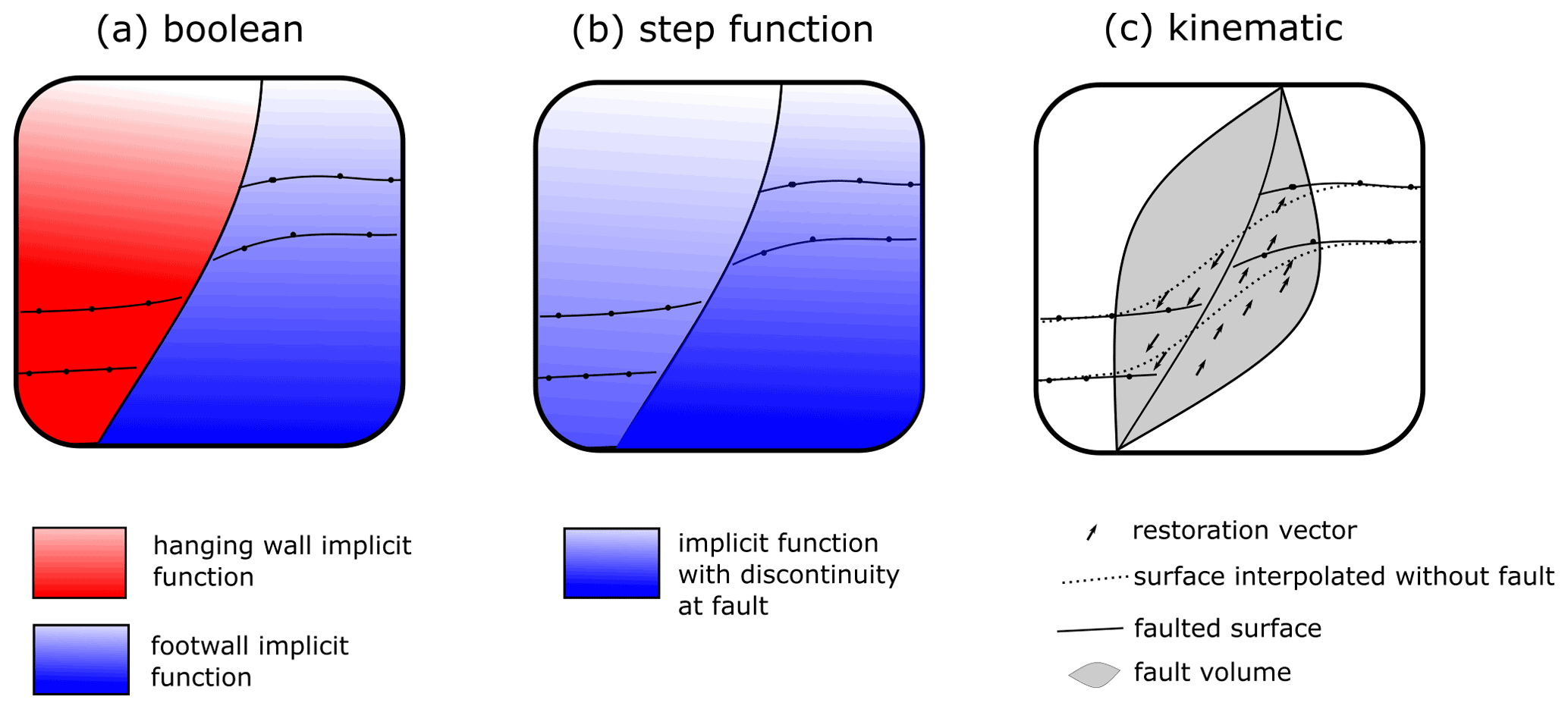
Figure 1 Schematic diagram showing the different approaches for integrating faults into implicit models. (a) The hanging wall and footwall of the fault are represented by two implicit functions (red and blue) where a Boolean operation defined by the fault geometry defines which function is used to represent the geometry. (b) The fault is integrated using a step function in the implicit function where the fault geometry defines the location of the discontinuity. (c) The faulted surface is interpolated without the fault and then restored using the kinematic operator defined by the fault geometry.

The first approach separates the faulted feature using two implicit functions, one on the hanging wall and another on the footwall (Fig. 1a). A Boolean operation using the fault surface geometry is used to define which implicit function (red or blue in Fig. 1a) is used to represent the faulted feature (Caumon et al., 2013; Cowan et al., 2003; Frank et al., 2007).

When the hanging wall and footwall are represented using separate implicit functions, the displacement of the fault is not explicitly defined and will be a result of the observations of the faulted feature. There is no incorporation of the fault kinematics unless these are captured by the location and geometry of observations of the faulted surface. Using different implicit functions for the hanging wall and footwall is suitable for areas where the faults cut across the whole model and there is significant displacement and no continuity expected across the model. For these approaches to work there needs to be a significant amount of data near the fault damage zone to correctly characterise the fault-related deformation, otherwise the kinematic indicators of the layers may not fit the geologist's knowledge about the fault.

The second approach directly incorporates the location of the fault as a discontinuity into a single implicit function (Fig. 1b). This can be done using the polynomial trend of the implicit function using a discontinuous step function (Calcagno et al., 2008; de la Varga et al., 2019; Marechal, 1984). The fault displacement magnitude is not used as an observation for building the model but is found by solving the interpolation system for the co-kriging matrix. In de la Varga and Wellmann (2016), Bayesian inference was applied to incorporate the fault displacement into the implicit modelling workflow by using the observations as parameters for the inverse problem. In their approach, models with different displacements are generated by perturbing the observations of the faulted surface. The objective function that is incorporated into their Bayesian model as a likelihood only considers the magnitude of the displacement and not the direction of displacement. This approach provides an interesting idea of using Bayesian inference as a method for optimising the model parameters in order to try and generate models which fit both geological knowledge and geological observations. An alternative to this approach for discrete implicit methods is to introduce a discontinuity in the regularisation term, by either cutting the interpolation support by the fault geometry (Caumon et al., 2013; Frank et al., 2007) or introducing ghost nodes into the discrete elements (Irakarama et al., 2020).

The third approach (Fig. 1c) integrates the fault kinematics into implicit 3D modelling workflows by using a numerical operator that defines the distribution of fault slip on and close to the fault surface (Godefroy et al., 2017, 2018; Laurent et al., 2013). In these approaches a fault operator models fault displacement within an ellipsoidal fault volume (defined by the grey volume in Fig. 1c). The displacement is discontinuous across the fault surface and decreases smoothly away from the fault. In this approach, a fault volume is defined where the fault displacement is non-zero. The geological interfaces are defined by first interpolating a continuous surface across the fault (dotted line in Fig. 1c). The fault is applied to the surface by displacing the surface by a slip vector scaled by the fault displacement magnitude (shown by the vectors in Fig. 1c). The magnitude of the displacement can be defined within the fault volume either manually or using numerical optimisation techniques (Godefroy et al., 2018). This kinematic approach applies the fault to a surface and is not integrated with the implicit function, meaning it would not directly integrate with approaches where the implicit function represents continuous features such as foliations, conformable stratigraphy or grade shells.

Alternative kinematic models for describing fault displacements exist such as the trishear model (Erslev, 1991; Allmendinger, 1998). Trishear is a kinematic model describing the geometry of fault propagation folds and has been presented in pseudo 3D (Cristallini and Allmendinger, 2001) and in true 3D (Cardozo, 2008). Trishear has been used to understand the structural evolution that has resulted in the geometries observed in the field and as part of seismic interpretations. In the interpretation of reflection seismic data, kinematic fault restoration approaches based on vector fields have been proposed (Hale, 2013; Wu et al., 2015). For example, Wu et al. (2015) determine the fault tip by seismic image processing, then interpolate fault shifts in the volume by least-squares smoothing. However, this model is most directly applicable in contexts where observations are sparse, and the smoothing assumes that fault shifts depend on the stratigraphic orientation. It also restores all faults at once, whereas sequential restorations allow for the fault topology to be included.

2.3 Limitations of the presented approaches

None of the presented approaches are capable of incorporating both fault kinematics and geological observations into the geological surface description. The step function approach is appealing because the fault is incorporated into the model description; however, it cannot capture the kinematics of the fault where the angle of intersection between the fault and faulted surface is variable (e.g. fold series, or intrusions). For example, in Fig. 2a and c a fold series and intrusion are faulted by a reverse fault. In both of these examples the intersection angle between the fault surface and the geometry of the faulted surfaces varies significantly within the model. In Fig. 2b and d the same structures are shown where the fault is incorporated using step functions. Both examples show an increase in the value of the scalar field across the fault geometry; however, the gradient of the implicit function is continuous across the fault. This results in faulted surfaces that do not show the expected kinematics; for example the fold axial traces are not displaced by the fault and the volume of the intrusion shrinks across the fault.

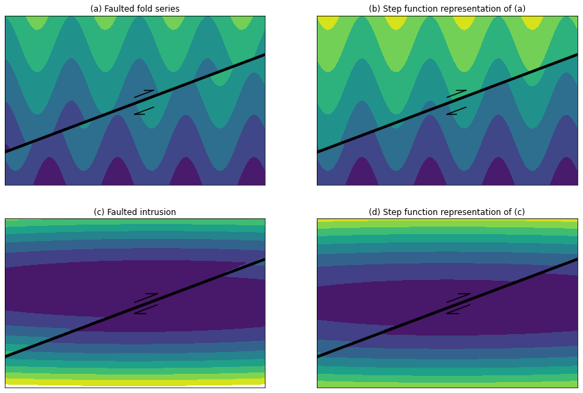
Figure 2 Comparison of true fault kinematics and step function results. (a) A fold series that has been faulted by a reverse fault, where the fold hinges are offset. Panel (b) shows the same fold series as (a) when modelled using a step function where the scalar field on the hanging wall is increased resulting in no displacement of the fold hinges. Panel (c) is a faulted intrusion where the volume is not affected by the fault. Panel (d) shows the same intrusion modelled with a step function where the intrusion shrinks on the hanging wall, resulting in a lower volume intrusion.

3 A kinematic framework for modelling faults

Faults are described by geologists by the movement of rock packages and not only by the location of the discontinuity. Structural geologists describe faults with the fault slip and the displacement magnitude. In a lot of cases, measuring the fault slip direction is impossible, and the geologist will have a conceptual model to describe the fault displacement direction, for example using their conceptual model based on geological knowledge. This means that to properly capture the displacement kinematics in structural models the additional kinematic constraints need to be encoded into the modelling algorithms.

In this contribution, the workflows presented by Laurent et al. (2013) and Godefroy et al. (2018) are modified by incorporating the fault operator into the implicit representation of the geological feature in the model (Fig. 3). The faulted stratigraphy can then be interpolated as a continuous layer where the data points are restored using the fault kinematics. The fault kinematics are integrated into the implicit surface description, meaning that the scalar field, when evaluated in the model domain, captures the fault kinematics.

Figure 3 Schematic diagram showing proposed workflow to integrate fault kinematics to implicit modelling. (a) Observations of reverse fault. (b) Fault frame with restoration vectors showing. (c) Observations and model domain are restored for interpolation; the mesh where interpolation occurs is not deformed and is built in the restored space. (d) Final model is evaluated by applying fault restoration kinematics and evaluating scalar field from mesh in (c).

Integrating the fault kinematics into the implicit modelling system is achieved by

1. building the fault frame, a curvilinear coordinate system representing the fault geometry,

2. defining the fault displacement within the model domain and

3. adding the fault kinematics to the implicit surface description.

3.1 Fault frame

A curvilinear coordinate system (the fault frame, described empirically for natural faults by Walsh and Watterson, 1987) represents different geometrical elements of the fault geometry and is built by interpolating structural observations. The first coordinate (f₀) represents the distance to the fault surface, and the isovalue of 0 will represent the fault surface and can be interpolated from any structural observations of the fault surface, e.g. strike and dip controls and observations of the fault surface location (Fig. 4a). The second coordinate (f₁) measures the displacement direction of the fault, and the normal to the gradient of this field will be parallel to any kinematic indicators for the fault (e.g. slickensides, stretching lineations) and parallel to the fault surface. The third coordinate (f₂) measures the distance in the direction of the fault extent (green line in Fig. 4b), and the gradient of this field will be orthogonal to the gradient norm of the fault surface (f₀) and also orthogonal to the fault displacement field (f₁).

Three local direction vectors are implicitly defined by the normalised gradient of the fault frame for any location:

$$\begin{array}{}\text{(1)}& \begin{array}{rl}& {\mathit{f}}_{\mathrm{0}}=\mathrm{\nabla }{f}_{\mathrm{0}}/\left|\right|f_{\mathrm{0}}\left|\right|,\\ & {\mathit{f}}_{\mathrm{1}}=\mathrm{\nabla }{f}_{\mathrm{1}}/\left|\right|f_{\mathrm{1}}\left|\right|,\\ & {\mathit{f}}_{\mathrm{2}}=\mathrm{\nabla }{f}_{\mathrm{2}}/\left|\right|f_{\mathrm{2}}\left|\right|.\end{array}\end{array}$$

The fault frame can then be queried for any location within the model returning the distance to the fault centre and the fault frame vectors.

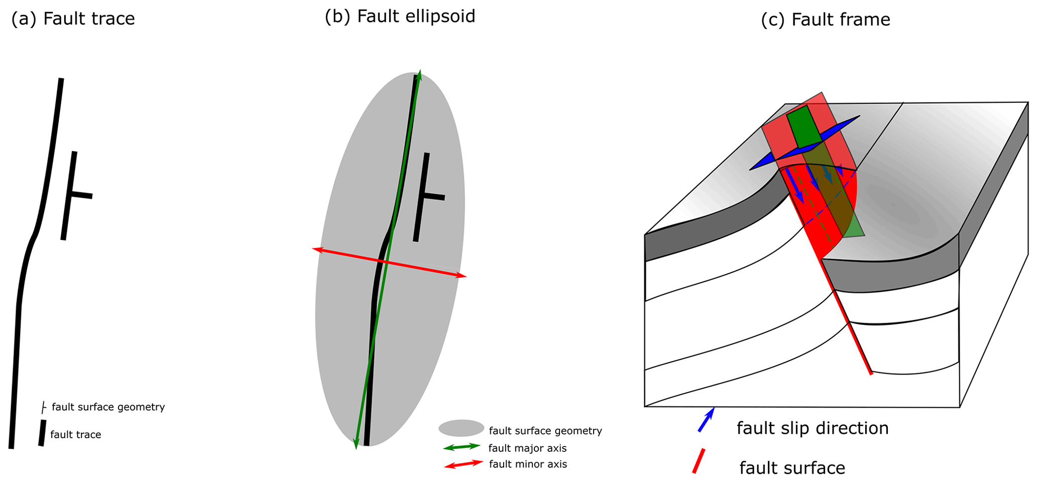
Figure 4 Schematic diagram showing the construction of a fault frame from a fault trace. (a) Fault trace and structural data for fault plane geometry. (b) Fault ellipsoid defined by the major axis and minor axis. (c) Fault frame showing fault surface (red), fault slip (blue) and fault extent (green).

3.2 Fault displacement

The displacement direction of the fault is represented by f₁. The fault displacement magnitude can be either defined by a constant displacement on the hanging wall or by a function of the fault frame coordinates allowing for the fault displacement to be represented relative to a fault origin using a combination of attenuation profiles as described by Laurent et al. (2013) and Godefroy et al. (2018). We define the local fault displacement vector for any location as

$$\begin{array}{}\text{(2)}& {\mathit{f}}_{\mathrm{disp}}=d\cdot {\mathit{f}}_{\mathrm{1}},\end{array}$$

where d is the scalar value of the fault displacement magnitude at that location.

3.3 Time-aware geological modelling

The aim of implicit 3D geological modelling is to define a function or series of functions that can be evaluated for any location in the model and return some information about the geological feature of interest (either the distance to a feature, e.g. lithological contact or fault surface, or the orientation of the feature) (Wellmann and Caumon, 2018). This means that the resulting geological model can effectively be represented by an ordered list of mathematical functions. The topological relationship between these mathematical functions should be related back to the geological topology, e.g. the overprinting relationships between geological events.

To represent a faulted geological feature, we first define the geological feature in the model using the associated structural data. A fault can then be applied to this geological feature which produces a faulted geological feature. The fault restores the observations attached to the faulted geological feature to their location using the fault kinematics from the fault operator. The faulted geological feature can then be interpolated using the restored locations. To evaluate the scalar field of the faulted geological feature the fault transformation must be added to the implicit surface representation. This is done by applying the fault restoration kinematics to the data points prior to evaluating the scalar field values.

$$\begin{array}{}\text{(3)}& {\mathit{\varphi }}_{\mathrm{faulted}}(x,y,z)={\mathit{\varphi }}_{\mathrm{base}}\left({\mathit{f}}_{\mathrm{disp}}\left(x,y,z\right)\right)\end{array}$$

Using this workflow, it is possible to stack multiple fault operators and apply, backwards in time, the appropriate displacements to restore the location to its position prior to faulting. Where faults do not intersect, the relative timing does not need to be known, and these faults can be modelled simultaneously. This approach can be applied to any structural elements in the model, including lineations, fold vergence, tectonic foliations and fold frames (Grose et al., 2017).

4 Implementation

The generalised workflow presented above does not depend on the specifics of the interpolation scheme. We present an overview of how to build the fault frame using discrete interpolation algorithms using LoopStructural (Grose et al., 2021a), an open-source 3D modelling library (https://github.com/Loop3D/LoopStructural, last access: 29 September 2021). Using discrete interpolation algorithms, the complexity of the interpolation problem is defined by the resolution of the support and not by the number of constraints.

4.1 Building fault frame

The fault frame is built by interpolating the scalar fields using the following procedure:

1. Interpolate coordinate 0 to represent the geometry of the fault surface so that the isosurface of 0 contains the fault trace and the field is parallel to the orientation of the fault surface.

2. Interpolate coordinate 1 so that the direction of its gradient norm is orthogonal to the direction of the gradient norm of the fault surface and parallel to any kinematic indicators for the fault.

3. Interpolate coordinate 2 so that the direction of its gradient norm is orthogonal to the direction of the gradient norm of the fault surface field and to the fault slip direction field.

In this study, we use a discrete implicit modelling technique where the implicit function is represented on a discrete support either by a piece-wise linear function on a tetrahedral mesh (Mallet, 2002; Frank et al., 2007; Caumon et al., 2013; Grose et al., 2021a) or by using finite differences on a Cartesian grid where an objective function such as the bending energy (Renaudeau et al., 2019) or the second derivative is minimised (Irakarama et al., 2020). To build the fault frame, an additional constraint needs to be applied to the interpolation to ensure that the fault slip direction and fault extent fields are orthogonal. To add this additional constraint the gradient of an existing component of the fault frame (∇f_i) (for example the gradient of the fault surface) is obtained for every element in the mesh, and this gradient norm is then used to constrain the interpolation of a new field (∇f_j) so that the gradient norm of the new field is orthogonal to the gradient norm of the existing field.

$$\begin{array}{}\text{(4)}& \mathrm{\nabla }{f}_i\cdot \mathrm{\nabla }{f}_j=\mathrm{0}\end{array}$$

The scalar field can then be interpolated by minimising the misfit between the orthogonality constraint and any observations of the fault slip direction. If the fault being modelled has a constant displacement along on coordinate, this coordinate can be obtained by finding the vector product between the other two fields.

The element orthogonality constraint can be applied to two fields and the resulting scalar field will be close to orthogonal to both. Frequently it is difficult to measure or observe the fault slip direction. In these cases, the geologists would need to use qualitative geological knowledge to define the fault slip direction using their knowledge about the geology of the area. It is also possible to build the model with different fault slip directions (and magnitudes) in order to explore the range in possible geometries and compare these with observations.

4.2 Volumetric fault displacement

Fault slip is defined by three functions applied to the normalised fault frame coordinates. Where the fault is active the fault frame coordinates will be between −1 and 1 and be equal to −1 or 1 where the fault is inactive. The same approach for combining the fault profiles within the fault frame is used to define a volumetric fault displacement field as Godefroy et al. (2018), which was adapted from Laurent et al. (2013):

$$\begin{array}{}\text{(5)}& \mathit{\delta }\left(X\right)=D_{\mathrm{0}}\left(f_{\mathrm{0}}\right(X\left)\right)\cdot D_{\mathrm{1}}\left(f_{\mathrm{1}}\right(X\left)\right)\cdot D_{\mathrm{2}}\left(f_{\mathrm{2}}\right(X\left)\right),\end{array}$$

where $D_{\mathrm{0},\mathrm{1},\mathrm{2}}$ denotes 1D curves describing the displacement of the fault within the fault frame.

A unit vector representing the displacement direction (e_d) can be locally obtained using the fault frame coordinates. We use the local direction vector e_d(X)⋅δ(X) to define the local slip vector for the fault. This scaled displacement field is calculated for the entire model support and can then be queried for the local model of interest. Faults can be integrated into the implicit function by restoring locations using the scaled displacement field. Where the fault geometry is not planar, the fault restoration is applied using Euler's method, where the displacement is applied iteratively using small linear steps. Applying the displacement iteratively ensures that the relative position of the restored locations is maintained.

4.3 Splay faults

Faults are rarely single surfaces and are often defined as fault zones with complex linkage between individual fault segments. During the development of a fault zone, an individual surface can splay, meaning that the fault offset is partitioned onto multiple slip surfaces (Huggins et al., 1995; Marchal et al., 2003). The resulting geometries can be increasingly complex and include duplexes and flower structures.

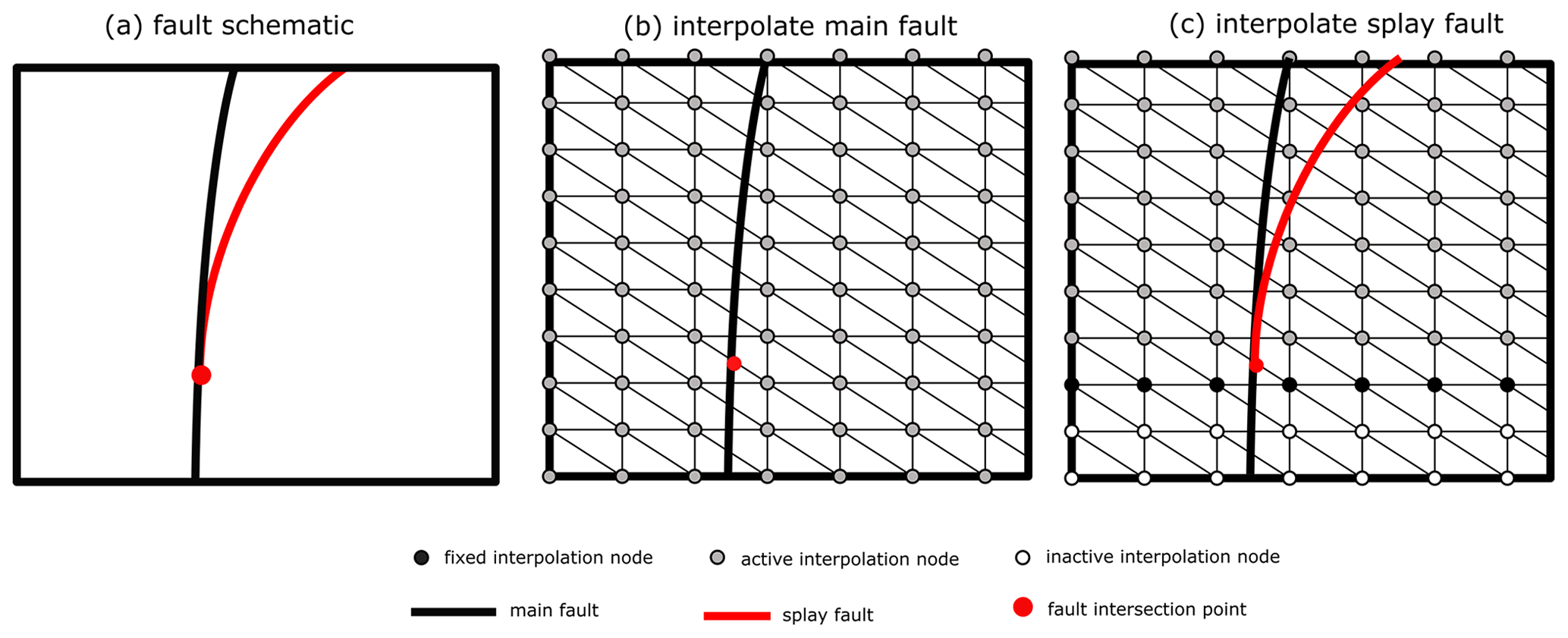
Figure 5 Schematic diagram showing interpolation of splay faults. (a) Fault diagram showing the observations of the main fault (blue dots) and splay fault (red dot). The splay region is represented by the rectangle with the diagonal lines) (b) Interpolation support for main fault showing fault geometry and all interpolation nodes being active. (c) Interpolation of splay fault showing fixed, active and inactive interpolation nodes where the fault geometry is shared.

An advantage of our approach is that multiple faults can be applied sequentially where the total displacement is defined by the accumulation of the local displacement fields. Modelling faults in a time-aware approach is similar to how folds are modelled (Laurent et al., 2016; Grose et al., 2017, 2018) where the most recent fold is modelled first and this defines the geometry of the folded foliations.

A fault zone can be represented by a piece-wise combination of fault segments. To model multiple connected faults, the fault frames need to equal along the branch line. In the following section, hard constraints are incorporated into the interpolation system using Lagrange multipliers.

Discrete interpolation approaches define the interpolation within a volume of interest by a linear system where the unknowns are the property values on the mesh nodes (Frank et al., 2007; Caumon et al., 2013). The unknowns are found by solving the linear system:

$$\begin{array}{}\text{(6)}& \mathbf{A}\cdot \mathit{x}=\mathit{b},\end{array}$$

where A​​​​​​​ is an interpolation matrix that contains the different geological constraints (contact observations, orientation constraints, orthogonality constraints) and a regularisation term that controls the smoothness of the resulting scalar field, and x denotes the values of the scalar field at the interpolation nodes. The linear system defined in Eq. (6) is over-determined and can be solved in a least-squares sense by minimising the L-2 norm $\left|\right|\mathbf{A}\mathit{x}-\mathit{b}|{|}_{\mathrm{2}}^{\mathrm{2}}$​​​​​​​.

Splay faults (Fig. 5a) share the same geometry as the parent fault at the point of intersection. To ensure the faults share the same geometry an additional constraint needs to be added to the linear system so that the scalar field value of the shared nodes of the fault are equal. In Fig. 5b the main fault is interpolated using all interpolation nodes. To interpolate the splay faults the hard constraints need to be identified by finding the values of the fault extent field (f₂) where the fault is active. Equality constraints are identified by finding the elements that contain the isosurface of the fault extent field containing the intersection point, i.e. black nodes in Fig. 5c. The hard constraints form an additional linear system,

$$\begin{array}{}\text{(7)}& \mathbf{C}\cdot \mathit{x}=\mathit{d},\end{array}$$

where C is the interpolation matrix for the equality constraints.

To solve this system, ensuring that the hard constraints are strictly honoured and the other interpolation constraints are satisfied in a least-squares sense, we define the Lagrangian for the least-squares problem,

$$\begin{array}{}\text{(8)}& \mathcal{L}(x,\mathit{\lambda }):={\displaystyle \frac{\mathrm{1}}{\mathrm{2}}}\left|\right|\mathbf{A}\mathit{x}-\mathit{b}|{|}_{\mathrm{2}}^{\mathrm{2}}+{\mathit{\lambda }}^T(\mathbf{C}\mathit{x}-\mathit{d}),\end{array}$$

where λ denotes the Lagrange multipliers. To apply this constraint we need to know where the two faults share geometries so that the values of the main fault can be used as equality constraints to interpolate the splay fault. Where the geometry of the two surfaces is shared, the property value of the nodes inside the shared region are fixed so that both surfaces have the same value (Fig. 5c). This can be implemented where ${\mathbf{C}}_{i,j}=\mathrm{1}$, where i is index of hard constraint and j is the node global index. d_j is equal to the shared node value between the two scalar fields. Alternatively, the hard constraints could be defined using the discrete support shape functions (e.g. linear tetrahedron or trilinear interpolation); however, in this case the line of intersection would need to be known, which may be complicated or impossible to quantify.

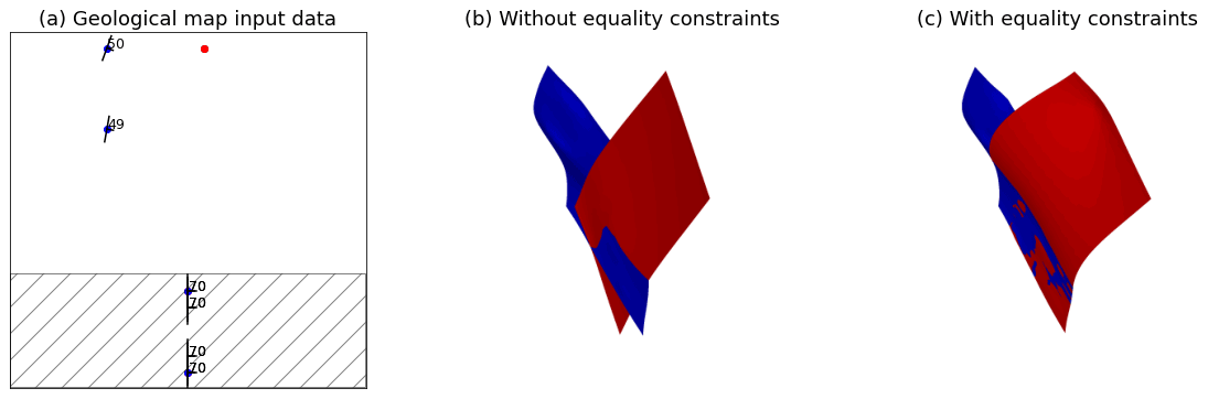
Figure 6 Comparison of fault surfaces modelled using equality constraints and without equality constraints. (a) Input datasets showing observations for both faults. The blue dots represent the location of the main fault and the red dot represents the location of the splay fault. The rectangle represents the area where the faults share the same geometry. (b) Fault surfaces modelled without equality constraints. (b) Fault surfaces modelled with equality constraints.

In Fig. 6b and c, two splay faults are interpolated. In (b) the same constraints are used to solve both surfaces, and the resulting faults overlap but do not share the same geometry in the region where they are expected to splay. In (c) equality constraints are used to constrain the surface geometry to be the same before the fault splay (shown by the rectangle in Fig. 6a). When modelling complex fault networks, for example splay faults or other faults with shared geometries, the hard constraints ensure that the faults have the same geometry at intersection lines. For splay faults this will also ensure that the interpolation of the splay fault also includes the parent fault geometry.

5 Case studies

In the following sections we present three synthetic case studies that demonstrate the application of our approach to both extensional and contractional systems. All of the case studies have been implemented in the open-source 3D structural modelling library, LoopStructural 1.2.0 (https://doi.org/10.5281/zenodo.5234619, Grose et al., 2021b, a). The case studies are provided as interactive Jupyter notebooks in https://doi.org/10.5281/zenodo.5234634 (Grose, 2021).

5.1 Faulted intrusion

The first case study is a synthetic intrusive body that has been faulted by a planar normal fault. The intrusion has been randomly sampled with one set of data points describing the distance to the intrusion surface where the value is 0 and another set of data points where the value is 1, which describes the distance to the intrusion surface. In Fig. 7a the observations of the faulted surface are shown along with the interpolated fault surface. The fault displacement is pure dip slip with a normal sense, meaning the points on the hanging wall (left side) have been displaced down. A vector field representing the fault restoration is defined by multiplying the fault slip direction field (orthogonal to the fault surface and parallel to observations of the fault slip) by the fault displacement magnitude. In this example a fault displacement of 500 m is used. Figure 7b shows the fault displacement vector field applied to the data points on the hanging wall of the fault, indicating the direction of movement to restore the data points to their location prior to faulting. The data points that are identified as being on the footwall of the fault are not affected by the fault restoration and are grey coloured without a vector field. Figure 7c shows the data points from Fig. 7a in the restored locations after applying the fault operator. The intrusion shape is interpolated within the restored space (Fig. 7c, d) using a discrete interpolation approach with a weak regularisation constraint to allow for the propagation of a high curvature geometry. A weak regularisation constraint is applied because modelling intrusions with implicit interpolation approaches has similar challenges to modelling folds (Laurent et al., 2016), where high curvature is expected but the interpolation actually minimises the curvature. A kinematic operator is added to the interpolated scalar field so that when evaluating the scalar field at a location, the location is restored using the fault displacement field. Figure 7e shows the model support for a regular grid where the points in the hanging wall are restored using the restoration vector field. In practice, the points are not actually moved and the restoration vector field is actually added to the implicit surface description, resulting in a faulted intrusion (Fig. 7f).

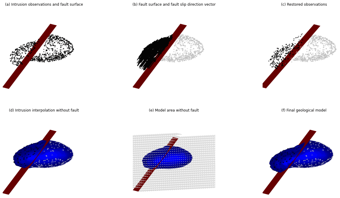
Figure 7 Case study showing faulted 3D intrusion. (a) Observations of the intrusion surface (black points) and modelled fault surface (red surface). (b) Fault restoration vector evaluated on data point locations showing the restoration direction. (b) Restored data points from A. (d) Intrusion surface interpolated in restored domain showing data points and fault surface. (e) Regular grid highlighting restoration function on model domain, where the hanging wall points have been restored. (f) Fault and faulted intrusion surfaces.

In this example, the intrusion volume is maintained when the fault is applied. The volume of an intrusion when modelled using step functions is likely to change as shown in Fig. 2.

5.2 Finite fault

In the previous examples, we have shown a constant displacement on the hanging wall of the faults. Applying a constant displacement implies making the assumption that the fault displacement is uniform across the fault and that the faults are infinite throughout the model area. This assumption of uniformity is useful where the faults extend across the model domain. In contrast many faults end within the model region of interest, and these should be represented as finite features.

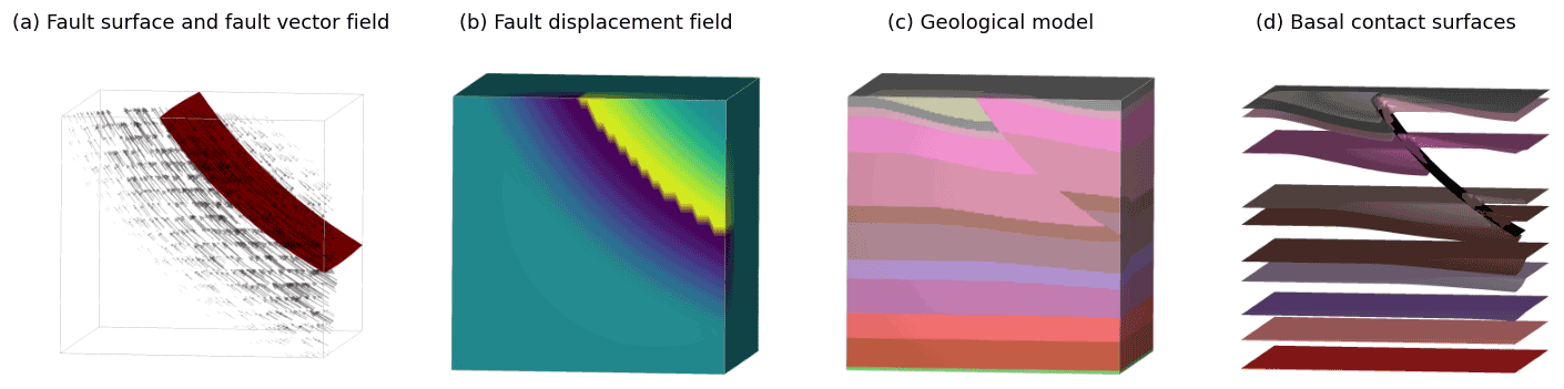
Figure 8 Finite fault applied to flat-lying stratigraphy. (a) Fault displacement vectors and isosurface of fault surface scalar field. (b) Scalar field of fault displacement. (c) Geological model showing unit distributions for stratigraphy. (d) Surfaces of stratigraphy.

To model finite faults the fault displacement needs to vary relative to the proximity to the fault. The volumetric displacement can be defined by combining three 1D displacement functions that describe the fault displacement as a function of the fault frame coordinates. The fault frame coordinates need to be normalised so that they range from −1 to 1 within the fault ellipsoid, the volume defined by non-zero fault displacement. The profile of the fault displacement in f₀ defines the geometry of the fault throw. The profile of the fault displacement in f₁ defines the magnitude of the displacement along the fault slip direction (e.g. how deep does the fault extend for a dip-slip fault) and the fault displacement profile in f₂ describes the magnitude of the displacement along the major axis of the fault surface.

In Fig. 8a the fault surface is shown with the slip vectors within the fault volume scaled by the displacement magnitude. The corresponding fault displacement fields are shown in Fig. 8b. In this example the fault has maximal displacement in the centre of the fault decreasing to the extents of the fault ellipsoid defined by 1D functions in each of the fault frame coordinates. Different profiles can be chosen either to fit observations or to enforce a particular conceptual model.

The resulting 3D displacement scalar field is shown in Fig. 8b, where displacement scales from 0 to ±1 close to the fault. This displacement field and the fault slip direction vector field can be added to the implicit surface scalar field (shown in Fig. 8c). Figure 8d shows the faulted stratigraphic surfaces where the implicit function is evaluated using the fault restoration function. In Fig. 8b and d the displacement of the fault decreases away from the fault and at depth, with the displacement not affecting the lowest contact. In Fig. 8c displacement of the fault decreases along the fault with no displacement occurring on the tip of the fault.

5.3 Thrust duplex

Figure 9 is a synthetic case study of a thrust duplex. The observations of the fault surfaces are shown in Fig. 9a, where the red dots represent the observations of the younger fault location and both blue dot and red dots represent the observations of the older fault location. The fault network shows ramp and flat geometry that is commonly found in compressional settings.

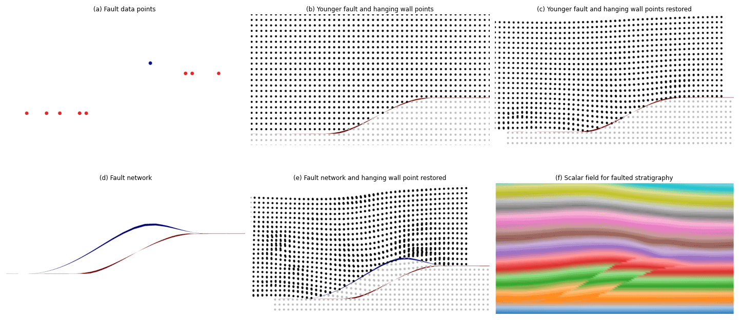
Figure 9 Fault duplex applied to flat-lying stratigraphy. (a) Observations of the fault surfaces with red dots showing the location of both surfaces and the blue dot showing the location of the older fault. (b) Younger fault surface interpolated with model domain showing hanging wall (black) and footwall (opaque) points. (c) Hanging wall points restored by younger fault restoration function. (d) Surfaces for older fault and younger fault. (e) Model restored by both faults with hanging wall of older fault highlighted by black points. (f) Duplex fault network added to scalar field of bedding.

The younger fault is modelled first by interpolating the observations associated with this fault; the resulting surface is shown in Fig. 9b. In Fig. 9b the model domain is highlighted by the black (hanging wall) and opaque points (footwall). The kinematics of the younger fault are applied to the model nodes shown in Fig. 9c where the kinematics are applied in reverse and hanging wall nodes have been restored. The younger fault splays from the older fault where the ramp occurs, and both faults share the same geometry at the flat (defined by the red data points). To ensure that the geometry of the interpolated surfaces is the same at the flats the overlapping interpolation nodes from the younger fault are used as equality constraints for the older fault interpolation. The older fault surface observation (blue dot) is restored to its original location and the surface is interpolated, combining this observation and the equality constraints from shared geometry of the flats. The younger fault is added to the implicit function of the older fault, and both faults are shown in Fig. 9d. The older fault shows a fault bend fold that is the result of the movement of the younger fault.

To demonstrate the combined kinematics of this fault network the faults are added to the implicit function representing flat-lying stratigraphy (Fig. 9f). On the footwall of the younger fault the layers are flat-lying and there is no deformation. Between the younger and older fault there is a horst where there is minor rotation of stratigraphy. Above the older fault there is a fault bend fold that can be seen in the stratigraphic layers. These geometrical features are all resulting from the modelled fault kinematics and not mechanics.

5.4 Faulted fold series

In the final example, we model a faulted doubly plunging fold. The reference model was generated using Noddy (Jessell and Valenta, 1996) and the orientation of the fault surface, fold axial surfaces and folded surface were sampled at irregular locations shown in the geological map (Fig. 10).

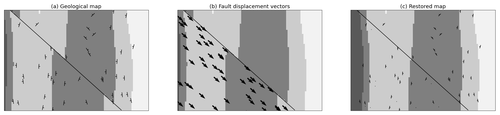
Figure 10 Geological map showing (a) structural observations for bedding, (b) interpolated fault restoration vectors and (c) a restored map.

To model folded and refolded structures we use the framework introduced by Laurent et al. (2016) and Grose et al. (2018). To model the faulted fold series the most recent structure needs to be modelled first. In this case this is the fault as it overprints the fold series. We model the fault frame by first interpolating the fault surface using observations of the fault surface (fault trace and fault dip). The fault slip direction is then interpolated so that the gradient of the fault slip field is parallel to the fault slip observations and orthogonal to the gradient of the fault surface. The fault extent can then be interpolated so that its gradient is orthogonal to both the fault slip and the fault surface gradients. The fault trace (black line) and fault slip vectors (black arrows) are shown in Fig. 10b. In this example the reference model fault displacement of 1000 m is used to define the fault displacement.

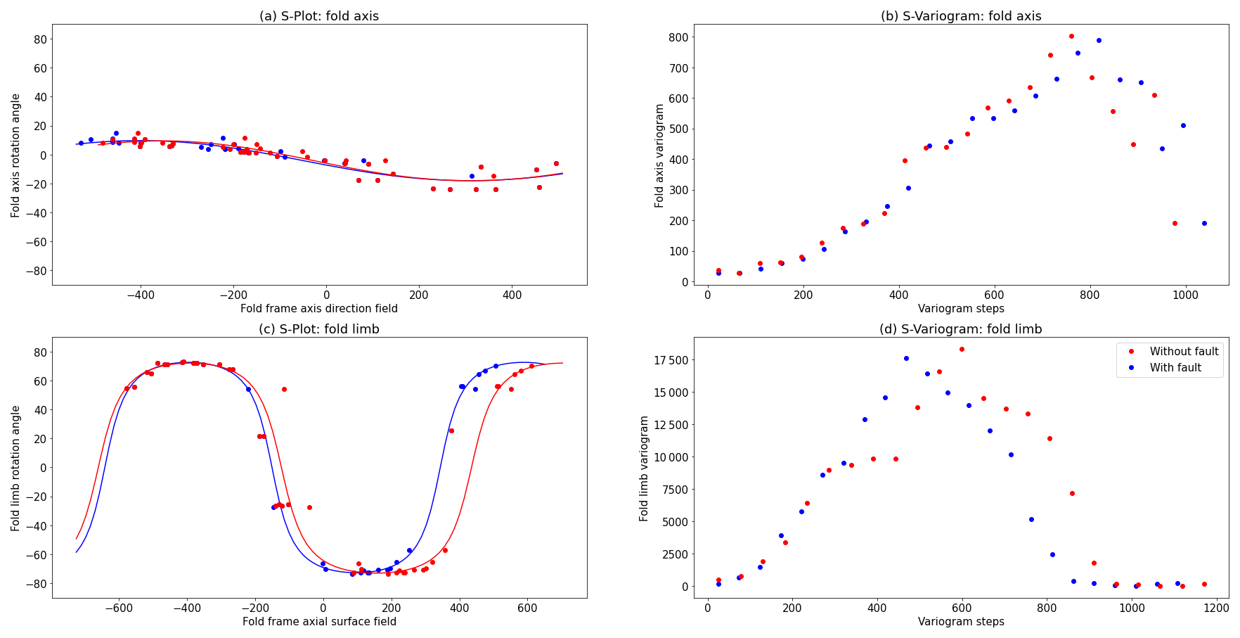
Figure 11 Fold geometry plots for the fold axis geometry and fold limb geometry. (a) S plot showing the variation in fold axis rotation angle with respect to the fold axis direction field showing the fold axis with and without the fault. (b) S variogram of the fold axis rotation angle. (c) S plot of the fold limb rotation angle with and without the fault. (d) S variogram of the fold limb rotation angle.

The fold frame for F1 is interpolated in a similar way to the fault frame, by first interpolating the axial foliation and then interpolating the fold axis direction field (Laurent et al., 2016). The fault is added to the fold frame meaning that the interpolation of the fold frame occurs after the observations have been restored. The scalar fields for the fold frame can be seen in Fig. 12a and b.

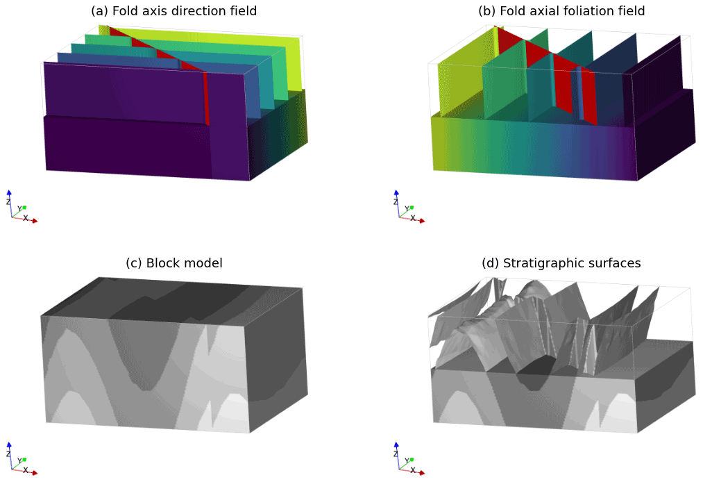
Figure 12 Example integrating fault kinematics and fold modelling from Laurent et al. (2016) and Grose et al. (2017). (a) Fold frame axial foliation scalar field. (b) Fold frame fold axis direction scalar field. Corresponding fold S plots are shown in Fig. 11. (c) Scalar field showing bedding interpolated using fold constraints with the fault added to the interpolator. (d) Surfaces extracted from the geological model in (c) including the fault surface.

Within the fold frame, the intersection lineation is calculated by finding the cross product between the normal to observations of bedding and the gradient of the interpolated axial foliation. The fold axis rotation angle is calculated by finding the angle between the intersection lineation and the fold axis direction field. The fold axis rotation angle is interpolated throughout the model by fitting a Fourier series to the calculated fold rotation angles. We use the Levenberg–Marquardt algorithm for fitting the non-linear least-squares problem implemented in the curvefit function found in the scipy optimise module. The orientation of the fold axis can be locally obtained by rotating the gradient of the fold axis direction field by the fold axis rotation angle. The fold limb rotation angle is calculated by finding the complementary angle to vergence using the interpolated fold axis. Similar to fitting the fold axis rotation angle the fold limb rotation angle is fitted using a Fourier series function and the Levenberg–Marquardt algorithm to find optimal coefficient and wavelength values.

In Fig. 11a the fold axis rotation angles are plotted against the fold axis direction field coordinate (Fig. 12a). The fold axis rotation angle is shown (1) where the fault has been added to the interpolator (as blue dots) and where the fault has not been included (as red dots). This stronger impact can be explained by the fact that the wavelength of the fold limb rotation angle is smaller than that of the fold axis rotation angle. The wavelength of the fold limb rotation angle decreases when removing the effect of the fault, whereas the wavelength of the fold axis rotation angle increases. This highlights that ignoring the fault could lead to biases when characterising the frequency of the folds. The fold axis rotation angle is marginally affected by the fault, because fold axis variations are relatively small and low-frequency as compared to the fault displacement. This low frequency is highlighted by the absence of a hole effect in the S variogram (Fig. 11b), suggesting that there is not a full wavelength of the fold observed in the fold axis. When the fault displacement is applied to the points before fitting the fold axis rotation angle the wavelength is slightly larger (blue curve in Fig. 11), corresponding to a more consistent alignment of the fold hinges across the fault. The blue curve shows the fold axis rotation angle profile fitted to the blue points.

The fold limb rotation angle is plotted against the fold axial foliation field (Fig. 12b) shown in Fig. 11c. In the S plot the limbs of the fold are represented by positive and negative clusters and the locations where the rotation angle crosses 0 are the hinge (Grose et al., 2017). There are three limbs observed in the data points, one around an axial foliation value of −2, another around an axial foliation value of 0 and a final one around an axial foliation value of 2. Where the fault is added to the interpolator, the limbs at 0 and 2 are shifted towards the limb at −2. In this case, the variation in orientation shown in the S plot could either be explained by adding a fault (as done here) or varying the fold wavelength between fold limbs. The resulting 3D geometry (Fig. 12c and d) shows the location of the fold hinges are offset in the slip direction for the fault.

6 Discussion

A single fault is challenging to incorporate into 3D geological modelling because it defines a discontinuity in the older geological surfaces. This challenge is further complicated because the fault is not only defined by the location of the discontinuity but by the kinematics associated with the displacement of the faulted objects. This means that to properly model faults, the kinematics need to be directly incorporated into the modelling process. These complications are further exaggerated when modelling a fault network where there are multiple overprinting and interacting faults.

In this contribution faults are modelled using a curvilinear coordinate system and fault operator adapted from Laurent et al. (2013) and Godefroy et al. (2018) to directly incorporate fault kinematics into the surface description. Our approach applies the fault operator in reverse prior to interpolating the surface, meaning that the fault description is incorporated into the implicit surface representation rather than applied to an already discretised surface. Both approaches require building a reference coordinate system for the fault that defines the fault surface, fault slip direction and the fault extent. The coordinate system can be easily constrained from observations where the fault slip direction must always be orthogonal to the fault surface and the fault extent is always orthogonal to the fault slip direction and the fault surface. We show that this coordinate system can be built allowing for multiple overprinting and interacting faults to be modelled using a serial approach where the scalar fields representing the coordinates are modelled sequentially. While this approach produces an acceptable coordinate system for the faulting, it can be costly to evaluate, especially in high-resolution models. The following strategies are used in LoopStructural for modelling large fault networks: (1) lower the resolution of the interpolation support for the fault network, as the geometry of the fault should be less complicated than stratigraphy, and (2) only model the fault geometry within the fault volume.

One of the key advantages of our approach is the ability to make use of kinematic observations for constraining the geometry of faulted geological surfaces. However, in a lot of cases (e.g. geological survey maps, potential field geophysical interpretations), the required kinematic indicators are unknown. One approach for solving this problem would be to build the fault frame by aligning the fault surface with observations of the fault surface (this step is no different to any other implicit modelling approach) and second to align the fault extent direction with the map extent of the fault. This defines the fault volume as an ellipsoid where the major axis is aligned with the map pattern of the fault. The fault slip direction is then orthogonal to both of these interpolated fields. This approach would provide a good first pass approach for modelling the fault displacement and is a similar outcome to the inferred slip direction used by step functions, albeit using our approach the fault kinematics are modelled appropriate to the dip of the fault.

One of the challenges for the presented approach is determining the correct displacement magnitude and profile. Although in some cases these parameters are observations recorded on a geological map they are not always present. Godefroy et al. (2018) applies particle swarm optimisation for these parameters by optimising the displacement to the data points within the fault volume. In a similar approach, an objective function could be applied to the restored continuous surface minimising some metric, for example for folding this could be incorporated into the probabilistic geological inversion presented by Grose et al. (2018, 2019). In this framework, fitting a fold model to the S plot could be used to determine whether a displacement parameter and fault profile are acceptable. Figure 11c shows the fold limb rotation angle for the faulted fold series where the fault has been added (blue dots) and where the fault has not been added (red dots). Adding the fault changes the shape of the S plot and could be added as a likelihood function in an inversion framework. As with all geological problems this would be highly uncertain and require additional domain knowledge to result in a solution.

7 Conclusions

The geometry and offset of fault networks is challenging to integrate into implicit 3D modelling algorithms. Directly integrating faults into the implicit description of surfaces using step functions does not allow for kinematic observations to be incorporated and will result in fault geometries with inconsistent kinematics. In order to mask these flaws, it is possible to constraint fault geometries using interpretive constraints. In this contribution the kinematics are applied in reverse to restore the observation into a pre-fault location. Within the restored model space a continuous surface can be evaluated. The interpolation occurs within the restored model space, meaning that no discontinuities or re-meshing are required to generate the models. The restoration kinematics are then added to the implicit description of the model surface, allowing for the surface to be evaluated and capturing the fault location and the kinematics of the fault. Our approach can be applied to parametric modelling of folds where the fault restoration is applied to the fold geometry characterisation. We demonstrate applications to multiple synthetic examples including a faulted doubly plunging fold series. The flexible description of our model geometries allows more sophisticated kinematic models to be integrated into the workflow.