LoopStructural 1.0: time-aware geological modelling

In this contribution we introduce LoopStructural, a new open-source 3D geological modelling Python package (http://www.github.com/Loop3d/LoopStructural, last access: 15 June 2021). LoopStructural provides a generic API for 3D geological modelling applications harnessing the core Python scientific libraries pandas, numpy and scipy. Six different interpolation algorithms, including three discrete interpolators and 3 polynomial trend interpolators, can be used from the same model design. This means that different interpolation algorithms can be mixed and matched within a geological model allowing for different geological objects, e.g. different conformable foliations, fault surfaces and unconformities to be modelled using different algorithms. Geological features are incorporated into the model using a time-aware approach, where the most recent features are modelled first and used to constrain the geometries of the older features. For example, we use a fault frame for characterising the geometry of the fault surface and apply each fault sequentially to the faulted surfaces. In this contribution we use LoopStructural to produce synthetic proof of concepts models and a 86 km × 52 km model of the Flinders Ranges in South Australia using map2loop.

1 Introduction

Understanding and characterising the geometry and interaction between geological features in the subsurface is an important stage in resource identification and management. A surface or combination of surfaces can be used to represent the subsurface geometry of geological features or structural elements within 3D geological models (Caumon et al., 2009). There are two main approaches for representing surfaces in 3D geological models: (1) one in which the surface is represented by directly triangulating control points defining the surface geometry or (2) one in which the surface is extracted as an isovalue or level set of an implicit function (Wellmann and Caumon, 2018). Explicit surface representation in geological modelling refers to manually drawn surfaces and is usually time consuming and requires significant subjective user input because surfaces are usually sculpted to the modellers conceptual idea in a similar way to drawing polylines in geographical information systems or using computer-aided design software. Implicit surface representation involves approximating an unknown function that represents the distance to a geological surface. The implicit function can be queried anywhere throughout the model for the value or gradient of the function. The implicit function is fitted to observations that are used to infer the geometry of a geological surface, for example the distance to the geological surface (for stratigraphic horizons this may be the cumulative thickness) or the gradient of the function (on contact or off contact) observations. The topological relationships between different geological features, e.g. horizons, faults interactions, intrusions and unconformities, are incorporated using multiple implicit functions for different components of the model. Implicit surface representation removes the need to generate surfaces and allows for the geological features to be represented directly by the implicit function value.

All implicit surface modelling techniques involve finding a combination of weighted basis functions that fit the geological observations. There are two main approaches used for implicit surface modelling: (1) data-supported approaches where the basis functions are estimated at the data points (Calcagno et al., 2008a; Cowan et al., 2003; Gonçalves et al., 2017; Hillier et al., 2014; Lajaunie et al., 1997) and (2) discrete interpolation where the basis functions are located on a predefined support (Caumon et al., 2013; Frank et al., 2007; Irakarama et al., 2018; Renaudeau et al., 2019). The algorithms are often linked to commercial software, e.g. Leapfrog¹, 3D GeoModeller² and Gocad-SKUA³. These packages will usually only provide one algorithm for interpolation, making it difficult to compare different interpolation schemes. The algorithms are also usually black box algorithms with limited ability to change algorithm parameters, with no understanding of how the algorithm is implemented. A recent open-source Python library, Gempy (de la Varga et al., 2019), implements the dual co-kriging implicit interpolation algorithm (Lajaunie et al., 1997) using a high performance computational library.

In this contribution we introduce the open-source LoopStructural, a 3D geological modelling Python library based on the incremental contributions of Laurent et al. (2016) and Grose et al. (2017, 2018, 2019). LoopStructural is a new geological modelling engine developed within the Loop⁴ consortium (Ailleres et al., 2018). The core modelling library within LoopStructural depends on scipy (Virtanen et al., 2020), numpy (Van Der Walt et al., 2011) and pandas (pandas development team, 2020), the core scientific Python libraries. A visualisation module uses LavaVu (Kaluza et al., 2020), a minimal OpenGL visualisation package allowing for models to be visualised within a Jupyter notebook environment. LoopStructural has been written using an object-oriented program design with class structures designed to allow for powerful inheritance and modularity. The design of LoopStructural allows development and research into geological modelling methods to be easily performed without having to rewrite boiler plate code for interpolation algorithms, visualisation and model interaction. LoopStructural is a modelling package allowing for multiple stratigraphic groups, faults, folds and unconformities to be represented using implicit surfaces. Different interpolation algorithms can be used for interpolating these surfaces with the ability to mix and match interpolation algorithms depending on the surface type being modelled. LoopStructural has native implementation of discrete implicit modelling using a piecewise linear interpolation on a tetrahedral mesh (Caumon et al., 2013; Frank et al., 2007; Mallet, 2014, 2002), finite-difference interpolation on a Cartesian grid (Irakarama et al., 2018; Renaudeau et al., 2018), fold interpolation using tetrahedral meshes (Laurent et al., 2016) and an interface to a generalised radial basis interpolation (Hillier et al., 2014).

This paper begins with a background analysis of 3D modelling methods and the algorithms used in implicit modelling, with an overview of the mathematical and geological backgrounds used in our implementation. A detailed overview of the specifics of the implementation can be found on (http://loop3d.github.io/LoopStructural, last access: 15 June 2021). To demonstrate the versatility of LoopStructural and to provide a user guide we include four case studies in this paper with corresponding Jupyter notebooks. The first case study is a synthetic example interpolating two planar surfaces where the height of one surface has been perturbed to simulate uncertainty in the surface location. In this example we use the LoopStructural API to compare three different interpolation codes and investigate the parameters and how they are affected by noise. The second example is a synthetic refolded type 3 interference pattern from Laurent et al. (2016), where we apply the time-aware discrete fold interpolation method described by Laurent et al. (2016) for modelling the refolded folds. In the third case study LoopStructural is applied to a real dataset from the Flinders Ranges in South Australia, where the dataset has been prepared using the pre-processing module of the Loop workflow map2loop (Jessell et al., 2021). In the fourth and final case study we use map2loop to augment an input dataset for a model in the Hamersley region in Western Australia. We generate 10 unique models, demonstrating the range of possible geometries when perturbing the fault geometry.

2 Materials and methods

A 3D geological model can be represented by a collection of surfaces representing geological features (e.g. fault surfaces, stratigraphic horizons, axial surfaces of folds, unconformities) (Wellmann and Caumon, 2018). There are two main tasks for a 3D modelling software package:

• the creation of the surfaces from geological observations and knowledge, this is known as interpolation;

• the incorporation of geological concepts into the surface description, e.g. faulted surfaces should show displacement and unconformities should be a boundary between units.

In LoopStructural surfaces are implicitly represented by an isovalue of one or more volumetric scalar fields (Calcagno et al., 2008a; Caumon et al., 2013; Cowan et al., 2003; Frank et al., 2007; Gonçalves et al., 2017; Hillier et al., 2014; Jessell, 1981; de la Varga et al., 2019; Lajaunie et al., 1997; Mallet, 2002, 2014; Manchuk and Deutsch, 2019; Maxelon et al., 2009; Moyen et al., 2004; Renaudeau et al., 2019; Yang et al., 2019). The geological rules are managed by adding the geological event (folding event, one fault, another fault, an unconformity) structural parameters in a time-aware approach, where the most recent event is added first and the constraints are added backwards in time. Complex geological features such as folds and faults are integrated into LoopStructural by building a structural frame around the principal structural directions of the feature being modelled. Using these structural frames geological rules can be integrated into the modelling workflows – e.g. fault kinematics can be added to the faulted feature because the fault geometry is known before interpolating the faulted feature or fold overprinting relationships can be incorporated using multiple structural frames (Laurent et al., 2016).

2.1 Implicit surface modelling

Implicit surface modelling involves the representation of the geometry of a geological feature using a function f(xyz) where the value of the function is the same along the observation of the surface. There are two possible ways of framing this question. The first approach uses the scalar field value as a distance from a reference horizon, e.g. the location of the horizon for a single surface would be the value of the scalar field. Using this approach, which we will call the signed distance approach, the same implicit function can represent conformable horizons where the value of each horizon is the cumulative thickness from the base of the series (Caumon et al., 2013; Hillier et al., 2014; Jessell, 1981; Manchuk and Deutsch, 2019; Wellmann and Caumon, 2018). The second approach, often referred to as the potential field approach, does not specify the value of the scalar field. The potential field approach only defines the potential field to have the same value for specific interfaces, such as contacts between geological units and fault traces (Calcagno et al., 2008a; de la Varga et al., 2019). As with the signed distance field, the potential field can represent conformable horizons – where the value of the implicit function evaluated on the input observations can be used to infer the potential field value for these horizons.

These implicit functions have no known analytical solution, which means that they need to be approximated from the observations that are provided. The implicit function is represented by a weighted combination of basis functions:

$$\begin{array}{}\text{(1)}& f\left(xyz\right)=\sum _{i=\mathrm{0}}^N{w}_i\cdot {\mathit{\phi }}_i(x,y,z),\end{array}$$

where N is the number of basis functions, w are the weights and φ are the basis functions. There are two approaches for approximating the implicit function: the first approach uses a discrete formulation for the interpolation where N is defined by some sort of mesh (Caumon et al., 2013; Frank et al., 2007; Mallet, 1992; Moyen et al., 2004), and the second approach uses data-supported basis functions where N is defined by the number of data points (Calcagno et al., 2008a; Cowan et al., 2003; Gonçalves et al., 2017; Hillier et al., 2014; de la Varga et al., 2019; Lajaunie et al., 1997).

2.1.1 Input data

Geological observations that are directly incorporated into 3D modelling can generally be divided into two categories: observations that describe the orientation of a geological feature (on contact and off contact) and observations that describe the location within a geological feature (cumulative thickness for conformable stratigraphic horizons, or location of fault surface). In the context of a geological map, location observations may be the trace of a geological surface on the geological map, or a single point observation at an outcrop or from a borehole. Orientation observations generally record a geometrical property of the surface – e.g. a vector that is tangential to the plane or the vector that is normal to the plane (black and dashed arrows in Fig. 1).

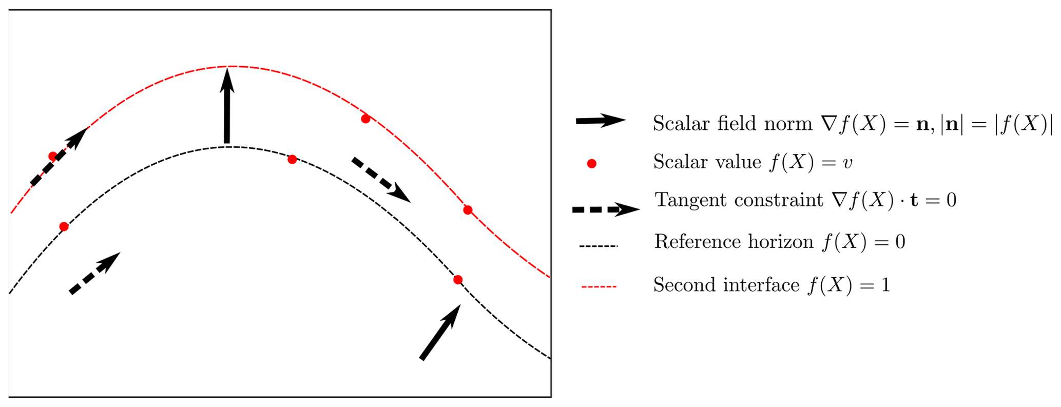
Figure 1 Schematic showing different types of interpolation constraints that can be applied to an implicit interpolation scheme in 2-D. There are two interfaces: the reference horizon with a value of 0 and the next interface with a value of 1. Here we show three types of constraints: (1) scalar field norm constraints constrain the orientation of the scalar field and the norm of the implicit function at that location; (2) scalar field value constraints control the value of the scalar field; and (3) tangent constraints constrain only the orientation of the implicit function not the norm. Figure adapted from Hillier et al. (2014).

When modelling using the potential field approach, the value of the scalar field is inferred through the magnitude of the normal control points. Using the signed distance approach, the value of the scalar field is defined by the value of the observations and effectively controls the thickness of the layers. Orientation constraints either control a component of the orientation, e.g. specifying that the gradient of the function should be orthogonal to the observation or constrain the magnitude and direction of the norm of the gradient of the implicit function.

All geological observations constrain a component of the implicit function at a location in the model:

• Observations for the location of the geological feature will constrain the value of the scalar field $f\left(x,y,z\right)=v$.

• Observations for the orientation of the contact can either

  •

  constrain the partial derivatives of the function $\mathrm{\nabla }f\left(x,y,z\right)=\mathit{n}$ or

  •

  constrain a vector which is parallel to the contact $\mathrm{\nabla }f\left(x,y,z\right)\cdot \mathit{t}=\mathrm{0}$.

It is worth noting that when constraining the partial derivative of the scalar field, the norm of the vector defines the norm of the implicit function which controls the distance between isosurfaces. The sign of the vector must be consistent with the polarity of the structural observation, e.g. for bedding this must be the younging direction. Structural orientations can also be incorporated into the model using two tangent constraints where ${\mathit{t}}_{\mathrm{1}}\times {\mathit{t}}_{\mathrm{2}}=\mathit{n}$, where × is the vector product. In the following sections we will outline the theoretical background for the piecewise linear interpolation, finite-difference interpolation and data-supported interpolation. Within all approaches, the observations are incorporated by adding observations as constraints into a linear system of equations.

2.1.2 Piece-wise linear interpolation

The volumetric scalar field is defined by a piece-wise linear function on a volumetric tetrahedral mesh. In LoopStructural the volumetric tetrahedral mesh creation is simplified by subdividing a regular Cartesian grid into a tetrahedral mesh where one cubic element is divided into five tetrahedra (see Appendix A). The linear tetrahedron is the basis of the piecewise linear interpolation algorithm, where the property within the tetrahedron is interpolated using a linear function; see Appendix A for a detailed description of the linear basis function. We use constant gradient regularisation (Caumon et al., 2013; Frank et al., 2007; Mallet, 1992), where the change in gradient of the implicit function is minimised between tetrahedra with a shared face. The constant gradient regularisation is as follows:

$$\begin{array}{}\text{(2)}& \mathrm{\nabla }{\mathit{\phi }}^{\mathrm{T}\mathrm{1}}\cdot \mathit{n}-\mathrm{\nabla }{\mathit{\phi }}^{\mathrm{T}\mathrm{2}}\cdot \mathit{n}=\mathrm{0},\end{array}$$

where ∂φ^T1 is the gradient of the first tetrahedron, ∂φ^T2 is the gradient of the second tetrahedron and n is the normal vector to the shared face.

2.1.3 Finite-difference interpolation

The second discrete interpolation approach approximates the interpolant using a combination of tri-linear basis functions on a Cartesian grid. The basis functions describe the interpolation as a function of the corners of the cell within which the point where the function is to be estimated falls; see Appendix B for the trilinear basis functions. For example, to evaluate the value of the implicit function at a point x_iy_iz_i, first the cell c is found using integer division of the point coordinates and the grid step vector, where the integer corresponds to the index of the cell in the grid. The local coordinates (ξ, η, ζ) are determined by finding the relative location of the point within the cell. Different regularisation terms can be used; for example Irakarama et al. (2018) minimise the sum of the second derivatives:

$$\begin{array}{}\text{(3)}& {\displaystyle \frac{{\partial }^{\mathrm{2}}}{{\partial }_{xx}}}+{\displaystyle \frac{{\partial }^{\mathrm{2}}}{{\partial }_{yy}}}+{\displaystyle \frac{{\partial }^{\mathrm{2}}}{{\partial }_{zz}}}+\mathrm{2}{\displaystyle \frac{{\partial }^{\mathrm{2}}}{{\partial }_{xy}}}+\mathrm{2}{\displaystyle \frac{{\partial }^{\mathrm{2}}}{{\partial }_{yz}}}+\mathrm{2}{\displaystyle \frac{{\partial }^{\mathrm{2}}}{{\partial }_{zx}}}=\mathrm{0}.\end{array}$$

Alternatively, a partial differential equation such as the bending energy (Renaudeau et al., 2019) or Gaussian curvature could be used. In LoopStructural 1.0, currently only the sum of the second derivatives can be used. The object-oriented program design would allow for different regularisation constraints to be implemented without requiring any boiler plate code.

2.1.4 Solving discrete interpolation

Using either the piecewise linear interpolator or the finite-difference interpolator the scalar field is defined by the node values of the support. These can be found by solving a system of equations with M unknowns $x_{\mathrm{1}},\mathrm{\dots },x_M$ (Caumon et al., 2013; Frank et al., 2007; Mallet, 2004). The unknowns can be found by solving the linear system of equations:

$$\begin{array}{}\text{(4)}& \mathbf{A}\cdot x=\mathit{b},\end{array}$$

where A is an N×M sparse matrix containing the linear constraints and b the right-hand side vector containing the observation of constraint value. For example, to integrate value observations the row in the interpolation matrix A would contain the shape parameters for the cell in which the point is contained. The right-hand side would be the value of the scalar field.

The interpolation problem is over-constrained, i.e. N>M, and can be solved in a least squares sense. The least squares problem can be solved using a number of different algorithms either directly where A^T⋅A is directly inverted, e.g. using lower–upper decomposition, or using an iterative algorithm such as conjugate gradient. Generally, for large problems an iterative approach is recommended because it requires less memory. LoopStructural allows for multiple different solvers to be used for the least squares problem. The default solver is the conjugate gradient algorithm implemented in scipy. To speed up the solver and in some cases improve the stability of the solution we provide the option of adding a small value (the smallest representable float) to the diagonal of the square matrix (A^T⋅A).

2.1.5 Data-supported interpolation

Another approach for implicit surface modelling is to use basis functions that are located at the same location as data points.

This can be done using radial basis interpolation where the interpolation problem is attempting to approximate the signed distance field:

$$\begin{array}{}\text{(5)}& f\left(x,y,z\right)=\sum _{i=\mathrm{0}}^N{w}_i\cdot \mathit{\phi }\left(X\right)+P(x,y,z).\end{array}$$

Alternatively, the problem can be represented using dual co-kriging (Calcagno et al., 2008b; de la Varga et al., 2019; Lajaunie et al., 1997), where the interpolation algorithm estimates the potential field, which estimates incremental differences between the scalar field for different horizons. Using this approach, the system is separated into two parts: (1) the orientation observations which are incorporated using the direction and magnitude and (2) the difference between the potential field for different horizons.

LoopStructural uses SurfE, a C++ implementation of the generalised radial basis interpolation (Hillier et al., 2014) for all data-supported interpolations. SurfE has three approaches for implicit surface reconstruction (1) signed distance interpolation using radial basis functions, (2) potential field interpolation using dual co-kriging (Lajaunie et al., 1997) and (3) signed distance interpolation using a separate scalar field for each surface. The interface between LoopStructural and SurfE allows the user to access all of the interpolation parameters used by SurfE. These include access to more sophisticated solvers, as well as the addition of a smoothing parameter into the interpolation.

2.2 Modelling geological features

There are three ways that the geometry of rock packages can structurally interact in a geological model:

1. stratigraphic contacts – the contact between sedimentary layers;

2. fault contacts;

3. intrusive contacts.

These geological interfaces can all be affected by deformational structures such as folds, faults and shear zones. In the following sections we will describe how these different geological features are integrated into 3D modelling workflows by describing how different scalar fields interact and how the structural geology of faults and folds are added into the implicit surface description.

2.2.1 Stratigraphic contacts

In an implicit geological model, the distribution of stratigraphic packages is defined by the values of a volumetric scalar field. The scalar field is defined by an implicit function that is fitted to observations (location and orientation) defining the geometry of the top or base of a geological unit. A single geological interface can be modelled using a single scalar field, or multiple conformable interfaces can be modelled using a single scalar field where different isovalues are used to represent the different contacts. A stratigraphic group can be considered as a collection of stratigraphic surfaces that are conformable. When modelling a stratigraphic group, the value of the scalar field represents the distance away from the base of a group of conformable layers.

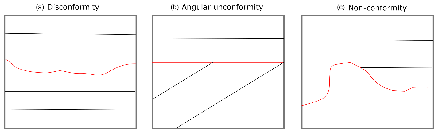
Figure 2 Unconformities interfaces (red lines) and geological interfaces (black lines) represent a break in depositional history. There are different possible geometries that an unconformity can have: (a) disconformity contact between two stratigraphic packages that share a similar geometry, (b) an angular unconformity where the younger stratigraphic package defines the geometry of the unconformity and (c) a nonconformity where the older stratigraphic package defines the geometry of the unconformity.

An unconformity is a geological interface where the rock units on either side are of significantly different ages, usually representing a period of erosion. In Fig. 3 the three conventional types of unconformity are shown. In Fig. 3a. the unconformity between the units is a disconformity and the geometry of the disconformity is not associated with either stratigraphic package. The disconformity is usually identified by the significant gap between the ages of the rocks. In this type of contact the layers actually share a similar geometry and for the purpose of 3D modelling the units could be represented by a single stratigraphic group. Angular unconformities (Fig. 3b) are observed when erosion occurs after some deformation (the older beds are not horizontal anymore) and before the next deposition of sedimentary layers. As the name suggests the angular unconformity represents a boundary between two differently oriented stratigraphic sequences. In a 3D model an angular unconformity can be introduced by setting the boundary between the two sequences to be the base of the younger package. In practice, this means that the two groups are modelled with two separate scalar fields. In Fig. 3c a nonconformity is shown; in this type of unconformity the geometry of the older unit defines the base of the younger unit. This could occur when a stratigraphic package is deposited on top of a crystalline basement.

2.2.2 Structural frames

A structural frame (Fig. 4) is a local coordinate system that is built around the major structural elements of a geological event. In LoopStructural structural frames are used for characterising the geometry of folds where the major structural element is the fold axial foliation (Fig. 4b) and the structural direction is roughly the fold axis. A fault frame is a structural frame where the major structural feature is the fault surface, the structural direction is the fault slip and the intermediate direction is the fault extent (Fig. 4). In LoopStructural, structural frames are built by first building the major structural feature which will typically have more observations, e.g. fault surface location or axial foliations. The structural direction is then built using any available observations of the structural direction, e.g. local observations of the fault slip or the fold axis, combined with an additional constraint which sets the gradient of the scalar field to be orthogonal to the major structural feature. The third coordinate can be built with an arbitrary value constraint, or value constraints to specify the extent of the field in this direction (e.g. for faults −1 and 1 specify the edges of the fault). This value constraint is combined with two global orthogonality constraints specifying that the scalar field should be orthogonal to both the major structural feature and the structural direction.

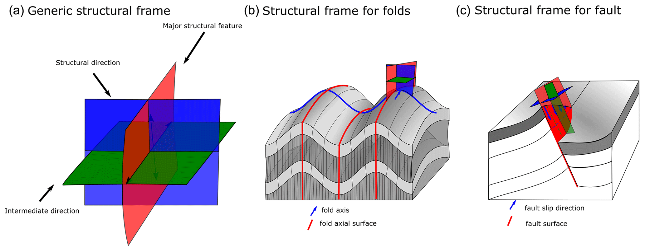
Figure 3 (a) Generic structural frame showing isosurfaces for three coordinates. (b) Structural frame for characterising a fold. (c) Structural frame for characterising fault geometry.

2.2.3 Faults

“A fault is a tabular volume of rock consisting of a central slip surface or core, formed by an intense shearing, and a surrounding volume of rock that has been affected by more gentle brittle deformation spatially and genetically related to the fault” (Fossen, 2010).

When adding faults there are two aspects to modelling the fault: (1) building the fault surface geometry and (2) integrating the fault displacement into older surfaces. Where possible, measurements of faults include the movement direction and the magnitude of displacement. There are three broad approaches for integrating faults into the implicit modelling framework: (1) add the fault into the implicit description of the surface (Calcagno et al., 2008a; de la Varga et al., 2019); (2) apply the fault after interpolating a continuous surface (Godefroy et al., 2018a; Laurent et al., 2013) and (3) represent the foot wall and hanging wall by separate implicit functions. Regardless of the approach used, the geometry of the fault surface is defined before defining the geometry of the surfaces displaced by the fault. The fault surface can be interpolated by building a scalar field where the fault surface is represented by an isovalue.

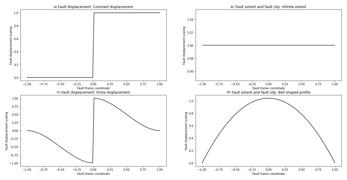
Figure 4 Fault displacement profiles: (a) constant displacement profile, (b) infinite-extent fault displacement showing no change in fault displacement along the fault extent or in the slip direction, (c) finite-extent fault displacement showing fault displacement decreasing with distance away from the fault, (d) finite-extent fault bell shaped profile for characterising fault displacement along the fault extent or in the slip direction.

In LoopStructural there are two ways of representing faults: (1) the fault kinematics are added into the implicit description of the scalar field of the faults and applied to the affected scalar field(s) (Grose et al., 2021a) and (2) faults are treated as domain boundaries and separate scalar fields are used to model the hanging wall and footwall of the fault. The kinematics of the fault are added into the implicit description of the faulted surface. To do this a fault frame is built (Fig. 4c) where three coordinates are interpolated: (1) a scalar field representing the distance to the fault surface, (2) a scalar field representing the distance along the slip direction of the fault and (3) a scalar field representing the extent of the fault. These coordinates can then be used to define the fault ellipsoid, which is a volumetric representation of the area deformed by the fault. The displacement of the fault can be defined relative to this coordinate system, e.g. the displacement of the fault should decay away from the fault centre along the fault extent and along the direction of displacement using the bell-shaped curve (Fig. 5d). The displacement may decrease with distance away from the fault centre perpendicular to the fault surface; this can be defined using the profile in Fig. 5c. If the displacement is constant within the model area the curves in Fig. 5a and b can be substituted for Fig. 5c and d respectively. The displacement curves shown in Fig. 5 can be substituted for any function of the fault frame coordinates. The same approach for combining the fault profiles (Fig. 5) within the fault frame has been used to define a volumetric fault displacement field (Jessell and Valenta, 1996; Godefroy et al., 2018b), the latter of which was adapted from the following Laurent et al. (2013):

$$\begin{array}{}\text{(6)}& \mathit{\delta }\left(x\right)=D_{\mathrm{0}}\left(f_{\mathrm{0}\left(X\right)}\right)\cdot D_{\mathrm{1}}\left(f_{\mathrm{1}}\left(X\right)\right)\cdot D_{\mathrm{2}}\left(f_{\mathrm{2}}\left(X\right)\right),\end{array}$$

where $D_{\mathrm{0},\mathrm{1},\mathrm{2}}$ are 1-D curves (e.g. any of the curves in Fig. 5) describing the displacement of the fault within the fault frame.

The fault frame can be built using a discrete implicit modelling approach as additional constraints can be added into the interpolation to enforce the orthogonality of the three coordinate systems. This is added into the interpolation matrix by adding a constraint for every element in the mesh where $\mathrm{\nabla }{\mathit{\varphi }}_{\mathrm{0}}\left(x,y,z\right)\cdot \mathrm{\nabla }{\mathit{\varphi }}_{\mathrm{1}}\left(x,y,z\right)=\mathrm{0}$. This constraint can be added twice so that when modelling ϕ₂ both ϕ₀ and ϕ₁ are orthogonal. In general, this means that if the fault orientation, fault trace and fault slip direction are known, the fault can be modelled. Where the fault slip is unknown, this can be substituted by conceptual knowledge, e.g. enforcing strike-slip faults or reverse faults.

2.2.4 Folds

Folds are challenging to model using classical implicit interpolation algorithms, because by definition a folded surface has a symmetry only defined by their axial surface. The symmetry is hard to reproduce by only interpolating orientations of the folded foliation as this would require orientations to be sampled in a symmetrical way across the axial surface (Laurent et al., 2016; Lisle et al., 2007; Mynatt et al., 2007). The regularisation of implicit algorithms are usually defined to minimise some sort of curvature between observations such as constant gradient regularisation, minimising second derivatives using finite differences or the weighted combination of infinite basis functions (Calcagno et al., 2008a; Cowan et al., 2003; Frank et al., 2007; Jessell et al., 2014; Lajaunie et al., 1997; Laurent, 2016; Mallet, 2014). As a result, to model folded geometries the geologist is required to add interpretive constraints such as synthetic bore holes, cross sections or simply synthetic constraints to produce model geometries that fit the geologist's conceptual idea of the fold (Caumon et al., 2003; Jessell et al., 2014, 2010).

There have been a number of different approaches to incorporating folds into implicit modelling including incorporating the fold axial surfaces (Laurent et al., 2016; Maxelon et al., 2009), the fold axis (Hillier et al., 2014; Laurent et al., 2016; Massiot and Caumon, 2010), both these structural elements and fold overprinting relationships (Laurent et al., 2016).

LoopStructural implements the following fold constraints: the fold axis, fold axial surface and overprinting relationships (Laurent et al., 2016) by adding additional constraints into a discrete interpolation approach. A fold frame (Figs. 4b and 6) is built where the principal axes of the fold frame correspond with the direction of the finite-strain ellipsoid. The fold frame allows for the geometry of the folded surface to be defined.

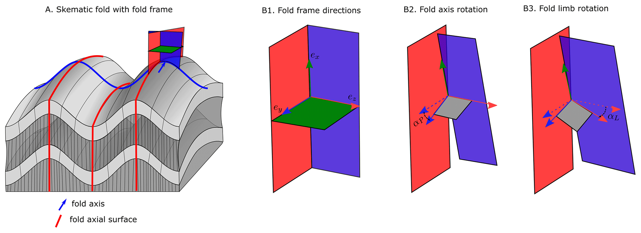
Figure 5 Schematic diagram of a fold adapted from Laurent et al. (2016) showing (a) fold frame, (b1) fold frame direction vectors, (b2) fold axis defined by fold axis rotation angle, (b3) folded foliation defined by fold limb rotation around fold axis.

The orientation of the fold axis (${\mathbf{F}}_{\mathrm{A}}^{\mathrm{T}}$) can be defined within the fold frame by rotating the fold axis direction field by the fold axis rotation angle (Fig. 6b2). The fold direction (${\mathbf{F}}_{\mathrm{D}}^{\mathrm{T}}$) is defined by rotating the normal to the axial foliation around the fold axis by the fold limb rotation angle. The orientation of the folded surface is the plane defined by the fold axis vector and the fold direction vector (Fig. 6b3). The fold constraints have been implemented into the piecewise linear interpolator using four main constraints, where φ(xyz) represents the implicit function, ∇ represents the gradient, t represents a tetrahedron where the constraint is applied and T1 and T2 are two tetrahedrons that share a face, and h_s is the expected magnitude of the gradient norm:

• The folded surface should contain the orientation of the fold axis: ${\mathbf{F}}_{\mathrm{A}}^{\mathrm{T}}\cdot \mathrm{\nabla }\mathit{\phi }\left(xyz\right)=\mathrm{0}$.

• The folded surface will contain the fold direction (solid red arrow in Fig. 6b3) vector: ${\mathbf{F}}_{\mathrm{D}}^{\mathrm{T}}\cdot \mathrm{\nabla }\mathit{\phi }\left(xyz\right)=\mathrm{0}$.

• The regularisation should only occur within the intermediate structural direction (e_x) ${\mathbf{e}}_{x\mathrm{0}}^{\mathrm{t}}\cdot \mathrm{\nabla }{\mathit{\phi }}_{\mathrm{T}\mathrm{1}}\left(xyz\right)-{\mathbf{e}}_{x\mathrm{1}}^{\mathrm{t}}\cdot \mathrm{\nabla }{\mathit{\phi }}_{\mathrm{T}\mathrm{2}}\left(xyz\right)=\mathrm{0}$.

• A similar fold constraint is as follows: ${\mathbf{e}}_x^{\mathrm{t}}\cdot \mathrm{\nabla }\mathit{\phi }\left(xyz\right)=\frac{\mathrm{1}}{h_{\mathrm{s}}}$.

The fold constraints require two angles to be known throughout the model: the fold axis rotation angle (α_P) and the fold limb rotation angle (α_L). The fold axis rotation angle (α_P) is the angle between the fold axis and e_y (Grose et al., 2017).

The fold limb rotation angle (α_L) is the angle that defines the orientation of the folded foliation relative to fold axial foliation and will be 0 in the hinge of the fold and positive and negative in the limbs (Grose et al., 2017). Grose et al. (2017) used the fold frame to calculate these angles for observations and then applied interpolation either using radial basis functions or by fitting an objective function (a Fourier series) to the rotation angles within the fold frame coordinates. The wavelength of the fold can be estimated by calculating an experimental semi-variogram of the fold rotation angle in the fold frame coordinates. For periodic folding, the experimental variogram has a periodic curve where the first peak indicates the half-wavelength of the fold (Grose et al., 2017).

In LoopStructural the default approach for fitting the fold rotation angle is to fit a Fourier series. The fold axis rotation angle is calculated first; the wavelength is first estimated automatically using the gradient descent method on the experimental variogram of the fold axis. The fold rotation angle is optimised using the scipy.optimize.curve_fit method using non-linear least squares to fit wavelength and Fourier coefficients. The fold axis can then be defined throughout the model by applying the rotation of e_y⋅R_p. If the fold axis is constant (cylindrical folding), a constant fold axis vector can be used.

The fold limb rotation angle is calculated by finding the complementary angle between the normal to the folded foliation and e_z in the plane perpendicular to the fold axis. The fold limb rotation angle can be interpolated by fitting a Fourier series to the observations in the same way as fitting the fold axis rotation angle.

Grose et al. (2018, 2019) use inverse problem theory to fit a forward model of the fold geometry to the observed fold rotation angles. The joint posterior distribution of the fold parameters (Fourier series coefficients, fold wavelength and a misfit parameter) are sampled using Bayesian inference. This allows multiple fold geometries to be explored without perturbing the datasets. LoopStructural does not provide a direct probabilistic interface; however, it is possible to define a probabilistic representation of the fold geometry curves and add this into the modelling workflow. An example using the Python library emcee (Foreman-Mackey et al., 2013) is provided in the LoopStructural documentation.

3 Implementation in LoopStructural

3.1 Loop structural design

LoopStructural is written using Python 3.6+, using numpy data structures and operations. The design of LoopStructural follows an object-oriented architecture with multiple levels of inheritance. Object-oriented design allows for LoopStructural to be used as a development platform for 3D geological modelling, where new features can be added without needing to implement boiler plate code. There are five submodules that can be imported into a Python environment:

1. core contains the core modelling functionalities and the management of the geological concepts.

2. interpolation contains the various interpolation code and supports used to build scalar fields.

3. datasets contains the test and reference datasets.

4. utils contains miscellaneous functions.

5. visualisation contains model visualisation tools.

The creation and management of different geological objects is managed by the GeologicalModel. To initialise an instance, the required arguments are the minimum and maximum extents of the bounding box, which are specified by two separate vectors. The default behaviour is to define a rescaling coefficient as follows:

$$\begin{array}{}\text{(7)}& \text{scale}=\max (x_{\max }-x_{\min },y_{\max }-y_{\min }{z}_{\max }-z_{\min }).\end{array}$$

Adding different geological objects can be done through using an instance of GeologicalModel. There are four different types of observations that can be incorporated into an interpolation algorithm:

1. value constrains the value of the scalar field at a particular location and can either represent the location of a surface or the distance away from the surface.

2. gradient constrains only the gradient of the scalar field; e.g. the normal to the scalar field should be orthogonal to two vectors within the gradient plane.

3. tangent is the scalar field and should be orthogonal to a vector.

4. norm constrains the direction and magnitude of the scalar field norm.

The data can be associated with the GeologicalModel using the set_data(data) method where “data” is a pandas data frame. When added into the model the data points are transformed into the model coordinate system.

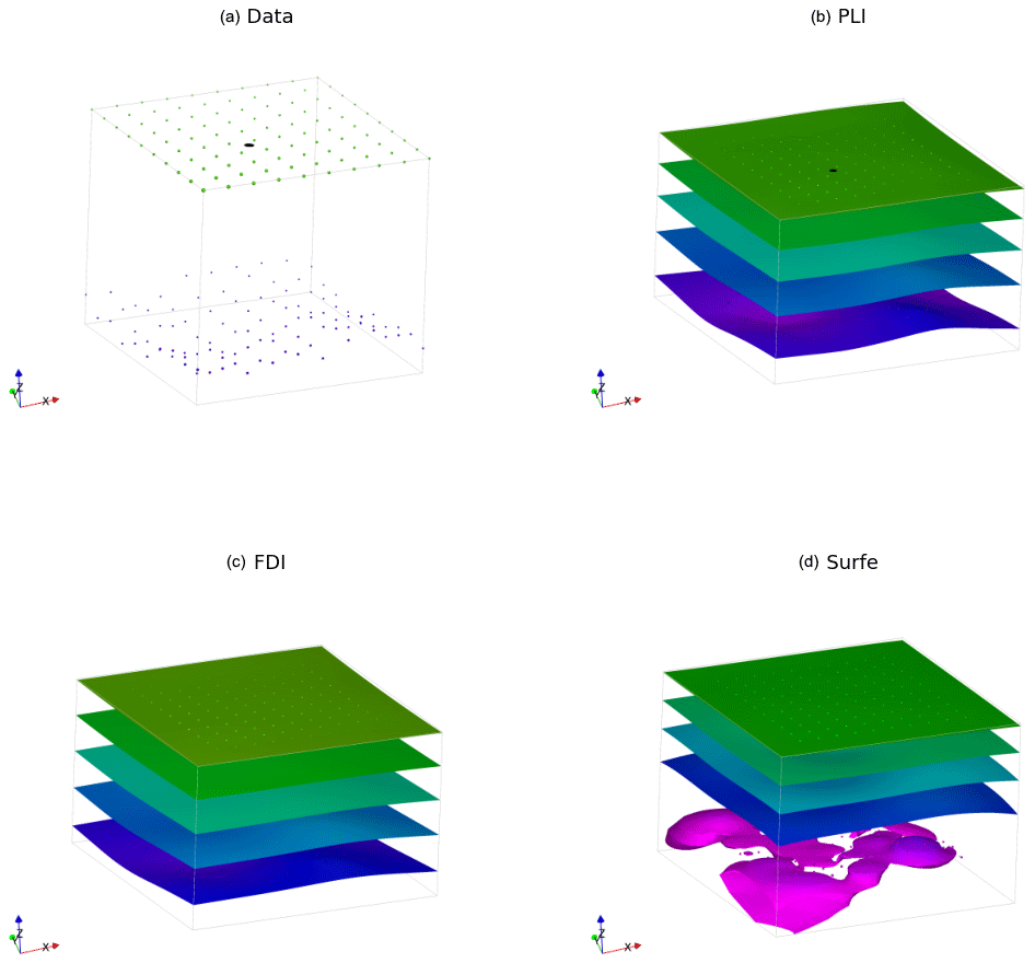
Figure 6 Comparison of interpolation methods for synthetic surfaces where two isosurfaces are shown coloured by the local z coordinate: (a) input data, (b) surfaces interpolated using PLI, (c) surfaces interpolated using FDI, (d) surfaces interpolated using SurfE; note the lower isosurface has a non-manifold geometry.

3.2 Adding geological objects

Within LoopStructural geological objects such as stratigraphy, faults, folding event and unconformities are all represented by a GeologicalFeature. A GeologicalFeature can be evaluated for the value of the scalar field and/or the gradient of the scalar field at a location.

The GeologicalModel contains an ordered collection of geological features and determines how the features interact. For example, unconformity geological features act as a mask to determine where the interface between packages should be. The ordering of the GeologicalFeatures inside the model reflects the timing of the geological events being modelled. The most recent features are added first as their geometry is used to constrain the older features.

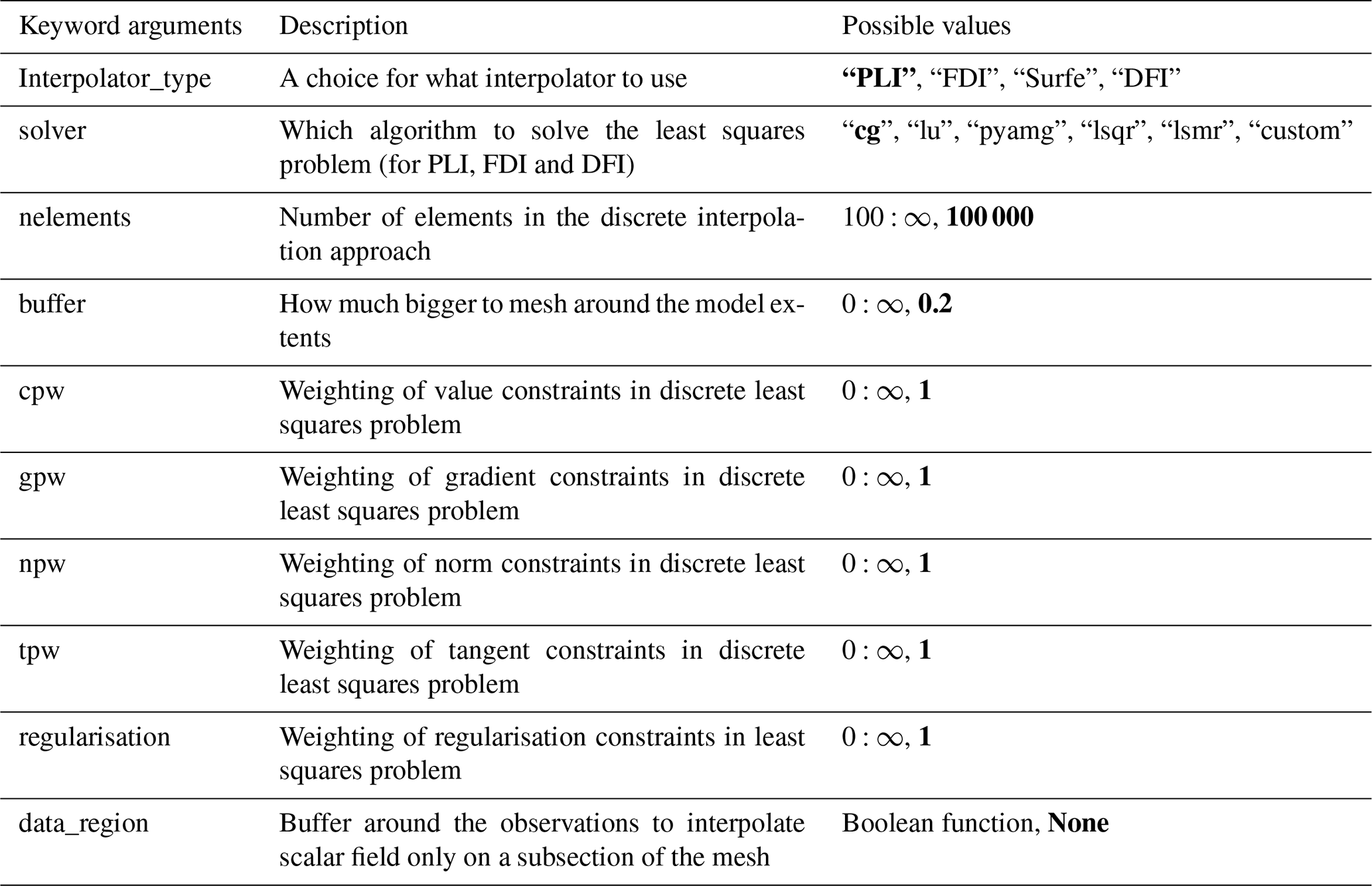
There are different ways a GeologicalFeature can be added to a GeologicalModel depending on the type of geological object that is being modelled. The LoopStructural GeologicalModel class provides an interface for creating geological objects, where different types of geological features can be added using different functions. All geological objects are represented by one or multiple volumetric scalar field. These scalar fields can be built using an implicit interpolation algorithm where the implicit function is approximated from observations of the scalar field. Alternatively, a GeologicalFeature can be represented by an analytical function (or a combination of existing GeologicalFeatures). LoopStructural allows for different interpolation algorithms to be specified for different GeologicalFeatures within the same model. The interpolation algorithm and any parameter definitions are specified by adding additional keyword arguments to the function. Table 1 outlines the possible arguments that can be specified for the interpolator.

Table 1 Interpolation keyword arguments. Default values are highlighted by bold text.

3.3 Model output

LoopStructural includes a number of helper functions for evaluating the GeologicalModel on an array of coordinates within the model. The following functions can be called from a GeologicalModel as shown in the code below.

• To evaluate the lithology value at a location the function evaluate_model(xyz) returns a numpy array containing the integer ID of the stratigraphy that was specified in the stratigraphic column.

• To evaluate the value of a GeologicalFeature at a location within the model the function evaluate_feature_value(feature_name,xyz) returns the value of the scalar field that represents the geological feature.

• To evaluate the gradient of a GeologicalFeature the evaluate_feature_gradient(feature_name,xyz) can be called.

Triangulated surfaces can be extracted from a GeologicalFeature within LoopStructural and exported into common mesh formats, e.g. Visualisation ToolKit (.vtk) or Wavefront (.obj). These surfaces can then be imported into external software, e.g. ParaView⁵.

3.4 Model visualisation

LoopStructural has three different visualisation tools that can be accessed from the LoopStructural.visualisation module:

1. LavaVuModelViewer. LavaVu (Kaluza et al., 2020) is a visualisation module that provides interactive visualisation. We use LavaVu for visualising triangulated surfaces representing the geological interfaces as well as the scalar field representing the implicit function. The creation and manipulation of LavaVu objects is wrapped by the LavaVuModelViewer class which provides an interface to the GeologicalModel. This is an interactive (and static) 3D visualisation using LavaVu.

2. MapView. This is a 2D visualisation (cross section, map) using matplotlib (Hunter, 2007) that can create a geological map from the resulting geological model. Input datasets can be plotted drawing the location of contacts and the orientation of the contacts using the strike and dip symbology. The scalar field can be evaluated on the map surface, contours can be drawn or the geological model can be plotted onto the map.

3. FoldRotationAnglePlotter. This is a visualisation module for producing S plots and S-variogram plots for a folded geological feature. Plotting is handled using matplotlib.

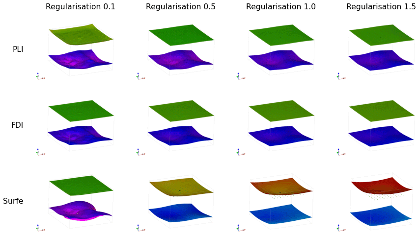
Figure 7 Implicit surfaces calculated for regularisation constraints (0.1,0.5,1,1.5) using piecewise linear interpolator (PLI), finite-difference interpolator (FDI) and radial basis function (SurfE).

4 Examples

4.1 Implicit surface modelling

In the first example we will demonstrate modelling two synthetic surfaces using the same scalar field within a model volume of ($-\mathrm{0.1},-\mathrm{0.1},-\mathrm{0.1}$) and $\left(\mathrm{5.1},\mathrm{5.1},\mathrm{5.1}\right)$. The observations are two sets of points. The first set forms a surface at points on a regular grid for z=4 and the second set forms a surface at $z=\mathrm{0.2}\cdot \sin \left(x\cdot \mathrm{10}\right)+\mathrm{0.2}\cdot \cos \left(y\right)+\mathrm{0.15}\cdot N\left(\mathrm{0},\mathrm{0.1}\right)$ where N(0,0.1) is a normal distribution with a mean of 0 and standard deviation of 0.1.

In Fig. 7a the data points are shown, and in Fig. 7b, c and d the same surfaces are interpolated using the three default interpolation algorithms in LoopStructural (PLI – piecewise linear interpolator, FDI – finite-difference interpolator and SurfE – radial basis interpolation). The results for the interpolation using PLI and FDI are very similar, as both interpolation algorithms use least squares to fit observations whilst minimising a global regularisation term that effectively minimises the second derivative of the implicit function. This means that the interpolant balances fitting the observations with minimising the roughness of the resulting surfaces. The radial basis interpolation used by SurfE is a direct interpolation approach, which means that the interpolant must fit all of the observations (although a smoothing constraint can be used). In this example, because the surfaces are over-constrained to a highly variable point set the resulting surface is non-manifold (cannot be unfolded into a flat plane). While this does not necessarily mean the surface is incorrect it is geologically unlikely.

The weighting of the regularisation constraint generally has the biggest impact on the resulting geometry when using the discrete interpolation approaches. In Fig. 8 the regularisation constraint is varied from 0.1 (rougher surface) to 1.5 (smoother surface). Lower regularisation constraints result in surfaces that more closely fit the observations at the cost of a more irregular surface. However, even for the lowest regularisation constraints the surfaces still do not fit every observation. There is no explicit rule for choosing the relative weighting of the regularisation, as it is often dependent on the surfaces being modelled. For example, when modelling a surface where the underlying process causing the variation in the data points is non-stationary, a higher regularisation constraint is appealing as the goal of the modelling is to reproduce the effect of this process. However, if the perturbations are the result of a process we are trying to model (probably a stationary process) then a lower regularisation constraint would be appealing. A smoothing constraint can be added into the radial basis interpolation which aims to increase the smoothness of the resulting surface. The smoothing constraint for data-supported methods adds a buffer to how closely the function must fit the observations. In Fig. 8 increasing regularisation results in smoother surfaces; however, with this approach the fit to both surfaces is impacted, which can be seen by the change in colour of the surface, which represents the local height of the surface.

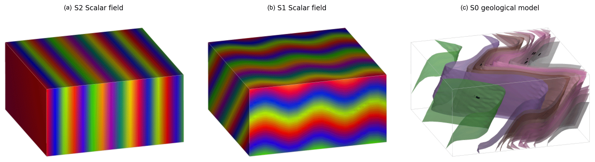
Figure 8 Structural data for refolded fold: (a) observations of S2, (b) observations of S1 showing interpolated scalar field of S2 and (c) observations of S0 showing interpolated scalar field of S1.

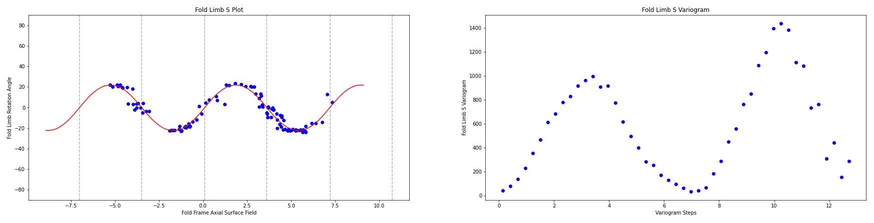
Figure 9 F2 S plot showing the fold rotation angle between observations of S1 and the fold frame S2.

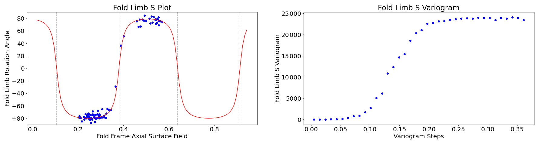
Figure 10 F1 S plot showing the fold rotation angle between observations of S0 and the fold frame S1.

Figure 11 Scalar fields: (a) S2, (b) S1 and (c) bedding.

4.2 Modelling folds: type 3 interference

To demonstrate the time-aware approach for modelling folds we reuse the case study from Laurent et al. (2016). The reference model was generated using Noddy (Jessell and Valenta, 1996) with two folding events forming a type 3 interference pattern:

1. F1 involves large-scale recumbent folding (wavelength: 608 m, amplitude: 435 m, fold axis: N000E/45^∘).

2. F2 involves upright open folding (wavelength: 400 m, amplitude: 30 m).

The structural observations were sampled from a synthetic topographical horizon from three outcrop locations. The axial foliation to F2, S2, is shown in Fig. 9a. The observations of S2 are used to interpolate the major structural feature of the F2 fold frame (Fig. 12a). The axial foliation of F1, S1, is shown in Fig. 9b, and the scalar field value of the interpolated S2 is shown on the map. The fold rotation angle for F2 is calculated by finding the angle between the interpolated S2 field and the folded S1 field and is shown in the S plot for Fig. 10a. The red curve in Fig. 10a is a Fourier series that is automatically fitted to the observations. The wavelength of the fold is estimated by finding the first peak of the S variogram (Fig. 10b). Fold constraints are added into the interpolation algorithm using this curve to define the geometry of the fold along the fold axis, and the average intersection lineation between the S1 foliation and the interpolated S2 field is a proxy for the fold axis. The interpolated scalar field is shown in Fig. 12b. The observations of S0 are shown in Fig. 9c, and the scalar value of the S1 field is shown on the map. The S plot for F1 is shown in Fig. 11a and shows two opposing fold limbs in the data points. The red curve shows the Fourier series that characterises the geometry of the fold along the fold axis and indicates that there are two unobserved fold hinges away from the data points. These constraints are added into the implicit model, and the scalar field is shown in Fig. 12c.

4.3 Integration with map2loop

In the final examples we use map2loop (Jessell et al., 2021) as a pre-processor to generate an input dataset from regional geological survey maps, the national stratigraphic database and a global digital elevation model. map2loop creates a set of augmented data files that can be used to build a geological model in LoopStructural. The class method (GeologicalModel.from_map2loop_directory(m2l_directory, **kwargs)) creates an instance of a GeologicalModel from a root map2loop output directory. We will demonstrate the interface between map2loop and LoopStructural with two case studies (1) from the Flinders Ranges in South Australia and (2) from the Hamersley region in Western Australia. The first case study demonstrates the interface between map2loop and LoopStructural for a large regional model. The second case study shows how the conceptual model used to generate the input dataset can be varied.

The first example uses a small study area from South Australia using the Geological Survey of South Australia's open-access datasets (GSSA, 2020). The model area covers approximately 85 km by 53 km within the Finders Ranges in South Australia. The stratigraphic units within this area are shown in Fig. 13a, and the outcropping geology is shown in the geological map (Fig. 13b); the patches of the map without any geological units represent shallow Tertiary and Quaternary cover. map2loop extracts basal contacts from the outcropping geological units and estimates the layer thicknesses shown in the stratigraphic column. Within this map area all of the stratigraphic groups share a similar deformation history and area modelled as a single super-group. The cumulative thickness is estimated for all of the stratigraphic horizons relative to the Pound Subgroup and is used to constrain the value of the implicit function. There are 15 faults within the model area with limited geometrical information constraining only the map trace of the faults. As a result, the faults are assumed to be vertical with a vertical slip direction, and the displacements are estimated from the geometry on the geological map using map2loop. The geometry of the fault can be changed within LoopStructural and map2loop to explore the uncertainty space. The overprinting relationships of the faults are estimated from the geological map using map2loop by analysing the intersection between faults on the geological map. The estimated overprinting relationships are used to constrain the order of the faults in the geological model. The scalar field representing the supergroup is interpolated after the observations of the stratigraphic horizon (contacts and orientation measurements) are un-faulted using the calculated fault displacements. The modelling workflow is all encapsulated in the (GeologicalModel.from_map2loop_directory(m2l_directory, **kwargs)) class method, meaning the geological model can be produced without any user input.

The resulting geological model surfaces are shown in Fig. 14 where the surface represents the base of a stratigraphic group and are coloured using the stratigraphic column (Fig. 13a). The faults in the model are interpolated using a Cartesian grid with 50 000 elements and are interpolated using the finite-difference interpolator, and the interpolation matrix is solved using the pyamg algorithmic multigrid solver (Olson and Schroder, 2018). Stratigraphy is interpolated using a finer mesh with 500 000 elements using the finite-difference interpolator and also using pyamg. Using a workstation laptop with an i7 processor and 32gb of RAM the data processing using map2loop takes approximately 1 min, building the implicit model takes approximately 8 min and the rendering of the surfaces on a ($\mathrm{200}\times \mathrm{200}\times \mathrm{100}$) Cartesian grid takes 3 min. The intersection of the solid geological model and the map surface is shown in Fig. 13c, allowing for a comparison with the input dataset. The geological model has interpolated the geological packages underneath the surficial deposits.

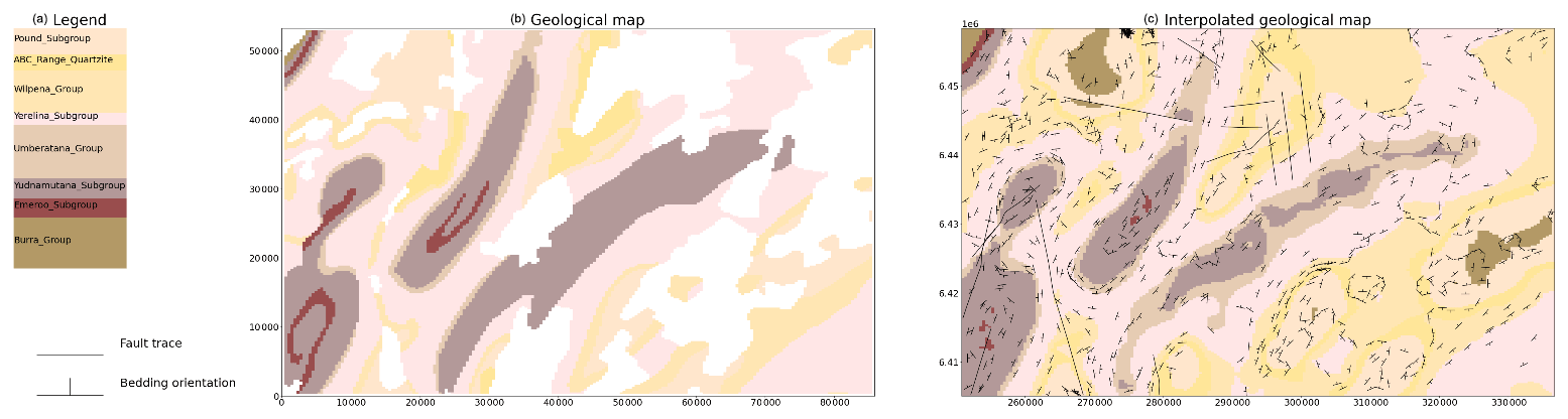
Figure 12 (a) Stratigraphic column for model area showing relative thickness. (b) Geological map showing bedding and faults. (c) Geological model shown on map surface.

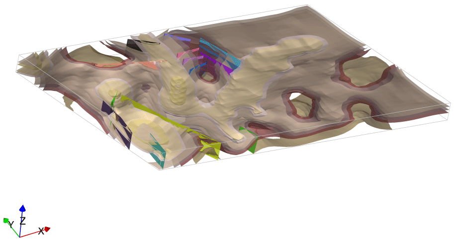
Figure 13 Geological model from South Australia using map2loop processed data stratigraphic surfaces using colours from Fig. 12a and fault surfaces.

In the second example we use map2loop to process a small area of the Turner Syncline in the Hamersley region in Western Australia using data provided by the Geological Survey of Western Australia (GSWA) (2016). The model area is 12 km × 13 km and includes three faults. The default assumption by map2loop is that the faults are vertical and are purely dip slip, and the hanging wall and displacement are estimated by analysing the map pattern of the faulted units (for more information about this process the reader is referred to Jessell et al., 2021). In this example, we have created 12 realisations of the geological model by rotating the fault slip direction from a vertical vector around the normal to the fault surface. The resulting models are shown in Fig. 14 where the fault slip vector is shown as a pole on the stereonet and the fault plane is shown by a great circle. The results show a wide range in geometries with some structures being unlikely, for example a rotation of 120^∘ removes the map expression of the western fault. LoopStructural provides an easy interface to allow for the kinematics and conceptual models for different geological features to be incorporated into the modelling workflow.

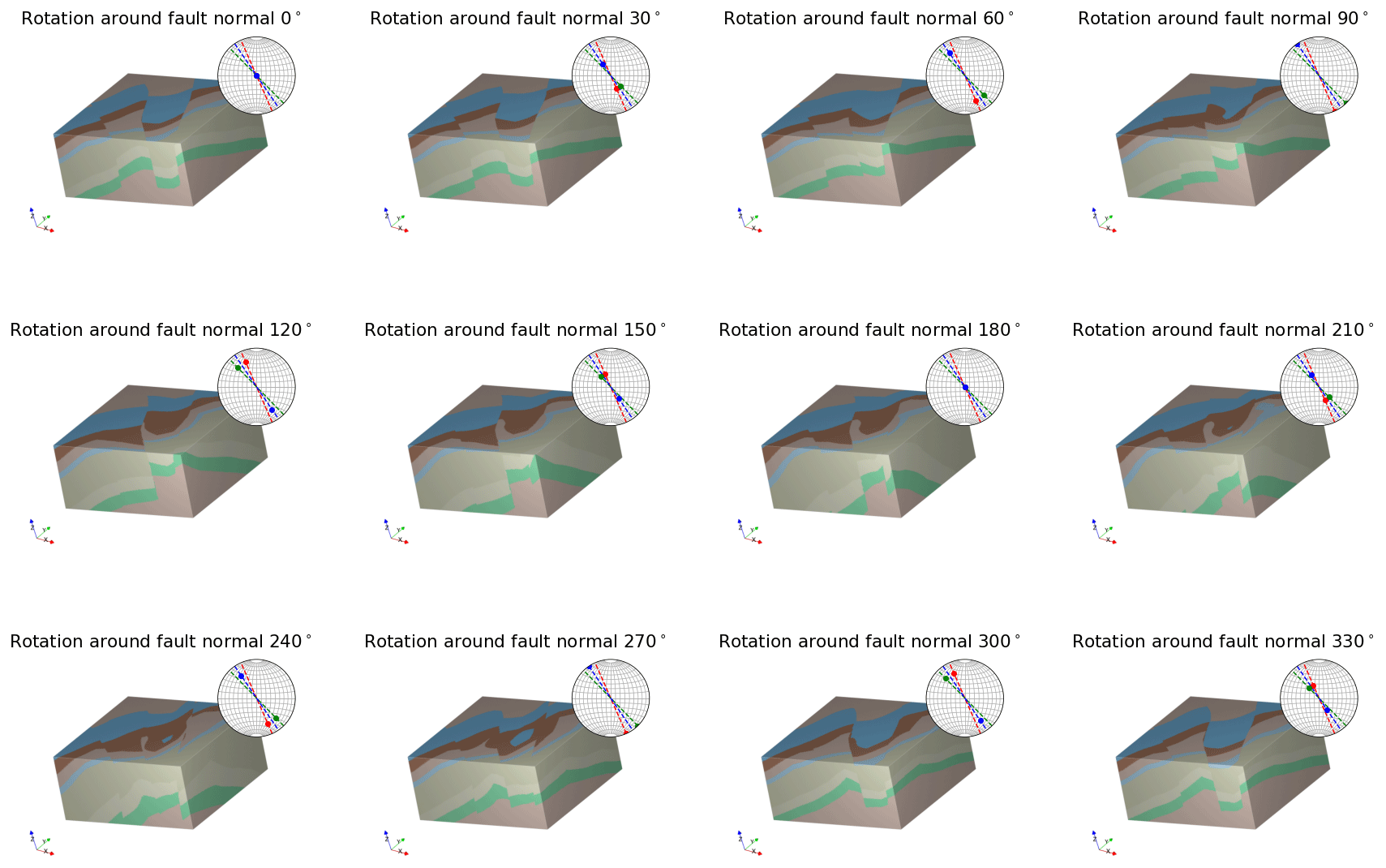
Figure 14 The 12 model iterations where initial fault slip vector has been rotated around the normal to the fault surface. Stereonets show the resulting fault slip vectors (poles) and the fault plane (great circles).

5 Discussion

LoopStructural is the 3D geological modelling module for Loop, a new open-source 3D probabilistic geological and geophysical modelling platform. LoopStructural integrates the relative timing of geological features into the description of the model elements using a time-aware modelling approach where the model is built by adding geological features in the reverse order from which they occur. This is necessary for capturing the complexities of complex structural geometries, for this approach is used for modelling refolded folds (Fig. 12). In a similar way faults are added backwards in time; this means that the displacements of the faults are applied to the model prior to interpolating the faulted surface. As a result, the fault displacements and overprinting relationships are internally consistent. In comparison, where faults are represented using step functions (Calcagno et al., 2008b; de la Varga and Wellmann, 2016) the fault displacements are added into the interpolation of the faulted surfaces using the polynomial trend in the dual co-kriging system, meaning the cumulative displacement is determined as the best global fit, rather than incorporating the displacements of individual faults.

LoopStructural provides a flexible open-source implementation of implicit geological modelling algorithms workflows. The motivation behind developing LoopStructural was to create a framework for being able to develop new implicit geological modelling algorithms and tools. LoopStructural has native implementation of piecewise linear interpolation (Caumon et al., 2013; Frank et al., 2007; Mallet, 1992, 2004), including the fold constraints (Grose et al., 2017; Laurent et al., 2016) and a finite-difference interpolator, minimising the second derivative as a regularisation constraint (Irakarama et al., 2018). In Fig. 8 we showed that choosing the regularisation weight is somewhat dependent on the quality of the input dataset. For this reason, varying the regularisation weight and interpolation approach should be a common step in implicit modelling workflows. The current implementation of the piecewise linear interpolation uses a tetrahedral mesh that is derived from a Cartesian grid. A more sophisticated mesh generated from an external mesh generation code could be integrated into LoopStructural by overwriting the tetrahedral mesh class with a custom class. Within the LoopStructural architecture alternative regularisation constraints could easily be incorporated. For example, it is possible to define custom constraints for implementation within the finite-difference scheme; the user simply has to provide a dictionary containing 3D numpy arrays, where each pixel in the array represents the 3D finite-difference mask and a relative weighting. New interpolation schemes can be easily implemented using various levels of inheritance to avoid re-writing boiler plate code. For example, the interface with SurfE capitalises on the object-oriented design of LoopStructural, where the interface between LoopStructural and SurfE was achieved by creating a new class which inherits the components for the base geological interpolation class. Both the piecewise linear interpolator and finite-difference interpolator inherit from a base discrete interpolation class which manages the assembly of the least squares system and the solving of the least squares problem. This object-oriented design allows for the interpolation algorithms to be interchanged and re-implemented without modifying the other aspects of the geological modelling.

A recent focus of 3D modelling research has been to simulate uncertainties by framing the problem as an inverse problem, where the data points are the parameters of the forward model (de la Varga et al., 2019). This allows for additional geological knowledge to be integrated into the model definition such as fault displacement, fault type and fold geometry. Within LoopStructural, we have directly integrated many aspects of the geological knowledge into the interpolation schemes and model definition. The fundamental reasoning behind our approach is that the subjective constraints that are required to capture the geological features with standard implicit algorithms will be one of the greatest sources of uncertainty in the model. By incorporating the geological concepts into the geological modelling algorithms, these conceptual uncertainties can be integrated into a probabilistic definition of the geological model. Currently, LoopStructural does not have a probabilistic interface; however, all parameters relating to geological structures (topological ordering, fold geometries, fault displacement and geometries) are accessible from the GeologicalModel class functions.

In Fig. 14, map2loop (Jessell et al., 2021) generates an augmented dataset from the open-access geological survey databases (stratigraphic database, DTM, geology shapefiles, structural lines and structural observations). In this example, the total time from data processing to model rendering was approximately 10 min. Using discrete implicit modelling means that the complexity of the model is defined by the resolution of the support, rather than the number of observations. Discrete interpolation involves solving the linear equation $\mathbf{A}\cdot x=\mathit{b}$ where A is a sparse matrix. Different algorithms can be used for solving this linear system. For example, the algorithmic multigrid solver used in the Flinders Ranges model can be substituted for the default conjugate gradient solver increasing the interpolation time. The algebraic solver uses multiple levels of conjugate gradient solvers for coarse grids to approximate the solution to the interpolation problem. The coarse grid solution is then used for improving the solving of the next level. Other approaches to speeding up the linear system could be applied such as using preconditioner for the conjugate gradient solver.

The fault displacement profiles (Fig. 5) define the fault displacement within the fault volume; however, these conceptual profiles are not fitted to the observations. Godefroy et al. (2018b) interpolate a continuous surface without observations within the fault domain and then use particle swarm optimisation to fit the displacement profiles to the unused observations. LoopStructural cannot apply this same approach because all data points are restored (with respect to the fault displacement) prior to interpolating the faulted surfaces. The displacement estimates calculated by map2loop could be used to estimate the displacement profile along the fault trace. The fault displacements could then be optimised using a probabilistic representation of the model geometry parameters. Within the same framework it would be necessary to include the parameterisation of the fault slip vector and fault dip if these are defined by a conceptual model rather than observations. However, defining a specific likelihood function for constraining the fault displacement is challenging and may be specific to the geology in question – e.g. where observations are abundant it would be possible to adopt the technique from Godefroy et al. (2018b) and separate some data from the interpolation; however, when dealing with typical regional scale map sheets most of the observations occur on the surface with limited constraints on the 3D geometry.

6 Conclusions

In this contribution we have introduced LoopStructural, a new open-source Python library for implicit 3D geological modelling. The key features of LoopStructural are as follows:

• implicit 3D geological modelling algorithms using discrete interpolation,

• implementation of structural geology of folds and faults using structural frames,

• a direct link to map2loop for automated 3D geological modelling,

• an object-oriented software design allowing for easy development and extension of the 3D modelling algorithms.

LoopStructural uses a time-aware modelling approach where relative timing between different geological features (folding, faulting and stratigraphy features) allows for complex overprinting relationships to be incorporated into the implicit geological models. Folds and faults are encoded using structural frames, a curvilinear coordinate system that is oriented with the geometry of the major structural feature of the deformational event. Using structural frames, the geometry of folds and faults can be locally characterised similarly to how a structural geologist describes the objects in the field.

Appendix A: Tetrahedral mesh

A cube is defined by eight vertices and can be referenced inside a Cartesian grid by the indices ijk. We subdivide each cubic element in a Cartesian grid into five tetrahedrons. To ensure that neighbouring tetrahedrons share common faces two masks need to be applied. We apply the even mask when $i+j+k$ is even.

Figure A1 Odd and even masks for extracting tetrahedrons from a Cartesian grid.

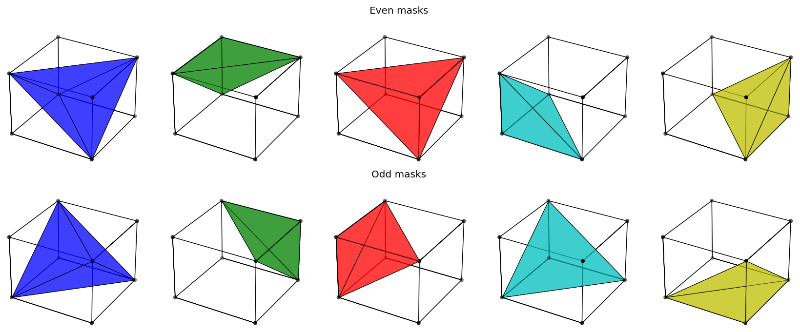
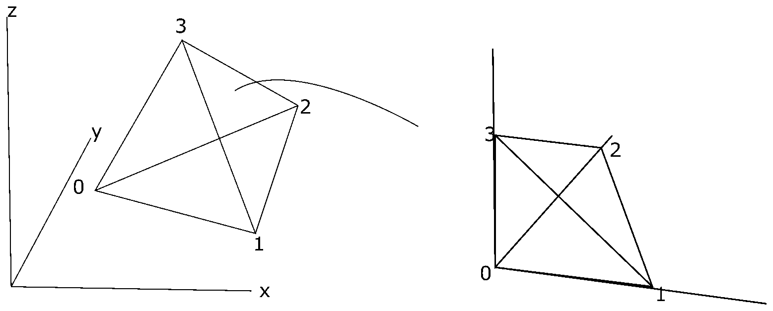
Figure A2 Schematic diagram showing transformation from tetrahedron in Cartesian space to reference tetrahedron in natural coordinates. This transformation allows for the shape functions and derivatives to be simplified.

The property is interpolated linearly within the element,

$$\begin{array}{}\text{(A1)}& \mathit{\varphi }\left(x,y,z\right)=a+bx+cy+dz.\end{array}$$

This can be expressed by the values at the nodes (0–3):

$$\begin{array}{}\text{(A2)}& {\displaystyle }{\mathit{\varphi }}_{\mathrm{0}}=a+b{x}_{\mathrm{0}}+c{y}_{\mathrm{0}}+d{z}_{\mathrm{0}},\text{(A3)}& {\displaystyle }{\mathit{\varphi }}_{\mathrm{1}}=a+b{x}_{\mathrm{1}}+c{y}_{\mathrm{1}}+d{z}_{\mathrm{1}},\text{(A4)}& {\displaystyle }{\mathit{\varphi }}_{\mathrm{2}}=a+b{x}_{\mathrm{2}}+c{y}_{\mathrm{2}}+d{z}_{\mathrm{2}},\text{(A5)}& {\displaystyle }{\mathit{\varphi }}_{\mathrm{3}}=a+b{x}_{\mathrm{3}}+c{y}_{\mathrm{3}}+d{z}_{\mathrm{3}}.\end{array}$$

Solving this set of linear equations for a, b, c, d depends on the location of the tetrahedron nodes and has to be recalculated for every tetrahedron. This can be simplified by applying a coordinate transformation to a reference tetrahedron (Fig. 2). This simplifies the solution and allows for the interpolation to be described by the barycentric coordinates (c₀c₁c₂c₃) of the tetrahedron. The barycentric coordinates can be used as a local coordinate system for the tetrahedron (ξηζ).

Since

$$\begin{array}{}\text{(A6)}& {\displaystyle }{c}_{\mathrm{0}}+c_{\mathrm{1}}+c_{\mathrm{2}}+c_{\mathrm{3}}=\mathrm{1},\text{(A7)}& {\displaystyle }\mathit{\xi }=c_{\mathrm{1}},\text{(A8)}& {\displaystyle }\mathit{\eta }=c_{\mathrm{2}},\text{(A9)}& {\displaystyle }\mathit{\zeta }=c_{\mathrm{3}}.\end{array}$$

The property within the tetrahedron can be interpolated using the four shape functions below:

$$\begin{array}{}\text{(A10)}& {\displaystyle }{N}_{\mathrm{0}}\left(\mathit{\xi },\mathit{\eta },\mathit{\zeta }\right)=\mathrm{1}-\mathit{\xi }-\mathit{\eta }-\mathit{\zeta },\text{(A11)}& {\displaystyle }{N}_{\mathrm{1}}\left(\mathit{\xi },\mathit{\eta },\mathit{\zeta }\right)=\mathit{\xi },\text{(A12)}& {\displaystyle }{N}_{\mathrm{2}}\left(\mathit{\xi },\mathit{\eta },\mathit{\zeta }\right)=\mathit{\eta },\text{(A13)}& {\displaystyle }{N}_{\mathrm{3}}\left(\mathit{\xi },\mathit{\eta },\mathit{\zeta }\right)=\mathit{\zeta }.\end{array}$$

The gradient of the function within the tetrahedron ∂ϕ_T can be found by applying the chain rule between the derivative of the shape function within the barycentric coordinates and the partial derivatives with respect to the natural coordinates and Cartesian coordinates:

$$\begin{array}{}\text{(A14)}& {\displaystyle }\begin{array}{rl}{\displaystyle \frac{\partial {\mathit{\phi }}_T}{\partial x}}& =\sum _{i=\mathrm{0}}^{\mathrm{3}}f\left(x_i,y_i,z_i\right)\\ & \cdot \left({\displaystyle \frac{\partial N_i}{\partial \mathit{\xi }}}{\displaystyle \frac{\partial \mathit{\xi }}{\partial x}}+{\displaystyle \frac{\partial N_i}{\partial \mathit{\eta }}}{\displaystyle \frac{\partial \mathit{\eta }}{\partial x}}+{\displaystyle \frac{\partial N_i}{\partial \mathit{\zeta }}}{\displaystyle \frac{\partial \mathit{\zeta }}{\partial x}}\right),\end{array}\text{(A15)}& {\displaystyle }\begin{array}{rl}{\displaystyle \frac{\partial {\mathit{\phi }}_T}{\partial y}}& =\sum _{i=\mathrm{0}}^{\mathrm{3}}f\left(x_i,y_i,z_i\right)\\ & \cdot \left({\displaystyle \frac{\partial N_i}{\partial \mathit{\xi }}}{\displaystyle \frac{\partial \mathit{\xi }}{\partial y}}+{\displaystyle \frac{\partial N_i}{\partial \mathit{\eta }}}{\displaystyle \frac{\partial \mathit{\eta }}{\partial y}}+{\displaystyle \frac{\partial N_i}{\partial \mathit{\zeta }}}{\displaystyle \frac{\partial \mathit{\zeta }}{\partial y}}\right),\end{array}\text{(A16)}& {\displaystyle }\begin{array}{rl}{\displaystyle \frac{\partial {\mathit{\phi }}_T}{\partial z}}& =\sum _{i=\mathrm{0}}^{\mathrm{3}}f\left(x_i,y_i,z_i\right)\\ & \cdot \left({\displaystyle \frac{\partial N_i}{\partial \mathit{\xi }}}{\displaystyle \frac{\partial \mathit{\xi }}{\partial z}}+{\displaystyle \frac{\partial N_i}{\partial \mathit{\eta }}}{\displaystyle \frac{\partial \mathit{\eta }}{\partial z}}+{\displaystyle \frac{\partial N_i}{\partial \mathit{\zeta }}}{\displaystyle \frac{\partial \mathit{\zeta }}{\partial z}}\right).\end{array}\end{array}$$

Appendix B: Trilinear interpolation in a cubic element

The implicit function can be described relative to the eight vertices of the cell using the shape functions ($N_{\mathrm{0},\mathrm{\dots },\mathrm{7}}$):

$$\begin{array}{}\text{(B1)}& {\displaystyle }{N}_{\mathrm{0}}={\displaystyle \frac{\mathrm{1}}{\mathrm{8}}}\left(\mathrm{1}-\mathit{\xi }\right)\left(\mathrm{1}-\mathit{\eta }\right)\left(\mathrm{1}-\mathit{\zeta }\right),\text{(B2)}& {\displaystyle }{N}_{\mathrm{1}}={\displaystyle \frac{\mathrm{1}}{\mathrm{8}}}\left(\mathrm{1}+\mathit{\xi }\right)\left(\mathrm{1}-\mathit{\eta }\right)\left(\mathrm{1}-\mathit{\zeta }\right),\text{(B3)}& {\displaystyle }{N}_{\mathrm{2}}={\displaystyle \frac{\mathrm{1}}{\mathrm{8}}}\left(\mathrm{1}+\mathit{\xi }\right)\left(\mathrm{1}+\mathit{\eta }\right)\left(\mathrm{1}-\mathit{\zeta }\right),\text{(B4)}& {\displaystyle }{N}_{\mathrm{3}}={\displaystyle \frac{\mathrm{1}}{\mathrm{8}}}\left(\mathrm{1}+\mathit{\xi }\right)\left(\mathrm{1}-\mathit{\eta }\right)\left(\mathrm{1}+\mathit{\zeta }\right),\text{(B5)}& {\displaystyle }{N}_{\mathrm{4}}={\displaystyle \frac{\mathrm{1}}{\mathrm{8}}}\left(\mathrm{1}-\mathit{\xi }\right)\left(\mathrm{1}-\mathit{\eta }\right)\left(\mathrm{1}+\mathit{\zeta }\right),\text{(B6)}& {\displaystyle }{N}_{\mathrm{5}}={\displaystyle \frac{\mathrm{1}}{\mathrm{8}}}\left(\mathrm{1}+\mathit{\xi }\right)\left(\mathrm{1}-\mathit{\eta }\right)\left(\mathrm{1}-\mathit{\zeta }\right),\text{(B7)}& {\displaystyle }{N}_{\mathrm{6}}={\displaystyle \frac{\mathrm{1}}{\mathrm{8}}}\left(\mathrm{1}+\mathit{\xi }\right)\left(\mathrm{1}+\mathit{\eta }\right)\left(\mathrm{1}+\mathit{\zeta }\right),\text{(B8)}& {\displaystyle }{N}_{\mathrm{7}}={\displaystyle \frac{\mathrm{1}}{\mathrm{8}}}\left(\mathrm{1}-\mathit{\xi }\right)\left(\mathrm{1}+\mathit{\eta }\right)\left(\mathrm{1}+\mathit{\zeta }\right).\end{array}$$

The derivative of the function can be calculated by applying the chain rule, in the same way as for the linear tetrahedron, however in this case to all eight shape functions N_0…7.