S2P3-R v2.0: computationally efficient modelling of shelf seas on regional to global scales

The marine impacts of climate change on our societies will be largely felt through coastal waters and shelf seas. These impacts involve sectors as diverse as tourism, fisheries and energy production. Projections of future marine climate change come from global models. Modelling at the global scale is required to capture the feedbacks and large-scale transport of physical properties such as heat, which occur within the climate system, but global models currently cannot provide detail in the shelf seas. Version 2 of the regional implementation of the Shelf Sea Physics and Primary Production (S2P3-R v2.0) model bridges the gap between global projections and local shelf-sea impacts. S2P3-R v2.0 is a highly simplified coastal shelf model, computationally efficient enough to be run across the shelf seas of the whole globe. Despite the simplified nature of the model, it can display regional skill comparable to state-of-the-art models, and at the scale of the global (excluding high latitudes) shelf seas it can explain >50 % of the interannual sea surface temperature (SST) variability in ∼60 % of grid cells and >80 % of interannual variability in ∼20 % of grid cells. The model can be run at any resolution for which the input data can be supplied, without expert technical knowledge, and using a modest off-the-shelf computer. The accessibility of S2P3-R v2.0 places it within reach of an array of coastal managers and policy makers, allowing it to be run routinely once set up and evaluated for a region under expert guidance. The computational efficiency and relative scientific simplicity of the tool make it ideally suited to educational applications. S2P3-R v2.0 is set up to be driven directly with output from reanalysis products or daily atmospheric output from climate models such as those which contribute to the sixth phase of the Climate Model Intercomparison Project, making it a valuable tool for semi-dynamical downscaling of climate projections. The updates introduced into version 2.0 of this model are primarily focused around the ability to geographical relocate the model, model usability and speed but also scientific improvements. The value of this model comes from its computational efficiency, which necessitates simplicity. This simplicity leads to several limitations, which are discussed in the context of evaluation at regional and global scales.

1 Introduction

The world's coastal oceans are under increasing pressure from human activity (Doney, 2010). These shallow, relatively accessible waters are where humans interact most with the ocean and where marine biological activity and diversity are often at their most intense (Bowen et al., 2016; Mora et al., 2013). Global circulation and Earth system model projections contain neither the spatial resolution nor processes required to simulate shelf seas (Holt et al., 2009). These models have been found to contain little to no skill at simulating patterns of surface temperature warming at spatial scales lower than 1000 km (Kwiatkowski et al., 2014). While at regional scales shelf-sea models are providing extremely valuable information over short time horizons (e.g. Steven et al., 2019), the state of the art in shelf-sea climate projections is either to downscale global models over small regions using complex 3-D shelf sea models (e.g. Tinker and Howes, 2020) at considerable computational expense or downscale large-scale projections statistically (Van Hooidonk et al., 2016; e.g. Donner et al., 2005). Version 2 of the regional implementation of the Shelf Sea Physics and Primary Production (S2P3-R v2.0) aims to bridge the gap between high-complexity small-scale projections and large-scale statistical projections which ignore local processes and dynamics.

The underlying physical–biological model used in S2P3-R is the Shelf Sea Physics and Primary Production (S2P3) model (Simpson and Sharples, 2012). S2P3 makes the common assumption that in many regions variability on the shelf is dominated by atmospheric and tidal processes rather than by communication with the open ocean (van der Molen et al., 2017; e.g. Song et al., 2011​​​​​​​), and consequently, represents the ocean at a location as a 1-D column of water. The physical and biological components of S2P3 are discussed below but are described in further detail in Simpson and Sharples (2012), Sharples et al. (2006), Sharples (2008) and summarised in Marsh et al. (2015). S2P3-R v1.0 (Marsh et al., 2015) placed S2P3 into a spatial framework by representing the shelf sea as a 2-D array of neighbouring independent 1-D columns of water. S2P3-R v2.0 addresses several the limitations in S2P3-R v1.0, which prevented it from being used effectively to downscale large-scale reanalyses or climate projections.

2 Overview of the underlying 1-D model, S2P3

S2P3-R v2.0 is the second generation of regional-model development building on the 1-D shelf sea model (S2P3) (Sharples et al., 2006). The physical component of S2P3 simulates vertical profiles of temperature, turbulence and currents in response to tidal and wind driven mixing. The model calculates the tidal slope from the prescribed M2, S2, N2, O1 and K1 tidal ellipses, and from this, the water's velocity (Sharples et al., 2006). The stress applied by the tides is then calculated as a function of the velocity at 1m above the seabed, the density of the seawater and a prescribed bottom drag coefficient (Sharples et al., 2006). The surface stress exerted by the wind is calculated as a function of wind speed and direction (with respect to tides), air pressure and a wind-speed-dependent surface drag coefficient (Smith and Banke, 1975). A turbulence closure scheme calculates profiles of vertical eddy viscosity and diffusivity as a function of current shear and vertical density (Canuto et al., 2001). The surface and bottom stress are propagated through the water column as a function of the vertical eddy viscosity, which is derived from the turbulence closure scheme (Sharples et al., 2006). S2P3 considers only the role of temperature, not salinity, on density (Sharples et al., 2006), limiting its application in cold water (where density variations are dominated by salinity), or variable salinity settings such as near river outflows.

The biological model in S2P3 takes a lightweight and pragmatic view of representing primary production. Phytoplankton concentrations are modelled as a function of their initial concentration, vertical mixing, growth rate and a fixed grazing rate (Sharples, 2008). Phytoplankton growth rate is a function of the maximum growth rate for a given temperature and nutrient availability, modified by available photosynthetically active radiation (PAR) and maximum light utilisation rate, minus respiration at a constant rate (Sharples, 2008). Surface PAR is set to 45 % of the net downwelling surface shortwave radiation, and this decays as a function of phytoplankton concentration and an attenuation coefficient which is dependent on whether the water column is mixed or stratified (Sharples, 2008). Nutrient availability is a function of vertical mixing, uptake by phytoplankton and loss through grazing and is restored towards a constant concentration in the lowest model level (Sharples, 2008). The simple assumptions made within the biological model align with the desire to keep the computational cost of the model low but also to avoid including poorly constrained processes within the model (Sharples, 2008). These simplifications and their impacts are discussed further in Sharples (2008). In its original form, S2P3 was driven by sinusoidal time series of surface air temperature and pressure, relative humidity, total cloud cover and u and v surface winds.

3 Scientific advances from S2P3

Version 1 of S2P3-R modified the S2P3 code and provided bash scripts to run S2P3 as a 2-D array of 1-D column models to provide a computationally efficient way to simulate shelf sea physical and biological conditions (Marsh et al., 2015). Application of this version of the model demonstrated that this simple approach to shelf-sea modelling produced sensible patterns of temperature, stratification and primary production on the Northwest European Shelf and East China and Yellow seas, and showed that the model reproduced observed year-to-year variability at two sites in the English Channel (Marsh et al., 2015). The success of S2P3-R at reproducing physical and biological structures over the recent past has motivated the developments and evaluation presented here. The developments described here are aimed at running the model at larger spatial scales and over longer time periods, including into the future to downscale and explore the coastal implications of future climate change. These developments presented several practical challenges, which are discussed below.

S2P3-R v1.0 introduced spatial information into its simulation by considering local bathymetry and tidal mixing, as well as a latitudinal dependence of the clear-sky radiation and Coriolis parameter used within the model (Marsh et al., 2015). Application of the model over larger spatial domains was limited scientifically because it used common time series of surface air temperature and pressure, relative humidity, cloud fraction and wind velocities to drive all water columns within a simulation. S2P3-R v2.0 addresses this limitation by utilising meteorological time series specific to each grid location which are generated from reanalysis or climate models using the provided scripts (see below and the Code Availability section).

Previous iterations of the model have represented downwelling shortwave irradiance as a function of time of year, latitude and total cloud fraction. While this approach has been applied successfully when considering the Northwest European Shelf (Sharples, 2008; Sharples et al., 2006; Marsh et al., 2015), total cloud fraction cannot account for the impacts on radiation of moving between regions of different cloud type or changes in cloud microphysics. Over climate timescales, changes in aerosol emissions, meteorology and atmospheric chemistry will have considerable impacts on the shortwave radiation received at the sea surface (Haywood and Boucher, 2000), which may dominate greenhouse gas driven climate signals at regional scales (Booth et al., 2012). S2P3-R v2.0 moves to prescribing the net downwards surface radiation explicitly from the reanalysis product or climate model output from which it is driven.

Analogous to the treatment of shortwave radiation within S2P3, the net loss of heat from the surface of the ocean in the form of longwave radiation was calculated in S2P3-R v1.0 from the temperature-dependent longwave emission derived from the Stefan–Boltzmann equation, moderated by cloud fraction and humidity. This approach cannot account for spatial/temporal changes in cloud-top height and optical thickness, which have been shown to be as important as cloud fraction in determining the radiation field (Chen et al., 2000). These factors are of first-order importance when relocating the model from high to low latitudes, performing simulations spanning these latitudes or considering the impacts of anthropogenic aerosols and cloud feedbacks in response to climate change. A further limitation of inferring the downwelling longwave radiation as a function of cloud fraction when performing long historical simulations or simulations driven from future climate projections is that the change in the radiation budget associated with changing greenhouse gas concentrations is not directly accounted for. S2P3-R v2.0 revises the surface heat-loss through longwave radiation (Q_LongwaveNet) to

$$\begin{array}{}\text{(1)}& Q_{\mathrm{LongwaveNet}}={\mathit{\epsilon }}_{\mathrm{longwave}}\mathit{\sigma }{T}^{\mathrm{4}}-Q_{\mathrm{LongwaveDownwards}}S,\end{array}$$

where ε_longwave is the longwave emissivity (0.985), σ is the Stefan–Boltzmann constant ($\mathit{\sigma }=\mathrm{5.67}\times {\mathrm{10}}^{-\mathrm{8}}$ W m⁻² K⁻⁴), T is the temperature of the surface layer, Q_{LongwaveDownwards} is the prescribed downwelling longwave radiation at the surface, and S is a constant to account for the fact that the model is not simulating the ocean skin, where a proportion of the longwave radiation will be absorbed and re-emitted without interacting with the water at the depths represented by the top layer of the model.

To facilitate longer time steps in deeper waters, S2P3-R v1.0 scaled the vertical resolution in each water column with the water depth. This has been revised to a fixed 2 m vertical resolution in S2P3-R v2.0 to prevent variability in level thickness introducing spatial artefacts to simulated surface water conditions. Phytoplankton growth in the model, and therefore primary production, relies on a flux of nitrate into the lowest vertical level of the model. In S2P3-R v2.0, we move from representing this as a single value in space and time, to a value specific to each grid box, read in from an ancillary file. A script is provided to generate this ancillary file from World Ocean Atlas (Levitus, 1982) data (see Code Availability section).

A schematic overview of S2P3-R v2.0 is presented in Fig. 1.

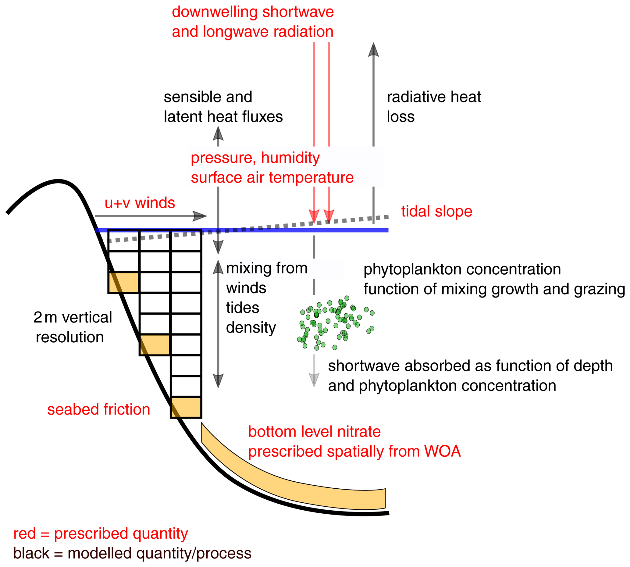
Figure 1 Schematic description of the processes accounted for in S2P3-R v2.0 and prescribed quantities, both forcings and constants. WOA stands for World Ocean Atlas.

4 Practical advances from S2P3

The practical developments made to version 2.0 of S2P3-R fall into two categories: (1) how the model runs and (2) how to generate the data used to set up and force the model.

The initial spatial implementation of S2P3 (S2P3-R v1.0) focused on what could be achieved by running S2P3 in a regional sense and as such provided Bash scripts which ran individual instances of the 1-D model for each of the latitude–longitude locations specified in a domain file containing depth and tidal forcing data. S2P3-R v2.0 makes several changes to reduce the amount of input–output associated with this approach and distributes the processing of water columns over multiple processor cores. This is done by (1) re-writing the code which runs the underlying Fortran model code from Bash to Python using the multiprocessing module, (2) reading the depth and tidal data from file once, then passing it from memory to the Fortran code for each point, and (3) accumulating the output annually and writing this year by year to NetCDF or text files. The model has been modified to run one year at a time, writing output then “resubmitting” to allow long, high-resolution or large-spatial-domain simulations to be performed without hitting memory or submission length limits.

The independence of each grid point, combined with the developments to consolidate reading or writing data to disc, means that the model scales very efficiently when more or fewer processor cores are used (Fig. 2).

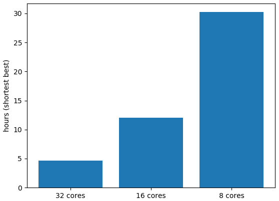
Figure 2 Processing time in hours to complete one year of simulation at 0.2^∘ resolution in a “global” (65^∘ S–65^∘ N, 180^∘ W–180^∘ E) configuration spanning water depths of 10–100 m. The high latitudes were removed because the model assumes constant salinity and the model does not include a representation of sea ice. Simulations were undertaken on an AMD 2990WX 32-core 3 Ghz processor with multi-threading.

Model developments around usability include (1) translating the Fortran code so it can be compiled with the open-source GFortran compiler rather than the proprietary ifort compiler and by doing so improving accessibility, (2) providing the user option to generate output files directly in NetCDF format, (3) providing an interface for prescribing which output diagnostics the user wishes to produce and (4) the provision of scripts and associated readme files to enable simple generation of all of the required input files (see Code Availability section). These files are the domain (which specifies the depth and tidal forcing for each model grid point), nutrient ancillary and meteorological forcing files (Fig. 3). The input generation scripts, the input data they require and how the outputs are used by the main model are detailed in Fig. 3. The practicalities of how to obtain and run the scripts and associated data are detailed in the Code Availability section and supplied readme files (see Code Availability section).

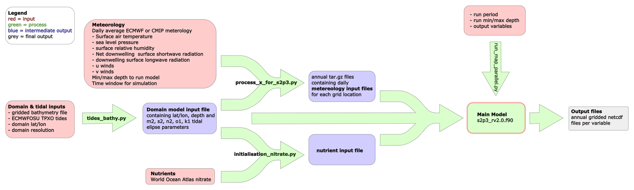
Figure 3 Overview of the S2P3-R v2.0 framework, which includes the model and runscript but also separate scripts to generate the required input files. The arrows show where externally available data or the output from one component of S2P3-R V2.0 is supplied to another component or output.

5 Global evaluation

S2P3-R v2.0 is an intentionally simple model. By ignoring lateral advection, one should expect to see model temperature biases in regions of heat convergence or divergence, i.e. where significant amounts of heat are imported or exported through advection, or local dissipation rates are enhanced through horizonal processes. The fact that a region may experience a temperature bias does not itself mean the model is not useful in that region. Despite biases in average temperatures, the model may still capture variability on the timescales of interest. The model variability may however be compromised if there is a temperature bias at low ambient temperatures, where the non-linearity of the equation of state of seawater reduces the sensitivity of density to temperature variability. This limits the applicability of S2P3-R v2.0 in cold waters, and alongside the specification of constant salinity and omission of sea ice processes, this means that the evaluation of the model has been restricted to the subpolar and lower-latitude ocean (<65^∘ N/S). The evaluation presented here is intended to allow potential model users to identify whether S2P3-R v2.0 is an appropriate tool to use for the question and location they are interested in. We first evaluate the global performance of the model, then focus evaluation on a midlatitude and then a low-latitude region. Evaluation in each section begins with the physical variables, then moves on to the biological component of the model.

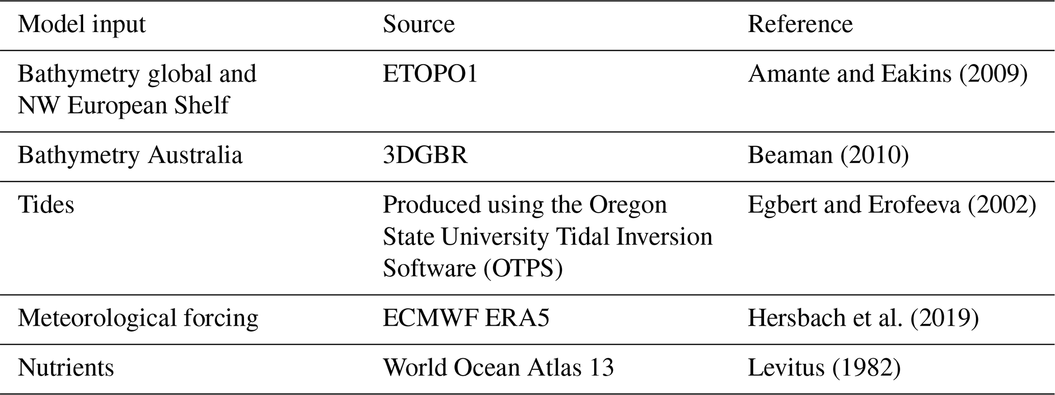
The model simulations presented here have been set up at 0.2^∘ spatial resolution using the input fields described in Table 1.

Table 1 Model inputs.

5.1 Global physical evaluation

An initial comparison of model sea surface temperature (SST) against satellite SSTs (Merchant et al., 2019) at a global scale indicates that the model displays its smallest biases in the subtropics to subpolar regions (Fig. 4). The prevalence of warm biases in the tropics and cool biases in the high latitudes is consistent with export and import or warm waters from and to these regions, respectively (Fig. 4). To allow potential users to examine model performance in their regions of interest in greater detail, the data underlying Fig. 4 are made available as described in the Data Availability section.

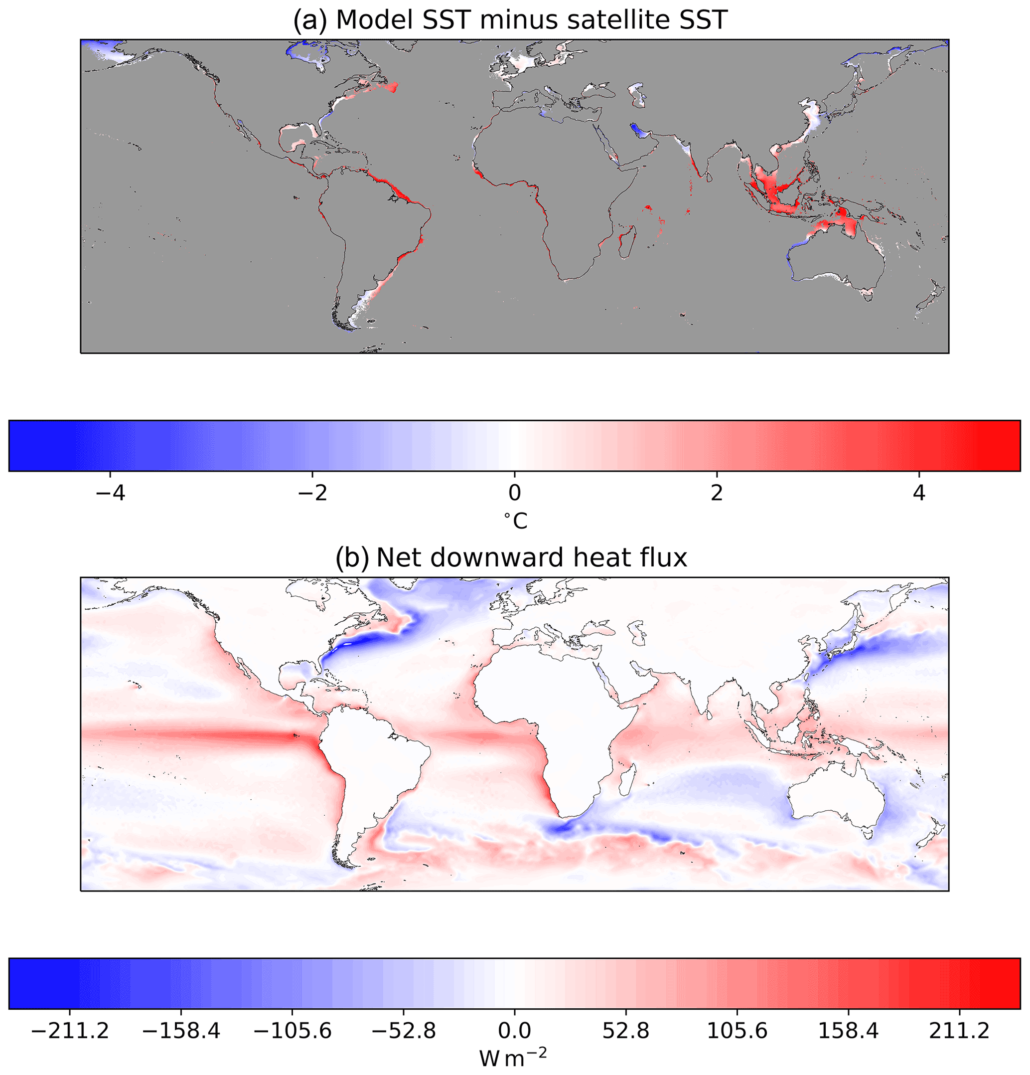
Figure 4 (a) Model SST simulation minus satellite SST data averaged between 1 January 2006 and 31 December 2016. White indicates that the model is displaying no surface temperature bias, red indicates the model displays a warm bias, and blue indicates the model displays a cool bias. The model was forced with atmospheric data from ERA5 (Hersbach et al., 2019). (b) Net surface downward heat flux calculated from the ECMWF ERA5 reanalysis (Hersbach et al., 2019). Where this is positive, there is a net heat flux into the ocean. So, assuming that system is approximately at steady state, heat is advected out of these areas. Where the net downward heat flux is negative there is advection of heat into this region. S2P3-R V2.0 does not account for lateral advection, so one would anticipate that the model will display a warm bias in regions where heat is typically advected from (i.e. tropics) and cool biases where heat is advected to (i.e. high latitudes).

Beyond calculating the surface heat budget based on atmospheric forcings, the model skill in simulating surface temperatures comes from vertical mixing processes which exchange heat between the surface and subsurface layers as a function of temperature induced density differences and wind and tide stress. In line with this, we find that large SST biases are more prevalent at low M2 tidal amplitudes (Fig. 5). While this analysis indicates that strong tidal mixing can contribute to a skilful simulation, it does not appear that tidal magnitude provides a rule to determine where best to use this model. Stratification is highly seasonal in the midlatitudes (30 to 60^∘ north or south), with summer stratification typically corresponding to areas of weak tidal mixing, and a pervasive loss of stratification during the winter. If strong tides played a first-order role in model skill, one would expect to see smaller model biases in the summer than winter across the midlatitudes (Fig. 6); instead, we see little seasonality in the bias in much of the midlatitudes (e.g. Northwest European Shelf and Patagonian Shelf), stronger summer than winter bias in the South China Sea and Bering Sea, and only smaller summer than winter biases in the Scotian and southern Brazilian shelves.

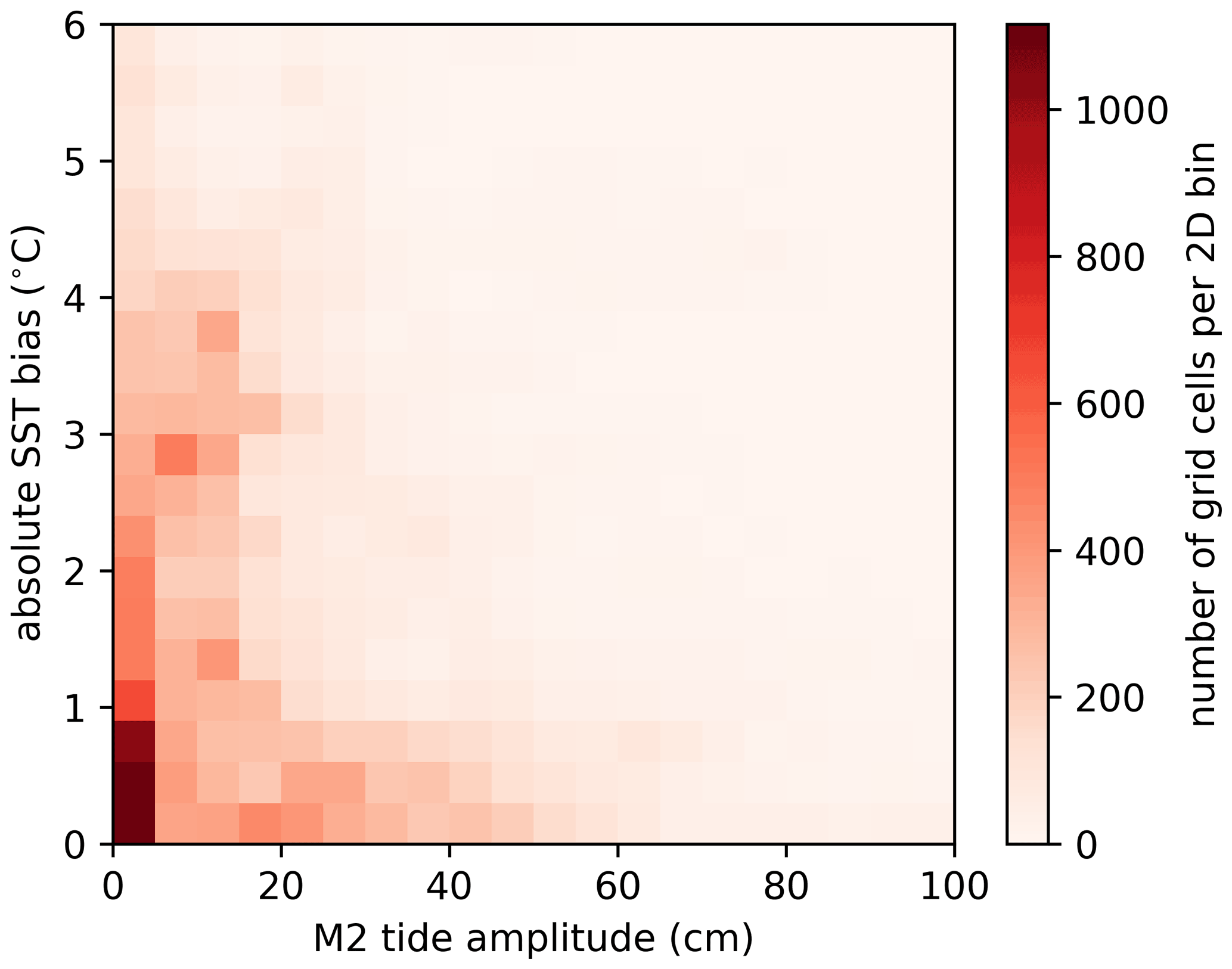
Figure 5 2-D histogram demonstrating the relationship between tidal amplitude (M2 tide) and absolute annual mean SST difference between the model and satellite data.

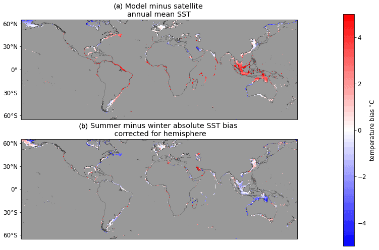
Figure 6 Annual mean SST bias (a) and difference in absolute SST bias between summer and winter (b). In panel (b), blue indicates that the summer months (June, July, August in the Northern Hemisphere; December, January, February in the Southern Hemisphere) display a smaller absolute bias than the winter months (December, January, February in the Northern Hemisphere; June, July, August in the Southern Hemisphere).

Despite the model displaying average temperature biases across some regions of up to ∼3 K, there is no consistent relationship between such biases and the model's ability to correctly simulate year-to-year variability (Fig. 7). More than half of the year-to-year variability is captured by ∼60 % of the simulated grid cells (Fig. 8). Squared Pearson's product moment correlations (R²) calculated between (i) annual mean SST time series at each grid point from the ERA5 forced S2P3R v2.0 simulations and (ii) satellite SST data (Merchant et al., 2019) from 2006–2016 (inclusive) demonstrate high levels of skill in areas such as north of Australia, the Java Sea and the Bering Sea (Fig. 7), despite these areas displaying significant positive or negative temperature biases (Fig. 4). Conversely, the northern South China Sea and southern Australia display low skill at capturing interannual variability (Fig. 7), despite the model displaying low temperature biases in these regions (Fig. 4). In the case of the South China Sea, this may relate to highly variable riverine freshwater influences on stratification.

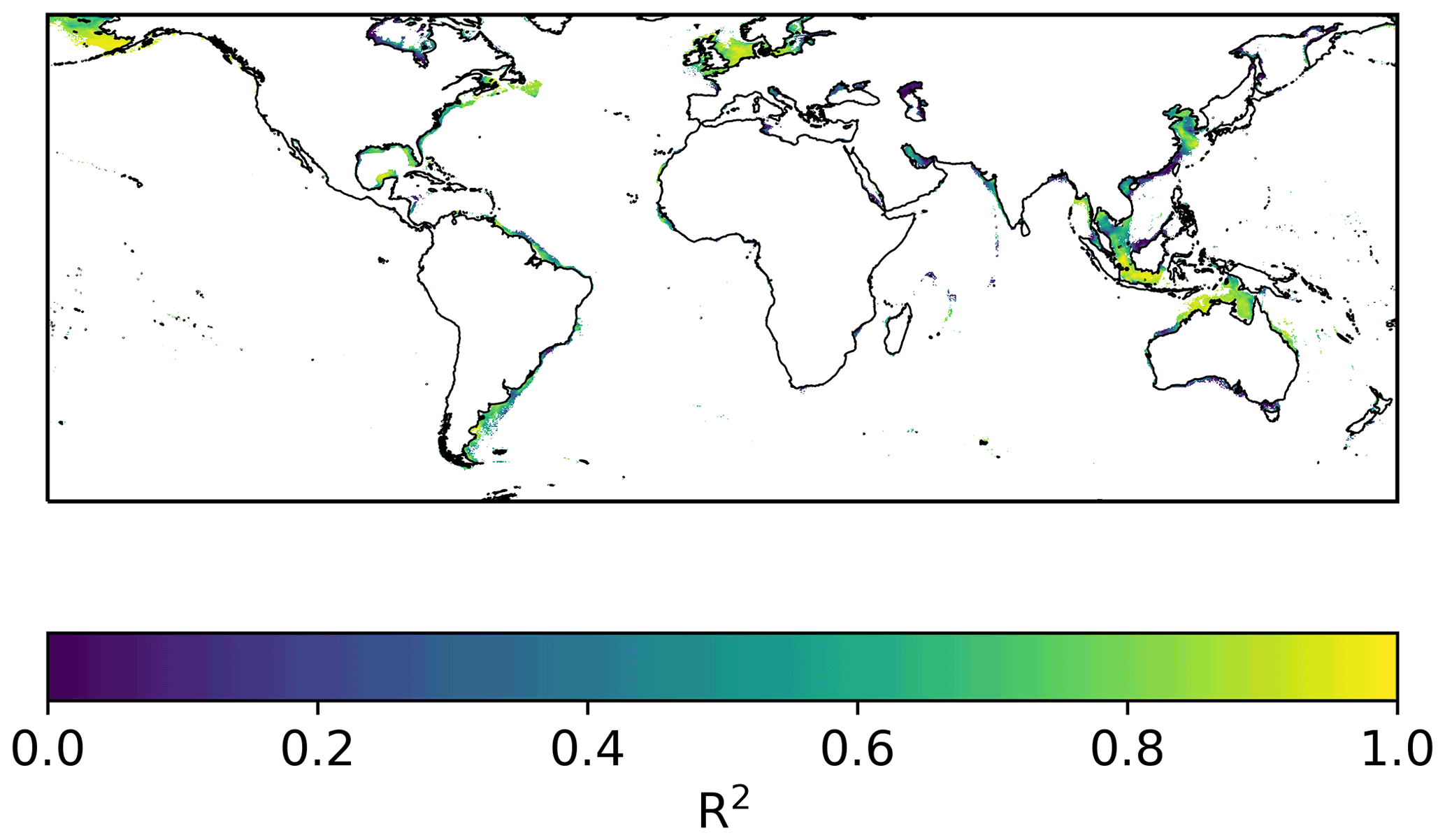
Figure 7 Pearson's R² calculated between annual mean model SST simulation and annual mean satellite SST data (Merchant et al., 2019) between 2006 and 2016.

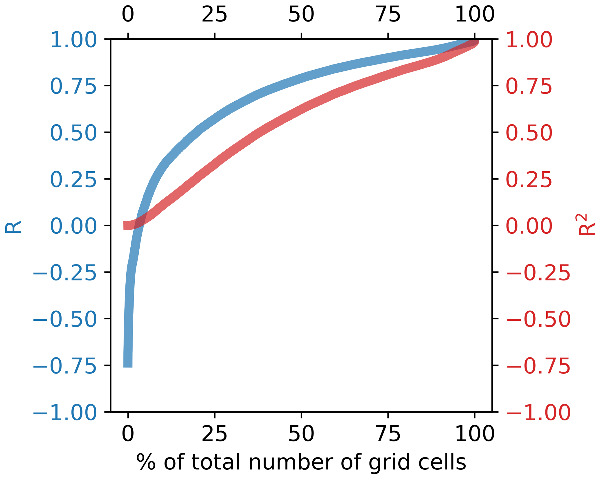
Figure 8 Sorted R and R² values from all grid cells calculated from global shelf-sea SST simulation correlation with satellite SST (Fig. 7).

5.2 Global biogeochemical evaluation

The biological component of S2P3 remains unchanged from previous versions, apart from the addition of a spatially varying nutrient field derived from the World Ocean Atlas (Levitus, 1982) to which the bottom water nitrate is relaxed. S2P3 has previously been used to investigate biological questions including investigating the drivers of timing of spring blooms in response to stratification (Sharples et al., 2006) and to explore the impact of tidal cycles on productivity (Sharples, 2008) for typical Northwest European Shelf seas. More recently, a version of S2P3 has been developed to better represent the impacts of grazing and to include the impact of photo-acclimation on phytoplankton growth (Bahamondes Dominguez et al., 2020).

Evaluation of the model's biological performance at a global scale is more challenging than the evaluation of surface temperature, because satellite chlorophyll-a products are often unreliable in shallow waters, where suspended sediment, coloured dissolved organic matter (CDOM) and bottom reflection influence the retrievals considerably (Darecki and Stramski, 2004). The analysis presented here uses the European Space Agency Climate Change Initiative (ESA CCI) chlorophyll-a product data (Sathyendranath et al., 2020) but filters out waters shallower than 70 m (Sathyendranath et al., 2019) to avoid the issues mentioned above. The model demonstrates low (<0.2 mg m⁻³) chlorophyll-a biases when compared to satellite estimates in all regions apart from southeast Asia, Australia, the Baltic Sea and the northern Bering Sea (Fig. 9), with the most extensive areas of bias being southeast Asia and Australia. These are also areas of high SST bias (Fig. 4), although there is no straightforward relationship between regions of SST and regions of chlorophyll-a bias. Phytoplankton growth in the model is a function of, amongst other factors, temperature and PAR. Overestimation of chlorophyll-a may therefore be a response to positive seawater temperature biases, or both may be responding to a positive shortwave radiation bias.

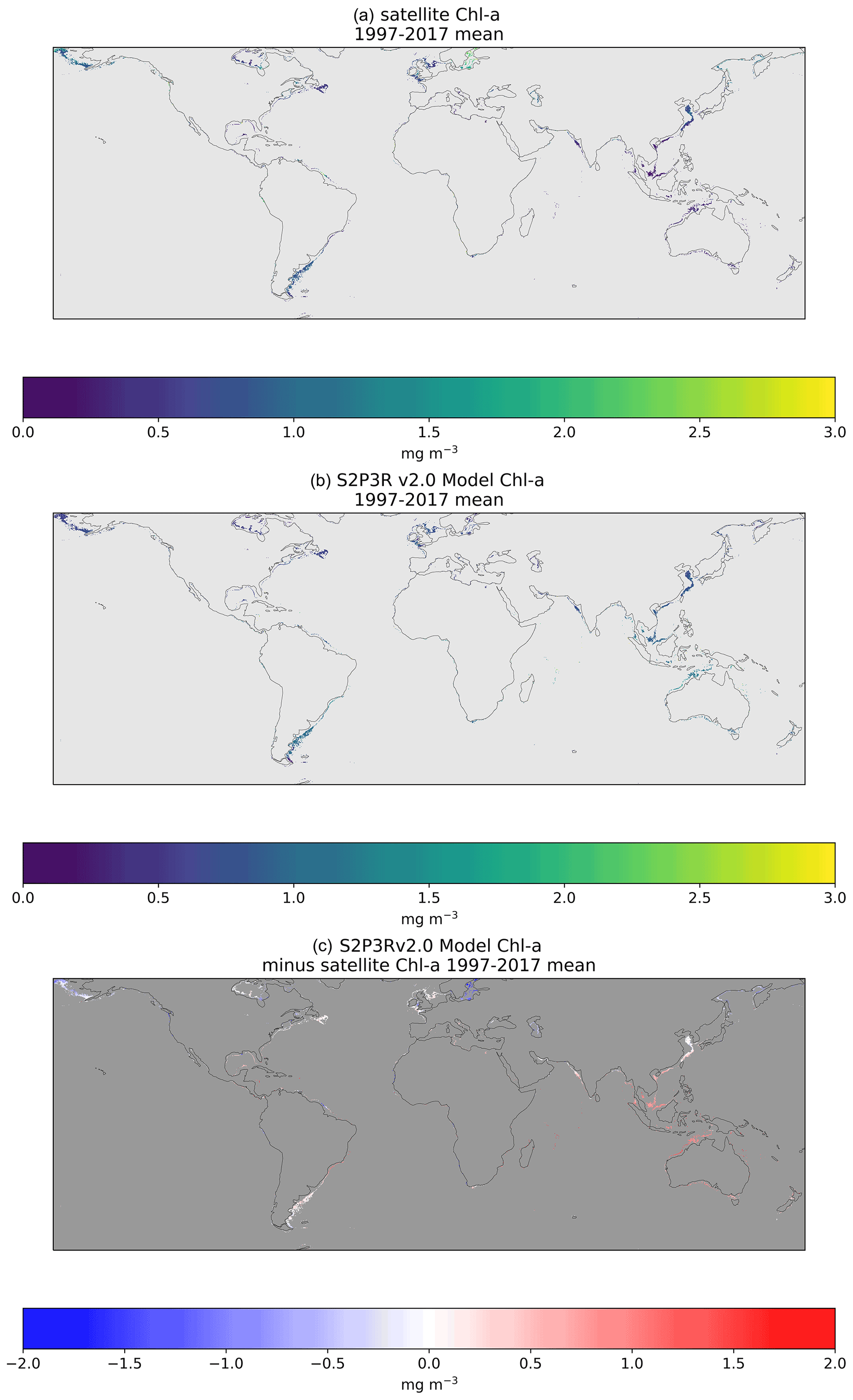
Figure 9 Comparison of surface level chlorophyll-a concentrations with satellite based chlorophyll-a estimates (Sathyendranath et al., 2020). Figures present an annual mean of all data available between 1997 and 2017 inclusive. Satellite data are filtered to include minimised issues associated with case-2 waters by selecting water ≥70 m water depth. The nutrient data to which the water in the model's bottom level was relaxed to are taken from the winter values in World Ocean Atlas for each hemisphere.

To facilitate a more detailed understanding of the model performance, we now evaluate the model in one midlatitude region, the Northwest European Shelf, then one lower-latitude region, the Great Barrier Reef.

6 Northwest European Shelf physical evaluation

The Northwest European Shelf is both typical of the midlatitude regions, where the assumptions made in this modelling framework appear to work well (Fig. 4), and it is a large area of shallow water which has previously been studied in detail both observationally (e.g. Smyth et al., 2015) and using state-of-the-art 3-D models (e.g. Graham et al., 2018).

Forced with the ERA5 atmospheric data (Hersbach et al., 2019), S2P3-R v2.0 simulates the time-averaged SST within 0.5 K across much of the Northwest European Shelf (Fig. 10). The model also simulates the trend and interannual variability in SST well in the North Sea, English Channel and Irish Sea (Fig. 11), despite the North Sea and English Channel displaying cool and warm temperature biases of approximately 0.5 K respectively (Fig. 11). The cool bias in the northern North Sea is consistent with the model not accounting for the inflow of relatively warm Atlantic Water via the Dooley Current between Orkney and Shetland (Dooley, 1974; Marsh et al., 2017; Sheehan et al., 2020).

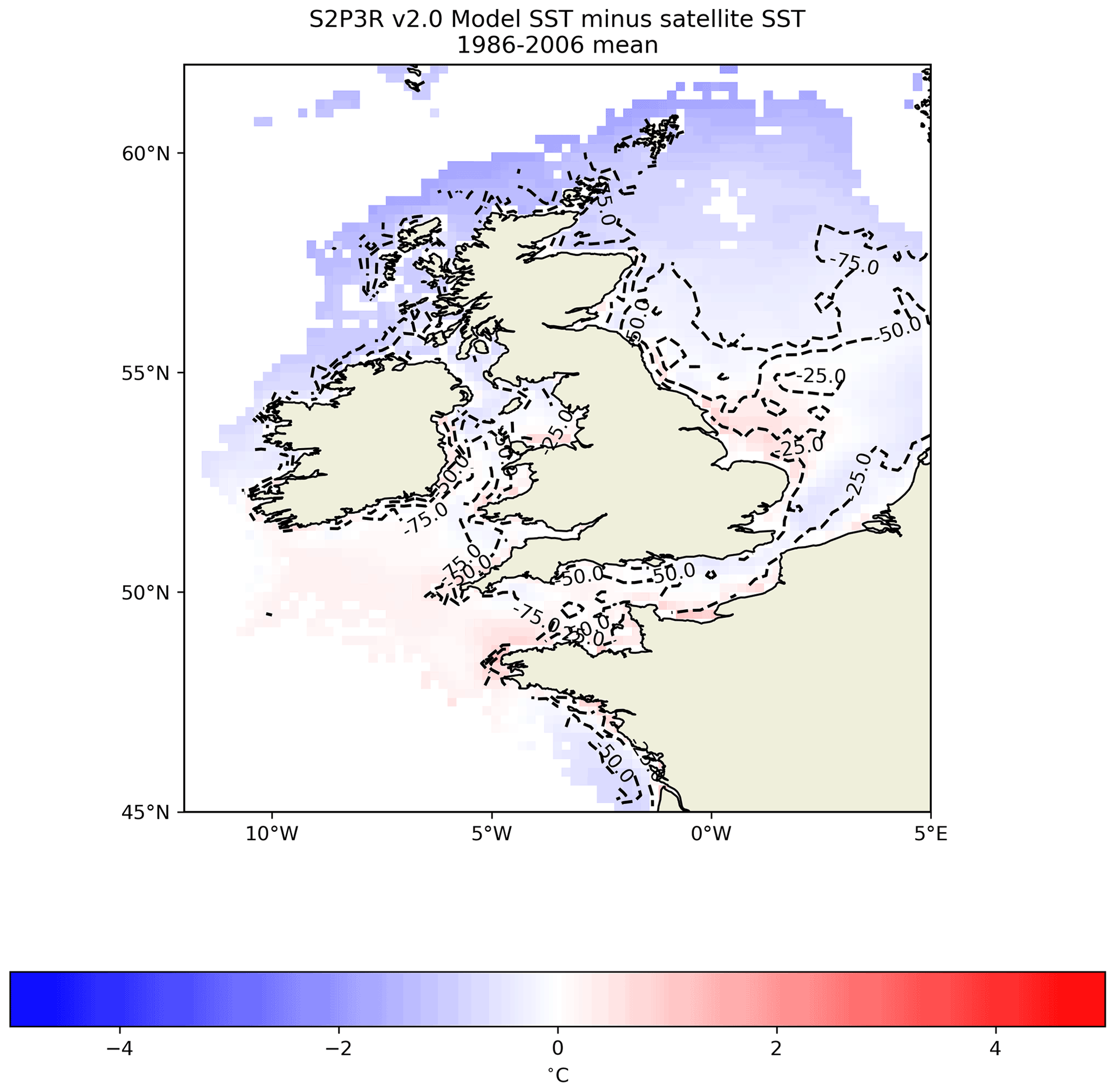
Figure 10 S2P3R v2.0 SST averaged between the years 1986 and 2006 inclusive minus satellite SSTs (Merchant et al., 2019) averaged over the same interval. Labelled dashed lines illustrate bathymetry in metres.

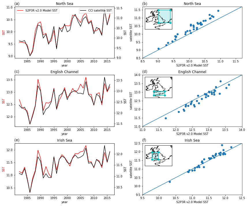
Figure 11 S2P3R v2.0 SST averaged annually and across the three regions highlighted in inset maps and annually averaged satellite SSTs (Merchant et al., 2019) from the same regions.

Bottom water temperatures can be examined at individual locations using mooring data, as done in Marsh et al. (2015), or at sparse locations against gridded data (e.g. Good et al., 2013), but to facilitate a more spatially complete assessment we here turn to state-of-the-art model output, generated by the 1.5 km Nucleus for European Modelling of the Ocean (NEMO) shelf Atlantic Margin Model (AMM15) (Graham et al., 2018). We find that S2P3-R v2.0 replicates the average values and interannual variability in bottom water temperatures in the North Sea, English Channel and Irish Sea captured by the AMM15 model (Graham et al., 2018) with biases of less than 0.5 K and R² values of 0.92, 0.84 and 0.93 the North Sea, English Channel and Irish Sea, respectively (Fig. 12). While the AMM15 model is not a perfect surrogate for observations, this comparison gives us confidence in these regions that the use of the highly computationally efficient S2P3-R v2.0 model to a first order gives us comparable bottom water temperature results to a state-of-the-art and computationally demanding three-dimensional modelling system.

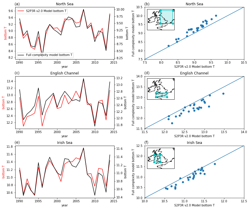
Figure 12 S2P3R v2.0 bottom water temperatures averaged annually and across the three regions highlighted in inset maps and annually bottom water temperatures from these same regions taken from a state-of-the art shelf sea model hindcast (Graham et al., 2018).

Northwest European Shelf biogeochemical evaluation

S2P3R v2.0 underestimates surface chlorophyll-a when compared to annual mean satellite derived estimates (Sathyendranath et al., 2020) across most of the Northwest European Shelf by 0.25 to 0.50 mg m⁻³ (Fig. 13). The smallest bias is seen in the North Sea and the largest in the Irish Sea (Fig. 13).

Figure 13 Comparison of Northwest European Shelf surface level chlorophyll-a concentrations with satellite based chlorophyll-a estimates (Sathyendranath et al., 2020). Figures present an annual mean of all data available between 1997 and 2017 inclusive. Dashed lines represent 20 m depth contours. Satellite data are filtered to minimise the influence of case-2 waters by focusing on water ≥70 m water depth.

The seasonal and interannual variability of phytoplankton production, and therefore chlorophyll-a concentration are strongly influenced by changes in stratification. Where the water column is mixed throughout the year (e.g. English channel and southern North Sea), phytoplankton growth tends to display a single peak governed to a first order by the cycle of solar irradiance and the availability of nutrients, with development of the peak slowed by mixing of phytoplankton into deeper, poorly lit, waters (e.g. Fig. 14a, c, e, g, i, j) (Wafar et al., 1983). Where the water column is seasonally stratified and winter mixing has removed any upper-water column nutrient limitation potential, a spring bloom typically develops as the mixed layer – defined by turbulence levels (Chiswell, 2011; Chiswell et al., 2015) – shallows across a seasonally deepening critical depth, shallower than which light-limited phytoplankton production exceeds approximately depth-invariant phytoplankton losses (Sverdrup, 1953). In these seasonally stratified waters, an autumn bloom (and therefore second chlorophyll-a peak) may also develop as cooling results in buoyancy loss from the surface or winds increase turbulence, and the mixed layer deepens and refreshes what have become nutrient-limited sunlit waters, with nutrients from deeper in the water column (Findlay et al., 2006). This potentially skewed, bimodal distribution is captured by the model in seasonally stratified sites (Fig. 14c, k, o). While in the central North Sea and Celtic Sea, the seasonal evolution of model chlorophyll-a concentrations match closely with that inferred from observations (Fig. 14c, k, o), at most sites the model fails to capture the full complexity of the seasonal signal. The model also fails to capture the interannual variability in chlorophyll-a at those sites where long-enough observational time series exist to assess this (Fig. 14). The lack of evidence for correctly simulated interannual variability potentially reflects the importance of processes not represented in this model such as photo-acclimation (Bahamondes Dominguez et al., 2020), grazing (Bahamondes Dominguez et al., 2020) and phytoplankton species composition (Barnes et al., 2015) in controlling interannual variability or the importance of variability in nutrient flux across the shelf break (Holt et al., 2012) and from rivers (Capuzzo et al., 2018).

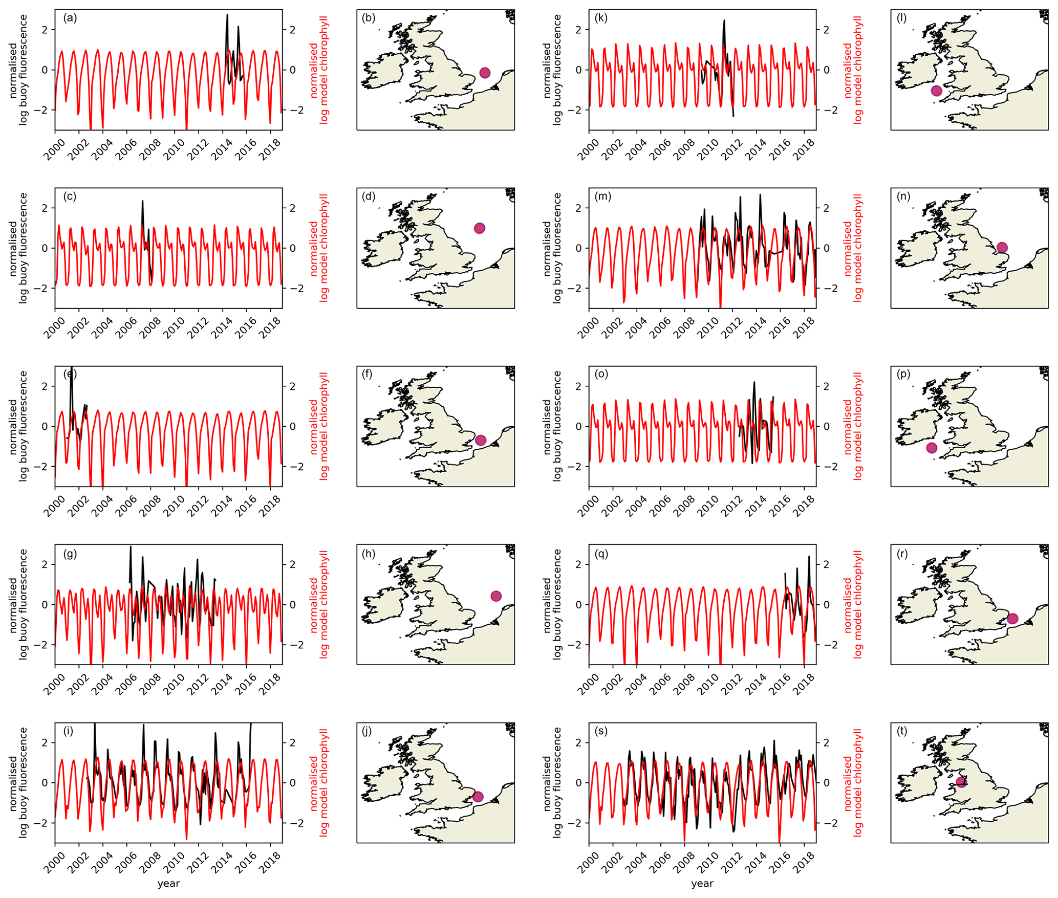
Figure 14 Comparison of model chlorophyll-a time series (red) with chlorophyll-a fluorescence measurements (black) made on 10 autonomous buoys situated round the UK as part of the Cefas SmartBuoy network (Sivyer, 2016). Both datasets have been averaged monthly and logged, had the time series mean removed and have been normalised by their standard deviation. Fluorescence data have been filtered to include only that collected between 18:00 and 06:00 LT to avoid quenching of the signal by sunlight. Maps on the right-hand side illustrate the location of each buoy. Note that buoys have been operational over different time windows.

7 Great Barrier Reef physical evaluation

Moving to the low latitudes where SST biases in the S2P3R v2.0 model are typically larger than they are in the midlatitudes (Fig. 4), a simulation has been undertaken which encompasses the Great Barrier Reef (GBR). The GBR is well instrumented, allowing analysis of subsurface as well as surface temperatures in this region.

The modelled SSTs in the GBR display a positive bias relative to satellite SSTs in the north and negative bias in the south (Fig. 15). This may relate to the fact that the model does not simulate lateral advection, which will be exporting heat from the north to the south in the East Australian Current.

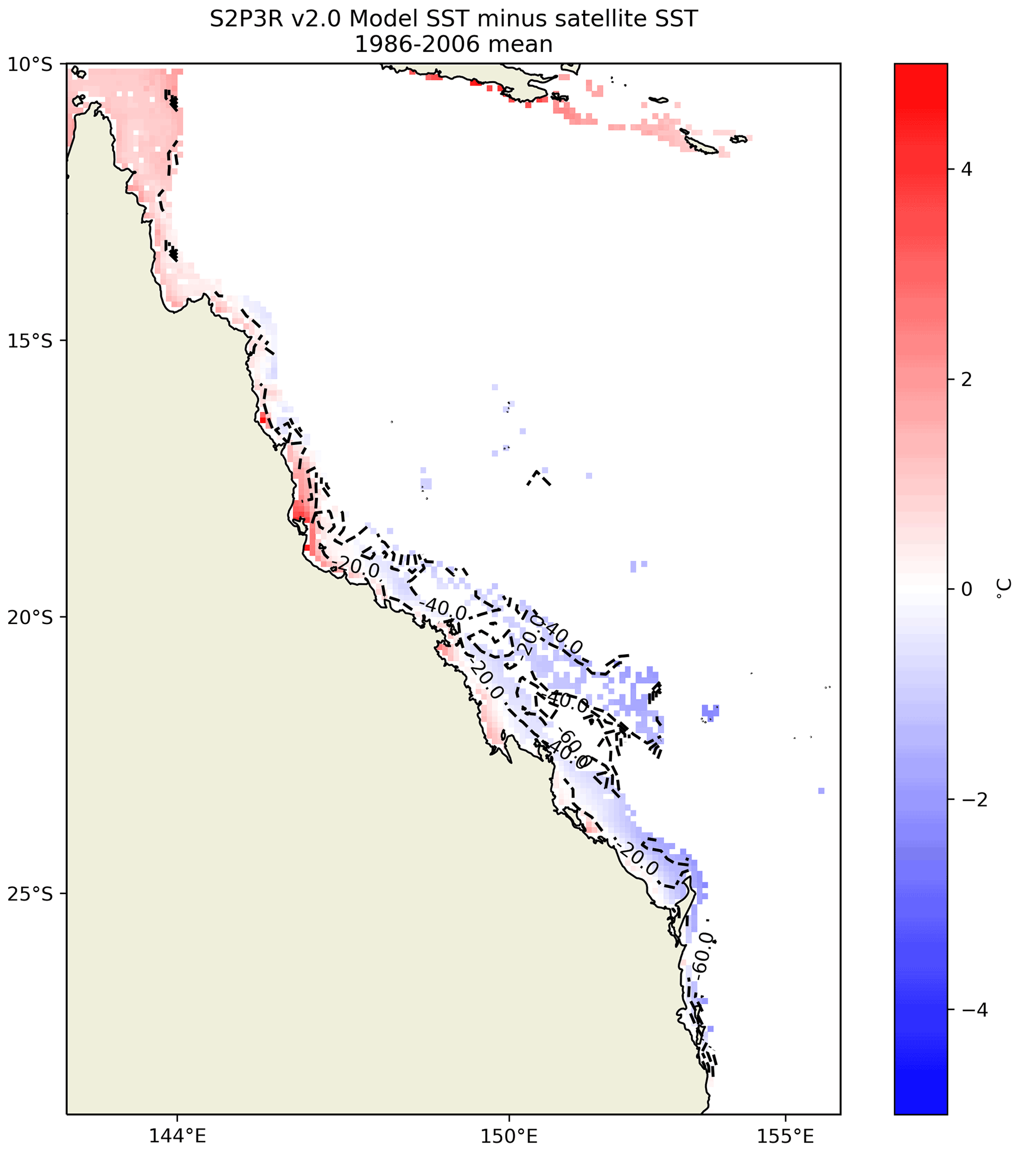
Figure 15 S2P3R v2.0 SST averaged between 1986 and 2006 inclusive minus satellite SSTs (Merchant et al., 2019) over the same interval. Labelled dashed lines show bathymetry in metres.

S2P3R v2.0 appears to capture much of the interannual variability observed in SSTs over the GBR since the early 1980s (Fig. 16) but with a temperature bias of <0.5 K (Fig. 15). The simulation however appears to erroneously simulate a stepwise cooling around the year 2000, which compromises the overall correlation between model and satellite SSTs (Fig. 16). This stepwise cooling may reflect changes in the assimilation of observations into the ERA5 reanalysis product which is used to force the model.

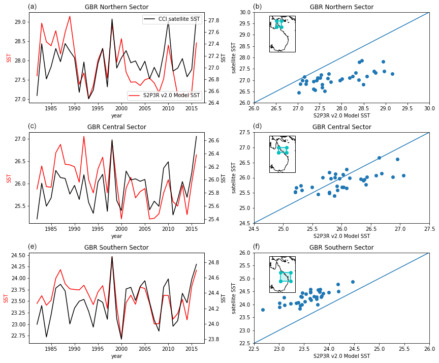
Figure 16 Comparison of interannual SST variability between S2P3R v2.0 and satellite (Merchant et al., 2019) over the GBR, subdivided into three latitudinally delineated regions. These regions are identified in the inset maps.

While a state-of-the-art regional model for the GBR region exists (Steven et al., 2019), a long validated hindcast is not available to allow evaluation of the S2P3R V2.0 simulation of bottom water temperatures in the GBR analogous to that presented here for the Northwest European Shelf. The GBR is however instrumented with an extensive mooring network, making up part of the IMOS FAIMMS (Integrated Marine Observing System, Facility for Automated Intelligent Monitoring of Marine Systems) sensor network. The following IMOS FAIMMS sites have been use: Heron Island South Shelf (GBRHIS, Integrated Marine Observing System, 2009a); Lizard Island Shelf (GBRLSH, Integrated Marine Observing System, 2009b); Palm Passage Shelf (GBRPPS, Integrated Marine Observing System, 2009d), Yongala mooring (NRSYON, Australian Institute of Marine Science, 2020); One Tree Island Shelf mooring (GBROTE, Integrated Marine Observing System, 2009c) and the Ningaloo mooring (NRSNIN, Integrated Marine Observing System, 2017). The locations of the moorings utilised in the evaluation presented here are highlighted in Fig. 17.

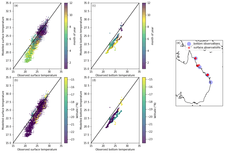
Figure 17 Comparison of S2P3R v2.0 surface (a, b) and bottom (c, d) temperatures against mooring observations from IMOS and FAIMMS and moorings (Integrated Marine Observing System; IMOS). Facility for the Automated Intelligent Monitoring of Marine Systems – FAIMMS; GBRHIS: Heron Island South Shelf mooring component of the GBR mooring array; GBRLSH: Lizard Island Shelf mooring component of the GBR mooring array; GBRPPS: Palm Passage Shelf mooring component of the GBR mooring array; Northern Australia Automated Marine Weather and Oceanographic Stations, sites: Yongala mooring (NRSYON); GBROTE: One Tree Island Shelf mooring component of the GBR mooring array; IMOS – ANMN National Reference Station (NRS) Ningaloo mooring (NRSNIN). The x−y values of the data presented in plots on the top and bottom (a and b, and c and d) are identical but are coloured to highlight where temporal and geographical biases exist in the model output. Seabed observations are considered here to be those falling within 5 m of the site depth for each mooring. The map shows the location of surface (red) and bottom (blue) temperature mooring observations used in model evaluation over the GBR.

In situ observations indicate that a cool bias exists in the modelled SSTs, but this is restricted to austral winter months (Fig. 17c). The fact that a warm bias is not evident in the mooring data, as it is in the satellite SST data (Fig. 15), may result from a sampling bias within the mooring dataset towards deeper waters. Modelled bottom water temperatures from the lower-latitude mooring sites present a cool bias, but a linear relationship when compared with observational data (Fig. 17d). The cool bias may reflect the fact that the model output against which the observations are compared represent a mean value across a ∼10 km² grid cell and, for example, may well therefore not be simulating the conditions at the same depth as the observations are made.

Great Barrier Reef biogeochemical evaluation

A comparison is made between the S2P3R v2.0 simulation of chlorophyll and annually averaged ESA CCI long-term satellite chlorophyll data (Sathyendranath et al., 2020). The ESA CCI long-term satellite chlorophyll product is focused on case-1 waters (Sathyendranath et al., 2019). The comparison presented here is therefore restricted to water depths ≥70 m, a compromise which allows us to exclude the most coastally influenced waters while maintaining moderate spatial coverage. The S2P3R v2.0 simulation of chlorophyll displays low negative biases <0.2 mg m⁻³ (Fig. 18). These biases are considerably lower than those simulated on the Northwest European Shelf (Fig. 13), the region within which the model was originally designed to investigate chlorophyll seasonality (Sharples et al., 2006).

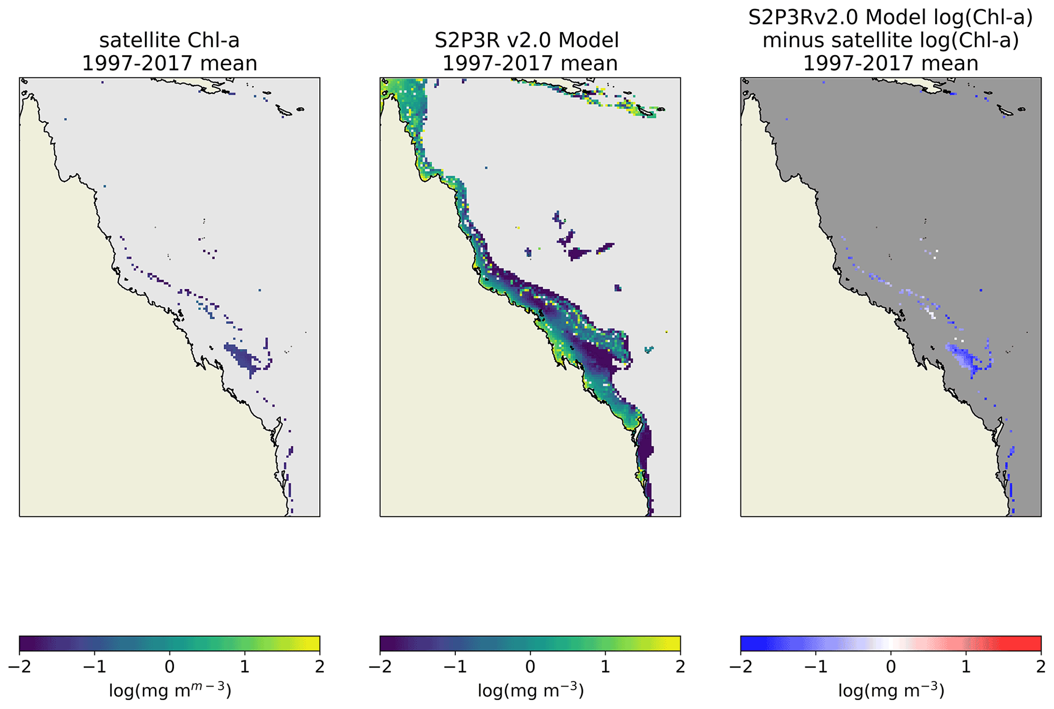
Figure 18 Comparison of GBR surface level chlorophyll-a concentrations with satellite based chlorophyll-a estimates (Sathyendranath et al., 2020). Figures present an annual mean of all data available between 1997 and 2017 inclusive. Satellite data are filtered to include just water ≥70 m to minimise contamination by case-2 waters.

An evaluation of the model's ability to simulate the seasonal cycle and interannual variability in chlorophyll-a in the GBR region has been conducted using moored buoy fluorescence data, as done for the Northwest European Shelf, but with more restricted temporal coverage (Fig. 19). Unlike the spring/autumn bloom-dominated seasonal evolution of chlorophyll-a experienced in many temperate sites, the seasonal cycle simulated by the model and illustrated by the observations across the GBR sites examined here follows a relatively smooth oscillation with the peak values in the model data occurring in late summer (Fig. 19). In contrast to many of the Northwest European Shelf sites, this behaviour likely results from the intersection of the critical depth (Sverdrup, 1953) with the seabed at these high-light and shallow locations. The incomplete or short lengths of the GBR fluorescence observational datasets mean that it is not possible to undertake a detailed investigation of interannual variability; however, the longest of the mooring datasets (Fig. 19k) exhibits its lowest chlorophyll-a peaks in the same years as those simulated by the model (2018 and 2019). In a typically oligotrophic setting, like much of the GBR, one might expect year-to-year variability to be dominated by injections of nutrients from the shelf break or the coast (Furnas and Mitchell, 1986). Despite the model not representing these processes, it nevertheless simulates considerable interannual variability, indicating the potential for atmospheric and vertical ocean dynamics drivers of such variability.

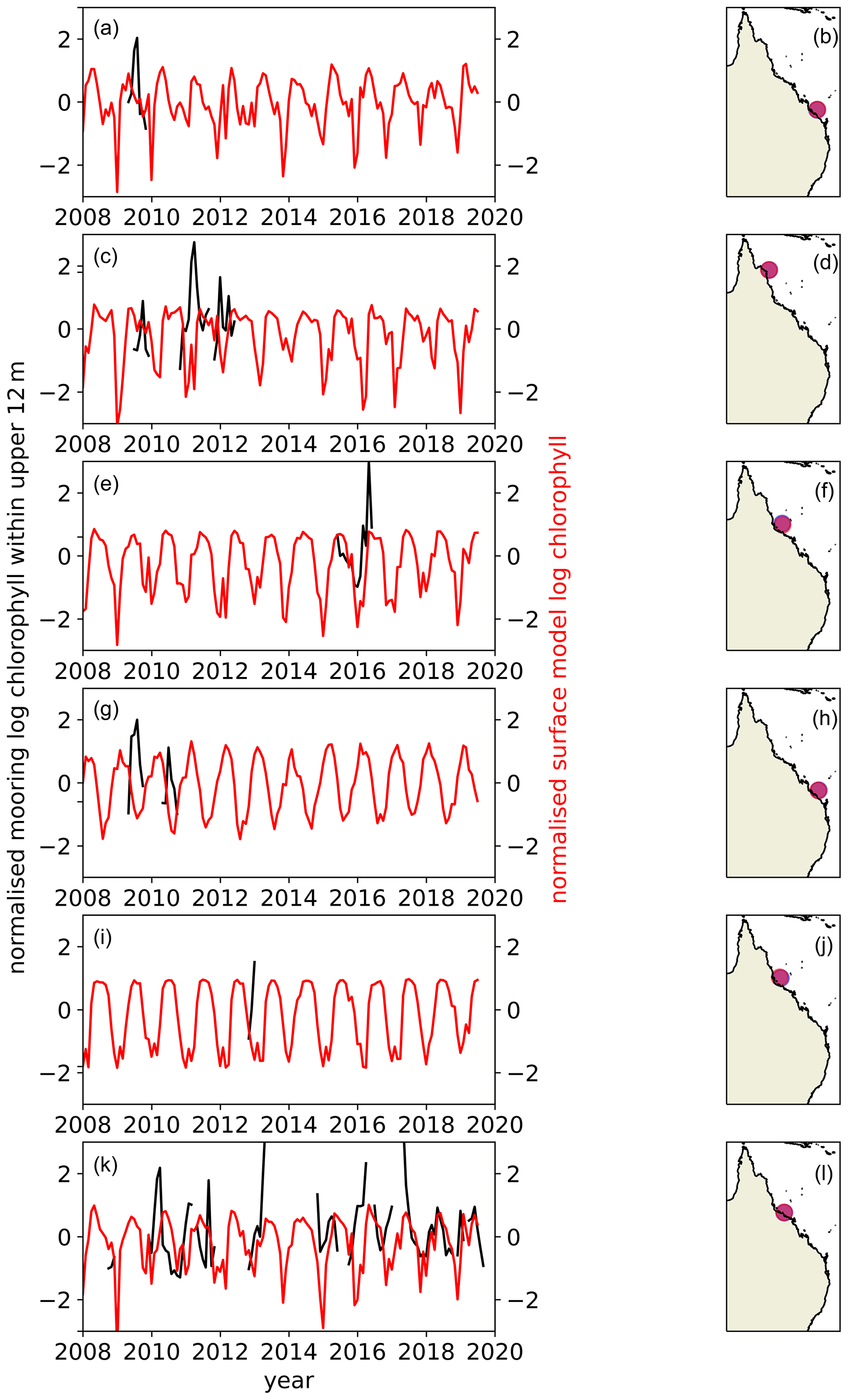
Figure 19 Comparison of model chlorophyll-a time series (red) with chlorophyll-a fluorescence measurements (black) made on six moored buoys situated down the GBR as part of the IMOS FAIMMS. Both datasets have been averaged monthly and logged, had the time series mean removed and have been normalised by their standard deviation. Surface level data were not available for all sites, so data represent an average over the top 12 m of the water column to improve spatial data coverage.

8 Summary and discussion

Forced by observation-derived atmospheric conditions, a simulation spanning the shelf seas of the global tropical-to-subpolar ocean at approximately 10 km² resolution captures >50 % of the observed interannual SST variability between 2006 and 2016 in ∼60 % of the grid cells, and greater than 80 % of the interannual SST variability in ∼20 % of the grid cells (Fig. 8). This tells us that a large part of the SST variability in a significant component of our global shelf seas is atmospherically forced rather than forced by variable lateral exchanges with the deep ocean or runoff. When compared to satellite data (Merchant et al., 2019), 61 % of grid cells however present an SST bias of greater than 1 K and 42 % present an SST bias of greater than 2 K, highlighting limitations to the simple modelling approach.

Together, analysis of SST variability and SST bias indicates that there are significant areas of our global shelf seas where the model should be used with extreme caution. These regions are likely to be those which have (1) substantial exchange of heat with the open ocean through lateral advection, (2) low tidally driven mixing and therefore a low ratio of vertical/horizontal control over SSTs (Fig. 5), (3) significant influences from local processes/properties such as riverine inputs or locally unusual bottom drag coefficients, (4) high salinity variability and low temperatures, or (5) on-shelf propagation and dissipation of the internal tide. The model could however be tuned to account for some of these influences if studies were to be undertaken with a focus on such regions.

Regional evaluation has been conducted across the Northwest European Shelf around the UK and the Great Barrier Reef. The model captures most of the observed SST trend and variability in the waters around the UK (Fig. 11), with a temperature biases of <0.5 K across most of the region (Fig. 10). S2P3R v2.0 also captures between 84 and 93 % of the variability in bottom water temperatures simulated by a state-of-the-art shelf sea model hindcast (Graham et al., 2018) for the three focal regions of the North Sea, English Channel and Irish Sea. Comparison of modelled and satellite SSTs across the Great Barrier Reef indicates that over ∼10-year intervals the model performs well, but there appear to be step changes in the modelled SST which are not seen in the satellite data. The discontinuity occurring around the year 2000 may reflect a step change in the data assimilation configuration used within the ERA5 product or data being assimilated by that product (Hersbach et al., 2018) used to provide the atmospheric forcing to S2P3R v2.0. Alternatively, the step changes may result from changes in the lateral supply of heat from the open ocean.

A particular strength of this modelling approach is likely to be in examining or predicting anomalies or extremes which occur under a consistent set of oceanographic conditions. For example, the marine heat waves associated with tropical coral bleaching tend to occur following doldrum-like condition, when there is limited advection and mixing (Skirving et al., 2011).

Observational limitations mean the model's simulation of biological production in space and time is harder to assess than that of temperature. The model however captures the broad-scale patterns of surface chlorophyll (Figs. 9, 13, 18), with a weak indication of latitudinally varying bias towards overprediction in low latitudes and underprediction in high latitudes (Fig. 9). While the model displays considerable skill in many locations at simulating intra-annual chlorophyll variability (Figs. 14, 19), it demonstrates no skill at simulating interannual chlorophyll variability. This implies that the large-scale processes which govern the seasonal progression of primary production do not also govern interannual variability. Factors such as riverine input of nutrients may dominate interannual variability in many locations (Lenhart et al., 1997). These results emphasise the importance of decadal and longer observational biogeochemical time series for assessing the skill of models at simulating those processes which are likely to govern the biogeochemical response of our shelf seas to anthropogenic climate change.

In summary, S2P3R v2.0 is a simple-to-use, computationally efficient shelf sea modelling tool ideally suited to (a) semi-dynamically downscale climate projections, (b) undertake large-scale, long or large-ensemble projections, (c) use after careful evaluation by management or policy groups without access to large technical or computational resources. The objective assessment of the model presented here will hopefully guide potential users as to whether S2P3R v2.0 is the tool to answer their questions. Where S2P3R v2.0 is considered to be an appropriate tool, we would encourage local assessment of the data presented here at a global scale and hope to facilitate this through the provision of these data (see Data Availability section). Finally, within the Code Availability section of this paper, we provide the model code, code required to produce the model forcing datasets, and an example model setup with pre-prepared forcing data, and within the readme file, we provide step-by-step instructions for setting up and running the model.