the Creative Commons Attribution 4.0 License.
the Creative Commons Attribution 4.0 License.
 | 11 Oct 2021
The Lagrangian-based Floating Macroalgal Growth and Drift Model (FMGDM v1.0): application to the Yellow Sea green tide
Fucang Zhou
Dongyan Liu
Pingxing Ding
Changsheng Chen
Xiaodao Wei
Massive floating macroalgal blooms in the ocean result in many ecological consequences. Tracking their drifting pattern and predicting their biomass are essential for effective marine management. In this study, a physical–ecological model, the Floating Macroalgal Growth and Drift Model (FMGDM), was developed. Based on the tracking, replication, and extinction of Lagrangian particles, FMGDM is capable of determining the dynamic growth and drift pattern of floating macroalgae, with the position, velocity, quantity, and represented biomass of particles being updated synchronously between the tracking and the ecological modules. The particle tracking is driven by ocean flows and sea surface wind, and the ecological process is controlled by the temperature, irradiation, and nutrients. The flow and turbulence fields were provided by the unstructured grid Finite-Volume Community Ocean Model (FVCOM), and biological parameters were specified based on a culture experiment of Ulva prolifera, a phytoplankton species causing the largest worldwide bloom of green tide in the Yellow Sea, China. The FMGDM was applied to simulate the green tide around the Yellow Sea in 2014 and 2015. The model results, e.g., the distribution, and biomass of the green tide, were validated using the remote-sensing observation data. Given the prescribed spatial initialization from remote-sensing observations, the model was robust enough to reproduce the spatial and temporal developments of the green tide bloom and its extinction from early spring to late summer, with an accurate prediction for 7–8 d. With the support of the hydrodynamic model and biological macroalgae data, FMGDM can serve as a model tool to forecast floating macroalgal blooms in other regions.
- Article
(27701 KB) - Full-text XML
- BibTeX
- EndNote


Floating macroalgae, primarily brown algae and some green algae, occur extensively in oceans. Except for some pelagic species, like Sargassum, most floating macroalgae grow in the intertidal zone during their early life stages (Rothäusler et al., 2012). Massive floating macroalgal blooms have frequently recurred in many coastal regions worldwide (Smetacek and Zingone, 2013), causing deleterious effects on economic activities and ecosystems in affected coastal areas (Lyons et al., 2014; Teichberg et al., 2010).

Some floating macroalgal bloom breaks out seasonally, like the Sargassum originating from the Gulf of Mexico and the green tide in the Yellow Sea (YS), China (Gower and King, 2011; Liu et al., 2009). Under a suitable temperature and solar radiation environment, the bloom primarily begins in spring every year. Then it is advected into the adjacent sea, growing rapidly in the subsequent floating life stages until it dies. The biomass of floating green tide in the YS can exceed 1×10⁶ t in late June (Liu et al., 2013; Song et al., 2015). The field and remote-sensing observations are used to detect the blooming process of floating macroalgae. Field samplings, however, exhibit site limitation and are costly, which make it difficult to determine the overall spatial development of macroalgal blooms in the regional sea (Liu et al., 2015). Remote-sensing techniques can effectively estimate the coverage and quantify the total biomass (Hu et al., 2019; Wang and Hu, 2016), but they are usually challenging for capturing the development and decay process owing to technical limitations and cloud cover (Keesing et al., 2011). Timely assessment and accurate prediction of coverage and biomass are essential for managing and preventing floating macroalgal bloom.
Numerical simulation is one of the most cost-effective methods to forecast spatiotemporal variations in locations and biomass for floating macroalgae. Using a numerical hydrodynamic model, we can trace the drift trajectory of floating macroalgae (Lee et al., 2011; Putman et al., 2018). The biomass, growth, and spatial coverage of the floating macroalgae change dynamically over time, which can be simulated by a biogeochemical and ecosystem model (Lovato et al., 2013; Perrot et al., 2014; Sun et al., 2020). The growth and mortality are controlled by changing environmental factors, such as temperature, light intensity, salinity, dissolved nutrients, dissolved oxygen, seawater turbidity, and predation by zooplankton (Cui et al., 2015; Shi et al., 2015; Xiao et al., 2016). Incorporating physical drifting models and the biogeochemical growth model appears essential to high-precision simulation (Brooks et al., 2018). For efficient management and forecasting, such a coupled physical and ecological model must be capable of predicting spatiotemporal variations in floating locations and biomass (Wang et al., 2018).
In this study, we developed the coupled Floating Macroalgal Growth and Drift Model (FMGDM) for floating macroalgae. This model considers the influence of environmental factors, such as temperature, light intensity, and nutrients, on macroalgal growth and depletion. Driven by the flow and turbulence fields output from the Finite-Volume Community Ocean Model (FVCOM) and parameterized with sufficient physiological data, FMGDM was used to simulate the drift and growth process of the recurrent green tides in the YS during the summer of 2014 and 2015. The model was validated via satellite-derived and field-sampled data, and results were robust.
The rest of this paper is organized as follows. In Sect. 2, the development of FMGDM, data sources and numerical methods are described. In Sect. 3, the physical and ecological driving processes are discussed, with a skill assessment of the particle-tracking trajectories through the comparison with drogue drifters and an evaluation of model reality and accuracy in the evolution process of the green tide bloom using satellite data. In Sect. 4, the uncertainties and prospects of FMGDM are discussed. Major innovations of this model are summarized in Sect. 5, followed by proposed improvements of the model codes and dynamics.
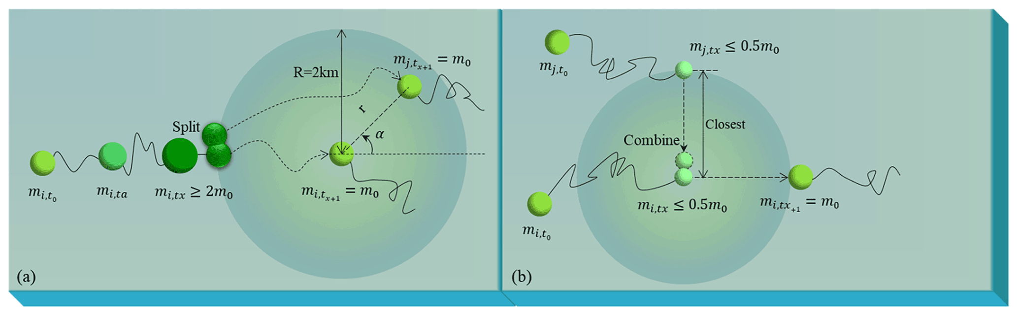
Figure 2Diagram of the replication (a) and extinction (b) process of simulated macroalgae represented by particles.
2.1 Model framework
The model system for FMGDM v1.0 consisted of a Lagrangian particle-tracking module and an ecological module for macroalgal growth and mortality (Fig. 1). The floating drift process is described by the Lagrangian tracking module, which is developed based on the FVCOM v4.3 offline Lagrangian tracking model (http://fvcom.smast.umassd.edu/, last access: 20 September 2020) (Chen et al., 2012, 2013, 2021) and driven by surface wind and ocean flows. By contrast, in the ecological module of macroalgae, the processes of dynamic growth and mortality in the floating state are exhibited by particle replication and disappearance, and either the growth or mortality rate of each simulated particle is dynamically determined by the temperature, irradiation, and nutrients where the floating particle is in space and time. The position, velocity, quantity, and represented biomass of particles are synchronously updated between the two modules. The physical and environmental factors are updated from the regional and local weather, ocean numerical model system, and marine atlas datasets. Based on the updated locations and biomasses of simulated particles, the coupled individual-based tracking and ecological model, applicable in the coverage and biomass simulation of floating macroalgae, is achieved.
2.2 Lagrangian particle-tracking module
Based on the hydrodynamic model, the Lagrangian particle-tracking module was established. The current velocity v is obtained by spatially and temporally interpolating the three-dimensional (3D) velocity field from the hydrodynamic model. Horizontal and vertical interpolations were carried out via bilinear interpolation. The 10 m height wind velocity Vw contributed to the movement of macroalgae floating at the sea surface. The windage coefficient κ was determined by the size of macroalgae and the floating depth on the sea. κ is assumed to be a fixed value, which does not change with the size of macroalgae in different life stages. The drifting velocity of floating macroalgae patches is determined using Eq. (1).
To ensure the accuracy of particle trajectory, Eq. (2) is integrated by the fourth-order Runge–Kutta algorithm (Chen et al., 2021), and the time step of calculation Δt is 60 s.
Dispersion, which was not caused by wind or currents, is also included in the trajectory tracking module. It mainly exhibited a stochastic movement, which was regarded as horizontal and vertical random walks by adding extra terms to particle trajectory calculation. Since the macroalgae mainly float at the sea surface without significant vertical migration, the vertical random walk was not turned on in the model setting. The horizontal random diffusion of the particles Δxr is considered in simulation as Eq. (3). The coefficient of horizontal random diffusion, Kr (unit: m2 s−1), and the time step for random diffusion was set to 6 s according to Visser's criterion. The unit vector a takes a random direction angle, and the random number R, fitted to a normal distribution, takes a value between 0 and 1.0.
Therefore, the final position of Lagrangian particle tracking during one-time step Δt can be expressed as
2.3 Ecological module
The ecological module reflects the growth and extinction of macroalgae by the replication and extinction of particles. One initial particle represented a patch with fixed biomass (m0) of floating macroalgae and the value could be adjusted according to needs. It was replicated and randomly released within a 2 km radius of the original location when the represented biomass of the particle exceeded 2m0. The biomass of the two particles returned to the initial value m0. Both particles then underwent drifting and growth or extinction processes independently (Fig. 2a). Additionally, when two nearby particles had biomass below 0.5m0, they were combined to form one particle with m0, representing the extinction process (Fig. 2b).
The macroalgae growth structure of this ecological module refers to the Ulva sp. growth models established by Ren et al. (2014) and Sun et al. (2020). The physiological process of this module is reflected in the absorption and loss of carbon (C), nitrogen (N), and phosphorus (P). Their uptake rates were represented as VC, VN, and VP, respectively. The loss rates were represented as LC, LN, and LP, respectively. The calculation of dynamic change in single-particle was expressed as
We expressed the biomass evolution as carbon. The fresh weight (FW) could be determined by
where KTOC indicates the conversion ratio between C and FW. Based on the physiological characteristics, the conversion value between C and FW was set as 8 mmol C g FW−1 (Sun et al., 2020).
The total biomass (Mt) of floating macroalgae throughout the domain can be determined by summing up the biomass of all active particles.
The uptake and loss of C, N, and P are controlled by the photosynthesis, respiration, and mortality processes, proportional to biomass. The absorption of C is dependent on the function of photosynthesis f(I), limited by the functions of temperature fp(T), nutrients f(N), and light attenuation of self-shading by macroalgae f(ρ).
where f(ρ) is the effect of self-shading and depends on the type of macroalgae and assembled density ρ (mol C m−2). The photosynthesis function f(I) indicates the relation between photosynthesis and irradiation I (Jassby and Platt, 1976).
where Pmax is the maximum photosynthetic rate and α is the photosynthetic efficiency. The changes in internal nutrient quotas have a significant impact on the physiological processes of macroalgae. The N quota (QN) and the P quota (QP) represented N:C and P:C, respectively (Ren et al., 2014). The relationship between nutrient quotas and photosynthesis is derived from Droop (1968). QNmin and QPmin are the minimum quota of N and P, respectively.
The nutrient uptake rate is controlled by the concentration of N and P and limited by the functions of temperature fp(T) and absorption attenuation caused by macroalgae accumulation f(ρ). The functions of nutrient uptake rate are derived from Lehman et al. (1975). The absorption of nutrients by macroalgae mainly considers dissolved inorganic nitrogen (DIN) and dissolved inorganic phosphate (DIP). The uptake rates of DIN and DIP are represented as VDIN and VDIP, respectively. They are calculated as
The maximum uptake rate of DIN and DIP are represented as VmDIN and VmDIP, respectively. The concentration of DIN and DIP are expressed as CDIN and CDIP, respectively. The half-saturation coefficient for DIN and DIP are represented as KDIN and KDIP, respectively (Sun et al., 2020). QNmax and QPmax are the maximum quota of N and P, respectively.
The C loss is contributed by respiration and mortality. The C loss of respiration depends on the temperature-related function fr(T). The C loss of mortality depends on the irradiance-related function f(I), the nutrients-related function f(N), and the temperature-related function fm(T). The temperature limitation functions fp(T), fr(T), and fm(T) correspond to photosynthesis, respiration, and mortality processes, respectively, where Rd is the dark respiration rate. When the temperature is unsuitable for the survival of macroalgae, fr(T) keeps to a minimum value indicating minimal respiration. The mortality process replaces photosynthesis as the dominant one under severe temperature and light intensity.
Similar to the loss of C, the uptake and loss of N and P are controlled by the respiration processes, and they are also proportional to biomass. The loss rate of C, N, and P can be calculated by
It should be noted that there is no interaction between this ecological module and the ocean numerical model system since this model is designed for offline computation, which is driven by the ocean model output of physical and ecosystem simulation.
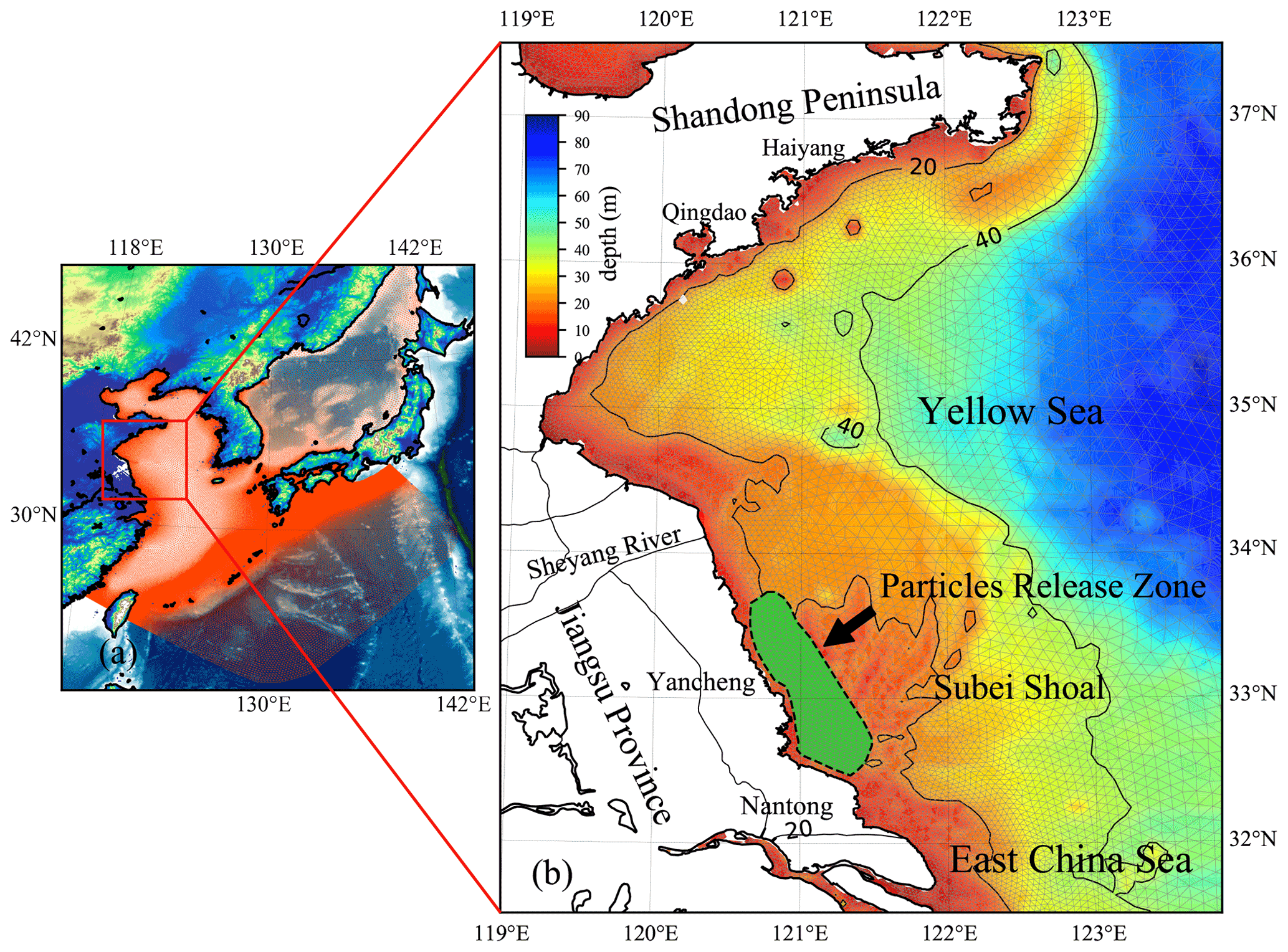
Figure 3(a) Location of the YS, China. The red mesh indicates the high-resolution triangle grids of ECS-FVCOM. (b) The enlarged view of the area and bathymetry bounded by the solid red line rectangle in panel (a). The green area surrounded by a black dotted line in the Subei Shoal indicates the initial release zone of simulated particles.
2.4 Study area
The first green tide in the YS broke out in 2007. Since then, it has become a recurrent phenomenon over the past 15 years (Keesing et al., 2011; Xiao et al., 2020). The major macroalgal species involved in the green tide has been identified as Ulva prolifera (Ding and Luan, 2009; Duan et al., 2011). In contrast with some macroalgae that only bloom in certain areas in coastal lagoons and estuaries, the green tide, accounting for most trans-regional macroalgal blooms worldwide (Liu et al., 2013), is much more complicated, both in spatial and temporal variations. The U. prolifera green tide in the YS primarily originates from the coast of Jiangsu Province, primarily the coast of Yancheng and Nantong, and can drift northward to the southern shore of the Shandong Peninsula and the coastal region of the Korean Peninsula (Liu et al., 2013; Son et al., 2012) (Fig. 3). Many loosely floating propagules of U. prolifera were provided from mid-April to mid-May every year (approximately 4000–6000 t), which could float and grow in the YS (Fan et al., 2015).
2.5 Data sources
2.5.1 Surface wind
The wind data at 10 derived from the surface wind dataset from the European Centre for Medium-Range Weather Forecasts (ECMWF) are available at https://www.ecmwf.int/en/forecasts/datasets/ (last access: 18 March 2019). The wind is interpolated to the triangular grids, covering the YS, East China Sea, Bohai Sea, and Japan Sea, in a spatial and temporal scale. The interpolated wind data were used as surface forcing for ECS (East China Sea)-FVCOM, with a spatial resolution of 0.125∘ and temporal resolution of 3 h.
2.5.2 Satellite data
The distribution area and density of the green tide can be estimated from satellite data (Hu et al., 2019; Qi et al., 2016). In this study, the green tide's spatial distribution and growth density were validated using satellite data. The Moderate Resolution Imaging Spectroradiometer with Terra sensor (MODIS-Terra) measured the green tide in the YS in 2014 and 2015, and the data are available from https://terra.nasa.gov/about/terra-instruments/modis (last access: 18 March 2019). In addition, the biomass quantified based on the satellite data from Hu et al. (2019) was used to verify the simulated U. prolifera biomass. Blocked by clouds, remote-sensing techniques exhibit difficulty in detecting small patches of floating macroalgae and often fail to capture the early status of the green tide (Garcia et al., 2013). In this study, only a few remote-sensing images can be used for result verification.
The remote-sensing dataset from https://www.ghrsst.org/ (last access: 2 January 2018), Group for High-Resolution Sea Surface Temperature (GHRSST), is used for data assimilation of sea surface temperature in the model system. The GHRSST dataset is based on daily values, with a spatial resolution of 0.01∘.
2.5.3 Drifting trajectory data
The drifting dataset used to evaluate the skills of the tracking module is composed of two parts: the trajectory data of satellite-tracked surface drifters released from the Subei Shoal in 2012 (Bao et al., 2015) and the subsurface drogue-drifter tracking data on the inner shelf of the ECS in 2017. The surface drifters contained four 40 cm wide, 70 cm high rectangular sails and a large central buoy (Bao et al., 2015). The subsurface drifter was constructed by a 67 cm diameter, 6 m high cylindrical subsurface sail and a 28 cm diameter central buoy.
2.5.4 Nutrient data
The seasonal nitrate and phosphate datasets of the YS were obtained from the 1∘ resolution World Ocean Atlas 2018 (Garcia et al., 2019) and merged with the datasets from the marine atlas of the YS (Wang et al., 1991). With these two datasets combined, the nutrients at the sea surface (April to August) were applied to this simulation through temporal interpolation.
2.6 Hydrodynamic model
An unstructured-grid FVCOM adapts to the second-order accurate discrete flux algorithm in an integral form to solve the governing equations on an unstructured triangular grid, which provides excellent mass and momentum conservation during the calculation (Chen et al., 2006, 2007, 2003; Ge et al., 2013). To better identify the ocean circulation along with the shelf break and deep ocean, the semi-implicit discretization, which could avoid the adjustment between two-dimensional external mode and three-dimensional internal mode, was applied. With this configuration, the ocean circulation as well as the astronomical tide around the ECS, YS, and adjacent regions could be reasonably determined (Chen et al., 2008; Ge et al., 2013). An integrated high-resolution numerical model system for the ECS (ECS-FVCOM) based on FVCOM v4.3 (http://fvcom.smast.umassd.edu/fvcom/, last access: 20 September 2020) was established and comprehensively validated using observational data (Chen et al., 2008; Ge et al., 2013). The high-resolution triangular grid of the ECS-FVCOM domain covers the YS, ECS, Bohai Sea, and Japan Sea, which have horizontal resolutions varying from 0.5–1.5 km in the estuary and coastal region, approximately 3 km in the path of the Kuroshio and 10–15 km along the lateral boundary in the North Pacific region (Fig. 3a). A total of 40 layers are considered in the vertical, including five uniform layers with a thickness of 2 m specified at the sea surface and bottom to resolve better surface heating and wind mixing and bottom boundary layer (Chen et al., 2008). The ocean bathymetry was retrieved and interpolated from ETOPO1 (https://ngdc.noaa.gov/mgg/global/global.html, last access: 18 March 2019). The initial temperature and salinity field and the volume transports along the open boundary of ECS-FVCOM were interpolated and retrieved from HYCOM (HYbrid Coordinate Ocean Model)+NCODA (Navy Coupled Ocean Data Assimilation) Global ∘ Analysis data (GLBA0.08), and eight major tide harmonic constituents (M2, S2, K2, N2, K1, O1, P1, and Q1), which are obtained from TPXO 7.2 Global Tidal Solution (Egbert and Erofeeva, 2002), were used along the open boundary (Ge et al., 2013). The freshwater discharge of the Yangtze River and Qiantang River (source: http://www.cjh.com.cn/, last access: 18 March 2019) was added to the upstream river boundary. Surface wind and radiations from the ECMWF were used in ECS-FVCOM as surface forces. In addition, the GHRSST dataset was applied to better determine the sea surface temperature using the model–data assimilation. The simulation time was set from March 29 to September 1, thus covering early spring to late summer. The water velocity, temperature, and salinity from ECS-FVCOM were fed into the FMGDM as input variables.
2.7 Model settings
Seven particle-tracking simulations were conducted. One hundred particles were released at a location that matched the drifter's in situ deployment position, and the horizontal random diffusion coefficient (Kr) was set as 50 m2 s−1. In addition, the depths for surface and subsurface drifters were set as 0.5 and 2 m, respectively. Thus, only half of the buoy was exposed above the sea surface for these drogue drifters, and the direct wind factor was not considered in the tacking simulations.
For the wind-exposed drifters floating at the sea surface, the wind drift is one of dominant contributions to transportation. Dagestad and Röhrs (2019) conducted drifting buoy experiments and found that windage accounted for 3 % of Stokes drift. Whiting et al. (2020) chose a constant 3 % coefficient in the free-floating macroalgal trajectory simulation. The setting of this coefficient was based on the debris drift simulation of the 2011 Japan tsunami (Maximenko et al., 2018). Additionally, Jones et al. (2016) reported that the horizontal movement of surface oil slicks is drifted by ∼ 3.5 % of the wind speed, including a 2 % direct wind drag and a 1.5 % wind speed adding to the surface Stokes drift (Abascal et al., 2009). The movements of free-floating macroalgae are influenced by wind and windage, which depend on the physical characteristics of drifters. The hydrodynamic surface layer had already accounted for wind movement, and the other wind drag for particle drift was composed of direct windage.
Based on the previous studies described above, the U. prolifera-induced total drifting windage was in a range of 2.7 %–3.5 %. A series of particle-tracking experiments were conducted in this windage range, with an interval of 0.1 %. Meanwhile, one experiment without the direct wind factor was also undertaken for reference. A total of 10 groups, with 1192 particles in every group, separated at a 0.02∘ horizontal resolution, were deployed in batches in the particle release zone (Fig. 3b) on 1 May 2014. These particles were traced for 120 d.
Most importantly, two realistic dynamic growth simulations were conducted. To verify the general applicability of the model, we simulated the growth and drift processes of U. prolifera in the YS in 2014 and 2015, respectively, with identical model configurations. In the two simulations, each particle represented 10 t biomass of floating U. prolifera, so that 4800 t were deployed initially. The initial coverage and biomass of the U. prolifera were determined based on the field surveys by Liu et al. (2013) and Q. Xu et al. (2014). The simulation time was 135 d from 16 April to 29 August. The initial particles are deployed continuously from 16 April to 15 May. Daily, 160 t biomass was spatially randomly released in the hot-spot zone (Fig. 3b) over an entire month. The horizontal random diffusion Kr was set as 200 m2 s−1 in the green tide simulation. In this study, instantaneous environmental factors, including temperature, nutrients, solar radiation intensity, ocean flow, and wind speed, were determined from the physical ECS-FVCOM model.
We set the parameters of the ecological module according to the physiological characteristics of U. prolifera. The functions of temperature were determined referring to the results of laboratory studies. U. prolifera has optimal photosynthesis efficiency at 20 ∘C and turns white and declines rapidly under high temperature and high light intensity (Cui et al., 2015; Song et al., 2015). When the temperature is suitable (5–25.7 ∘C), the temperature limitation of photosynthesis fp(T) and respiration fr(T) are consistent. When the temperature becomes unsuitable (< 5 ∘C or > 25.7 ∘C), the respiration of macroalgae, unlike photosynthesis, will remain at a lower level. When the high temperature exceeds a suitable situation (> 25.7 ∘C), the mortality process replaced photosynthesis as the dominant process.
According to the floating growth characteristics of U. prolifera, the self-shading limited function f(ρ) was determined. When the assembled density does not exceed 0.16 mol C m−2, the growth of U. prolifera is not restricted by self-shading. However, as the density increases, the accumulation of U. prolifera becomes significant and is at a maximum when the density is greater than 0.56 mol C m−2.
Table 1Parameters used in the ecological module for U. prolifera, modified from Sun et al. (2020).
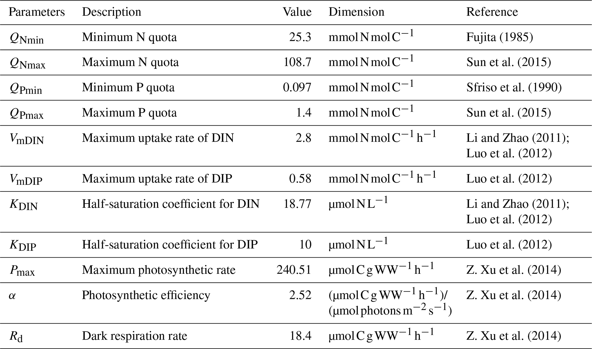
The complete list of parameters used in the ecological module of U. prolifera was shown in Table 1.
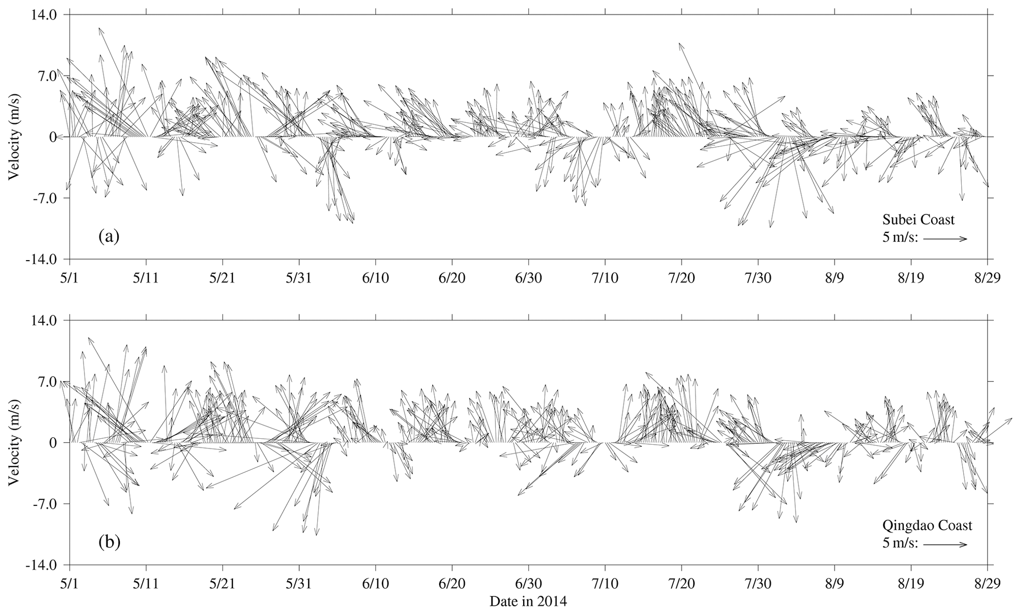
Figure 4Wind vectors at 10 m height near the Subei coast (a) and Qingdao coast (b) at a time interval of 6 h from May to August 2014.
3.1 Variations in environmental factors
3.1.1 Surface wind
The wind vectors at 10 m height near the Subei coast and the Qingdao coast, retrieved from ECMWF, are shown in Fig. 4. From May to July 2014, southerly and southeasterly winds prevailed in the coast of Subei and Qingdao, and the mean wind speed reached 5 m s−1. However, the southerly wind was stronger throughout May in Spring. In June, southeast winds blew significantly on the Subei coast, and the southerly wind still dominated the Qingdao coast; the wind speed was slightly lower than that in May. In August, the northeast wind was strengthened, especially from 1–10 August.
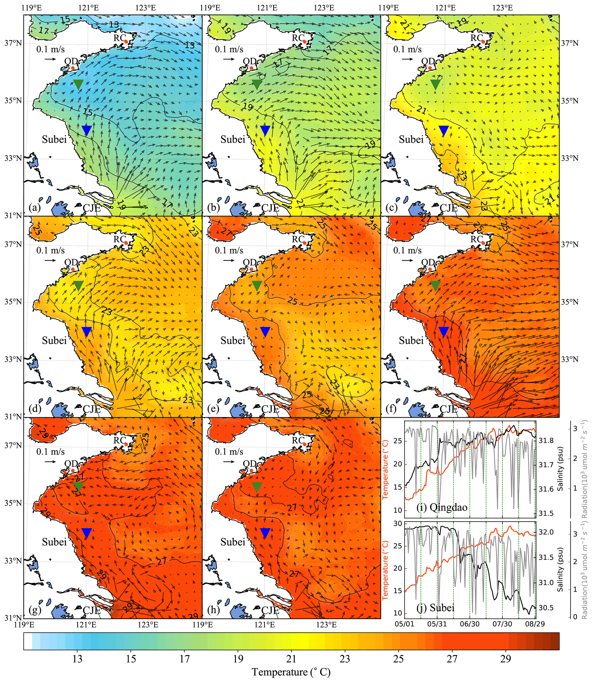
Figure 5Time-averaged distribution of surface current and temperature of every 15 d duration in 2014: (a) 1–15 May, (b) 16–30 May, (c) 31 May–14 June, (d) 15–29 June, (e) 30 June–14 July, (f) 15–29 July, (g) 30 July–13 August, (h) 14–29 August. The green and blue inverted triangles indicate the position of selected Qingdao (QD) coast and Subei offshore sites, respectively. Time series of surface temperature, salinity, and irradiation in Qingdao (i) and Subei (j).
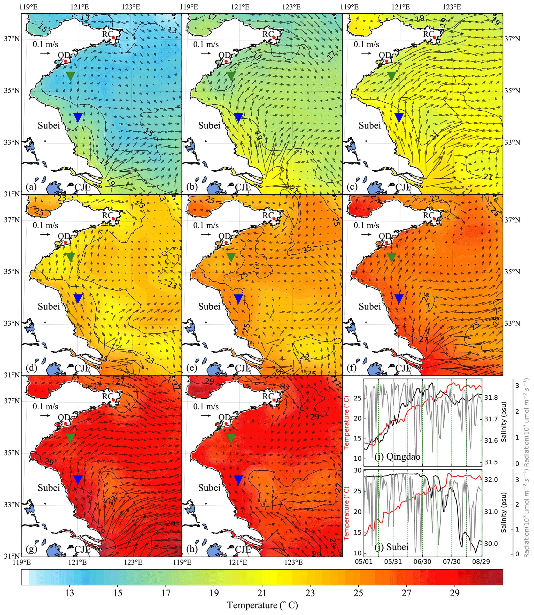
Figure 6Time-averaged distribution of surface current and temperature of every 15 d duration in 2015: (a) 1–15 May, (b) 16–30 May, (c) 31 May–14 June, (d) 15–29 June, (e) 30 June–14 July, (f) 15–29 July, (g) 30 July–13 August, (h) 14–29 August. The green and blue inverted triangles indicate the position of selected Qingdao (QD) coast and Subei offshore sites, respectively. Time series of surface temperature, salinity, and irradiation in Qingdao (i) and Subei (j).
3.1.2 Ocean circulation
The time-averaged distributions of surface ocean circulation every 15 d period in 2014 and 2015 are shown in Figs. 5 and 6, respectively. Affected by the southerly and southeasterly winds (Fig. 4), the coastal surface seawater flowed northward and was transported to the east of the south YS. This phenomenon was more pronounced in May, late June, and July (Fig. 5a, b, d, and f), indicating the possibility of U. prolifera drifting from the Subei Shoal toward the north. The same phenomenon was observed from May–June and early August of 2015 (Fig. 6a–d and g). Most of the time, surface seawater from the north YS was transported to the south YS through the east of Rongcheng (RC). In early June and July and August 2014 (Fig. 5c, e, g, and h), the surface seawater circulated counterclockwise in the middle region of the south YS. Simultaneously, the weak currents on the south side of the Shandong Peninsula may have caused U. prolifera to stay in this region and gradually land on the shore. Similar ocean circulations appeared in July and late August of 2015 (Fig. 6e, f, and h), and weak northward currents were observed in the Subei Shoal.
3.1.3 Temperature
Figures 5 and 6 also included the distribution of surface seawater temperature in 2014 and 2015, respectively, with every 15 d time averaging. The average temperature of the south YS reached 13 ∘C in May (Fig. 5a and b) and increased continuously in June (Fig. 5c and d). Surface seawater temperature along the Jiangsu coast and the East China Sea was generally 1–2 ∘C higher than that in other areas of the south YS. However, most of the south YS reached a high temperature, with over 25 ∘C, by July 2014 (Fig. 5e and f). From mid-July to the end of August, the surface temperature on the Jiangsu coast and parts of the Shandong Peninsula coast remained above 27 ∘C (Fig. 5f–h). The offshore sites of Qingdao and Subei were selected to determine the time series process for the physical factors (Figs. 5i and j and 6i and j). The surface temperatures of the two stations, the northern Jiangsu coast and Qingdao coast, were increased until they reached their peaks at the end of July with over 27 ∘C and remained until the end of August.
The distribution and tendency of south YS seawater temperature in 2015 (Fig. 6) were similar to those in 2014. However, compared with those in 2014, they had more extensive high-temperature coverage for the south YS in August 2015 (Fig. 6g and h). The surface temperature of most YS regions exceeded 27 ∘C, part of the Jiangsu coast even reached 29 ∘C. In addition, the surface temperatures of the two stations reached 25 ∘C in 2015, approximately 1 week later than they did in 2014 (Fig. 6i and j).
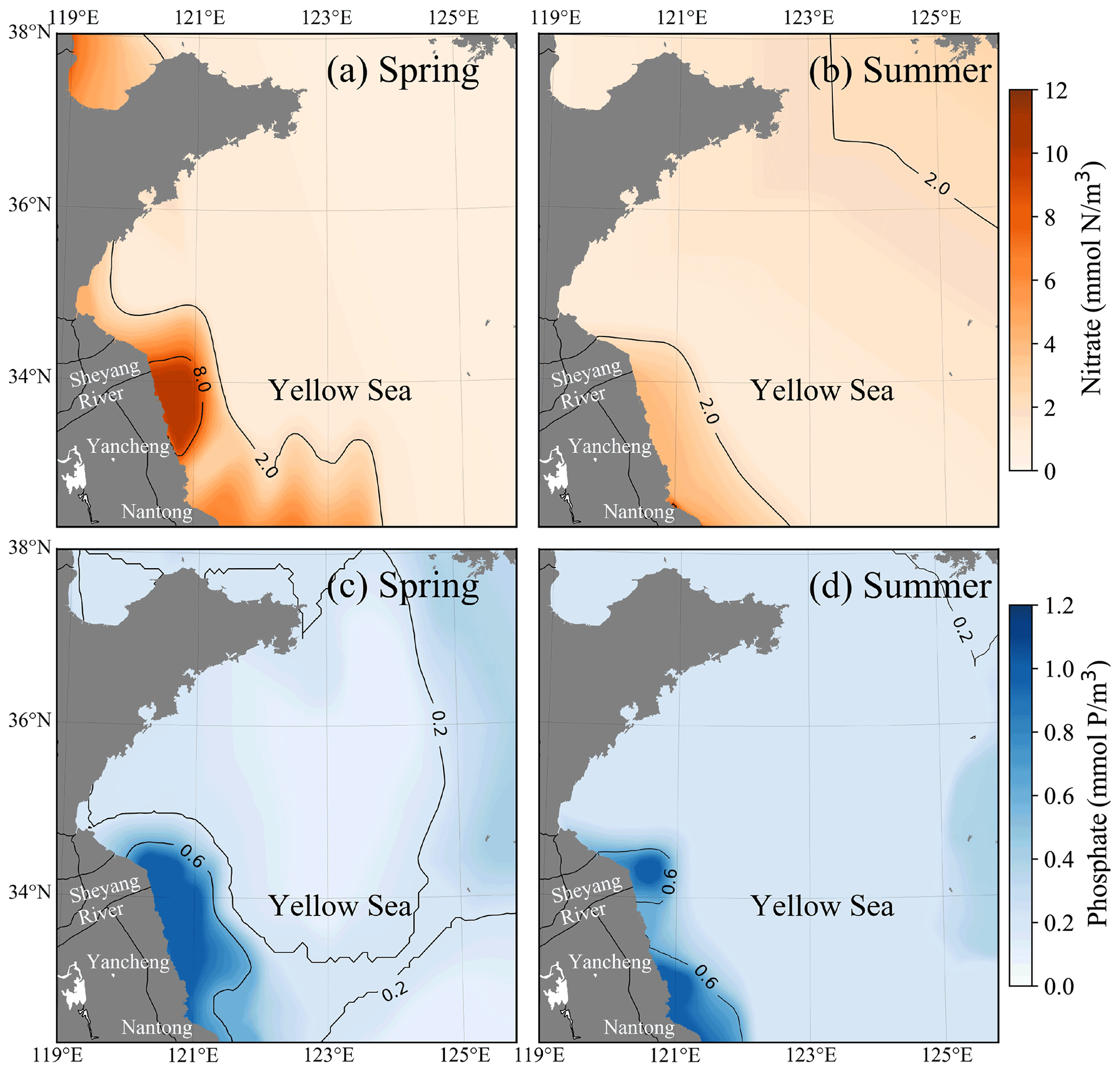
Figure 7Seasonally averaged surface distributions of nitrate (a, b) and phosphate (c, d) in the YS during spring (a, c) and summer (b, d).
3.1.4 Irradiation and salinity
Solar irradiation intensity is significantly different in the day and night. Therefore, only the irradiation intensity at noon was analyzed in Figs. 5i and j and 6i and j. Affected by the thickness of clouds, irradiation intensity at noon fluctuated drastically within 3200 . Compared with May and June, the irradiation intensity in July and August 2014 and 2015 decreased slightly.
The surface salinity of the south YS fluctuated between 29 and 33 PSU during the period of the green tide bloom (Figs. 5i and j and 6i and j), which was suitable for U. prolifera growth (Xiao et al., 2016). For this reason, the salinity limitation was ignored in the biological module.
3.1.5 Dissolved nutrients
The dissolved inorganic nutrients in the offshore region are mainly influenced by terrestrial sources, with prominent seasonal characteristics. The concentration of dissolved inorganic nutrients in the Jiangsu region was significantly higher than in other areas. The nitrate concentration in the offshore region of Jiangsu was generally above 2 mmol m−3 in spring (Fig. 7a) and summer (Fig. 7b), especially in the Yancheng region; the nitrate concentration was over 8 mmol m−3 in spring. The nitrate concentration in the other areas of YS, except the offshore region of Jiangsu, was mainly below 2 mmol m−3. The phosphate concentration in the offshore region of the Nantong and Sheyang River estuary was still high: more than 0.6 mmol m−3 in spring (Fig. 7c) and summer (Fig. 7d). In the north of the Yancheng offshore region, phosphate concentration decreased to ∼ 0.2 mmol m−3 in summer (Fig. 7d). In the central YS and south offshore area of the Shandong Peninsula, phosphate concentration was higher in summer (over 0.2 mmol m−3) than ∼ 0.1 mmol m−3 in spring.
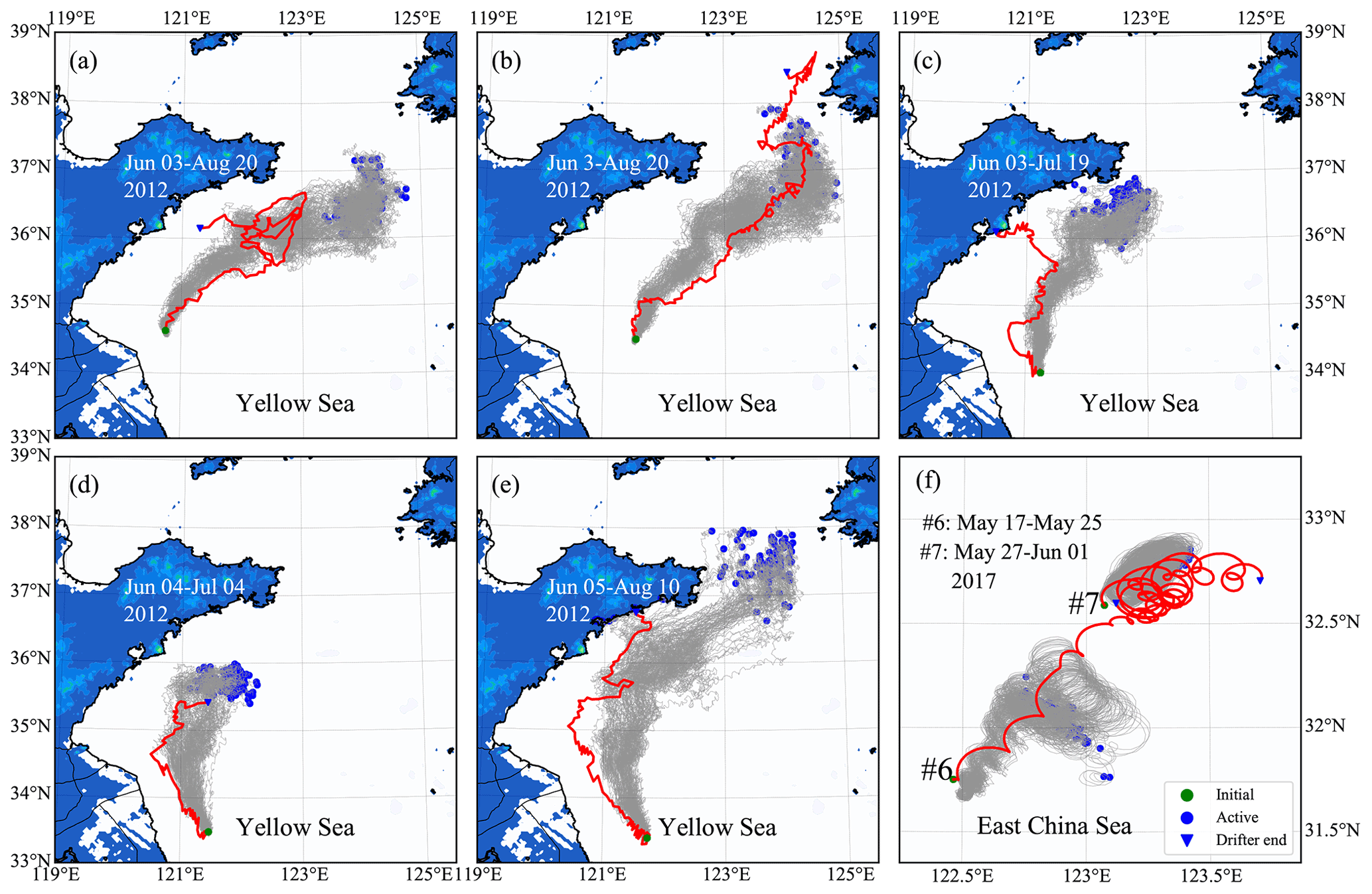
Figure 8Comparisons between observed (red lines) and simulated (gray lines) drifter trajectories. Panels (a)–(e) correspond to the drifters nos. 1–5, respectively. Panel (f) corresponds to drifters nos. 6–7.
3.2 Validation of tracking module
3.2.1 Tracking module evolution
The simulated particle trajectories are generally consistent with the observed drifter trajectories, particularly for a short-term prediction (Fig. 8). The tracking time for surface drifters nos. 1–5 lasted more than 1 month (Fig. 8a–e). The results show that the model was robust enough to reproduce the overall drifter's movement directions. Since the drifter paths may change with a great degree of randomness due to complex variations in ocean flow, winds, and waves, the long-term prediction of drifter paths and dispersal could be a great challenge. The tracking time for subsurface drifters nos. 6–7 (Fig. 8f) was relatively shorter: only 5–9 d. Compared with surface drifters, subsurface drifters were driven by a more complicated forcing relating to the extensive depth range of the sail. The water flow at a 2 m depth was selected as approximately the driving force, considering the average drifting state of subsurface drifters. The simulated trajectories were similar to the observed drifter's movement trends. However, the drifted distance was slightly shorter than the actual situation.
The model–data compression suggests that the particle-tracking algorithm in FMGDM can provide reasonable predictions for free-floating drifters with a higher confidence for surface drifters. In addition, the hydrodynamic model, ECS-FVCOM, is reliable. Our results showed that U. prolifera were mainly in a free-floating state at the sea surface.

Figure 9Evolution of the particle distribution in FMGDM tracking simulations. Colors indicate the different windage (2.7 %–3.5 %) of the simulated particles. The blue particles indicate the simulation without direct windage. (a) 5 June 2014; (b) 15 June 2014; (c) 30 June 2014; (d) 17 July 2014; (e) 28 July 2014; (f) 14 August 2014.
3.2.2 Windage simulation
The simulation results with different windages showed that particles first flowed northward and then turned northeastward (Fig. 9). With greater windage, the trend of northward transportation is more prominent. The particles with a windage of about 3.4 % could reach the southern coast of the Shandong Peninsula on 15 June (Fig. 9b) and then turned northeastward near 124∘30.00′ E (Fig. 9c and d). The particle group was split at the end of July. One part drifted northward continuously to 38∘ N and reached the North Korean coast, and the other was turned west (Fig. 9f). The particles with a windage coefficient of less than 3.2 % were stranded near the southern coast of the Shandong Peninsula in July and August (Fig. 9d–f). The particles without direct windage have significantly slow drifting, the northernmost nearly reaching the south coast of the Shandong Peninsula. Some particles moved northeastward to the center of the south YS. From the comparison, winds contributed significantly to the transport of free-floating drifters. The transport results with a 2.7 %–3.5 % windage range did not show a significant difference in the short-term simulation of 1–1.5 months (Fig. 9a–c). However, as the simulation time lasted longer, the transport pattern showed a noticeable difference (Fig. 9d–f). Compared with the evolution of green tides in the YS from remote sensing (Hu et al., 2019), it can be confirmed that the windage in a range of 3–3.2 % could be applied to the drift of green tide. In this study, 3.2 % was selected as the windage κ of the YS green tide simulation.
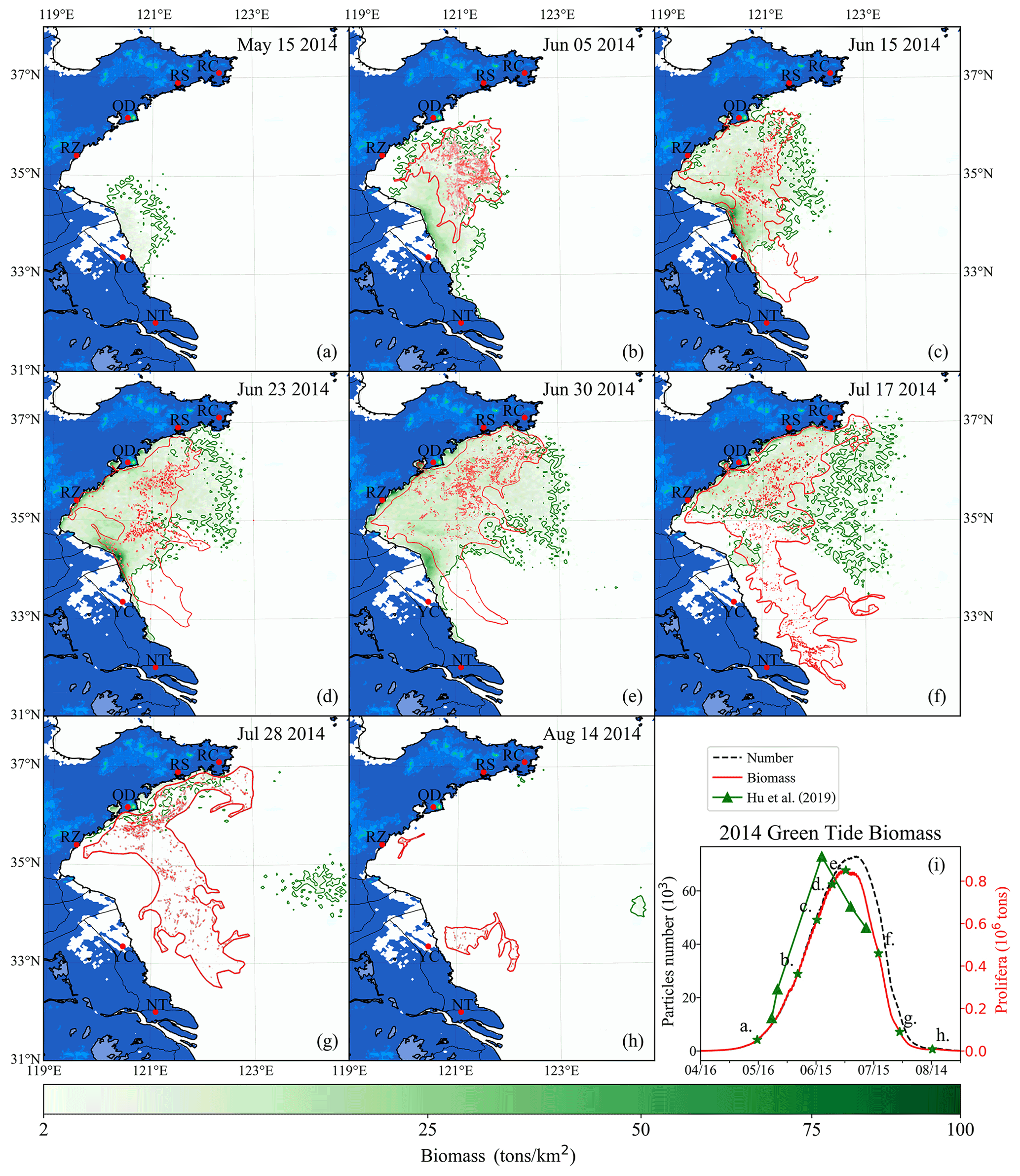
Figure 10Comparison between simulation and remote-sensing observation of green tides from May to August 2014 (a–h). The green image indicates the simulated biomass density of the green tide (color image, unit: t km−2). The red image shows the satellite-derived spatial coverage of U. prolifera from MODIS-Terra. Panel (i) is the time series of simulated biomass and particle number of green tides in 2014, compared with observed biomass from Hu et al. (2019). The green stars in panel (i) indicate the biomass of the corresponding date in panels (a)–(h).
3.3 Simulation of dynamic growth model
3.3.1 Spatiotemporal variation in U. prolifera
After being released into the Subei Shoal, the initial particles drifted and were dispersed by ocean flows and wind. The simulation result of the green tide in 2014 is shown in Fig. 10. It showed a small amount of U. prolifera floating on the Subei coast in mid-May (Fig. 10a). However, it was difficult to observe using remote-sensing technology in the early stage of green tide bloom. After 1 month of simulation, the modeling biomass increased to approximately 0.2×10⁶ t (Fig. 10i). Both observation and simulation showed that U. prolifera was transported northward and floated between the northern Jiangsu offshore region and the Shandong Peninsula (Fig. 10b). On 15 June (Fig. 10c), both the results of observation and simulation show that green tides had landed on the southern coast of the Shandong Peninsula, including the Rizhao (RZ) and Qingdao shore. Moreover, the observations show that the green tide bloomed around the coast of Nantong (NT) and Yancheng (YC), suggesting the continuous supply of additional U. prolifera from aquaculture rafts between May and June 2014. On 23 June (Fig. 10d), the result of both observation and simulation were consistent and showed that green tides had landed on the Shandong Peninsula on a large scale, and the farthest U. prolifera reached the Rushan (RS) coast. The entire coast and offshore regions were covered with a massive amount of floating U. prolifera. Due to the high concentration of nutrients, there were a large number of simulated particles growing at the Sheyang River estuary region in all of June. The biomass of the simulation reached a peak of 0.85×10⁶ t on 30 June, and the number of simulation particles reached approximately 71 000 (Fig. 10i). Subsequently, U. prolifera died out quickly, and its coverage decreased significantly. On 17 July (Fig. 10f), the floating U. prolifera still gathered on the south coast of the Shandong Peninsula. Different from the observation result, some small patches of the simulation result drifted eastward and reached 123∘ E.
In contrast with the simulation results, observation showed the re-occurrence of a large-scale green tide in the Yancheng and Nantong regions from 17 to 28 July (Fig. 10f and g), which, however, was uncaptured by the model. Both observation and simulation results showed that floating U. prolifera drifted eastward but still covered the south coast of the Shandong Peninsula at the end of July (Fig. 10g). After half a month, floating U. prolifera had died out (Fig. 10h). Observation shows that only the southern coast of Qingdao and the Subei Shoal had a few patches of U. prolifera on 14 August, which suggests there is still a possible U. prolifera source near the Subei Shoal even in the summertime in July and August. However, the U. prolifera of the simulation had almost vanished because the U. prolifera source was only initialized from mid-April to mid-May.
As there was no direct way of quantifying the floating U. prolifera biomass of green tides throughout the YS (Wang et al., 2018), the estimated biomass data of U. prolifera retrieved from remote-sensing observations (Hu et al., 2019) was adopted to validate the simulated biomass (Fig. 10i). The estimated biomass of U. prolifera rose rapidly and peaked with maximum values of 0.92×10⁶ t on 18 June 2014 (Hu et al., 2019). The biomass declined rapidly after reaching its peak, and U. prolifera almost died off at the end of July. Compared with observation results, the biomass of the simulation peaked after 12 d with a similar value. The growth trends between observation and simulation were similar. Considering the highly random dispersion as well as the dynamic life history of U. prolifera, our simulation provides reasonable modeling results of biomass and spatial coverage.
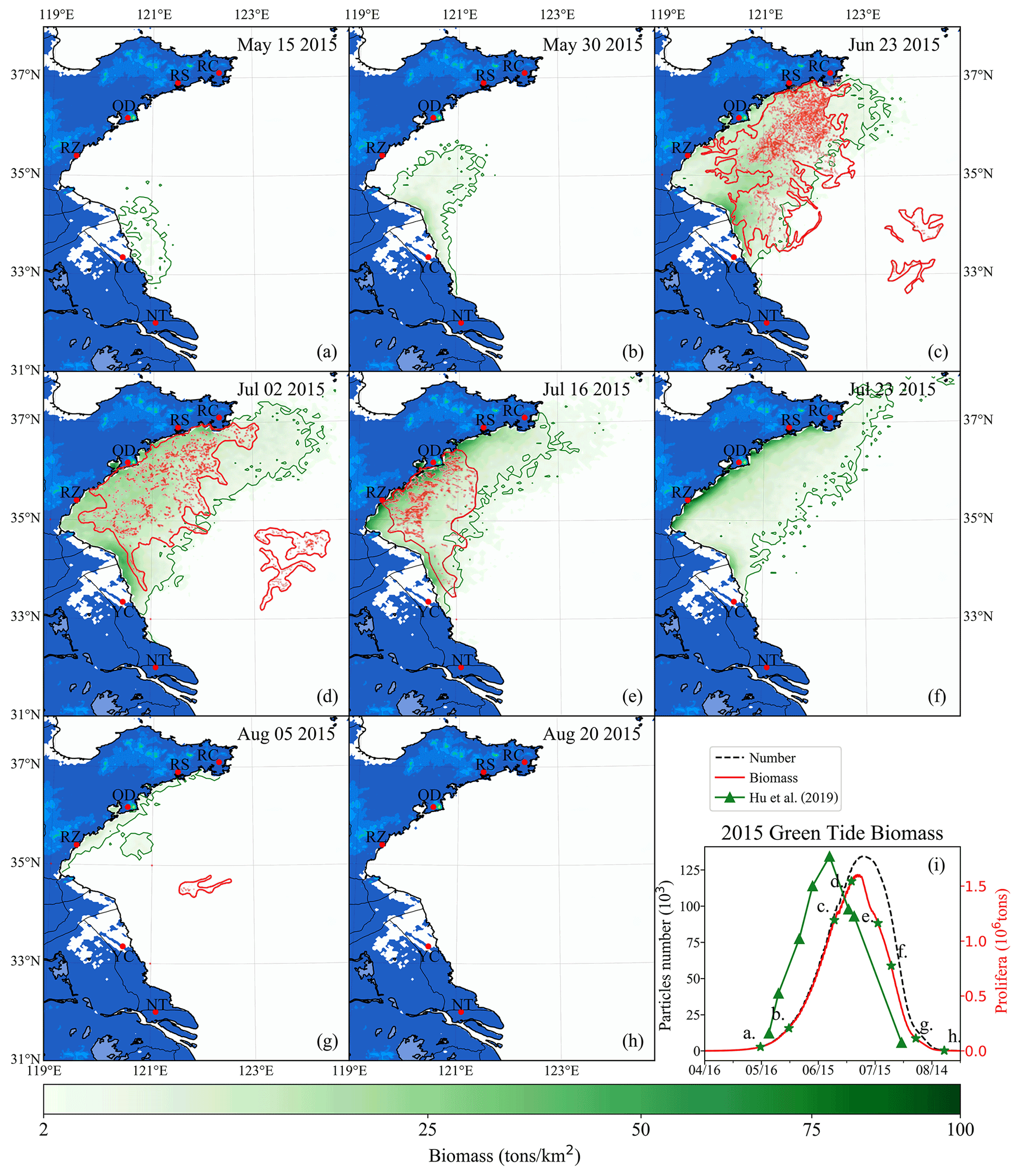
Figure 11Comparison between simulation and remote-sensing observation of green tides from May to August 2015 (a–h). The green image indicates the simulated biomass density of the green tide (color image, unit: t km−2). The red image shows the satellite-derived spatial coverage of U. prolifera from MODIS-Terra. Panel (i) is the time series of simulated biomass and particle number of green tides in 2015, compared with observed biomass from Hu et al. (2019). The green stars in panel (i) indicate the biomass of the corresponding date in panels (a)–(h).
To verify the reliability of the coupled model system, the green tide that bloomed in 2015 was also simulated and compared with the observations made. The simulation shows that a small amount of U. prolifera was floating near the coast of Jiangsu in mid-May (Fig. 11a). On 30 May, the coverage of floating U. prolifera increased, while the northernmost green tide patches were close to 35∘ N (Fig. 11b). On 23 June (Fig. 11c), both the results of observation and simulation showed that the green tide had entered the Shandong Peninsula with large-scale coverage, distributed in most of the seas from Subei to the Shandong Peninsula, and bloomed strongly offshore Qingdao to RS. On 2 July, both observation and simulation showed that the green tide was still gathered along the south coast of the Shandong Peninsula, and the northernmost part of the distribution range reached RC (Fig. 11d). In addition, observation showed scattered patches of U. prolifera floating in the center of the south YS from the 23 June to 2 July, which cannot be simulated. On 16 July (Fig. 11e), satellite observations showed that the coverage of green tide reduced considerably, and the distribution range had shrunk toward the west of 121∘30′E. In late July, the simulation result showed that the biomass declined rapidly; however, the green tides were still widely distributed in the southern regions of the Shandong Peninsula. On 5 August, observations showed small patches of the floating green tide in the middle of the south YS (Fig. 11g). In simulation results, a small amount of the green tide remained along the coast of the Shandong Peninsula. On 20 August (Fig. 11h), the green tide in the YS completely disappeared from satellite observation and numerical simulation. Comparing the biomass of observation and simulation, the estimated biomass of U. prolifera based on remote sensing peaked with maximum values of approximately 1.77×10⁶ t on 21 June 2014 (Hu et al., 2019), while the simulated biomass peaked after 13 d with a similar value of 1.6×10⁶. The number of simulation particles peaked at approximately 134 000 (Fig. 11i).
4.1 Uncertainties of physical, biological, and anthropic processes
The observation of the entire bloom process is technically complex in the study of massive floating macroalgal blooms. In this study, a floating macroalgal growth and drift model was established, supplemented by remote-sensing observations, which can reproduce the entire process and predict the development of macroalgal bloom. However, there are many uncertainties throughout the blooming process, which could significantly limit the precision of long-term prediction.
In the realistic numerical simulations of green tides from 2014 to 2015, the initial biomass of U. prolifera had the same configuration of 4800 t, deployed continuously from April 16 to May 15 based on the estimation in previous studies (Liu et al., 2013; Q. Xu et al., 2014). The initial distribution was also uniform. However, high uncertainties regarding the biomass and distribution were observed. The initial biomass of U. prolifera was determined primarily by the scale of local Porphyra aquaculture around the Subei coastal region and the timing of harvest activities. The precise estimation of initial biomass and timing requires extensive monitoring for these activities as well as robust and timely satellite assessment of satellite remote sensing.
From the satellite observations in June and July 2014, we observed stable patches of U. prolifera off the Subei Shoal (Fig. 10c–g), indicating the continuous supply of U. prolifera from the local Porphyra aquaculture activities in summer, resulting in stable bloom off the Subei Shoal and northward drift. Therefore, this factor, which could lead to significant bias of U. prolifera distribution and biomass, should be considered during long-term simulations.
During the green tide bloom, large-scale salvage operations were implemented to reduce the biomass of floating U. prolifera in Jiangsu and Shandong coastal waters (Liu et al., 2013; Wang et al., 2018), which could significantly change the local biomass. The biomass of salvage operations reaches 1.5–2.0 × 10⁶ t every spring and summer along the Shandong coastal region (Ye et al., 2011; Zhou et al., 2015), which could be the reason for the underestimation of biomass from 2–16 June 2015 (Fig. 10d and e). The salvage operations cause significant uncertainty for numerical prediction, particularly along the coast where the operations are primarily conducted.
The propagules are distributed near the floating Ulva with a high density and move with ocean flows (Li et al., 2017). The modified clay (MC) at a proper dose can flocculate with microscopic propagules and effectively remove microscopic propagules from the water column (Li et al., 2020). The physiological processes of Ulva cells could be disrupted by MC (Zhu et al., 2018). This method was frequently used to mitigate blooms in local areas (Li et al., 2017). The intervention of human activities on the blooming process was not considered in the model. Large-scale salvage and elimination activities play essential roles in reducing the scale and intensity of the green tide bloom. When the observed biomass peaked, the biomass in the simulation maintained an increasing trend. Finally, the maximum simulated biomass was similar to the maximum estimated biomass.
4.2 Short-term variations and quick response
To reduce the errors of long-term simulation, caused by the complex origin of initial floating macroalgae and the uncertainty of growth and drift, the time of each simulation was shortened by dividing the entire long-term simulation into multiple short-term simulations and renewed the location and biomass in every short-term modeling by the initialization of floating estimated by remote-sensing observation.
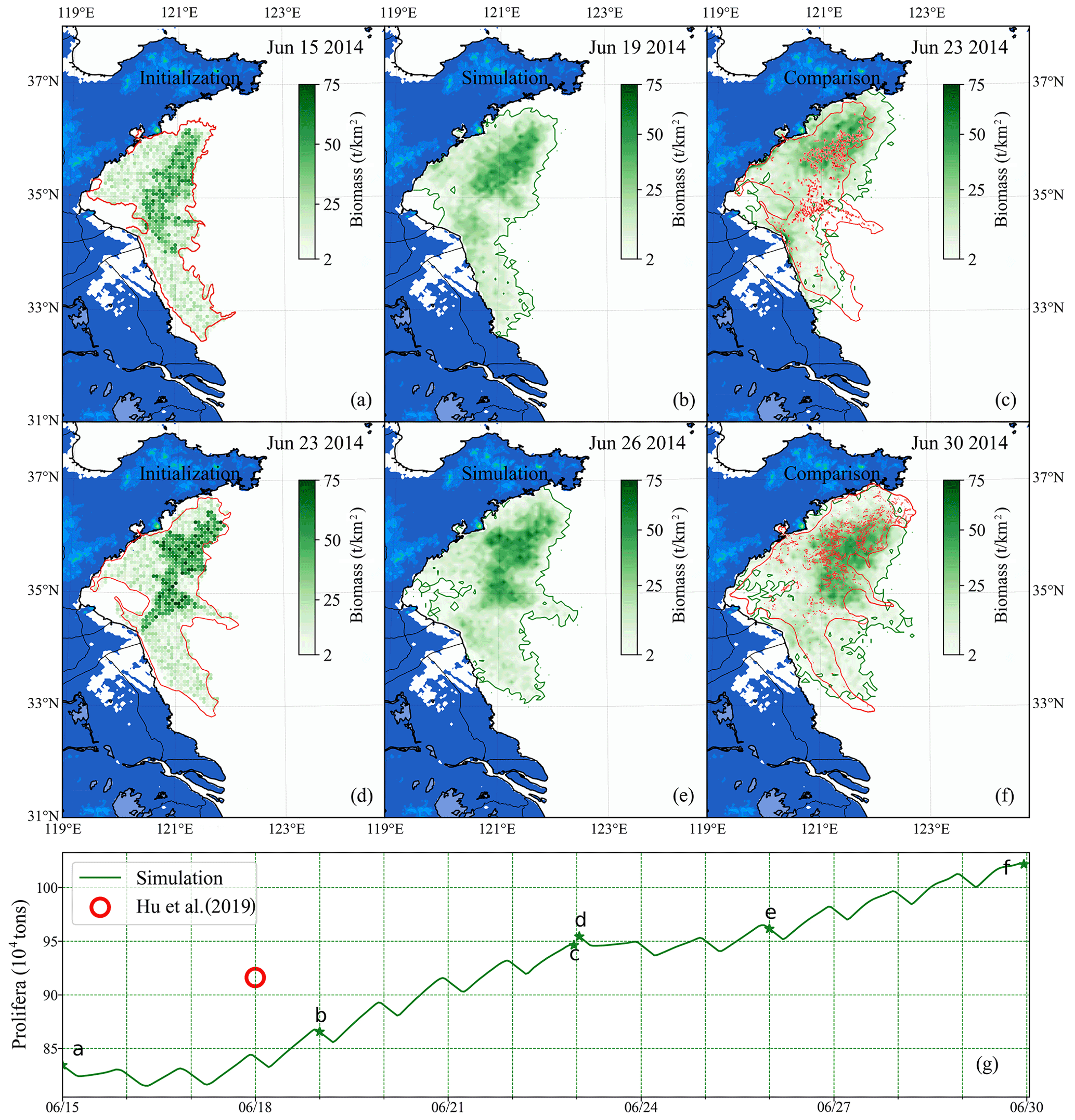
Figure 12Comparison of short-term simulation and satellite observation of green tides in 2014: position and distribution of green tide density released initially on 15 June (a) and 23 June (d) based on the satellite data and estimated biomass. Panels (b) and (e) are the modeling results of 19 June and 26 June, respectively. Panels (c) and (f) compare simulation and satellite observation on 23 and 30 June, respectively. The green image indicates the simulated result, and the red one indicates satellite observation. Panel (g) is the comparison of two consecutive simulated biomass (green line) and estimation biomass of satellite data (red circle). The green stars indicate the biomass of the corresponding date in panels (a)–(f).
Two consecutive simulations were carried out during the heyday of the YS green tide. One was configured for simulations from 15–23 June 2014 and the other from 23–30 June 2014. According to the distribution from remote-sensing observation and estimated biomass from Hu et al. (2019), the initial biomass and distribution of U. prolifera on 15 June 2014 was determined as shown in Fig. 12a and that on 23 June 2014 as in Fig. 12d. The initial biomass was approximately 0.83×10⁶ on 15 June and approximately 0.96×10⁶ on 23 June.
The time interval between two consecutive cloud-free satellite observations of green tides was generally large. Two intermediate results between the satellite observation gap were shown in Fig. 12b and e. After nearly 1 week of simulation, the coupled model system made a precise simulation, compared with remote sensing (Fig. 12c and f), and the biomass was similar to that estimated via satellite remote sensing (Fig. 12g). Moreover, spatial distribution was predicted well. Compared with long-term simulation, the variation in green tide distribution and biomass could be determined more accurately by the results of the short-term simulation. The accuracy of short-term simulations is reliable, and the short-term prediction of floating macroalgal blooms can be achieved by combining the numerical model with the satellite observations.
4.3 Roles of initial biomass and biotic and abiotic factors
The existence of diverse origins and continuous input of floating propagules significantly challenges the precise prediction and effective control of massive floating macroalgal blooms. In addition to the extensive provision from Porphyra aquaculture rafts in the Subei Shoal, the somatic cells, indicated by a laboratory study, could overwinter and restore growth in the annual spring bloom (Zhang et al., 2009), which is another significant source of U. prolifera. Additionally, four overwintering Ulva propagules that existed in sediments, including U. prolifera, may recover their growth when the temperature and irradiation are appropriate (Liu et al., 2012). Every April, before the occurrence of green tides, Ulva propagules are already widespread on the southern coast of the YS (Yuanzi et al., 2014). The transport trajectory was strongly affected by the origin of U. prolifera. Under the same environmental conditions, the scale of the bloom was determined primarily by the initial organisms. During the macroalgal bloom, the propagule supply from the coastal waters is continuously uncertain and difficult to determine through satellite observations or in situ surveys. Therefore, the feature that there was still large-scale U. prolifera distribution around the Subei Shoal in June and July 2014 has not yet been captured, as shown by satellite observations (Fig. 10), despite the continuous entering during the period of Porphyra aquaculture raft collection (mid-April to mid-May) having been considered in the green tide simulations.
The growth of floating macroalgae is affected by a variety of environmental factors. The influences of abiotic factors (e.g., temperature and irradiation) and biotic factors (e.g., nutrients) have been considered in the macroalgae growth module. Many macroalgae species have a clear thermo-period, which is sensitive to temperature. The changes in temperature in the surface layer of the water column in the YS has significant seasonal characteristics (Figs. 5 and 6). From spring to late summer, the temperature controls biological processes of the main species of YS green tides from germination, growth, and reproduction to extinction (Fan et al., 2015), which is reflected in the temporal dynamics of biomass (Figs. 10i and 11i). The photosynthesis is limited by light attenuation caused by self-shading and floating depth of macroalgae, which changes with the growth stage (Ren et al., 2014), and the module has not yet detailed this process. Meanwhile, the coastal turbid water that contains abundant suspended particulate matter can also limit the growth of green tide due to strong light attenuation in the upper surface water column. The initial release zone in the Subei Shoal is influenced by significant suspended sediment dynamics (Bian et al., 2013). Therefore, the growth rate in the coastal region in Jiangsu and Shandong is probably limited by suspended sediment.
Nutrient eutrophication frequently results in macroalgal blooms in coastal waters (Liu et al., 2013), which can also be reflected in the simulation results. There are significant differences in the concentration of dissolved nutrients between the coastal and offshore areas of the YS (Fig. 7). The simulation showed massive macroalgal bloom in the coastal area of Subei (34∘ N) in late June (Figs. 10c–e and 11c), which was directly related to the nutrient eutrophication here, with the dissolved nitrate about 8 mmol m−3 and the dissolved phosphate over 0.6 mmol m−3. The macroalgae growth in the offshore areas is relatively weaker because of nutrient limitation. The nutrient concentration is one of the major factors that influence spatial coverage of macroalgal bloom, and the abiotic factors including temperature and solar irradiation mainly modulate the temporal dynamics.
Due to the difficulty in obtaining the distribution and variations in observational or simulated nutrient datasets, the accuracy of macroalgae simulation was limited by the deviation of nutrient datasets. Floating U. prolifera can efficiently absorb nutrients (Luo et al., 2012), and the concentration of nutrients in the sea would decrease sharply when U. prolifera blooms dramatically, which may hinder the rapid growth of U. prolifera (Wang et al., 2019). When the green tide bloom reaches its peak with millions of tons of biomass or drifts to the regions far offshore, the dissolved nutrient concentration may be a significant growth limitation, even if the temperature and irradiation are still suitable for growth (Figs. 5 and 6). Due to lack of further research data on ecological relationships, some biotic factors (e.g., dissolved oxygen and potential biological competition against Sargassum) and abiotic factors (e.g., suspended particulate matter) are difficult to parameterize (Solidoro et al., 1997) and are therefore not considered in the physical–ecological coupled module.
4.3.1 Prospects on model development
No technique was identified for the precise quantification of the biomass of floating macroalgae (Sun et al., 2020). Most growth models only considered the environmental factors in a fixed station and disregarded the spatial variation in floating growth. The environmental factors vary significantly at different locations. Based on Lagrangian particle tracking, each particle was considered an independent simulation unit. The drift velocity and growth rate for that particle were obtained according to the natural environmental factors corresponding to the spatial position and time that particles locate. The simulation principle of this model is suitable for the actual situation of massive floating macroalgal blooms, which float and grow across vast regions.
The large-scale bloom of floating macroalgae affected the distribution of nutrients. The simulations in future studies should incorporate the circulation of nutrients between macroalgae and the ocean environment to improve the coupled model development at a more precise spatiotemporal scale. By coupling with the regional ecosystem or biogeochemical model, this model can be used to study the consumption of nutrients by the macroalgal blooms and its limitation on the growth of macroalgae. In particular, the model of floating U. prolifera could be established as a warning system of green tide disaster forecasting and be an efficient and economical tool for the prevention and management of green tides. Despite being used to simulate the green tide, this coupled model can also be applied to other large-scale macroalgae disasters that bloom in different parts of the world.
A system that coupled the ecological dynamic growth module with the physical drift module for macroalgae was developed to study the spatial and temporal variations in massive floating macroalgal bloom. The dynamic process of growth and drift is achieved by the replication/extinction and Lagrangian-based particle tracking. It was applied to the dynamic simulation of the YS green tide blooms in 2014 and 2015, with environmental drivers from ECS-FVCOM. The simulation results were verified against various observation data and demonstrated reasonable prediction precision. The modeling experiments also suggested that the surface wind played a crucial role in the northward drifting of U. prolifera from the Subei Shoal and finally resulted in an annual ecosystem disaster for the adjacent coastal region. The realistic simulation for 2 years exhibited many uncertainties from natural and human processes during the long duration from early spring to late summer, potentially leading to extensive prediction bias. However, the short-term simulation in this model, along with the determination of spatial coverage and biomass, proved to be an efficient and robust system for accurate forecasting of the development of U. prolifera.
Although this unique tool for macroalgae prediction was only applied in the simulation of the YS green tide, it can potentially be used to study other macroalgal blooms, such as golden tides caused by Sargassum, in other regions where sufficient information on the macroalgae physiological relationship with environmental factors are available.
The Fortran code of FMGDM v1.0 is available at https://doi.org/10.5281/zenodo.5067726 (Ge and Zhou, 2021a). The example of the green tide in the Yellow Sea, China, is available at https://doi.org/10.5281/zenodo.5067743 (Ge and Zhou, 2021b). The ECS-FVCOM forcing data (surface wind, radiations), the ocean bathymetry, and the results of ECS-FVCOM (water velocity, temperature, and nutrients), which are also used as input variables of FMGDM for the green tide simulation, the information initial particles position, the satellite pictures of the green tide in the YS 2014 and 2015, and the drifter trajectory dataset used to evaluate the tracking module are available at https://doi.org/10.5281/zenodo.5083889 (Ge and Zhou, 2021c).
Temporal and spatial dynamics of the Yellow Sea green tide bloom simulation in 2014: https://doi.org/10.5446/54438 (Zhou and Ge, 2021).
JG proposed and led this model development study. JG and FZ developed the coupled model. DL provided many important suggestions for this study and key data of U. prolifera growth. JG, PD, and CC contributed to the simulation result analysis of the ECS-FVCOM, which is used for this research. XW contributed to the remote-sensing interpretation. FZ processed the model outputs and wrote the paper with contributions from all co-authors.
The authors declare that they have no conflict of interest.
Publisher's note: Copernicus Publications remains neutral with regard to jurisdictional claims in published maps and institutional affiliations.
This research is supported by the National Natural Science Foundation of China (grant nos. 41776104, 41761144062) and the National Key R&D Program of China (grant nos. 2016YFC1402106, 2016YFA0600903).
This research has been supported by the National Natural Science Foundation of China (grant nos. 41776104 and 41761144062) and the National Key R&D Program of China (grant nos. 2016YFC1402106 and 2016YFA0600903).
This paper was edited by Andrew Yool and reviewed by Jonathan Whiting and two anonymous referees.
Abascal, A. J., Castanedo, S., Mendez, F. J., Medina, R., and Losada, I. J.: Calibration of a Lagrangian Transport Model Using Drifting Buoys Deployed during the Prestige Oil Spill, J. Coastal Res., 25, 80–90, https://doi.org/10.2112/07-0849.1, 2009.
Bao, M., Guan, W., Yang, Y., Cao, Z., and Chen, Q.: Drifting trajectories of green algae in the western Yellow Sea during the spring and summer of 2012, Estuarine, Coastal and Shelf Science, 163, 9–16, https://doi.org/10.1016/j.ecss.2015.02.009, 2015.
Bian, C., Jiang, W., Quan, Q., Wang, T., Greatbatch, R. J., and Li, W.: Distributions of suspended sediment concentration in the Yellow Sea and the East China Sea based on field surveys during the four seasons of 2011, J. Marine Syst., 121–122, 24–35, https://doi.org/10.1016/j.jmarsys.2013.03.013, 2013.
Brooks, M., Coles, V., Hood, R., and Gower, J.: Factors controlling the seasonal distribution of pelagic Sargassum, Mar. Ecol. Prog. Ser., 599, 1–18, https://doi.org/10.3354/meps12646, 2018.
Chen, C., Liu, H., and Beardsley, R. C.: An unstructured grid, finite-volume, three-dimensional, primitive equations ocean model: Application to coastal ocean and estuaries, J. Atmos. Ocean. Tech., 20, 159–186, https://doi.org/10.1175/1520-0426(2003)020<0159:AUGFVT>2.0.CO;2, 2003.
Chen, C., Beardsley, R. C., and Cowles, G.: An unstructured grid, finite-volume coastal ocean model (FVCOM) system, Special issue entitled “Advance in computational oceanography”, Oceanography, 19, 78–89, https://doi.org/10.5670/oceanog.2006.92, 2006.
Chen, C., Huang, H., Beardsley, R. C., Liu, H., Xu, Q., and Cowles, G.: A finite volume numerical approach for coastal ocean circulation studies: Comparisons with finite difference models, J. Geophys. Res.-Oceans, 112, C03018, https://doi.org/10.1029/2006JC003485, 2007.
Chen, C., Xue, P., Ding, P., Beardsley, R. C., Xu, Q., Mao, X., Gao, G., Qi, J., Li, C., Lin, H., Cowles, G., and Shi, M.: Physical mechanisms for the offshore detachment of the Changjiang Diluted Water in the East China Sea, J. Geophys. Res.-Oceans, 113, C02002, https://doi.org/10.1029/2006JC003994, 2008.
Chen, C., Limeburner, R., Gao, G., Xu, Q., Qi, J., Xue, P., Lai, Z., Lin, H., Beardsley, R., Owens, B., and Carlson, B.: FVCOM model estimate of the location of Air France 447, Ocean Dynam., 62, 943–952, https://doi.org/10.1007/s10236-012-0537-5, 2012.
Chen, C., Beardsley, R. C., Cowles, G., Qi, J., Lai, Z., Gao, G., Stuebe, D., Liu, H., Xu, Q., Xue, P., Ge, J., Ji, R., Hu, S., Tian, R., Huang, H., Wu, L., Lin, H., Sun, Y., and Zhao, L.: An unstructured-grid, finite-volume community ocean model FVCOM user manual, 4th edn., SMAST/UMASSD Technical Report-13-0701, University of Massachusetts, Dartmouth, 404 pp., available at: http://fvcom.smast.umassd.edu/fvcom/ (last access: September 2019), 2013.
Chen, C., Zhao, L., Gallager, S., Ji, R., He, P., Davis, C., Beardsley, R. C., Hart, D., Gentleman, W. C., Wang, L., Li, S., Lin, H., Stokesbury, K., and Bethoney, D.: Impact of larval behaviors on dispersal and connectivity of sea scallop larvae over the northeast U.S. shelf, Prog. Oceanogr., 195, 102604, https://doi.org/10.1016/j.pocean.2021.102604, 2021.
Cui, J., Zhang, J., Huo, Y., Zhou, L., Wu, Q., Chen, L., Yu, K., and He, P.: Adaptability of free-floating green tide algae in the Yellow Sea to variable temperature and light intensity, Mar. Pollut. Bull., 101, 660–666, https://doi.org/10.1016/j.marpolbul.2015.10.033, 2015.
Dagestad, K.-F. and Röhrs, J.: Prediction of ocean surface trajectories using satellite derived vs. modeled ocean currents, Remote Sens. Environ., 223, 130–142, https://doi.org/10.1016/j.rse.2019.01.001, 2019.
Ding, L. and Luan, R.: The taxonomy, habit and distribution of a green alga Enteromorpha prolifera (Ulvales, Chlorophyta), Oceanol Limnologia Sinica, 40, 68–71, 2009.
Droop, M. R.: Vitamin B12 and Marine Ecology. IV. The Kinetics of Uptake, Growth and Inhibition in Monochrysis Lutheri, J. Mar. Biol. Assoc. UK, 48, 689–733, https://doi.org/10.1017/s0025315400019238, 1968.
Duan, W., Guo, L., Sun, D., Zhu, S., Chen, X., Zhu, W., Xu, T., and Chen, C.: Morphological and molecular characterization of free-floating and attached green macroalgae Ulva spp. in the Yellow Sea of China, J. Appl. Phycol., 24, 97–108, https://doi.org/10.1007/s10811-011-9654-7, 2011.
Egbert, G. D. and Erofeeva, S. Y.: Efficient Inverse Modeling of Barotropic Ocean Tides, J. Atmos. Ocean. Tech., 19, 183–204, https://doi.org/10.1175/1520-0426(2002)019<0183:eimobo>2.0.co;2, 2002.
Fan, S., Fu, M., Wang, Z., Zhang, X., Song, W., Li, Y., Liu, G., Shi, X., Wang, X., and Zhu, M.: Temporal variation of green macroalgal assemblage on Porphyra aquaculture rafts in the Subei Shoal, China, Estuar. Coast. Shelf S., 163, 23–28, https://doi.org/10.1016/j.ecss.2015.03.016, 2015.
Fujita, R. M.: The role of nitrogen status in regulating transient ammonium uptake and nitrogen storage by macroalgae, J. Exp. Mar. Biol. Ecol., 92, 283–301, https://doi.org/10.1016/0022-0981(85)90100-5, 1985.
Garcia H. E., Weathers, K. W., Paver, C. R., Smolyar, I., Boyer, T. P., Locarnini, R. A., Zweng, M. M., Mishonov, A. V., Baranova, O. K., Seidov, D., and Reagan, J. R.: World Ocean Atlas 2018. Vol. 4: Dissolved Inorganic Nutrients (phosphate, nitrate and nitrate+nitrite, silicate), edited by: Mishonov, A., NOAA Atlas NESDIS 84, Silver Spring, MD, USA, 35 pp., available at: https://archimer.ifremer.fr/doc/00651/76336/, last access: July 2019.
Garcia, R. A., Fearns, P., Keesing, J. K., and Liu, D.: Quantification of floating macroalgae blooms using the scaled algae index, J. Geophys. Res.-Oceans, 118, 26–42, https://doi.org/10.1029/2012JC008292, 2013.
Ge, J. and Zhou, F.: Source code of Floating Macroalgal Growth and Drift Model (FMGDM_v1.0), Zenodo [code], https://doi.org/10.5281/zenodo.5067726, 2021a.
Ge, J. and Zhou, F.: Example for FMGDM_v1.0, application in the greet tides of the Yellow Sea, China, Zenodo [code], https://doi.org/10.5281/zenodo.5067743, 2021b.
Ge, J. and Zhou, F.: The ECS-FVCOM results and also the input variables of FMGDM, the initial particles, satellite pictures, and trajectories data, Zenodo [data set], https://doi.org/10.5281/zenodo.5083889, 2021c.
Ge, J., Ding, P., Chen, C., Hu, S., Fu, G., and Wu, L.: An integrated East China Sea-Changjiang Estuary model system with aim at resolving multi-scale regional-shelf-estuarine dynamics, Ocean Dynam., 63, 881–900, https://doi.org/10.1007/s10236-013-0631-3, 2013.
Gower, J. F. R. and King, S. A.: Distribution of floating Sargassum in the Gulf of Mexico and the Atlantic Ocean mapped using MERIS, Int. J. Remote Sens., 32, 1917–1929, https://doi.org/10.1080/01431161003639660, 2011.
Hu, L., Zeng, K., Hu, C., and He, M.: On the remote estimation of Ulva prolifera areal coverage and biomass, Remote Sens. Environ., 223, 194–207, https://doi.org/10.1016/j.ecss.2019.106329, 2019.
Jassby, A. D. and Platt, T.: Mathematical formulation of the relationship between photosynthesis and light for phytoplankton, Limnol. Oceanogr., 21, 540–547, https://doi.org/10.4319/lo.1976.21.4.0540, 1976.
Jones, C. E., Dagestad, K.-F., Breivik, Ø., Holt, B., Röhrs, J., Christensen, K. H., Espeseth, M., Brekke, C., and Skrunes, S.: Measurement and modeling of oil slick transport, J. Geophys. Res.-Oceans, 121, 7759–7775, https://doi.org/10.1002/2016jc012113, 2016.
Keesing, J. K., Liu, D., Fearns, P., and Garcia, R.: Inter- and intra-annual patterns of Ulva prolifera green tides in the Yellow Sea during 2007–2009, their origin and relationship to the expansion of coastal seaweed aquaculture in China, Mar. Pollut. Bull., 62, 1169–1182, https://doi.org/10.1016/j.marpolbul.2011.03.040, 2011.
Lee, J. H., Pang, I. C., Moon, I. J., and Ryu, J. H.: On physical factors that controlled the massive green tide occurrence along the southern coast of the Shandong Peninsula in 2008: A numerical study using a particle-tracking experiment, J. Geophys. Res.-Oceans, 116, C12036, https://doi.org/10.1029/2011JC007512, 2011.
Lehman, J. T., Botkin, D. B., and Likens, G. E.: The assumptions and rationales of a computer model of phytoplankton population dynamics1, Limnol. Oceanogr., 20, 343–364, https://doi.org/10.4319/lo.1975.20.3.0343, 1975.
Li, J. and Zhao, W.: Effects of nitrogen specification and culture method on growth of Enteromorpha prolifera, Chin. J. Oceanol. Limn., 29, 874–882, https://doi.org/10.1007/s00343-011-0516-6, 2011.
Li, J., Song, X., Zhang, Y., Pan, J., and Yu, Z.: An investigation of the space distribution of Ulva microscopic propagules and ship-based experiment of mitigation using modified clay, Mar. Pollut. Bull., 117, 247–254, https://doi.org/10.1016/j.marpolbul.2017.01.063, 2017.
Li, J., Song, X., Fan, X., and Yu, Z.: Flocculation of Ulva microscopic propagules using modified clay: a mesocosm experiment, Journal of Oceanology and Limnology, 38, 1283–1291, https://doi.org/10.1007/s00343-020-9348-6, 2020.
Liu, D., Keesing, J. K., Xing, Q., and Shi, P.: World's largest macroalgal bloom caused by expansion of seaweed aquaculture in China, Mar. Pollut. Bull., 58, 888–895, https://doi.org/10.1016/j.marpolbul.2009.01.013, 2009.
Liu, D., Keesing, J. K., He, P., Wang, Z., Shi, Y., and Wang, Y.: The world's largest macroalgal bloom in the Yellow Sea, China: Formation and implications, Estuar. Coast. Shelf S., 129, 2–10, https://doi.org/10.1016/j.ecss.2013.05.021, 2013.
Liu, F., Pang, S. J., Zhao, X. B., and Hu, C. M.: Quantitative, molecular and growth analyses of Ulva microscopic propagules in the coastal sediment of Jiangsu province where green tides initially occurred, Mar. Environ. Res., 74, 56–63, https://doi.org/10.1016/j.marenvres.2011.12.004, 2012.
Liu, X., Li, Y., Wang, Z., Zhang, Q., and Cai, X.: Cruise observation of Ulva prolifera bloom in the southern Yellow Sea, China, Estuar. Coast. Shelf S., 163, 17–22, https://doi.org/10.1016/j.ecss.2014.09.014, 2015.
Lovato, T., Ciavatta, S., Brigolin, D., Rubino, A., and Pastres, R.: Modelling dissolved oxygen and benthic algae dynamics in a coastal ecosystem by exploiting real-time monitoring data, Estuar. Coast. Shelf S., 119, 17–30, https://doi.org/10.1016/j.ecss.2012.12.025, 2013.
Luo, M., Liu, F., and Xu, Z.: Growth and nutrient uptake capacity of two co-occurring species, Ulva prolifera and Ulva linza, Aquat. Bot., 100, 18–24, https://doi.org/10.1016/j.aquabot.2012.03.006, 2012.
Lyons, D. A., Arvanitidis, C., Blight, A. J., Chatzinikolaou, E., Guy-Haim, T., Kotta, J., Orav-Kotta, H., Queirós, A. M., Rilov, G., Somerfield, P. J., and Crowe, T. P.: Macroalgal blooms alter community structure and primary productivity in marine ecosystems, Glob. Change Biol., 20, 2712–2724, https://doi.org/10.1111/gcb.12644, 2014.
Maximenko, N., Hafner, J., Kamachi, M., and Macfadyen, A.: Numerical simulations of debris drift from the Great Japan Tsunami of 2011 and their verification with observational reports, Mar. Pollut. Bull., 132, 5–25, https://doi.org/10.1016/j.marpolbul.2018.03.056, 2018.
Perrot, T., Rossi, N., Ménesguen, A., and Dumas, F.: Modelling green macroalgal blooms on the coasts of Brittany, France to enhance water quality management, J. Marine Syst., 132, 38–53, https://doi.org/10.1016/j.jmarsys.2013.12.010, 2014.
Putman, N. F., Goni, G. J., Gramer, L. J., Hu, C., Johns, E. M., Trinanes, J., and Wang, M.: Simulating transport pathways of pelagic Sargassum from the Equatorial Atlantic into the Caribbean Sea, Prog. Oceanogr., 165, 205–214, https://doi.org/10.1016/j.pocean.2018.06.009, 2018.
Qi, L., Hu, C., Xing, Q., and Shang, S.: Long-term trend of Ulva prolifera blooms in the western Yellow Sea, Harmful Algae, 58, 35–44, https://doi.org/10.1016/j.hal.2016.07.004, 2016.
Ren, J. S., Barr, N. G., Scheuer, K., Schiel, D. R., and Zeldis, J.: A dynamic growth model of macroalgae: Application in an estuary recovering from treated wastewater and earthquake-driven eutrophication, Estuar. Coast. Shelf S., 148, 59–69, https://doi.org/10.1016/j.ecss.2014.06.014, 2014.
Rothäusler, E., Gutow, L., and Thiel, M.: Floating Seaweeds and Their Communities, in: Seaweed Biology: Novel Insights into Ecophysiology, Ecology and Utilization, edited by: Wiencke, C. and Bischof, K., Springer Berlin Heidelberg, Berlin, Heidelberg, 2012.
Sfriso, A., Marcomini, A., Pavoni, B., and Orio, A. A.: Eutrofizzazione e macroalghe: la Laguna di Venezia come caso esemplare, Inquinamento, 4, 62–78, 1990.
Shi, X., Qi, M., Tang, H., and Han, X.: Spatial and temporal nutrient variations in the Yellow Sea and their effects on Ulva prolifera blooms, Estuar. Coast. Shelf S., 163, 36–43, https://doi.org/10.1016/j.ecss.2015.02.007, 2015.
Smetacek, V. and Zingone, A.: Green and golden seaweed tides on the rise, Nature, 504, 84–88, https://doi.org/10.1038/nature12860, 2013.
Solidoro, C., Pecenik, G., Pastres, R., Franco, D., and Dejak, C.: Modelling macroalgae (Ulva rigida) in the Venice lagoon: Model structure identification and first parameters estimation, Ecol. Model., 94, 191–206, https://doi.org/10.1016/s0304-3800(96)00025-7, 1997.
Son, Y. B., Min, J.-E., and Ryu, J.-H.: Detecting Massive Green Algae (Ulva prolifera) Blooms in the Yellow Sea and East China Sea using Geostationary Ocean Color Imager (GOCI) Data, Ocean Sci. J., 47, 359–375, https://doi.org/10.1007/s12601-012-0034-2, 2012.
Song, W., Peng, K., Xiao, J., Li, Y., Wang, Z., Liu, X., Fu, M., Fan, S., Zhu, M., and Li, R.: Effects of temperature on the germination of green algae micro-propagules in coastal waters of the Subei Shoal, China, Estuar. Coast. Shelf S., 163, 63–68, https://doi.org/10.1016/j.ecss.2014.08.007, 2015.
Sun, K., Ren, J. S., Bai, T., Zhang, J., Liu, Q., Wu, W., Zhao, Y., and Liu, Y.: A dynamic growth model of Ulva prolifera: Application in quantifying the biomass of green tides in the Yellow Sea, China, Ecol. Model., 428, 109072, https://doi.org/10.1016/j.ecolmodel.2020.109072, 2020.
Sun, K.-M., Li, R., Li, Y., Xin, M., Xiao, J., Wang, Z., Tang, X., and Pang, M.: Responses of Ulva prolifera to short-term nutrient enrichment under light and dark conditions, Estuar. Coast. Shelf S., 163, 56–62, https://doi.org/10.1016/j.ecss.2015.03.018, 2015.
Teichberg, M., Fox, S. E., Olsen, Y. S., Valiela, I., Martinetto, P., Iribarne, O., Muto, E. Y., Petti, M. A. V., Corbisier, T. N., Soto-JimÉNez, M., PÁEz-Osuna, F., Castro, P., Freitas, H., Zitelli, A., Cardinaletti, M., and Tagliapietra, D.: Eutrophication and macroalgal blooms in temperate and tropical coastal waters: nutrient enrichment experiments with Ulva spp, Glob. Change Biol., 16, 2624–2637, https://doi.org/10.1111/j.1365-2486.2009.02108.x, 2010.
Wang, C., Su, R., Guo, L., Yang, B., Zhang, Y., Zhang, L., Xu, H., Shi, W., and Wei, L.: Nutrient absorption by Ulva prolifera and the growth mechanism leading to green-tides, Estuar. Coast. Shelf S., 227, 106329, https://doi.org/10.1016/j.ecss.2019.106329, 2019.
Wang, M. and Hu, C.: Mapping and quantifying Sargassum distribution and coverage in the Central West Atlantic using MODIS observations, Remote Sens. Environ., 183, 350–367, https://doi.org/10.1016/j.rse.2016.04.019, 2016.
Wang, Y., Lu, S., Huang, S., Wang, Z., Liu, J., Wu, C., Wu, H., Chen, Y., Li, P., Zhang, S., Zhang, Z., Zhao, D., Tang, R., Jiang, G., and Tan, M.: Marine Atlas of Bohai Sea, Yellow Sea, East China Sea: Chemistry, China Ocean Press, Beijing, China, 1991.
Wang, Z., Fu, M., Xiao, J., Zhang, X., and Song, W.: Progress on the study of the Yellow Sea green tides caused by Ulva prolifera, Acta Oceanol. Sin., 40, 1–13, 2018.
Whiting, J. M., Wang, T., Yang, Z., Huesemann, M. H., Wolfram, P. J., Mumford, T. F., and Righi, D.: Simulating the Trajectory and Biomass Growth of Free-Floating Macroalgal Cultivation Platforms along the U.S. West Coast, Journal of Marine Science and Engineering, 8, 938, https://doi.org/10.3390/jmse8110938, 2020.
Xiao, J., Zhang, X., Gao, C., Jiang, M., Li, R., Wang, Z., Li, Y., Fan, S., and Zhang, X.: Effect of temperature, salinity and irradiance on growth and photosynthesis of Ulva prolifera, Acta Oceanol. Sin., 35, 114–121, https://doi.org/10.1007/s13131-016-0891-0, 2016.
Xiao, J., Wang, Z., Song, H., Fan, S., Yuan, C., Fu, M., Miao, X., Zhang, X., Su, R., and Hu, C.: An anomalous bi-macroalgal bloom caused by Ulva and Sargassum seaweeds during spring to summer of 2017 in the western Yellow Sea, China, Harmful Algae, 93, 101760, https://doi.org/10.1016/j.hal.2020.101760, 2020.
Xu, Q., Zhang, H., Ju, L., and Chen, M.: Interannual variability of Ulva prolifera blooms in the Yellow Sea, Int. J. Remote Sens., 35, 4099–4113, https://doi.org/10.1080/01431161.2014.916052, 2014.
Xu, Z., Wu, H., Zhan, D., Sun, F., Sun, J., and Wang, G.: Combined effects of light intensity and -enrichment on growth, pigmentation, and photosynthetic performance of Ulva prolifera (Chlorophyta), Chin. J. Oceanol. Limn., 32, 1016–1023, https://doi.org/10.1007/s00343-014-3332-y, 2014.
Ye, N., Zhang, X., Mao, Y., Liang, C., Xu, D., Zou, J., Zhuang, Z., and Wang, Q.: 'Green tides' are overwhelming the coastline of our blue planet: taking the world's largest example, Ecol. Res., 26, 477–485, https://doi.org/10.1007/s11284-011-0821-8, 2011.
Yuanzi, H., Liang, H., Hailong, W., Jianheng, Z., Jianjun, C., Xiwen, H., Kefeng, Y., Honghua, S., Peimin, H., and Dewen, D.: Abundance and distribution of Ulva microscopic propagules associated with a green tide in the southern coast of the Yellow Sea, Harmful Algae, 39, 357–364, https://doi.org/10.1016/j.hal.2014.09.008, 2014.
Zhang, X., Wang, H., Mao, Y., Liang, C., Zhuang, Z., Wang, Q., and Ye, N.: Somatic cells serve as a potential propagule bank of Enteromorpha prolifera forming a green tide in the Yellow Sea, China, J. Appl. Phycol., 22, 173–180, https://doi.org/10.1007/s10811-009-9437-6, 2009.
Zhou, F. and Ge, J.: green tide, TIB AV-Portal, https://doi.org/10.5446/54438, 2021.
Zhou, M., Liu, D., Anderson, D. M., and Valiela, I.: Introduction to the Special Issue on green tides in the Yellow Sea, Estuar. Coast. Shelf S., 163, 3–8, https://doi.org/10.1016/j.ecss.2015.06.023, 2015.
Zhu, J., Yu, Z., He, L., Cao, X., Liu, S., and Song, X.: Molecular Mechanism of Modified Clay Controlling the Brown Tide Organism Aureococcus anophagefferens Revealed by Transcriptome Analysis, Environ. Sci. Technol., 52, 7006–7014, https://doi.org/10.1021/acs.est.7b05172, 2018.