the Creative Commons Attribution 4.0 License.
the Creative Commons Attribution 4.0 License.
 | 27 Jan 2021
A simplified atmospheric boundary layer model for an improved representation of air–sea interactions in eddying oceanic models: implementation and first evaluation in NEMO (4.0)
Florian Lemarié
Guillaume Samson
Jean-Luc Redelsperger
Hervé Giordani
Théo Brivoal
Gurvan Madec
A simplified model of the atmospheric boundary layer (ABL) of intermediate complexity between a bulk parameterization and a three-dimensional atmospheric model is developed and integrated to the Nucleus for European Modelling of the Ocean (NEMO) general circulation model. An objective in the derivation of such a simplified model, called ABL1d, is to reach an apt representation in ocean-only numerical simulations of some of the key processes associated with air–sea interactions at the characteristic scales of the oceanic mesoscale. In this paper we describe the formulation of the ABL1d model and the strategy to constrain this model with large-scale atmospheric data available from reanalysis or real-time forecasts. A particular emphasis is on the appropriate choice and calibration of a turbulent closure scheme for the atmospheric boundary layer. This is a key ingredient to properly represent the air–sea interaction processes of interest. We also provide a detailed description of the NEMO-ABL1d coupling infrastructure and its computational efficiency. The resulting simplified model is then tested for several boundary-layer regimes relevant to either ocean–atmosphere or sea-ice–atmosphere coupling. The coupled system is also tested with a realistic 0.25∘ resolution global configuration. The numerical results are evaluated using standard metrics from the literature to quantify the wind–sea-surface-temperature (a.k.a. thermal feedback effect), wind–current (a.k.a. current feedback effect), and ABL–sea-ice couplings. With respect to these metrics, our results show very good agreement with observations and fully coupled ocean–atmosphere models for a computational overhead of about 9 % in terms of elapsed time compared to standard uncoupled simulations. This moderate overhead, largely due to I/O operations, leaves room for further improvement to relax the assumption of horizontal homogeneity behind ABL1d and thus to further improve the realism of the coupling while keeping the flexibility of ocean-only modeling.
- Article
(9817 KB) - Full-text XML
- BibTeX
- EndNote


Owing to advances in computational power, global oceanic models used for research or operational purposes are now configured with increasingly higher horizontal and vertical resolution, thus resolving the baroclinic deformation radius in the tropics (e.g., Deshayes et al., 2013; Metzger et al., 2014; von Schuckmann et al., 2018). Meanwhile fine-scale local models are routinely used to simulate submesoscales, which occur on scales on the order of 0.1–20 km horizontally, and their impact on larger scales (e.g., Marchesiello et al., 2011; McWilliams et al., 2019). By increasing the oceanic model resolution, small-scale features are explicitly resolved, but an apt representation of the associated processes also requires the relevant scales to be present in the surface forcings including the proper interaction with the low-level atmosphere.
1.1 Historical context
Historically, oceanic general circulation models (OGCMs) were forced by specified wind stress and thermal boundary conditions (from observations or reanalysis) independent from the oceanic state, thus often leading to important drifts in model sea surface properties. To minimize such drifts, a flux correction in the form of a restoration of sea-surface temperature and salinity toward climatological values can be added (e.g., Haney, 1971; Barnier et al., 1995). To overcome the shortcomings of the forcing with specified flux, Takano et al. (1973) proposed to use a parameterization of the atmospheric surface layer (ASL) constrained by large-scale meteorological data and by the sea state (essentially the sea-surface temperature and sometimes the surface currents) to compute the turbulent components of air–sea fluxes. Currently, whatever the target applications, such a technique is widely used in the absence of a concurrently running atmospheric model. Such parameterization of the ASL (known as bulk parameterization, e.g., Beljaars, 1995; Large, 2006), which corresponds to a generalization of the classical neutral wall law to stratified conditions (Monin and Obukhov, 1954), is expected to be valid in the first few tens of meters in the atmosphere. In practice, unless a fully coupled ocean–atmosphere model is used, atmospheric quantities at 10 m, either from existing numerical simulations of the atmosphere or from observations, are prescribed as input to the bulk parameterization. Throughout the paper, this approach will be referred to as “ASL forcing strategy”. A problem with such methodology is that the fast component of the system (the atmosphere) is specified to force the slow component (the ocean), whereas the inertia is in the latter. Indeed, a change in wind stress or heat flux will affect 10 m winds and temperature more strongly than sea surface currents and temperature. In the “ASL forcing strategy”, the key marine atmospheric boundary layer (MABL) processes are not taken into account, and thus feedback loops between the MABL and the upper ocean are not represented.
1.2 Air–sea interactions at oceanic mesoscales
An increasing number of studies based either on observational studies and/or on air–sea coupled simulations have unambiguously shown the existence of air–sea interactions at oceanic mesoscales (e.g., Giordani et al., 1998; Bourras et al., 2004; Chelton and Xie, 2010; Frenger et al., 2013; Schneider and Qiu, 2015; Oerder et al., 2016). Those interactions affect the mass, heat, and momentum exchange between the atmosphere and the ocean. We focus in this work on the dynamical response of the surface wind stress to the sea-surface properties (sea surface temperature (SST) and currents) which directly affects low-level winds, temperature, and humidity. Several mechanisms responsible for the surface wind-stress response to SST and oceanic currents can be invoked:
- i.
Downward momentum mixing. SST-induced changes in the stratification produce significant changes of wind speed and turbulent fluxes throughout the MABL with an increase (decrease) in wind speed over warm water (cold water). As the wind blows over warm water, the MABL becomes more unstable, which leads to an increased vertical mixing, resulting in a downward mixing of momentum from the upper atmosphere to the surface strengthening surface winds on the warm side of an SST front (e.g., Wallace et al., 1989). This mechanism results in a proportional relationship between wind-stress intensity and SST mesoscale anomalies which has been identified in observations and coupled simulations (e.g., O'Neill et al., 2010; Oerder et al., 2016). Considering spatial derivatives of this proportional relationship leads to a correlation between wind-stress divergence (curl) and downwind (crosswind) SST–gradient (e.g., Chelton and Xie, 2010; Schneider and Qiu, 2015).
- ii.
Atmospheric pressure adjustment. This mechanism corresponds to an adjustment of the atmospheric pressure gradient to the underlying SST, which manifests itself as a linear relation between horizontal wind divergence and the Laplacian of SST (Lindzen and Nigam, 1987; Minobe et al., 2008; Lambaerts et al., 2013).
- iii.
Oceanic current feedback. The momentum exchange between the ocean and the atmosphere is also largely affected by a dynamical coupling through the dependence of surface wind stress on oceanic surface currents (e.g., Dewar and Flierl, 1987). This coupling results in a drag exerted by the air–sea interface on the ocean which leads to a systematic reduction of the wind power input to the oceanic circulation.
Even if these three mechanisms are mainly active at oceanic eddy scales, they can induce significant effects at larger scales in regions with large SST gradients and/or surface currents (Hogg et al., 2009; Bryan et al., 2010; Renault et al., 2016a). They jointly leave their imprint on the wind divergence, and identifying the relative importance of each mechanism on the momentum balance is difficult because it depends on the dynamical regime and on the spatial and temporal scales of interest (Schneider and Qiu, 2015; Ayet and Redelsperger, 2019).
In the ASL coupling strategy the pressure adjustment mechanism is absent, and only a small fraction of the downward momentum mixing mechanism is accounted for through the modification of the surface drag coefficient depending on the ASL stability (Businger and Shaw, 1984; Chelton and Xie, 2010). As far as the current feedback is concerned, Renault et al. (2016b) showed that the reduction of wind power input to the ocean is systematically overestimated in oceanic simulations based on an ASL forcing strategy compared to air–sea coupled simulations. A simulation that neglects the MABL adjustment to the current feedback cannot represent the partial re-energization of the ocean by the atmosphere and hence overestimates the drag effect by more than 30 % (e.g., Renault et al., 2016b, 2019a). The ASL forcing strategy used in most oceanic models will thus overestimate the current feedback effect and underestimate the downward momentum mixing.
1.3 The proposed approach and focus for this paper
The various aspects discussed so far suggest that a relevant coupling at the characteristic scales of the oceanic mesoscales requires nearly the same horizontal resolution in the ocean and the atmosphere (since the atmosphere must “see” oceanic eddies and fronts) as well as an atmospheric component more complete than a simple ASL parameterization to estimate air–sea fluxes. This assessment raises numerous questions on current practices to force oceanic models across all scales1 in the absence of an interactive atmospheric model. The computational cost associated with the systematic use of fully coupled ocean–atmosphere models of similar horizontal resolution is generally unaffordable and comes with practical issues like the proper definition of initial conditions via data assimilation techniques (e.g., Mulholland et al., 2015) and the proper choice of a parameterization set. Moreover, in the fully coupled case at basin or global interannual scales the temporal consistency with the observed variability is generally lost unless a nudging toward observations or reanalysis is done in the atmosphere above the MABL (e.g., Bielli et al., 2009). There is thus clearly room for improvement in the methodology to compute the surface boundary conditions for an ocean model. Alternatives to the ASL forcing strategy have already been suggested by Kleeman and Power (1995), Seager et al. (1995), and Deremble et al. (2013). They proposed a vertically integrated thermodynamically active and dynamically passive MABL model where the wind and the MABL height are specified as in the current practices. Such a model allows a better feedback between SSTs and low-level air temperature and humidity because the latter two are prognostic (Abel, 2018). However, by construction, such models do not reproduce the various aforementioned coupling mechanisms affecting the surface wind stress. Their focus is on the improvement of the large-scale thermodynamics while ours is on the improvement of the eddy-scale momentum exchanges. In the present study we propose an alternative methodology to improve the representation of the downward momentum mixing and of the current feedback effect in ocean-only simulations, leaving aside the pressure gradient adjustment from now on. Our aim is to account for the modulation of atmospheric turbulence by anomalies in sea-surface properties in the air–sea flux computation, which is thought to be the main coupling mechanism at the characteristic scales of the oceanic mesoscales. As a step forward beyond the ASL forcing strategy we propose to complement the ASL parameterization with an ABL parameterization while keeping a single-column frame. By construction our approach excludes horizontal advection whose effect can be important in the vicinity of strong SST fronts (e.g., Kilpatrick et al., 2014; Ayet and Redelsperger, 2019). However, we considered that finding a simple and efficient MABL parameterization is the top priority to start investigating the viability of our approach in terms of practical implementation and computational cost. Indeed there exists a large variety of parameterization schemes to represent the effects of subgrid-scale turbulent mixing in the ABL (see LeMone et al., 2019, and references therein). The schemes based on a diagnostic or prognostic turbulent kinetic energy (TKE) are very popular for operational and research purposes despite well-identified shortcomings (e.g., Baklanov et al., 2011). For our purposes we do not need the full complexity of the schemes used in practice in atmospheric models because aspects like cloud processes and complex terrains are outside our scope. For this reason, the guideline in this paper is the development and the testing of a simplified version of the TKE-based scheme proposed by Cuxart et al. (2000) for over-water and over-sea-ice conditions. Note that the single-column approximation for our simplified model selected in this study is only a temporary choice to provide evidence on the viability of the whole approach. More advanced formulations allowing a more realistic momentum balance (i.e., including advection) to be recovered will be studied in future work.
1.4 Content
The objective of the present study is to introduce a simplified model of the MABL of intermediate complexity between a bulk parameterization and a full three-dimensional atmospheric model and to describe its integration to the Nucleus for European Modelling of the Ocean (NEMO) general circulation model (Madec, 2012). This approach will be referred to as the “ABL coupling strategy”. A constraint in the conception of such a simplified model is to allow an apt representation of the downward momentum mixing mechanism and partial re-energization of the ocean by the atmosphere while keeping the computational efficiency and flexibility inherent to ocean-only modeling. The paper is organized as follows. In Sect. 2, we describe the continuous formulation of the simplified model called ABL1d, including the parameterization scheme used to represent vertical turbulent mixing in the MABL and the strategy to constrain this model with large-scale atmospheric conditions. Section 3 provides the description of the dicretization and of the practical implementation of the ABL1d model in the NEMO framework. In Sects. 4 and 5 numerical results obtained for some atmosphere-only simplified test cases available in the literature and for a coupled NEMO-ABL1d simulation in a global configuration are shown. Finally, our conclusions and perspectives are summarized and discussed in Sect. 6.
In this section we first provide some basic elements on model reduction to motivate our approach and mention possible alternatives (Sect. 2.1). Then we detail the continuous formulation of the ABL1d model and discuss the assumptions made. In particular the governing equations and necessary boundary conditions are given in Sect. 2.2 and the turbulence closure scheme for the MABL in Sect. 2.3. Finally in Sect. 2.4 we discuss the methodology to relax the ABL1d prognostic quantities toward large-scale data.
2.1 Motivations and proposed approach
Global oceanic models can be run at higher resolution than global atmospheric models because of their affordable computational cost. From an oceanic perspective, we generally simulate at high resolution (in space and time) ocean fields over a time interval over which only large-scale atmospheric data are known from the integration of a model ℳatm using lower-resolution surface oceanic data to compute its surface boundary conditions, namely
Instead of directly using to constrain the oceanic model as in the ASL forcing strategy, our objective is to estimate (without running the full atmospheric model again) the correction to the 10 m large-scale atmospheric data associated both with the fine resolution in the oceanic surface fields and with the two-way air–sea coupling. Somehow we aim to find a methodology to get a cheap estimate of the solution that would have been obtained using a coupling of ℳatm and the oceanic model at high resolution. To do so we could imagine several approaches: (i) estimate (i.e., the derivatives of the atmospheric solution with respect to the oceanic parameters) via sensitivity analysis which would require to have the possibility to operate ℳatm; (ii) build a surrogate model via learning strategies which would require a huge amount of data and computing time; (iii) select the feedback loops of interest and define a simplified model to mimic the underlying physical mechanisms. Following the terminology of Razavi et al. (2012), the first two approaches enter the class of statistical or empirical data-driven models emulating the original model responses while the third one enters the class of low-fidelity physically based surrogates which are built on a simplified version of the original system of equations. In the present study we consider this latter approach, in the spirit of Giordani et al. (2005), who derived a simplified oceanic model by degenerating the primitive equation system and prescribing geostrophic currents into the momentum equation in substitution of the horizontal pressure gradient. In this model, a simple 1D oceanic mixed layer is three-dimensionalized via advective terms to couple the vertical columns with each other. The idea here is to translate this idea to the MABL context. In the rest of this section we describe the continuous formulation of our simplified MABL model which will be referred to as ABL1d.
2.2 Formulation of a single-column approach
The formulation of the ABL1d model is derived under the following assumptions: (i) horizontal homogeneity (i.e., ); (ii) the atmosphere in the computational domain being transparent (i.e., with ℐ the radiative flux) meaning that cloud physics is ignored and solar radiation and precipitations at the air–sea interface are specified as usual from observations (e.g., Large and Yeager, 2009); (iii) vertical advection being neglected. Such assumptions prevent the model from prognostically accounting for the SST-induced adjustment of the atmospheric horizontal pressure gradient and for horizontal advective processes associated with a higher resolution boundary condition at the air–sea interface. The focus here is on the proper representation of the modulation of the MABL turbulent mixing by the air–sea feedback, which is thought to be the main coupling mechanism at the characteristic scales of the oceanic mesoscales impacting and hence air–sea fluxes. This mechanism is expected to explain most of the eddy-scale wind–SST and wind–current interactions and is key to properly downscaling large-scale atmospheric data produced by a coarse-resolution GCM to the oceanic resolution. At a given location in space, the ABL1d model for the Reynolds-averaged profiles of horizontal velocities uh(z,t), potential temperature θ(z,t), and specific humidity q(z,t), given a suitable initial condition, is
for the height z between a lower boundary zsfc and an upper boundary ztop, which will be considered horizontally constant because only the ocean and sea-ice-covered areas are of interest. In Eq. (1), is a vertical unit vector, f is the Coriolis parameter, Km and Ks are the eddy diffusivity for momentum and scalars respectively, the subscript LS is used to characterize large-scale quantities known a priori, λs(z,t) is the inverse of a relaxation timescale, and RLS denotes a large-scale forcing for the momentum equation. RLS can either represent a forcing by geostrophic winds uG (i.e., ) or equivalently by a horizontal pressure gradient (i.e., ) combined with a standard Newtonian relaxation (i.e., ). Because of the simplifications made to derive the ABL1d model the RLS term and a nonzero λs are necessary to prevent the prognostic variables from drifting very far away from the large-scale values used to “guide” the model. By itself a relaxation term does not directly represent any real physical process, but the rationale is that it accounts for the influence of large-scale three-dimensional circulation processes not explicitly represented in a simple 1D model. Note that this methodology is currently used to evaluate GCM parameterizations in 1D column models. Once the turbulent mixing and the Coriolis term have been computed to provide a provisional prediction at time n+1 for any ABL1d prognostic variable ϕ, the relaxation term provides a weighting between this prediction and the large-scale quantities:
with Δt the increment of the temporal discretization. Above the boundary layer, the ABL1d formulation is unable to properly represent the physics; therefore the λ parameter should be large, while in the first tens of meters near the surface we expect the ABL1d model to accurately represent the interaction with the fine-resolution oceanic state, and thus the relaxation toward ϕLS should be small. The exact form of the λs and λm coefficients is discussed later in Sect. 2.4. Note that because of the relaxation term, three-dimensional atmospheric data for uLS, θLS, qLS, and possibly sampled between zsfc and ztop must be provided to the oceanic model instead of the two-dimensional data (usually at 10 m) necessary for an ASL forcing strategy. Since the ABL1d model does not include any representation of radiative processes and microphysics, the radiative fluxes and precipitation at the air–sea interface are similar to the one provided for a standard uncoupled oceanic simulation. The model requires boundary conditions for the vertical mixing terms which are computed via a standard bulk formulation:
For the sake of consistency, it is preferable to use a bulk formulation as close as possible to the one used to compute the three-dimensional large-scale atmospheric data . Because in the present study the plan is to use a large-scale forcing from ECMWF reanalysis products, we use the IFS (Integrated Forecasting System: https://www.ecmwf.int/en/forecasts/documentation-and-support/changes-ecmwf-model/ifs-documentation, last access: 20 January 2021) bulk formulation such as implemented in the AeroBulk (https://brodeau.github.io/aerobulk/, last access: 20 January 2021) package (Brodeau et al., 2017) to compute CD, Cθ, and Cq in realistic simulations (see Sect. 5). Note that for an ASL forcing strategy uh(zsfc) and ϕ(zsfc) in Eq. (3) would be equal to uLS(z=10 m) and ϕLS(z=10 m) respectively, while in the ABL coupling strategy those variables are provided prognostically by an ABL1d model. As far as the boundary conditions at z=ztop are concerned, Dirichlet boundary conditions uh(ztop)=uLS(ztop) and ϕ(ztop)=ϕLS(ztop) are prescribed. Model (1) is a first step before evolving toward a more advanced surrogate model including horizontal advection and fine-scale pressure gradients in the future. A particular focus of the present study is on the appropriate choice of a closure scheme to diagnose the eddy diffusivities Km and Ks. This is a key step to properly represent the downward mixing process.
2.3 Turbulence closure scheme
This subsection describes the turbulence scheme used to compute the eddy diffusivity for momentum and scalars. Those eddy diffusivities are responsible for a vertical mixing of atmospheric variables due to turbulent processes. The turbulence scheme we have implemented in our ABL1d model is very similar to the so-called CBR-1d scheme of Cuxart et al. (2000), which is used operationally at Meteo France (Bazile et al., 2012). We chose to recode the parameterization from scratch for several reasons: computational efficiency, consistency with the NEMO coding rules, use of a geopotential vertical coordinate, and flexibility to add elements specific to the marine atmospheric boundary layer. CBR-1d is a one-equation turbulence closure model based on a prognostic TKE and a diagnostic computation of appropriate length scales. The prognostic equation for the TKE (with 〈⋅〉 the Reynolds averaging operator) is
where horizontal terms and vertical advection are neglected, as usually done in mesoscale atmospheric models. Here θv is the virtual potential temperature, ρa is atmospheric density, and ε is a dissipation term. In order to express the evolution of e in terms of Reynolds-averaged atmospheric variables we consider the standard closure assumptions for the first order turbulent fluxes (Cuxart et al., 2000) to obtain the classical TKE prognostic equation
where lε is a dissipative length scale, cϵ a constant, and N2 is the moist Brunt–Väisälä frequency computed as with . The eddy diffusivities for momentum Km, TKE Ke, and scalars Ks all depend on e and on a mixing length scale lm:
with a triplet of constants and ϕz a stability function proportional to the inverse of a turbulent Prandtl number, given by
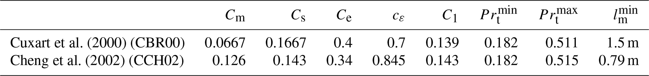
The ϕz function is bounded not to exceed as done in the Arpege model of Meteo France (e.g., Bazile et al., 2012). Assuming that the minimum of ϕz is attained in the linearly stratified limit (i.e., for ), values of the maximum Prandtl number are given in Table 1. Constant values for Cm, Cs, Ce, cε, and C1 can be determined from different methods, leading to nearly similar values. The traditional way is to use the inertial–convective subrange theory of locally isotropic turbulence (Lilly, 1967; Deardorff, 1974). Another way relies on a theoretical turbulence model partly based on renormalization group methods (see Cheng et al., 2002). For the present study, the sets proposed by Cuxart et al. (2000) and Cheng et al. (2002) will be considered (Table 1). A major difference between the two sets concerns the value of Cm. This difference is explained by a reevaluation of the energy redistribution among velocity components by pressure fluctuations, whose magnitude is assumed to be proportional to the degree of energy anisotropy as initially introduced by Rotta (1951). Note that the constant set of Cheng et al. (2002) is now used by default in both research and operational Meteo France models.
Cuxart et al. (2000)Cheng et al. (2002)Table 1Set of turbulence scheme constants from Cuxart et al. (2000) and Cheng et al. (2002). is the turbulent Prandtl number.
The Dirichlet boundary condition for TKE applied at the top z=ztop is m2 s−2 and at the bottom z=zsfc we have
with u⋆ and w⋆ the friction and convective velocities given by the bulk formulation. The value for emin has been chosen empirically as well as background values m2 s−1 and m2 s−1 for eddy diffusivities.
The minimum value for lm is simply set as . There are multiple options to compute the mixing lengths lm and lε (this point will be discussed later in Sect. 3.2.2), but all options have identical boundary conditions and
The value of Lsfc results from the similarity theory in the neutrally stratified surface layer (Sect. 4.1 in Redelsperger et al., 2001, and Appendix A). In Eq. (8), κ is the von Karman constant and z0 a roughness length computed within the bulk algorithm. The way esfc and Lsfc are obtained is detailed in Appendix A.
Our current implementation of boundary layer subgrid processes is an eddy-diffusivity approach which does not include any explicit representation of boundary-layer convective structures. This could be done via a mass-flux representation (e.g., Hourdin et al., 2002; Soares et al., 2004) or the introduction of a countergradient term (e.g., Troen and Mahrt, 1986). This point is left for future developments of the ABL1d model.
2.4 Processing of large-scale forcing and Newtonian relaxation
As mentioned earlier, the ABL1d model (1) requires three-dimensional large-scale atmospheric variables , while existing uncoupled oceanic forcing strategies require only two-dimensional (x,y) atmospheric variables. This is a difficulty for efficiency reasons since it substantially increases the number of I/Os but also for practical reasons because it requires the development of a dedicated tool to extract large-scale atmospheric data and interpolate them on prescribed geopotential heights from their native vertical grid, which can be either pressure based or arbitrary Lagrangian Eulerian. Such tools have been developed specifically to work with ERA-Interim, ERA5, and operational IFS datasets and are described in Appendix B.
Beyond the particular values of , the form of the relaxation timescale has a great impact on model solutions. The vertical profile for the λm and λs coefficients in Eq. (1) is chosen to nudge strongly above the MABL and moderately in the MABL with a smooth transition between its minimum and maximum value to avoid large vertical gradients in λm and λs, which would result in artificially large vertical gradients in atmospheric variables. In practice the λm(z) and λs(z) functions depend on the following parameters:
-
and , which define the maximum and minimum of the nudging coefficient for momentum and scalars respectively. Following Eq. (2), a guideline to set reasonable values for those parameter values would be to make sure that (i.e., the large-scale value is imposed above the boundary layer) and choose based on the typical adjustment timescale of the ABL to surface perturbations. Broadly speaking the ABL can be defined as the region that responds to surface forcings with a timescale of about an hour (e.g., LeMone et al., 2019). In the realistic numerical experiments shown in Sect. 5, we used , which, for an oceanic dynamical time step Δt=1080 s, would lead to . (i.e., the boundary layer values are the result of a weighting with a weight 0.8 for the ABL1d prediction and 0.2 for the large-scale value).
-
, which defines the extent of the transition zone separating the maximum and minimum of the nudging coefficient
We considered the following general form for λs(z) and λm(z), with hbl the boundary layer height whose value is diagnosed using an integral Richardson number criteria (Sect. 3.2 and 3.3 in Lemarié et al., 2012) with a critical value equal to C1:
where four αm coefficients are necessary to guarantee the continuity of λs(z) and its derivative ∂zλs at and . We easily find
The value of hbl is bounded beforehand to guarantee that at least 3 grid points are such that and . A typical profile of the λs(z) is shown in Fig. 1a.
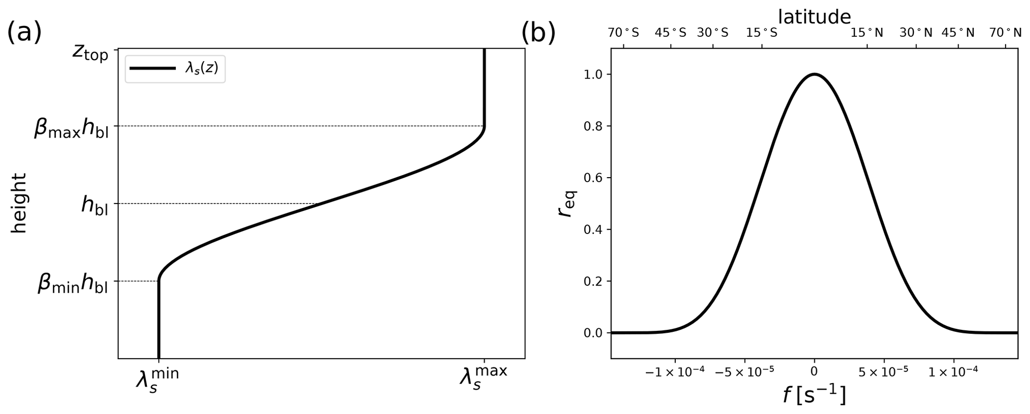
Figure 1(a) Typical profile of the nudging coefficient λs(z) with respect to the parameters . (b) Equatorial restoring function req with respect to the Coriolis frequency f.
When the model is forced by the large-scale pressure gradient (or the geostrophic winds), the parameter λm(z) should be theoretically zero at high and middle latitudes. However, for the equatorial region, a Newtonian relaxation toward the large-scale winds should be maintained. To do so, the coefficient λm(z) is multiplied by a coefficient req, which is a function of the Coriolis parameter f. The req coefficient is equal to zero for large values of and increases to 1 when approaching the Equator. The following form satisfies those constraints (see also Fig. 1b):
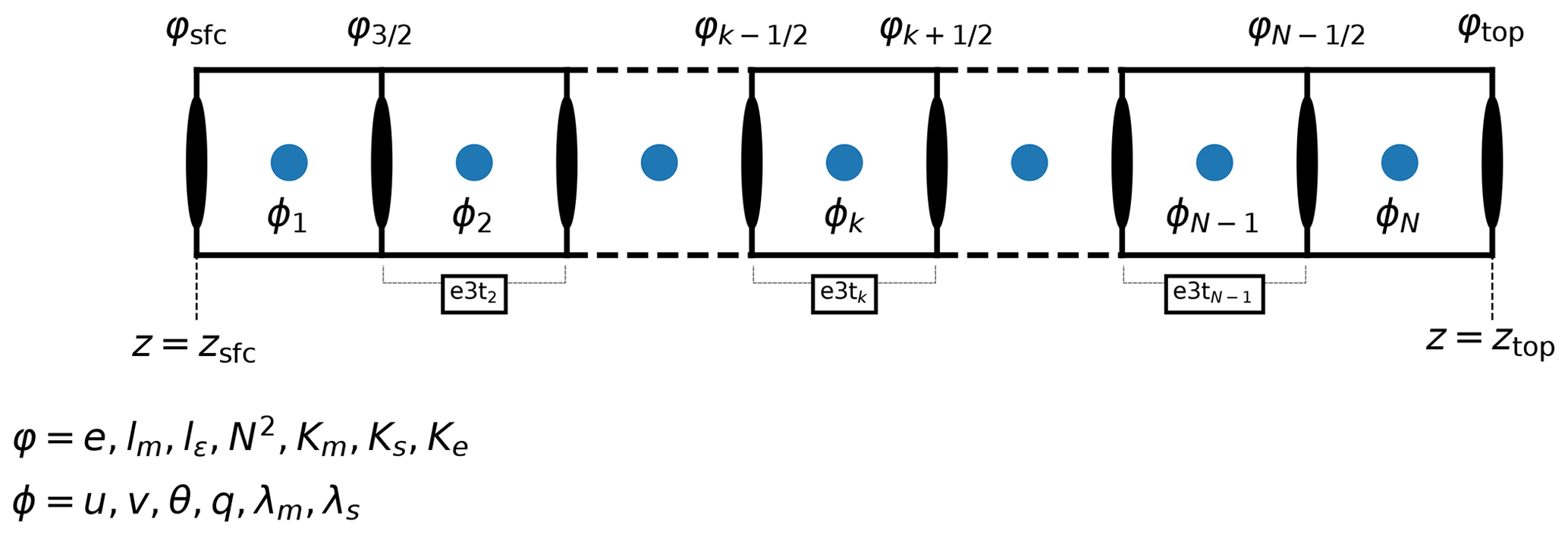
We have introduced so far the continuous formulation of the ABL1d model. In this section we describe the discretization methods used and how this model is included in the NEMO modeling framework. In particular, the discretization of the Coriolis term and of the TKE Eq. (6) and associated mixing lengths are described in Sect. 3.1 and 3.2 respectively. Details about the practical implementation in NEMO are given in Sect. 3.3 for the coupling aspects and 3.4 for the computational aspects. The ABL1d model (1) is discretized in time with an Euler backward scheme for the vertical diffusion terms, semi-implicitly for the Coriolis term, and explicitly for the relaxation term, which means that the model is stable as long as λsΔt≤1. The variables are defined on a non-staggered grid in the horizontal (a.k.a Arakawa A-grid). Because we consider a computational domain exclusively over water or sea ice, topography is not considered and vertical levels are flat and fixed in time which, among other things, allows the large-scale data ϕLS to be interpolated on the vertical grid offline. The position of the various quantities introduced so far on the computational grid is given in Fig. 2.
3.1 Coriolis term treatment
Since in our implementation the horizontal velocity components are collocated, the discretization of the Coriolis term is straightforward and is energetically neutral. In the event the ABL1d is integrated with a time step much larger than the oceanic time step, specific care must be given to the stability of the Coriolis term time stepping. A semi-implicit scheme with weighting parameter γ reads , where the exponent ⋆ is used here to emphasize that is a temporary value at time n+1 before vertical diffusion and Newtonian relaxation are applied. For a given grid cell with index (i,j), the semi-implicit scheme can be written in a more compact way as
The associated amplification factor modulus is meaning that unconditional stability is obtained as long as . For the numerical results obtained below in Sects. 4 and 5 we used γ=0.55, which is deliberately slightly dissipative.
3.2 Discretization of TKE equation
In Sect. 2.3 we have presented the continuous formulation of the TKE-based turbulence closure of the ABL1d model. In the following we describe how the positivity of TKE can be preserved and how the mixing lengths lm and lε are computed. We provide a substantial discussion on the latter aspect because numerical results are very sensitive to the choices made.
3.2.1 TKE positivity preservation
The TKE equation is discretized using a backward Euler scheme in time with a linearization of the dissipation term , which is discretized as . However, such discretization is not unconditionally positivity-preserving for TKE, which could give rise to unphysical solutions (e.g., Burchard, 2002b). Ignoring the diffusion term, the TKE prognostic Eq. (6) can be written as an ordinary differential equation (ODE) of the form
where the last term can be seen as a damping term. For ODEs like Eq. (11) it can be shown that for an initial condition e(0)≥0 and , the solution e(t) keeps the same sign as e(0) whatever the sign of the damping coefficient D(e,t). Assuming that S(uh,N2) and D(e,t) are positive, a backward Euler discretization of the damping term in Eq. (11) would lead to , which preserves positivity since for en≥0 we obtain . However, there is no guarantee that the forcing term S(uh,N2) is positive, in particular when the shear is weak and the stratification is large. When S(uh,N2) is negative a specific treatment (known as the “Patankar trick”; see Deleersnijder et al., 1997; Burchard, 2002b) is required. In the event of a negative S(uh,N2), the idea is to move the buoyancy term from S to D after dividing it by en, such that is now strictly positive and . Such a procedure is a sufficient condition to preserve the positivity of the TKE without ad hoc clipping of negative values. Moreover our discretization of the shear and buoyancy terms in the TKE equation is done in an energetically consistent way following Burchard (2002a).
3.2.2 Mixing length computation
Another challenging task when implementing a TKE scheme is the discretization of the mixing lengths. As mentioned earlier, four different discretizations of lm (lε) have been coded. All discretizations consider the boundary conditions given in Eq. (8). The values of lm and lε are traditionally computed from two intermediate length scales lup and ldwn, which respectively correspond to the maximum upward and downward displacement of a parcel of air with a given initial kinetic energy. Once lup and ldwn have been estimated by one of the methods described below, the dissipative and mixing length scales lm and lε are computed as
where for CBR00 and for CCH02 (see Appendix A). The impact of the weighting between lup and ldwn to compute lm can be significant for idealized experiments like the ones presented in Sect. 4.2 but for more realistic cases results are weakly sensitive and equivalent to the ones obtained with the simpler weighting .
In the following we provide the continuous form of the various ways to compute lup and ldwn implemented in the ABL1d model. The discretization aspects are detailed in Appendix C.
-
Bougeault and Lacarrère (1989) length scale. A classical approach in atmospheric models is the use of the Bougeault and Lacarrère (1989) mixing length (see also Bougeault and André, 1986) which defines lup and ldwn as
By construction such mixing lengths are bounded by the distance to the bottom and the top of the computational domain. It is worth noting that for constant values of N2, Eq. (13) gives and respectively, which is equivalent to the Deardorff (1980) length scale. In the remainder we will note lBL89, the mixing length obtained from Eq. (13).
-
Adaptation of NEMO's length scale. The standard NEMO algorithm (Sect. 10.1.3 in Madec, 2012) is simple and efficient compared to Eq. (13). This algorithm is based on the Deardorff (1980) length scale . lup and ldwn are first initialized to . The resulting length scales are then limited not only by the distance to the surface and to the top but also by the distance to a strongly stratified portion of the air column. This limitation amounts to control of the vertical gradients of lup(z) and ldwn(z) such that they are not larger than the variations of altitude. The resulting mixing length will be simply referred to as lD80. Note that the Taylor expansion of the integral in Eq. (13) is
which shows that the lD80 mixing length is an approximation of lBL89, which is obtained by retaining only the leading order term in the Taylor expansion.
-
Rodier et al. (2017) length scale. Recently, Rodier et al. (2017) proposed a modification of the Bougeault and Lacarrère (1989) mixing length. This modification turns out to improve results for stably stratified boundary layers typical of areas covered by ice. They propose to add a shear-related term to Eq. (13) such that the definition of lup and ldwn becomes
where c0 is a parameter whose value should be smaller than . The value of c0 will be chosen based on numerical experiments presented in Sect. 4. In the following this mixing length will be referred to as lR17.
-
A local buoyancy- and shear-based length scale. For the sake of computational efficiency, we have derived a local version of the Rodier et al. (2017) length scale which is original to the present paper. Under the assumption that lup (ldwn) is small compared to the spatial variations of N2, e, and , we end up with the following second-order equation for lup:
whose unique positive solution is
We easily find that for , and for N2=0, which is consistent with the shear-based length scale of Wilson and Venayagamoorthy (2015). Once has been computed we apply the same algorithmic approach as in the lD80 case.
The performance of those four length scales for various physical flows is discussed in Sect. 4.
3.3 Coupling with ocean and sea ice
For the practical implementation of the ABL coupling strategy within a global oceanic model, a proper coupling method is required for stability and consistency purposes (e.g., Beljaars et al., 2017; Renault et al., 2019a), and the ABL1d must have the ability to handle grid cells partially covered by sea ice. For the coupling strategy, a so-called implicit flux coupling which is unconditionally stable (Appendix B in Beljaars et al., 2017) and asymptotically consistent for Δt→0 (Renault et al., 2019a) is used. Because vertical diffusion in ABL1d is handled implicitly in time, the boundary conditions (Eqs. 3 and 4) should be provided at time n+1. The implicit flux coupling amounts to discretize the boundary conditions Eqs. (3) and (4) as
where and are either the instantaneous values at time n if NEMO and ABL1d have the same time step or an average over the successive oceanic substeps otherwise.
Particular care has also been given to the compatibility between the ABL1d model and SI3 (Sea Ice model Integrated Initiative) the sea-ice component of NEMO. SI3 is a multi-category model whose state variables relevant for our study are the ice surface temperature with associated fractional area al (for the lth category), and the ice velocity uice (same for all categories). Note that the values of the exchange coefficients over sea ice , , and are different from their oceanic counterparts but are the same over all sea-ice categories. At this point there are several strategies for the ABL1d∕SI3 coupling:
-
Run the ABL1d model over the whole ABL for each category l and then average atmospheric variables weighted by al.
-
Run a single ABL1d model with a category-averaged surface flux. In the current version of NEMO is a function of the averaged temperature Tice which means that it is equivalent to compute a flux over each category before averaging them and to compute a single flux using the averaged surface temperature, indeed
The second option has been preferred because it is much easier to implement and more computationally efficient. It amounts to consider an ice surface temperature averaged over all categories for the computation of ice–atmosphere turbulent fluxes (Tice also enters in the computation of qice). Noting Foce the fraction of open water (lead), the boundary condition (15) and (16) are modified in
Because the dynamics of sea ice is computed before the thermodynamics (see Fig. 1 in Rousset et al., 2015), the ABL1d–SI3 coupling follows these different steps:
-
compute surface fluxes over ice and ocean and integrate the ABL1d model for given values and ,
-
compute the dynamics of sea ice,
-
update and in and because of step 2,
-
distribute the fluxes over each ice category considering the updated values (Sect. 3.6 in Rousset et al., 2015)
-
compute the thermo-dynamics of sea ice.
3.4 Computational aspects
As described in Maisonnave and Masson (2015), the NEMO source code is organized to separate the ocean routines on one side and the routines responsible for the surface boundary conditions computation (including sea ice and the coupling interfaces) on the other side. This makes a clear separation between the standard ocean model (OCE component) and the so-called surface module (SAS component). As schematically described in Fig. 3, the ABL1d model has been implemented within the SAS component, which allows the following useful features:
-
The ABL1d model can be run in standalone mode (coupled or not with sea ice) with prescribed oceanic surface fields.
-
The ABL1d model can be run in detached mode; i.e., the OCE and SAS components run on potentially separate processors and computational grids communicating via the OASIS3-MCT coupling library (Craig et al., 2017).

Figure 3Schematic representation of the ASL forcing strategy (left) and ABL coupling strategy (right) in terms of code organization and required external data. The OCE and SI3 components represent the oceanic and sea-ice dynamics and thermodynamics respectively while the ASL component is in charge of providing boundary conditions related to atmospheric conditions. In the NEMO computational framework the so-called surface module (SAS component), delineated by dashed line polygons, is virtually separated from the OCE component, which allows SAS to be run in standalone or detached mode (see Sect. 3.4).
An other capability implemented within the NEMO modeling framework is the possibility to interpolate forcing fields on the fly. This is particularly useful for the ABL coupling strategy since three-dimensional atmospheric data must be interpolated on the ABL1d computational grid. As the current implementation of the on-the-fly interpolation only works in the horizontal, the vertical interpolation of large-scale atmospheric data on the ABL1d vertical grid is done offline. Nevertheless it means that the size of input data compared to an ASL forcing strategy is N times larger with N the number of vertical levels in the ABL. A possibility to improve the efficiency for the reading of input data would be to take advantage of the parallel I/O capabilities provided by the XIOS library (XML-IO-Server; Meurdesoif et al., 2016) which is currently used in NEMO only for writing output data. This technical development is left for future work. This is a key aspect because, as discussed later in Appendix D, the main source of computational overhead associated with the ABL coupling strategy is due to the time spent waiting for input files to be read.
Table 2Description of the idealized experiments performed in Sect. 4. LMO is the Monin–Obukhov length.

4.1 Sensitivity experiments and objectives
To check the relevance of our ABL1d model for idealized atmospheric situations typical of the atmospheric boundary layer over water or sea ice, we performed a set of single-column experiments. Each of those experiments are evaluated with benchmark large eddy simulations (LESs). Moreover, we use standardized test cases from the literature to allow our results to be cross-compared with other well-established ABL schemes. In the following we consider a neutrally stratified (Sect. 4.2) and a stably stratified (Sect. 4.3) case as well as a case with a transition from stable to unstable stratification representative of an atmospheric flow over an SST front (Sect. 4.4). All ABL1d simulations presented here have been performed directly within the SAS component of the NEMO modeling framework and can be reproduced using the code available at https://zenodo.org/record/3904518 (last access: 20 January 2021) (Lemarié and Samson, 2020), which also includes the scripts to generate the figures. An objective of the present section is to illustrate the type of sensitivity we can expect from the ABL1d model and discriminate between the various options available in the code. The experiments showed in Sect. 4.2 and 4.3 are meant to investigate the impact of (i) the set of constant coefficients (CBR00 vs. CCH02), (ii) the various formulations of lm and lε among the algorithms described in Sect. 3.2.2, and (iii) the parameter value c0 in the lR17 and mixing length computation. Those experiments will allow several options to be discarded. The ability of the remaining options to represent the downward mixing mechanism, discussed in Sect. 1.2, is then evaluated in Sect. 4.4. The robustness of the results to the bulk formulation and to the nudging coefficient is also checked. For each experiment we explicitly provide the initial and boundary conditions as well as all the necessary parameter values (see Table 2) so that the experiments can be reproduced easily by other modeling groups.
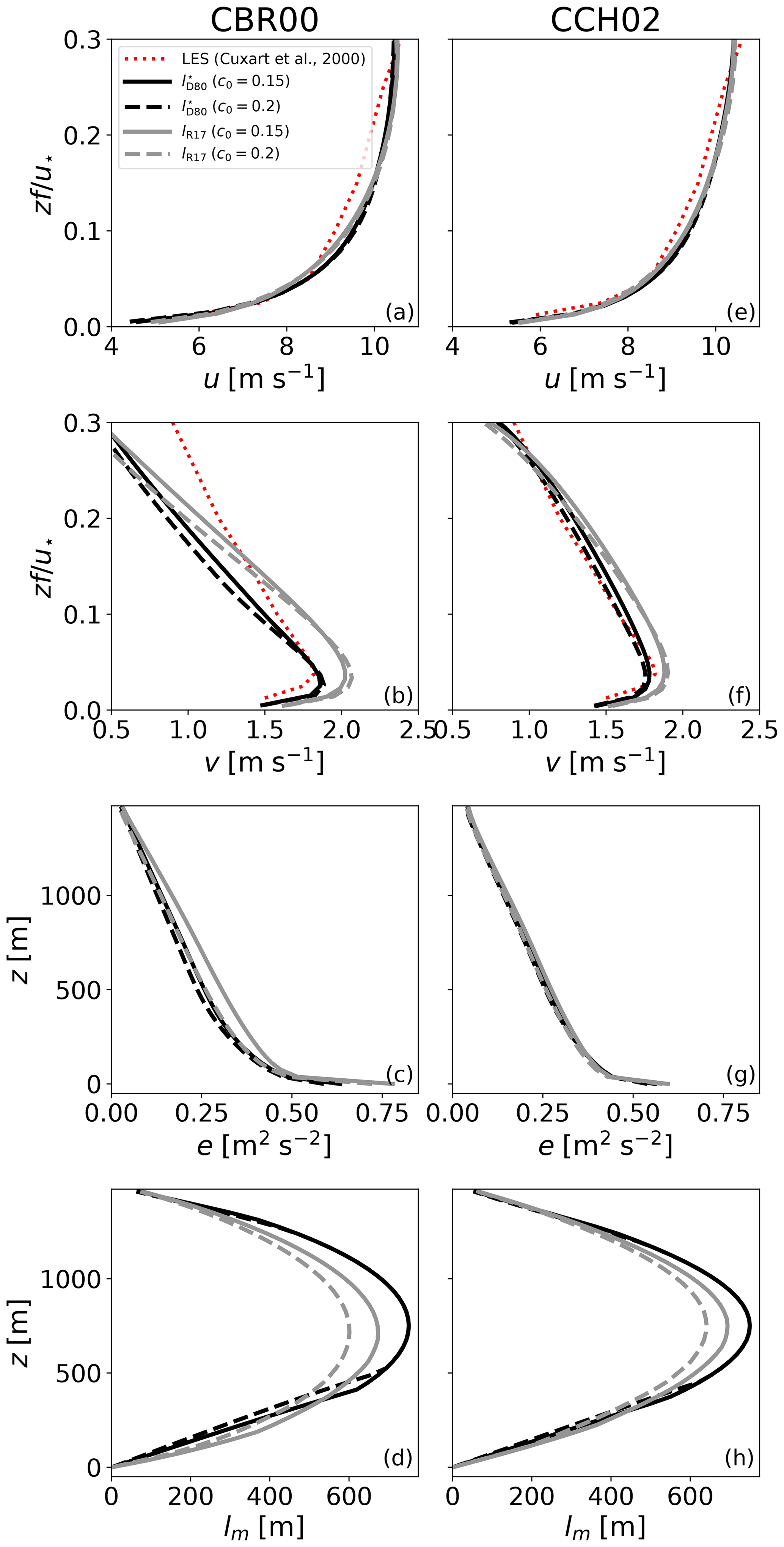
Figure 4Results obtained for the neutral boundary-layer case of Andren et al. (1994) with the CBR00 model constants (left panels, a to d) and CCH02 model constants (right panels, d to e) for different parameter values for c0 and different mixing-length formulations ( for black lines or lR17 for gray lines). Results are shown for u (a, e), v (b, f), e (c, g), and lm (d, h). In the top four panels results are compared with LESs from Cuxart et al. (2000) (their Fig. 16). As in Andren et al. (1994), simulations were run over a period of 10∕f and results are averaged over the last 3∕f period.
4.2 Neutral turbulent Ekman layer
We first propose to investigate the simulation of a neutrally stratified atmosphere analogous to a classical turbulent Ekman layer. The selected case is based on the setup described in Andren et al. (1994). The initial conditions for this experiment are not defined analytically; they are given by Table A1 in Andren et al. (1994)2. This test case is mainly used to check the adequacy of our surface boundary conditions with similarity theory and the proper calibration of the parameter c0 in the and lR17 formulations of the mixing lengths. In theory, the lD80 and lBL89 mixing lengths do not support the asymptotic limit N2=0 but for the integrity of numerical results a minimum threshold on the stratification is imposed in the code. In this case the procedure to compute those mixing lengths as described in Appendix C will provide identical results, namely and (i.e., the distance from the top and from the bottom of the computational domain). We test here the and lR17 introduced in Sect. 3.2.2. The reference solution is taken from Cuxart et al. (2000) (panels a and b in their Fig. 16). Results are obtained using the ABL1d model with either the CBR00 (Fig. 4a–d) or the CCH02 (Fig. 4e–h) set of parameters. All experiments have been done with c0=0.15 and c0=0.2. All simulations are able to reproduce the overall behavior of the LES case. The main outcomes are as follows:
-
The best agreement is obtained when using the CCH02 constants along with mixing length and c0=0.2.
-
The results obtained for lD80 and lBL89 are identical and close to the lR17 results with c0=0.15 (not shown).
-
All simulations with the CCH02 set of parameters show reasonable results.
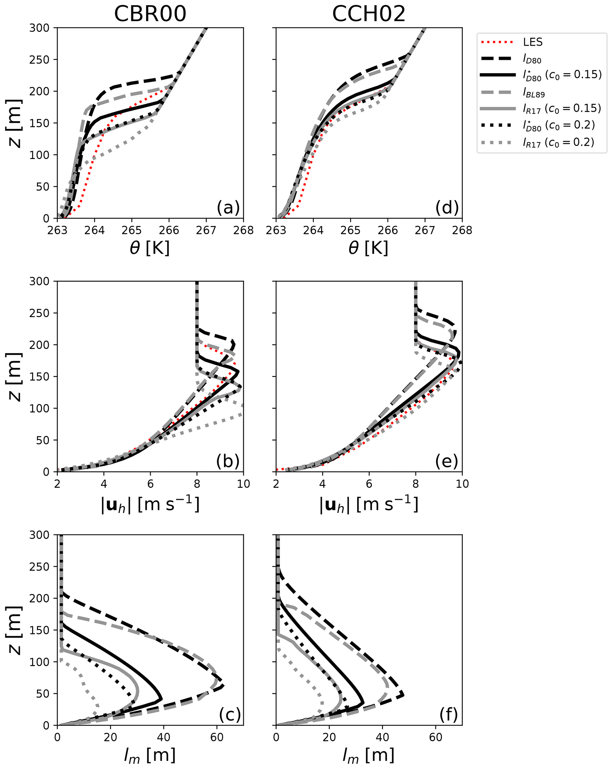
Figure 5Results obtained for the stably stratified boundary-layer case of Cuxart et al. (2006) for the parameter values CBR00 (left panels, a to c) and CCH02 (right panels, d to f) with different mixing-length formulations: lD80 for black solid lines, with c0=0.15 for dashed black lines (c0=0.2 for dotted black lines), lBL89 for solid gray lines, and lR17 with c0=0.15 for dashed gray lines (c0=0.2 for dotted gray lines). Results are shown for potential temperature θ (a, d), wind speed (b, e), and lm (c, f). Dotted red lines represent LES results from Rodier et al. (2017). Instantaneous profiles after 9 h are shown.
4.3 Stably stratified boundary layer (GABLS1)
Within the Global Energy and Water Exchanges (GEWEX) atmospheric boundary layer study (GABLS), idealized cases for stable surface boundary layers have been investigated (e.g., Cuxart et al., 2006). Such conditions are typical of areas covered with sea ice. Here we consider the GABLS1 case, whose technical description is available at http://turbulencia.uib.es/gabls/gabls1d_desc.pdf (last access: 20 January 2021). This experiment is particularly interesting as significant differences generally exist between solutions obtained from LES and single-column simulations, for example when the Bougeault and Lacarrère (1989) length scale is used (e.g., Cuxart et al., 2006; Rodier et al., 2017). A large-scale geostrophic wind is imposed as well as a cooling of the surface temperature θs(t) given by . The parameter values for this test are reported in Table 2 and the initial conditions are , and
The solutions after 9 h of simulation are shown in Fig. 5 (left panels) for CBR00 parameter values and in Fig. 5 (right panels) for CCH02 parameter values. The reference solution is taken from Rodier et al. (2017) LESs. As expected, solutions based on a mixing length ignoring the contribution from the vertical shear exhibit a boundary layer that is too thick and a wind speed maximum located too high in altitude. Using a buoyancy- and shear-based mixing length mitigates the issue and provides very good agreement with reference solutions when the CCH02 model constants are used. The best results are obtained for with c0=0.2 and lR17 with c0=0.15. Solutions obtained with the CBR00 model constants systematically predict larger turbulent kinetic energy and mixing lengths, resulting in large values of Ks in the first 100 m near the surface (not shown). The mismatch in terms of TKE is partially explained by the difference in boundary conditions since with CBR00 constants we have while with CCH02 constants we get from Eq. (7). Note that the proper calibration of the c0 constant jointly with the cε is the subject of several ongoing studies. Since our simulations reproduce the known sensitivity to those parameters, the ABL1d model could directly benefit from new findings on that topic.
The main outcomes are as follows:
-
The CCH02 set of parameters provides results of better quality than the CBR00 constants. For the sake of simplicity, we will retain only the CCH02 parameters for the numerical results shown in the remainder.
-
The buoyancy- and vertical-shear-based mixing lengths lR17 and are superior to the buoyancy-based mixing lengths lD80 and lBL89 for stable boundary layers.
4.4 Winds across a midlatitude SST front
4.4.1 Setup and reference solutions
An idealized experiment particularly relevant for the coupling of the MABL with mesoscale oceanic eddies (and potentially submesoscale fronts) was initially suggested by Spall (2007) and then revised by Kilpatrick et al. (2014). More recently Ayet and Redelsperger (2019) derived an analytical model based on a similar setup. The geometry of the problem is two-dimensional x–z with an SST front along the x axis:
where Δθ=3 K, Lθ=100 km, and . As indicated in Table 2, a zonal geostrophic wind of 15 m s−1 is prescribed, balanced by a vertically homogeneous meridional pressure gradient. The wind thus flows over cold water before reaching a warm SST anomaly, which is 3 K warmer. We consider a dry case, in which the model is initialized ∀x with
where s−2 and θref=288 K.
The velocities are systematically initialized with geostrophic winds. All simulations are run for 36 h when the flow reaches a quasi-equilibrium state. For this configuration the reference solution is obtained from the mesoscale non-hydrostatic model (MesoNH) v5.3.0 (Lafore et al., 1998; Lac et al., 2018), where microphysics and radiation packages have not been activated. The horizontal resolution is Δx=1 km and the model is discretized with 91 vertical levels from the surface to 20 km height. The vertical resolution near the surface is Δz=10 m and around Δz=100 m at 2000 m height. The turbulence scheme is the 1.5-order closure of Cuxart et al. (2000) in its one-dimensional form with the lBL89 mixing length and CCH02 set of parameters. Sea surface fluxes are computed using the bulk parameterization COARE3.0, which is also available in NEMO from the AeroBulk package. As far as the ABL1d model is concerned, the top of the computational domain is ztop=2000 m and the vertical grid is stretched with a typical resolution of 20 m near the surface and 100 m near z=ztop with a first grid point located at z=10 m. In the horizontal, the resolution is Δx=6 km.
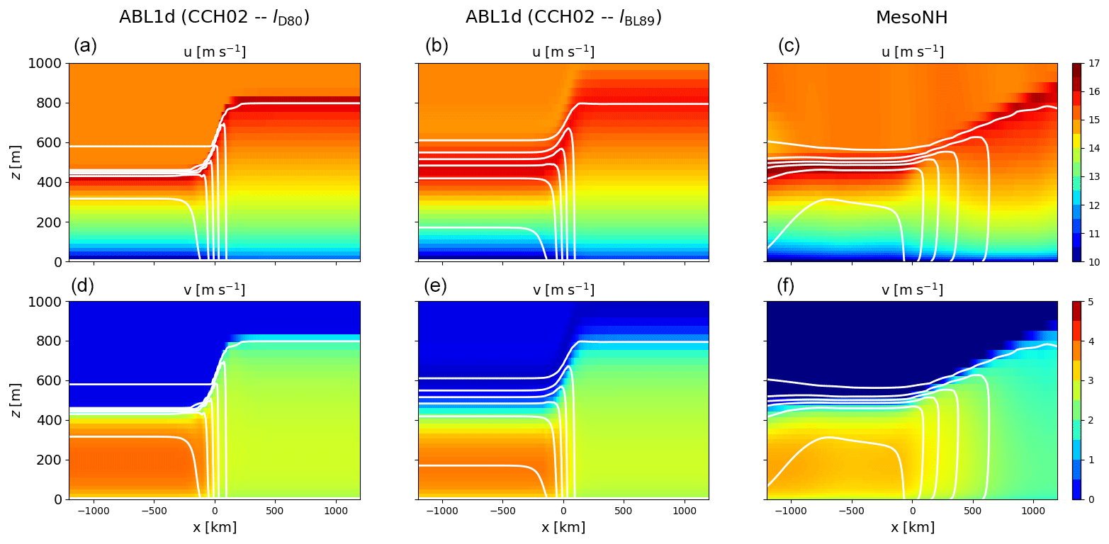
Figure 6Zonal (a, b, c) and meridional (d, e, f) components of atmospheric winds for the reference MesoNH simulation (c, f), for ABL1d simulations with lD80 mixing length and CCH02 model constants (a, d), and with lBL89 mixing length and CCH02 model constants (b, e). Temperature contours are shown in white with a contour every 0.5 ∘C between 15 and 17.5 ∘C. The SST front is centered at x=0 km.

Figure 7Zonal (a) and meridional (b) components of 10 m winds and 10 m temperature (c) for the reference MesoNH simulation (dashed red) and for ABL1d simulations with different mixing-length formulations for the winds across a midlatitude SST front experiment.
4.4.2 Numerical results
For this configuration, results will be mostly evaluated in terms of 10 m winds u10 and temperature θ10. As an illustration of the type of result we get, we first compare the MesoNH solution and the ABL1d solution obtained with the lD80 and lBL89 mixing lengths in Fig. 6. It is worth noting that the MesoNH solution closely compares with the solution of Kilpatrick et al. (2014) (their Fig. 2) with a shallow boundary layer height (around 400 m) before the front and a thicker one (around 800 m) after the front where momentum mixing is enhanced. Over the front, as noted by Ayet and Redelsperger (2019) with a similar setup, the effect of advection is predominant for meridional winds, thus explaining the differences seen with the ABL1d simulations. Indeed with ABL1d, whatever the numerical options, the atmospheric column will locally adjust to the underlying oceanic conditions since horizontal advection is neglected. This explains the absence of horizontal lag when passing over the front in the ABL1d solution compared to the MesoNH solution. However, away from the SST front the solutions are very similar in terms of boundary layer height and vertical wind structure. In anticipation of a coupling with an oceanic model, the most important quantities to look at are the 10 m atmospheric variables rather than the full 3D vertical structure of the MABL. In Fig. 7, the 10 m wind components and temperature when the ABL1d model reaches a quasi-equilibrium state are shown for different mixing length options, as well as the MesoNH results. First, the results obtained with the lR17 are very different from the expected behavior, and we will focus the discussion on other options. In terms of zonal 10 m wind the buoyancy-based lBL89 and lD80 mixing lengths provide a good agreement with the MesoNH solution, which could be expected as the MesoNH solution has been generated using the lBL89 mixing length. As soon as the mixing length is a function of buoyancy and vertical shear (as is the case for ) the simulated winds are weaker because the boundary layer is thinner. This leads to improved results in the stably stratified case shown earlier, but in the present case, which is more representative of realistic configuration in the MABL, it leads to a mixing that is too weak. However, compared to the lR17 mixing length the still performs reasonably well but the winds on the warm side of the front are about 1 m s−1 weaker than the MesoNH winds for c0=0.15 and become weaker and weaker as c0 increases.
The main outcomes are as follows:
-
In the frontal region the effect of horizontal advection is predominant and the ABL1d model cannot reproduce the horizontal lag seen in the reference solution when passing over the front.
-
The ABL1d model reproduces the downward momentum mixing mechanism correctly. The best results are obtained with the buoyancy-based lBL89 and lD80 mixing lengths.
-
The lR17 mixing length will be discarded from the comparison.
Although relevant for the present study this 2D x–z setup is not fully representative of realistic conditions because the air column has time to adjust to the underlying oceanic state, which is kept frozen in time.
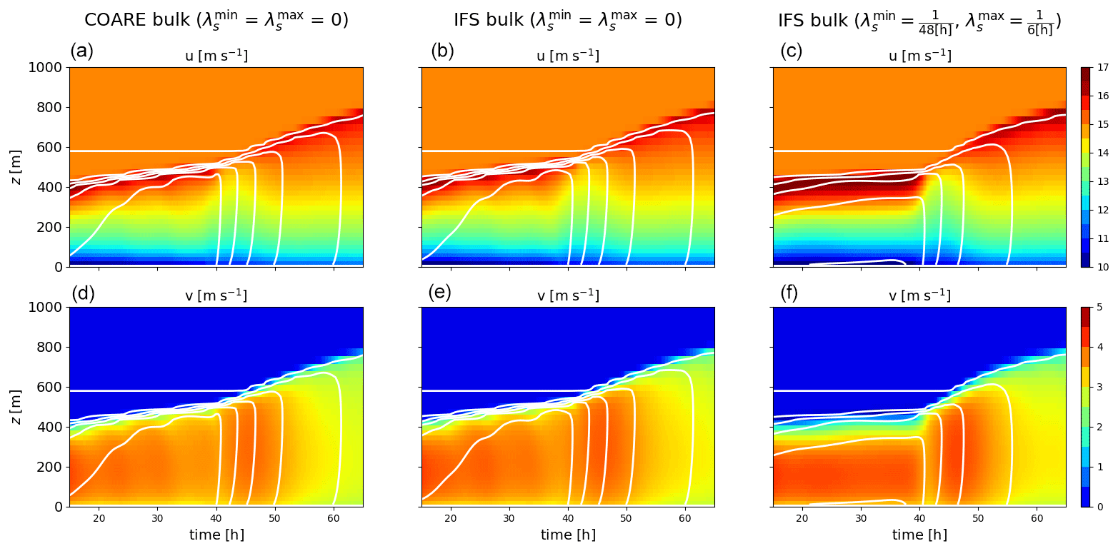
Figure 82D time vs. height sections representing the temporal evolution of the zonal (a, b, c) and meridional (d, e, f) components of atmospheric winds for ABL1d simulations of an air column crossing an SST front with COARE bulk formulation (a, d) and IFS bulk formulation (middle and right panels). For the case presented in the right panels, a Newtonian relaxation toward the initial temperature profile was added with and . The simulations were performed with lD80 mixing length and CCH02 model constants.
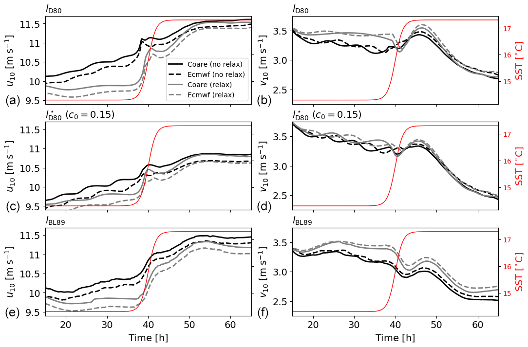
Figure 9Temporal evolution of the zonal (a, c, e) and meridional (b, d, f) components of 10 m atmospheric winds for ABL1d simulations of an air column crossing an SST front. The temporal evolution of SST (solid red lines) is also shown. For each panel the results from four different simulations are shown: with COARE bulk formulation (solid lines) or IFS bulk formulation (dashed lines), with Newtonian relaxation on temperature such that and (gray lines) or no relaxation (black lines). Panels (a, b) are obtained from simulations performed with lD80 mixing length, (c, d) with (c0=0.15), and (e, f) lBL89.
4.4.3 A single-column version
An alternative to the x–z setup would be to formulate the test case as a Lagrangian advection of an air column over an SST front by prescribing a temporal evolution of sea surface temperature θs(t) as
In this case the air column does not necessarily have time to adjust to the underlying oceanic conditions. Initial conditions are the same as the ones of the 2D x–z case. For this test case we do not have a reference solution, but it is expected that the temporal evolution of the solution should be relatively similar to the spatial evolution in the MesoNH 2D x–z case studied in previous subsection. This can be seen from Fig. 8, where there is a clear similarity between the time vs. height sections obtained with the ABL1d simulations and the x vs. height sections shown for MesoNH in Fig. 6. The ABL1d solution shows a temporal lag analogous to the horizontal lag in the reference solution for the 2D x–z case. In addition to that, we also use this test case to investigate the sensitivity of the solutions to the bulk formulation and to the Newtonian relaxation which was absent in simulations discussed so far. We consider the COARE and IFS bulk formulations, which are relatively close to each other, to check the robustness of the results to small perturbations in surface fluxes. We also consider simulations with a relaxation of the temperature variable toward the initial condition with a fast relaxation timescale above the ABL and a slower one in the ABL. This is meant to check that the relaxation does not completely overwrite the physics of the coupling we aim to represent with the ABL1d model. Results from those sensitivity experiments are shown in Figs. 8 and 9. In particular in Fig. 9 the evolution of the 10 m winds across the SST front closely resembles the one shown in Fig. 7 (dashed red lines) for MesoNH. Moreover, the results in Fig. 9 are robust to a change of bulk formulation to compute the surface fluxes. Reassuringly, adding a relaxation toward large-scale data which did not see the SST front does not deteriorate the realism of the solutions, as can be seen from Fig. 8c and f and 9 (gray lines).
The main outcomes are as follows:
-
The response of the ABL1d model to evolving oceanic conditions is not local in time (it shows a temporal lag).
-
The good representation of the downward momentum mixing process is not sensitive to the bulk formulation.
-
Adding a relaxation term toward large-scale data does not deteriorate the realism of the solutions significantly.
Based on the results reported in this section, the best balance between efficiency and physical relevance is obtained when using the parameter values from CCH02 and the modified Deardorff (1980) mixing-length formulation lD80 or . In particular we could imagine using the lD80 formulation over water and the formulation over sea ice.
Using atmosphere-only experiments, we have been focused so far on the good representation of the downward momentum mixing mechanism and of the stable boundary layers typical of areas covered with sea ice. In the following we check that those two aspects are still adequately represented in a realistic coupled NEMO-ABL1d simulation. This simulation will also be used to look at the wind–current interaction, which was left aside so far. We performed a 5-year global simulation using the ORCA025 configuration. Details and illustrations are given hereafter.
5.1 Coupled NEMO-ABL1d configuration
We use here a global ORCA025 configuration at a 0.25∘ horizontal resolution (Barnier et al., 2006) with 75 vertical z levels forced by the ECWMF ERA-Interim 6 h analysis (Dee et al., 2011). This configuration is identical to the one described in Couvelard et al. (2020) (see their Sect. 4.1.1). The ABL1d-NEMO coupled simulation is carried out with the same numerical options as in a standard ASL forcing strategy. However, in the ABL coupling strategy, the two-dimensional near-surface air temperature, humidity, and winds used in the usual ASL forcing are replaced by three-dimensional atmospheric variables sampled between the surface and 2000 m preprocessed following the different steps described in Appendix B. The large-scale pressure gradient computed during the preprocessing is used as a geostrophic forcing for the ABL1d model dynamics. Three-dimensional atmospheric variables are generated over the 2014–2018 period and vertically interpolated on 50 levels between 10 and 2000 m with a vertical resolution increasing with height. Grid resolution is about 20 m near the air–sea interface and reaches 70 m at the top of the ABL1d domain. The choice of a vertical extent of 2000 m and 50 vertical levels in the ABL1d model is somewhat arbitrary and the robustness of numerical results to these choices will be investigated in future studies. For the simulations presented here, the same horizontal grid and time step (Δt=1200 s) are chosen in the ABL1d and NEMO models. The options associated with the ABL coupling available through the NEMO standard name list are reported in Table 3, and a detailed profiling of the code is presented in Appendix D in order to assess the overhead associated with the ABL coupling strategy vs. ASL coupling strategy. This profiling shows that the overhead associated with the ABL1d (when using the lD80 mixing length) is on the order of 4 % and the one associated with the input part of the I/O operations is 5 %. Overall there is an increase of 9 % in elapsed time compared to the standard ASL forcing strategy.
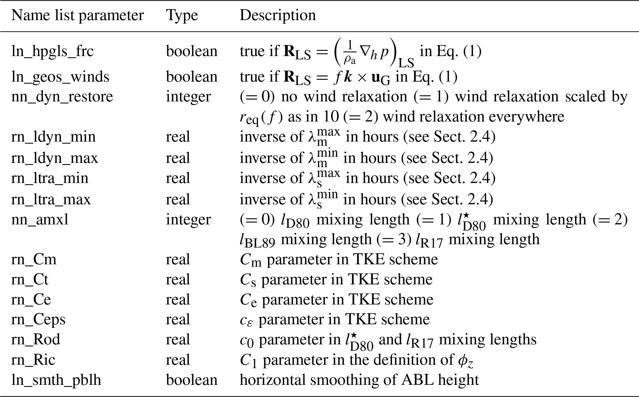
Table 3Name list parameters in the NEMO(v4.0) to set in the name list section namsbc_abl before running a simulation coupled with ABL1d.
5.2 Numerical results
In this section, we evaluate the ABL coupling strategy in a realistic context for a set of relevant metrics. The objective is not to conduct a thorough physical analysis of the numerical results but to illustrate the potential of the ABL coupling strategy and its proper implementation in NEMO. To evaluate our numerical results, we use standard metrics from the literature to quantify the wind–SST (a.k.a. thermal feedback effect), wind–currents (a.k.a. current feedback effect), and MABL–sea-ice couplings (e.g., Bryan et al., 2010; Renault et al., 2019b).
5.2.1 Thermal feedback effect
To quantify the surface wind response to SST, we show in Fig. 10a a global map of the temporal correlation between the high-pass-filtered 10 m wind speed from the first vertical level in the ABL1d model and the SST. The same correlation is shown in Bryan et al. (2010) from satellite observations (their Fig. 1d) and from coupled numerical experiments between a 0.1∘ ocean and a 0.25∘ atmospheric model (their Fig. 1c). Consistent with observations and fully coupled models, the correlation obtained from the coupled NEMO-ABL1d simulation shows large positive correlations over regions like the Southern Ocean, Kuroshio, and Gulf Stream extensions as well as in the Gulf of Guinea. Correlations are, however, weaker than observations in the northern and equatorial Pacific between 90 and 180∘ W. As the thermal feedback strength is related to the ocean model resolution (Bryan et al., 2010), we can expect a better agreement with observations using a higher resolution configuration such as ORCA12 ( resolution). This coupling sensitivity to the oceanic resolution will be addressed in a future study.
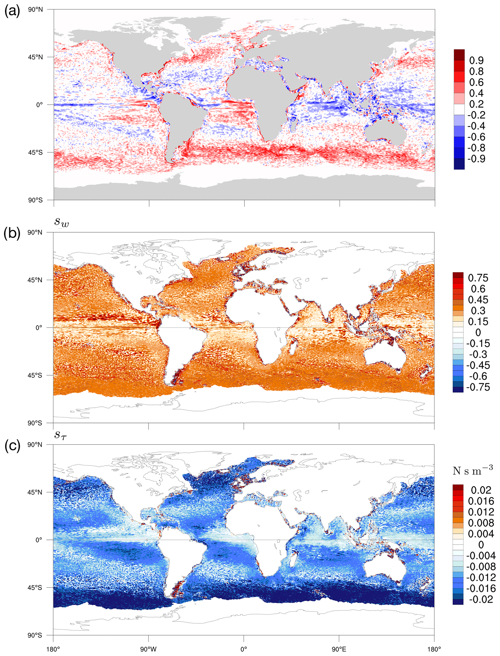
Figure 10(a) Global map of temporal correlation of high-pass-filtered wind speed at the first vertical level of the ABL1d model with SST from NEMO. Both NEMO and ABL1d are configured at 0.25∘ resolution. (b, c) Global maps of the coupling coefficient between the surface current vorticity and the wind curl (sw, b) and between the surface current vorticity and the wind-stress curl (sτ, c) estimated from a 0.25∘ resolution coupled NEMO-ABL1d global simulation. The fields are first temporally averaged using a 29 d running mean and spatially high-pass filtered.
5.2.2 Current feedback effect
Other processes of interest are those related to the coupling between oceanic surface currents, wind stress, and wind. Such coupling is responsible for a dampening of the eddy mesoscale activity in the ocean. In Renault et al. (2019b), two coupling coefficients called sw and sτ are defined to quantify this effect. sτ is a measure of the sink of energy from the eddies and fronts to the ABL and sw quantifies the partial re-energization of the ocean by the wind response to the wind–current coupling. This re-energization is absent in the ASL forcing strategy, which results in an excessive dampening of the oceanic eddy mesoscale activity. In practice, sτ (sw) corresponds to the slope of the linear relationship between high-pass-filtered surface current vorticity and surface wind-stress (wind) curl. Global maps of sτ and sw computed from our coupled NEMO-ABL1d global simulation are shown in Fig. 10. Large negative values of sτ indicate an efficient dampening of the eddy mesoscale activity by the current feedback (i.e., a large sink of energy from the ocean to the atmosphere), and the large positive values of sw indicate an efficient wind response and re-energization of the mesoscale currents. Our numerical experiment provides results very consistent with the results obtained from coupled simulations between NEMO and the WRF shown in Renault et al. (2019b) (their Fig. 1b for sτ and 2c for sw). As mentioned earlier, with an ASL forcing strategy we would systematically have sw=0 and stronger sτ values.
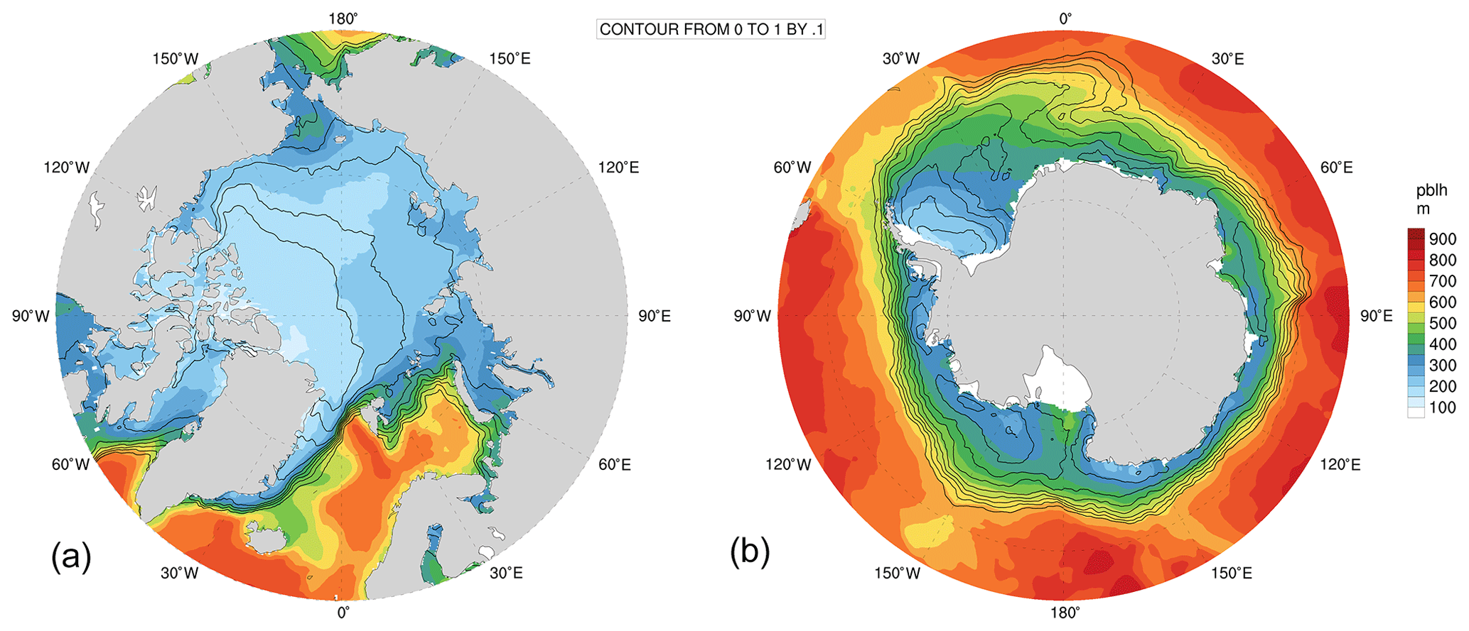
Figure 11Yearly average of sea-ice cover (contours) and atmospheric boundary layer height (shaded) over the antarctic (b) and arctic (a) regions.
5.2.3 MABL and sea-ice coupling
The last illustration of our implementation presented in this section is the coupling of ABL1d with sea ice. As described in Sect. 4.3, sea ice generally induces a shallow stably stratified boundary layer due to the near-surface air cooling. This increased vertical stability tends to reduce atmospheric turbulence, producing shallower ABL heights over sea ice. This relationship between sea-ice concentration and ABL height is clearly visible from Fig. 11 on both Arctic and Antarctic domains, where the ABL height follows a progressive decrease from about 800 to 200 m in the transition zone between the open ocean and fully ice-covered regions. This coupling between the ABL and sea ice have important effects on near-surface wind, temperature, and humidity, and consequently on sea-ice concentration evolution, which will need to be specifically assessed in future ABL-based studies.
6.1 Summary
A simplified atmospheric boundary layer (ABL) model has been developed and integrated to an oceanic model. This development is made with the objective to improve the representation of air–sea interactions in eddying oceanic models compared to the standard forcing strategy where the 10 m height atmospheric quantities are prescribed. For this preliminary study, the simplified ABL model takes the form of a single-column model including a turbulence scheme coupled to each oceanic grid point. A crucial hypothesis is that the dominant process at the characteristic scale of the oceanic mesoscale is the so-called downward mixing process which stems from a modulation of atmospheric turbulence by sea surface temperature (SST) anomalies. Our approach can be seen as an extended bulk approach: instead of prescribing atmospheric quantities at 10 m to compute air–sea fluxes via an atmospheric surface layer (ASL) parameterization, atmospheric quantities in the first few hundred meters are used to constrain an ABL model which provides 10 m atmospheric values to the ASL parameterization. An important point is that our modeling strategy keeps the computational efficiency and flexibility inherent to ocean-only modeling. Indeed, the overhead generally observed in terms of computational cost compared to the usual ASL forcing strategy is roughly 10 %, and half of this overhead is due to I/O operations since the ABL model is constrained by 3D atmospheric data. In this paper the key components of such an approach have been described. This includes the large-scale forcing strategy, the coupling with the ocean and sea ice and last but not least the ABL turbulence closure scheme based on a prognostic equation for the turbulence kinetic energy. The resulting simplified model, called ABL1d, has been tested for several boundary-layer regimes relevant to either ocean–atmosphere or sea-ice–atmosphere coupling. Results have systematically been evaluated against large eddy simulations (LESs). Furthermore we have investigated the behavior of the model to several parameters including the formulation of the mixing length and the turbulence model constants. First results from a global ABL1d-NEMO configuration show an excellent behavior in terms of wind–SST two-way coupling. A first analysis of the impact of the coupling with ABL1d from a physical viewpoint is presented in Brivoal et al. (2020).
6.2 Future work
Now that an adequate computational framework and an efficient turbulent scheme that can be operated for a reasonable computational overhead have been developed, the next step is to investigate the relevance of the single-column representation of the ABL selected for the present paper. Indeed, several studies have already shown that momentum vertical turbulent mixing, pressure gradient, Coriolis, and nonlinear advection are all important to the momentum balance in the marine atmospheric boundary layer at the vicinity of oceanic fronts (see for example Spall, 2007; Small et al., 2008; O'Neill et al., 2010). It is well known that the relative importance of those terms depends on the wind regime: for strong winds the vertical mixing is the dominant mechanism while for weak winds the pressure adjustment mechanism dominates. The current single-column approximation is based on the assumption that the balance is dominated by vertical turbulent mixing, and the effect of other terms is roughly represented by the geostrophic guide and/or the nudging term. The test case presented in Sect. 4.4 clearly illustrates the limitations of a single-column approach ignoring advective effects. However, before moving to more advanced formulations, our rationale was that the two main bottlenecks in terms of computational cost inherent to the ABL coupling strategy are the reading of 3D atmospheric data and the choice of ABL turbulent scheme. As a first step, we focused on those two aspects to assess whether or not our approach can be a viable option. Even if the justification of our model is not beyond reproach, it already brings an improvement compared to the ASL forcing strategy.
Several ways to improve the methodology presented here are currently under investigation. At a practical level, ways to lower the computational overhead due to I/O operations will be investigated using the parallel I/O capabilities provided by the XIOS library which is currently used in NEMO only for outputs. At a more fundamental level, the continuous formulation of the ABL1d model will be completed to improve the representation of the momentum balance by integrating the effect of horizontal advection and fine-scale pressure gradients. Increasing the complexity of the model should allow the impact of the nudging term on the ABL solutions to be lowered. In the event our approach turns out to be physically sound for a reasonable complexity it could be useful not only for offline oceanic simulations but also in coupled simulations to downscale the information from a low-resolution atmospheric component to a high-resolution oceanic component. A standalone ABL model of intermediate complexity could also play a role in coupled data assimilation where the current practice is generally to assimilate data separately in the ocean and the atmosphere, ignoring the air–sea interactions, which results in inconsistencies at the air–sea interface in the initial conditions, causing initial shocks in the coupled forecasts (e.g., Mulholland et al., 2015). We wish to conclude this study by clarifying that the framework we have developed within NEMO is general enough to allow alternative approaches (e.g., via model-driven empirical models) to be seamlessly tested and confronted with the ABL coupling strategy.
In this appendix, following the methodology of Redelsperger et al. (2001) re-expressed with our notations, we quickly recall how the surface boundary conditions for the turbulent kinetic energy (TKE) and for the mixing lengths lm and lε are determined via a matching between the subgrid turbulence scheme and the surface-layer theory. The simplest form of atmospheric surface layer (ASL) theory, namely for neutral stratification, is considered. Under the quasi-equilibrium hypothesis the evolution Eq. (6) for the TKE reduces to the equilibrium between turbulence production and dissipation which, combined with , leads to
The similarity theory for the ASL in the neutral case is such that with κ the Von Karman constant and z0 the roughness length which can be combined with Eq. (A1) to get that in the surface layer:
with the friction velocity. Moreover, enforcing the consistency between the eddy diffusivity for momentum given by the ASL theory () and the one given by the TKE closure () leads to
We thus have two relations (A2) and (A3) for three unknowns (e, lm, and lε). At this point our derivation will differ from Redelsperger et al. (2001) as we will assume that in the ASL.
Under this assumption, combining Eqs. (A2) and (A3) we easily obtain
for z≤δasl, where δasl corresponds to the extent of the ASL.
The expression of Lsfc(z) for z≤δasl is also used as a constraint to define the weighted average needed to determine lm from lup and ldwn:
(equivalent to Eq. 12a). In the ASL we further assume that ldwn≈0 and lup≈δasl; for lm(z=δasl) to be consistent with Lsfc(z=δasl) we should have
Considering that δasl≫z0, Eq. (A4) is satisfied for
Considering the CBR00 model constants we obtain and for the CCH02 constants (see Table 1).
B1 Altitude of IFS vertical levels
The ABL1d model is discretized on fixed in time and space geopotential levels while the IFS model uses a pressure-based sigma coordinate. A first step is to recover the altitude associated with each sigma level. The pressure pk+½ defined at cell interfaces between two successive vertical layers is given by
where Ak+½ (Pa) and Bk+½ (dimensionless) are constants given by a smooth analytical function defining the vertical grid stretching. Typical values of the altitude of grid points in the vertical for a standard 60-level grid (L60) and a surface pressure of 1013 hPa are given in Table B1. Once the values of pk+½ and ps are known, the altitude of cell interfaces can be computed by integrating the hydrostatic equilibrium
vertically. In Eq. (B1), ϕ is the geopotential, Tv the virtual temperature, and Rd the specific gas constant for dry air. At a discrete level we get
which gives
Once the layer thicknesses are known, horizontal wind components, potential temperature, and specific humidity can be interpolated on the ABL1d vertical levels. Under the constraint that for any IFS quantity ψifs to be interpolated. Wind components are interpolated using a fourth-order compact scheme while tracers are interpolated using a WENO-like PPM scheme (Alexander Shchepetkin, personal communication, 2001) which is monotonic.
Table B1Altitude zk and layer thickness e3tk of the IFS L60 vertical grid in the first 2000 m with respect to the parameter values Ak and Bk of a surface pressure ps=1013 hPa.
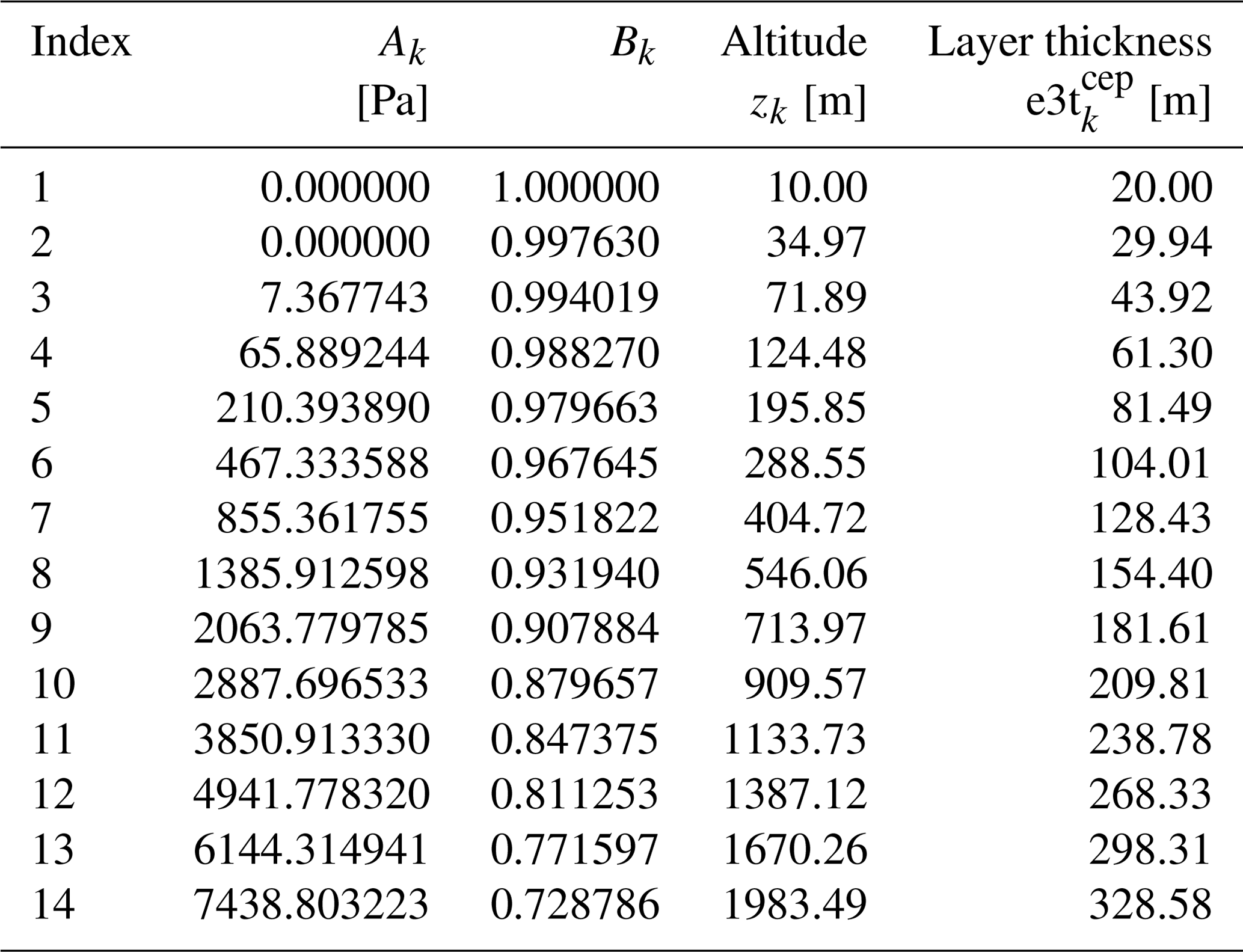
B2 Filtering in the presence of boundaries
Because of the IFS numerical formulation and of the post-processing of output data, the solutions sometimes contain high-frequency oscillations at the vicinity of the land-sea interface. This problem is further compounded when the nearshore topography is steep. The atmospheric fields over water thus need to be smoothed horizontally to specifically remove the 2Δx noise. We use a standard two-dimensional Shapiro filter which, in the absence of lateral boundaries, can be formulated as
where and . The amplification factor associated with this filter is
which guarantees that one iteration of the filter is sufficient to remove the grid-scale noise since and that 𝒜shap≤1 (i.e., no waves are amplified). In the presence of solid boundaries we would like to retain those properties as much as possible. A straightforward approach would be to impose a no-gradient condition at the coast, i.e., as soon as ( as soon as ), with tmask the indicator function equal to 1 over water and 0 over land. Let us also consider the following alternative boundary conditions
and similar in the y direction. We do not elaborate on this choice but it can be shown theoretically that boundary conditions (B2) provide a better control of grid-scale noise near the coast. To illustrate this point, in Fig. B1 the surface pressure gradients are shown for different boundary conditions. In particular it can be seen near the coast that the no-gradient boundary condition (panels b and e) leaves some artificial patterns in gradients, especially in the Peru–Chile current system, while the boundary condition (B2) efficiently mitigates this issue. Note that it is particularly essential to make sure that the surface pressure field is sufficiently smooth because gradients of this field are used to compute geostrophic winds which are important for the large-scale forcing of the ABL1d model.
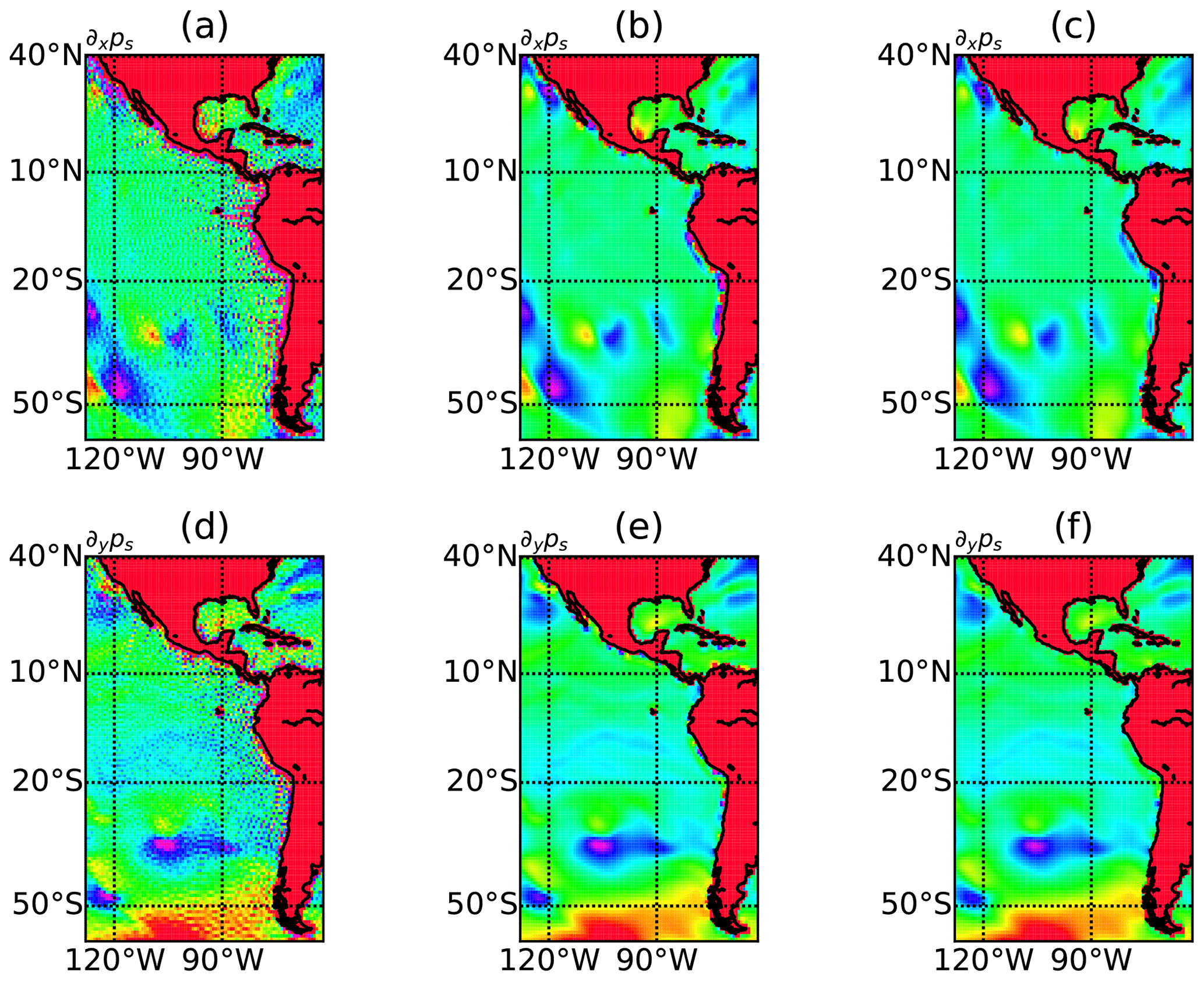
Figure B1Atmospheric surface pressure horizontal gradients in x (a, b, c) and y (d, e, f) directions obtained from the original IFS data (a, d), after a Shapiro filtering with no-gradient boundary conditions (b, e), and after a Shapiro filtering with boundary conditions (B2) (c, f). The area in red is covered by land.
B3 Large-scale pressure gradient computation
The last aspect of the pre-processing of atmospheric data we would like to discuss is the computation of the large-scale pressure gradient (or equivalently of the geostrophic wind components) The objective is to estimate the following terms:
where (⋅)z denotes a gradient along constant geopotential height. Using the hydrostatic balance we have , which leads to
Assuming a generalized vertical coordinate the computation of gradients along constant height is not straightforward since leading to
In the particular case of the IFS coordinate s we have
and (∂xz)s can be estimated after integrating the hydrostatic balance. Starting from the layer interface height , surface pressure (ps)i,j, and parameter values the different steps are the following:
-
compute Δxi,j and Δyi,j from latitudes and longitudes;
-
compute horizontal gradients ∂xps and ∂yps for surface pressure
-
compute horizontal gradients (∂xz)s and (∂yz)s
-
compute via (B4)
-
finalize (we get a minus sign in because the grid in the y direction is flipped in the raw data)
In the following we describe the discrete algorithms used to provide the mixing lengths lup and ldwn given in Sect. 3.2.2. Four different ways to compute those quantities have been implemented in the ABL1d model.
C1 Bougeault and Lacarrère (1989) length scale
The Bougeault and Lacarrère (1989) mixing length defines lup and ldwn as
By construction such mixing lengths are bounded by the distance to the bottom and the top of the computational domain and revert to the Deardorff (1980) length scale (i.e., ) for N2=cste. An objective is to also satisfy this last property at a discrete level. Considering a simple trapezoidal rule to approximate the integral in Eq. (C1) over each grid cell, the procedure for the computation of is given in Algorithm 1. In the case , Algorithm 1 gives the following sequence:
As soon as changes sign we stop the procedure
because lup such that
, which corresponds
to the Deardorff (1980) length scale, has been found.
We note lBL89 the mixing length corresponding to the
Bougeault and Lacarrère (1989) algorithm.
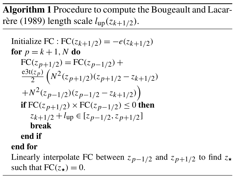
C2 Adaptation of NEMO's length scale
The standard NEMO algorithm (Sect. 10.1.3 in Madec, 2012) is much easier to discretize. As a first step the Deardorff (1980) length scale lD80 is computed at cell interfaces, such that
with the minimum stratification allowed whose value is set to the smallest positive real computer value. The vertical gradients of lD80 are then limited such that they stay smaller than the variations of height. This amounts to compute lup and ldwn as
with e3tk the thickness of vertical layer k (Fig. 2). The resulting mixing length is simply referred to as lD80.
C3 Rodier et al. (2017) length scale
Recently, Rodier et al. (2017) proposed to add a shear-related term to Eq. (C1) such that the definition of lup and ldwn becomes
where c0 is a parameter whose value should be smaller than . At a discrete level, the FC function in Algorithm 1 is replaced by
This mixing length will be referred to as lR17.
C4 A local buoyancy- and shear-based length scale
For the sake of computational efficiency, we have derived a local version of the Rodier et al. (2017) length scale (denoted as ) which is original to the present paper:
Once has been computed at cell interfaces we apply the limitations (C2) and (C3) as in the NEMO algorithm.
To finalize our description of the implementation of the simplified atmospheric boundary layer model in NEMO, we assess in this appendix the computational efficiency of our approach. We compare the performance of two simulations: one with a coupling with the ABL1d model (with 50 vertical levels) which requires reading 3D atmospheric data in input files, and one with a standard ASL forcing strategy which necessitates reading only 2D atmospheric data. For the coupling with ABL1d, we consider the lD80 mixing length which gave robustly good results across the different numerical tests investigated earlier in the paper. The simulations are performed with NEMO version 4.0 for the ORCA025 configuration previously described on 128 cores (Intel(R) Xeon(R) E5 processors 2.6 GHz) compiled with ifort (v13.0.1) using the “” options. The I/Os are handled via the Lustre file system. Each MPI subdomain has 80×130 points in the horizontal and 75 points in the vertical. The various reports given below have been obtained from a built-in NEMO code instrumentation dedicated to calculation measurement (e.g., Maisonnave and Masson, 2019). As mentioned earlier, the outputs are done using the parallel I/O capabilities provided by the XIOS library. Thanks to XIOS, we do not expect any significant difference between the two simulations regarding the cost of output operations. However, the use of XIOS to handle input operations is still under development, and because of the significant amount of data to read in the ABL coupling strategy it makes sense to assess the associated overhead. We ran the ASL forced and ABL coupled NEMO simulations for 20 d such that the cost of the initialization step is no longer visible in the averaged cost per time step. Moreover, for the two simulations, the atmospheric data necessary for the computation of the turbulent components of air–sea fluxes are provided every 6 h.
We first show in Fig. D1 the elapsed time for each time step over the first 48 h of the simulations with different ways to specify the surface fluxes. For most time steps, the overhead associated with the ABL1d when using the lD80 mixing length is very small (on the order of 4 %); however, every 18 time steps (i.e., every 6 h), there is a larger overhead due to the input part of the I/O operations. To further refine our assessment, we report in Table D1 the elapsed and CPU time spent on average over all the processors in the 11 most expansive sections of the code. As expected, the CPU time is not significantly affected by the ABL1d model (increase of 4 %), but the elapsed time is increased by about 9 % because of the time spent in waiting for I/O operations. The overhead associated with input operations could be mitigated by reducing the number of vertical levels in the ABL1d model (we used 50 levels here to get an upper bound on the computational overhead) and either by using XIOS to handle input operations or by running ABL1d in detached mode as explained in Sect. 3.4 such that the time spent reading input files is covered by actual computations. Nonetheless the small increase in CPU time leaves room for further improvements of the ABL model to relax the horizontal homogeneity assumption.
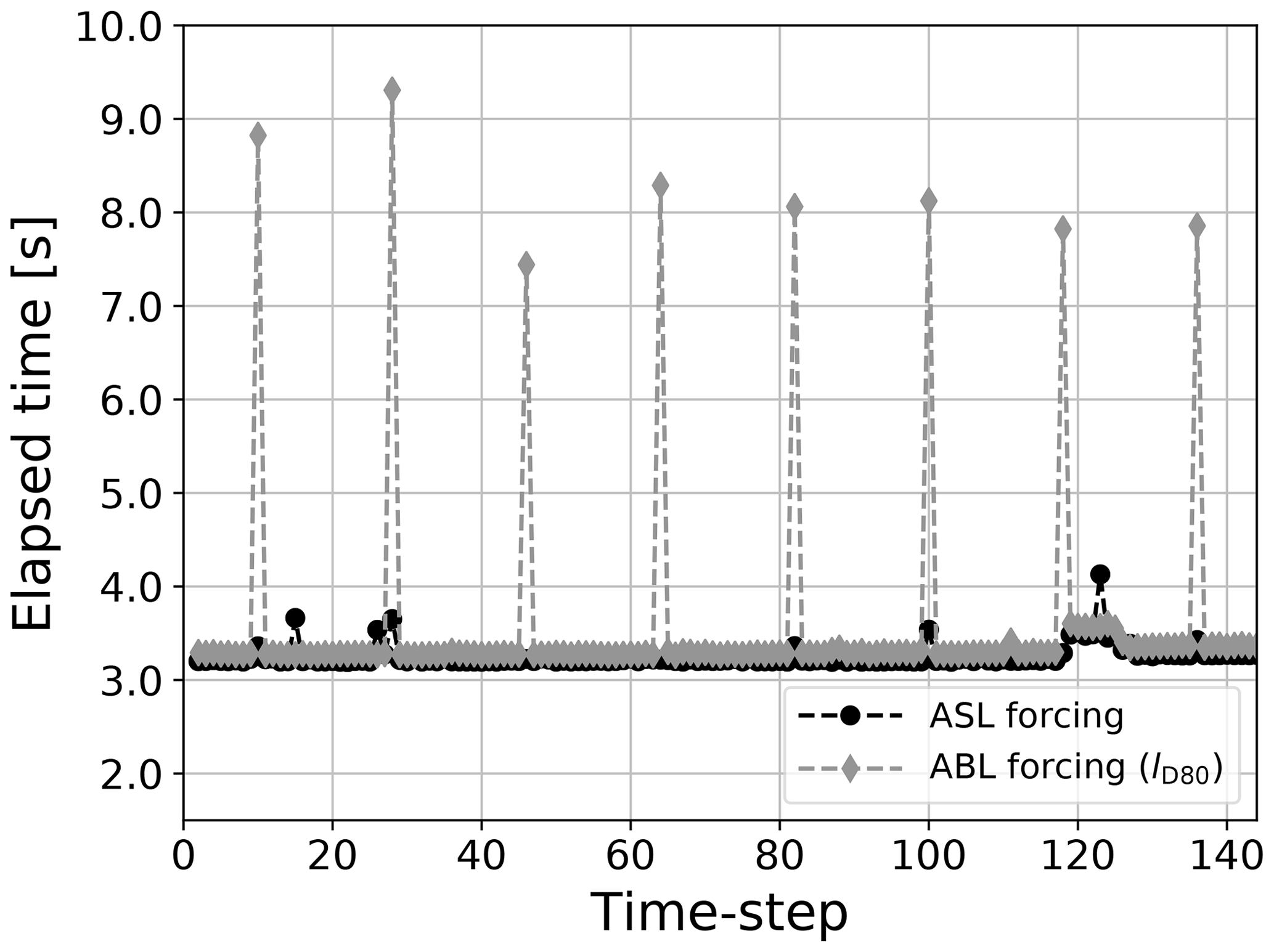
Figure D1Elapsed time for each time step of a 48 h simulation with standard ASL forcing strategy (black circles) and ABL forcing strategy using the lD80 mixing length (gray diamonds). For the two simulations the time step size is Δt=1200 s.
Table D1Report of the elapsed time and CPU time in different sections of the NEMO (v4.0) code for the ASL forcing strategy (left portion of the table) and the ABL coupling strategy (right portion of the table). The timing is averaged on all processors. The right-most column provides a quick description of the task handled by the corresponding section. On top of the timing in seconds the percentage of the total CPU and elapsed time associated with each section is reported in parentheses. The computational overhead associated with the ABL coupling strategy can be estimated from the sbc section and the elapsed and CPU time.
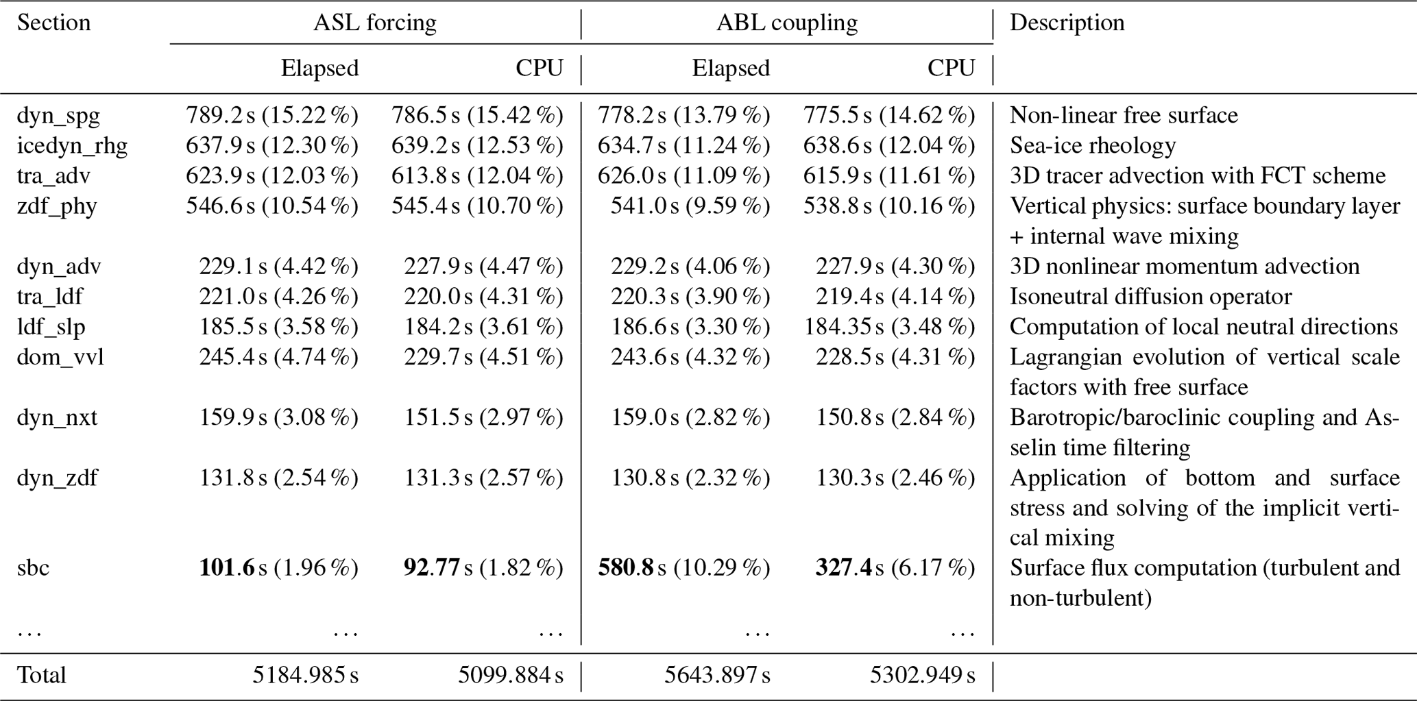
The changes to the NEMO code have been made on the standard NEMO code (release 4.0). The code can be downloaded from the NEMO website (http://www.nemo-ocean.eu/, last access: 23 June 2020). The NEMO code modified to include the ABL1d model is available in the Zenodo archive (https://doi.org/10.5281/zenodo.3904518, Lemarié and Samson, 2020). The name lists and data used to produce the figures are also available in the Zenodo archive.
FL wrote the paper with the help of all the coauthors. FL, GS, and GM designed and developed a preliminary version of the ABL1d model within the NEMO 3.6 stable version. This original code was then ported to NEMO release 4.0. JLR and HG provided inputs in the design of the TKE closure scheme and of the numerical experiments. FL carried out the idealized numerical experiments, GS the realistic experiments, and JLR the MesoNH simulations.
The authors declare that they have no conflict of interest.
We thank Anton Beljaars and one anonymous reviewer whose efforts helped to improve earlier versions of this paper. We also thank Pascal Marquet and Sébastien Masson for useful discussions.
Florian Lemarié and Jean-Luc Redelsperger also acknowledge the support by Mercator-Ocean and the Copernicus Marine Environment Monitoring Service (CMEMS) through contract 22-GLO-HR – Lot 2 (High-resolution ocean, waves, atmosphere interaction).
This research has been supported by the H2020 European Institute of Innovation and Technology (IMMERSE (grant no. 821926)).
This paper was edited by Christina McCluskey and reviewed by Anton Beljaars and one anonymous referee.
Abel, R.: Aspects of air-sea interaction in atmosphere-ocean models, PhD thesis, Kiel University, 2018. a
Andren, A., Brown, A. R., Mason, P. J., Graf, J., Schumann, U., Moeng, C.-H., and Nieuwstadt, F. T. M.: Large-eddy simulation of a neutrally stratified boundary layer: A comparison of four computer codes, Q. J. Roy. Meteor. Soc., 120, 1457–1484, 1994. a, b, c, d
Ayet, A. and Redelsperger, J.-L.: An analytical study of the atmospheric boundary layer flow and divergence over a SST front, Q. J. Roy. Meteor. Soc., 145, 2549–2567, https://doi.org/10.1002/qj.3578, 2019. a, b, c, d
Baklanov, A. A., Grisogono, B., Bornstein, R., Mahrt, L., Zilitinkevich, S. S., Taylor, P., Larsen, S. E., Rotach, M. W., and Fernando, H. J. S.: The Nature, Theory, and Modeling of Atmospheric Planetary Boundary Layers, B. Am. Meteorol. Soc., 92, 123–128, https://doi.org/10.1175/2010BAMS2797.1, 2011. a
Barnier, B., Siefridt, L., and Marchesiello, P.: Thermal forcing for a global ocean circulation model using a three-year climatology of ECMWF analyses, J. Mar. Res., 6, 363–380, https://doi.org/10.1016/0924-7963(94)00034-9, 1995. a
Barnier, B., Madec, G., Penduff, T., Molines, J.-M., Treguier, A.-M., Le Sommer, J., Beckmann, A., Biastoch, A., Böning, C., Dengg, J., Derval, C., Durand, E., Gulev, S., Remy, E., Talandier, C., Theetten, S., Maltrud, M., McClean, J., and De Cuevas, B.: Impact of partial steps and momentum advection schemes in a global ocean circulation model at eddy-permitting resolution, Ocean Dynam., 56, 543–567, https://doi.org/10.1007/s10236-006-0082-1, 2006. a
Bazile, E., Marquet, P., Bouteloup, Y., and Bouyssel, F.: The Turbulent Kinetic Energy (TKE) scheme in the NWP models at Meteo France, in: Workshop on Workshop on Diurnal cycles and the stable boundary layer, 7–10 November 2011, ECMWF, Shinfield Park, Reading, 127–135, available at: https://www.ecmwf.int/node/8006 (last access: 20 January 2021), 2012. a, b
Beljaars, A.: The parametrization of surface fluxes in large-scale models under free convection, Q. J. Roy. Meteor. Soc., 121, 255–270, 1995. a
Beljaars, A., Dutra, E., Balsamo, G., and Lemarié, F.: On the numerical stability of surface–atmosphere coupling in weather and climate models, Geosci. Model Dev., 10, 977–989, https://doi.org/10.5194/gmd-10-977-2017, 2017. a, b
Bielli, S., Douville, H., and Pohl, B.: Understanding the West African monsoon variability and its remote effects: An illustration of the grid point nudging methodology, Clim. Dynam., 35, 159–174, https://doi.org/10.1007/s00382-009-0667-8, 2009. a
Bougeault, P. and André, J.-C.: On the Stability of the THIRD-Order Turbulence Closure for the Modeling of the Stratocumulus-Topped Boundary Layer, J. Atmos. Sci., 43, 1574–1581, https://doi.org/10.1175/1520-0469(1986)043<1574:OTSOTT>2.0.CO;2, 1986. a
Bougeault, P. and Lacarrère, P.: Parameterization of orography-induced turbulence in a mesobeta-scale model, Mon. Weather Rev., 117, 1872–1890, 1989. a, b, c, d, e, f
Bourras, D., Reverdin, G., Giordani, H., and Caniaux, G.: Response of the atmospheric boundary layer to a mesoscale oceanic eddy in the northeast Atlantic, J. Geophys. Res., 109, https://doi.org/10.1029/2004JD004799, 2004. a
Brivoal, T., Samson, G., Giordani, H., Bourdallé-Badie, R., Lemarié, F., and Madec, G.: Impact of the current feedback on kinetic energy over the North-East Atlantic from a coupled ocean/atmospheric boundary layer model, Ocean Sci. Discuss. [preprint], https://doi.org/10.5194/os-2020-78, in review, 2020. a
Brodeau, L., Barnier, B., Gulev, S. K., and Woods, C.: Climatologically Significant Effects of Some Approximations in the Bulk Parameterizations of Turbulent Air–Sea Fluxes, J. Phys. Oceanogr., 47, 5–28, https://doi.org/10.1175/JPO-D-16-0169.1, 2017. a
Bryan, F. O., Tomas, R., Dennis, J. M., Chelton, D. B., Loeb, N. G., and McClean, J. L.: Frontal Scale Air–Sea Interaction in High-Resolution Coupled Climate Models, J. Climate, 23, 6277–6291, https://doi.org/10.1175/2010JCLI3665.1, 2010. a, b, c, d
Burchard, H.: Energy-conserving discretisation of turbulent shear and buoyancy production, Ocean Modell., 4, 347–361, https://doi.org/10.1016/S1463-5003(02)00009-4, 2002a. a
Burchard, H.: Applied Turbulence Modelling in Marine Waters, Lecture Notes in Earth Sciences, Springer Berlin Heidelberg, 2002b. a, b
Businger, J. and Shaw, W.: The response of the marine boundary layer to mesoscale variations in sea-surface temperature, Dynam. Atmos. Oceans, 8, 267–281, 1984. a
Chelton, D. B. and Xie, S.-P.: Coupled ocean-atmosphere interaction at oceanic mesoscales, Oceanography, 23, 52–69, 2010. a, b, c
Cheng, Y., Canuto, V. M., and Howard, A. M.: An improved model for the turbulent PBL, J. Atmos. Sci., 59, 1550–1565, 2002. a, b, c, d, e
Couvelard, X., Lemarié, F., Samson, G., Redelsperger, J.-L., Ardhuin, F., Benshila, R., and Madec, G.: Development of a two-way-coupled ocean–wave model: assessment on a global NEMO(v3.6)–WW3(v6.02) coupled configuration, Geosci. Model Dev., 13, 3067–3090, https://doi.org/10.5194/gmd-13-3067-2020, 2020. a
Craig, A., Valcke, S., and Coquart, L.: Development and performance of a new version of the OASIS coupler, OASIS3-MCT_3.0, Geosci. Model Dev., 10, 3297–3308, https://doi.org/10.5194/gmd-10-3297-2017, 2017. a
Cuxart, J., Bougeault, P., and Redelsperger, J.-L.: A turbulence scheme allowing for mesoscale and large-eddy simulations, Q. J. Roy. Meteor. Soc., 126, 1–30, 2000. a, b, c, d, e, f, g, h, i
Cuxart, J., Holtslag, A. A. M., Beare, R. J., Bazile, E., Beljaars, A., Cheng, A., Conangla, L., Ek, M., Freedman, F., Hamdi, R., Kerstein, A., Kitagawa, H., Lenderink, G., Lewellen, D., Mailhot, J., Mauritsen, T., Perov, V., Schayes, G., Steeneveld, G.-J., Svensson, G., Taylor, P., Weng, W., Wunsch, S., and Xu, K.-M.: Single-Column Model Intercomparison for a Stably Stratified Atmospheric Boundary Layer, Bound.-Lay. Meteorol., 118, 273–303, 2006. a, b, c
Deardorff, J. W.: Three-dimensional numerical study of turbulence in an entraining mixed layer, Bound.-Lay. Meteorol., 7, 199–226, 1974. a
Deardorff, J. W.: Stratocumulus-capped mixing layers derived from a three dimensional model, Bound.-Lay. Meteorol., 18, 495–527, 1980. a, b, c, d, e, f
Dee, D. P., Uppala, S. M., Simmons, A. J., Berrisford, P., Poli, P., Kobayashi, S., Andrae, U., Balmaseda, M. A., Balsamo, G., Bauer, P., Bechtold, P., Beljaars, A. C. M., van de Berg, L., Bidlot, J., Bormann, N., Delsol, C., Dragani, R., Fuentes, M., Geer, A. J., Haimberger, L., Healy, S. B., Hersbach, H., Hólm, E. V., Isaksen, L., Kållberg, P., Köhler, M., Matricardi, M., McNally, A. P., Monge-Sanz, B. M., Morcrette, J.-J., Park, B.-K., Peubey, C., de Rosnay, P., Tavolato, C., Thépaut, J.-N., and Vitart, F.: The ERA-Interim reanalysis: configuration and performance of the data assimilation system, Q. J. Roy. Meteor. Soc., 137, 553–597, https://doi.org/10.1002/qj.828, 2011. a
Deleersnijder, E., Beckers, J.-M., Campin, J.-M., El Mohajir, M., Fichefet, T., and Luyten, P.: Some mathematical problems associated with the development and use of marine models, in: The Mathematics of Models for Climatology and Environment, edited by: Díaz, J. I., Springer Berlin Heidelberg, Berlin, Heidelberg, 39–86, 1997. a
Deremble, B., Wienders, N., and Dewar, W. K.: CheapAML: A Simple, Atmospheric Boundary Layer Model for Use in Ocean-Only Model Calculations, Mon. Weather Rev., 141, 809–821, 2013. a
Deshayes, J., Tréguier, A.-M., Barnier, B., Lecointre, A., Sommer, J. L., Molines, J.-M., Penduff, T., Bourdallé-Badie, R., Drillet, Y., Garric, G., Benshila, R., Madec, G., Biastoch, A., Böning, C. W., Scheinert, M., Coward, A. C., and Hirschi, J. J.-M.: Oceanic hindcast simulations at high resolution suggest that the Atlantic MOC is bistable, J. Geophys. Res., 40, 3069–3073, https://doi.org/10.1002/grl.50534, wOS:000321951300034, 2013. a
Dewar, W. K. and Flierl, G. R.: Some Effects of the Wind on Rings, J. Phys. Oceanogr., 17, 1653–1667, 1987. a
Frenger, I., Gruber, N., Knutti, R., and Munnich, M.: Southern Ocean Eddies Affect Local Weather, Nat. Geosci., 6, 608–612, 2013. a
Giordani, H., Planton, S., Bénech, B., and Kwon, B.-H.: Atmospheric boundary layer response to sea surface temperatures during the Semaphore experiment, J. Geophys. Res., 103, 25047–25060, 1998. a
Giordani, H., Caniaux, G., and Prieur, L.: A Simplified 3D Oceanic Model Assimilating Geostrophic Currents: Application to the POMME Experiment, J. Phys. Oceanogr., 35, 628–644, https://doi.org/10.1175/JPO2724.1, 2005. a
Haney, R. L.: Surface Thermal Boundary Condition for Ocean Circulation Models, J. Phys. Oceanogr., 1, 241–248, https://doi.org/10.1175/1520-0485(1971)001<0241:STBCFO>2.0.CO;2, 1971. a
Hogg, A., Dewar, W., Berloff, P., Kravtsov, S., and Hutchinson, D. K.: The effects of mesoscale ocean-atmosphere coupling on the large-scale ocean circulation, J. Climate, 22, 4066–4082, 2009. a
Hourdin, F., Couvreux, F., and Menut, L.: Parameterization of the Dry Convective Boundary Layer Based on a Mass Flux Representation of Thermals, J. Atmos. Sci., 59, 1105–1123, https://doi.org/10.1175/1520-0469(2002)059<1105:POTDCB>2.0.CO;2, 2002. a
Kilpatrick, T., Schneider, N., and Qiu, B.: Boundary Layer Convergence Induced by Strong Winds across a Midlatitude SST Front, J. Climate, 27, 1698–1718, 2014. a, b, c
Kleeman, R. and Power, S.: A Simple Atmospheric Model of Surface Heat Flux for Use in Ocean Modeling Studies, J. Phys. Oceanogr., 25, 92–105, https://doi.org/10.1175/1520-0485(1995)025<0092:ASAMOS>2.0.CO;2, 1995. a
Lac, C., Chaboureau, J.-P., Masson, V., Pinty, J.-P., Tulet, P., Escobar, J., Leriche, M., Barthe, C., Aouizerats, B., Augros, C., Aumond, P., Auguste, F., Bechtold, P., Berthet, S., Bielli, S., Bosseur, F., Caumont, O., Cohard, J.-M., Colin, J., Couvreux, F., Cuxart, J., Delautier, G., Dauhut, T., Ducrocq, V., Filippi, J.-B., Gazen, D., Geoffroy, O., Gheusi, F., Honnert, R., Lafore, J.-P., Lebeaupin Brossier, C., Libois, Q., Lunet, T., Mari, C., Maric, T., Mascart, P., Mogé, M., Molinié, G., Nuissier, O., Pantillon, F., Peyrillé, P., Pergaud, J., Perraud, E., Pianezze, J., Redelsperger, J.-L., Ricard, D., Richard, E., Riette, S., Rodier, Q., Schoetter, R., Seyfried, L., Stein, J., Suhre, K., Taufour, M., Thouron, O., Turner, S., Verrelle, A., Vié, B., Visentin, F., Vionnet, V., and Wautelet, P.: Overview of the Meso-NH model version 5.4 and its applications, Geosci. Model Dev., 11, 1929–1969, https://doi.org/10.5194/gmd-11-1929-2018, 2018. a
Lafore, J. P., Stein, J., Asencio, N., Bougeault, P., Ducrocq, V., Duron, J., Fischer, C., Héreil, P., Mascart, P., Masson, V., Pinty, J. P., Redelsperger, J. L., Richard, E., and Vilà-Guerau de Arellano, J.: The Meso-NH Atmospheric Simulation System. Part I: adiabatic formulation and control simulations, Ann. Geophys., 16, 90–109, 1998. a
Lambaerts, J., Lapeyre, G., Plougonven, R., and Klein, P.: Atmospheric response to sea surface temperature mesoscale structures, J. Geophys. Res., 118, 9611–9621, 2013. a
Large, W. G.: Surface Fluxes for Practitioners of Global Ocean Data Assimilation, in: Ocean Weather Forecasting. An Integrated View of Oceanography, edited by: Chassignet, E. P. and Verron, J., chap. 9, Springer, 229–270, 2006. a
Large, W. G. and Yeager, S. G.: The global climatology of an interannually varying air-sea flux data set, Clim. Dynam., 33, 341–364, https://doi.org/10.1007/s00382-008-0441-3, 2009. a
Lemarié, F. and Samson, G.: A simplified atmospheric boundary layer model for an improved representation of air-sea interactions in eddying oceanic models: implementation and first evaluation in NEMO (v4.0)), Zenodo, https://doi.org/10.5281/zenodo.3904518, 2020. a, b
Lemarié, F., Kurian, J., Shchepetkin, A. F., Molemaker, M. J., Colas, F., and McWilliams, J. C.: Are there inescapable issues prohibiting the use of terrain-following coordinates in climate models?, Ocean Modell., 42, 57–79, https://doi.org/10.1016/j.ocemod.2011.11.007, 2012. a
LeMone, M. A., Angevine, W. M., Bretherton, C. S., Chen, F., Dudhia, J., Fedorovich, E., Katsaros, K. B., Lenschow, D. H., Mahrt, L., Patton, E. G., Sun, J., Tjernström, M., and Weil, J.: 100 Years of Progress in Boundary Layer Meteorology, Meteorol. Monogr., 59, 9.1–9.85, https://doi.org/10.1175/AMSMONOGRAPHS-D-18-0013.1, 2019. a, b
Lilly, D.: The representation of small-scale turbulence in numerical simulation experiments, in: Proc. IBM Sci. Comput. Symp. on Environmental Sci., 14–16 November 1966, Thomas J. Watson Res. Center, Yorktown Heights, N. Y., IBM Form 320–1951, 195–210, 1967. a
Lindzen, R. S. and Nigam, S.: On the role of sea surface temperature gradients in forcing low-level winds and convergence in the tropics, J. Atmos. Sci., 44, 2418–2436, 1987. a
Madec, G.: NEMO ocean engine, in: Note du Pole de modélisation No. 27, Institut Pierre-Simon Laplace (IPSL), France, 2012. a, b, c
Maisonnave, E. and Masson, S.: Ocean/sea-ice macro task parallelism in NEMO, in: Technical report, TR/GMGC/15/54, available at: https://www.cerfacs.fr/~maisonna/Reports/opa_sas_tr.pdf (last access: 20 January 2021), 2015. a
Maisonnave, E. and Masson, S.: NEMO 4.0 performance: how to identify and reduce unnecessary communications, in: Technical report, TR/CMGC/19/19, available at: https://cerfacs.fr/wp-content/uploads/2019/01/GLOBC-TR_Maisonnave-Nemo-2019.pdf (last access: 20 January 2021), 2019. a
Marchesiello, P., Capet, X., Menkes, C., and Kennan, S.: Submesoscale dynamics in tropical instability waves, Ocean Modell., 39, 31–46, https://doi.org/10.1016/j.ocemod.2011.04.011, 2011. a
McWilliams, J. C., Gula, J., and Molemaker, M. J.: The Gulf Stream North Wall: Ageostrophic Circulation and Frontogenesis, J. Phys. Oceanogr., 49, 893–916, https://doi.org/10.1175/JPO-D-18-0203.1, 2019. a
Metzger, E. J., Smedstad, O. M., Thoppil, P. G., Hurlburt, H. E., Cummings, J. A., Wallcraft, A. J., Zamudio, L., Franklin, D. S., Posey, P. G., Phelps, M. W., Hogan, P. J., Bub, F. L., and DeHaan, C. J.: US Navy Operational Global Ocean and Arctic Ice Prediction Systems, Oceanogr., 27, 32–43, https://doi.org/10.5670/oceanog.2014.66, 2014. a
Meurdesoif, Y., Caubel, A., Lacroix, R., Dérouillat, J., and Nguyen, M.: XIOS Tutorial, available at: http://forge.ipsl.jussieu.fr/ioserver/raw-attachment/wiki/WikiStart/XIOS-tutorial.pdf (last access: 20 January 2021), 2016. a
Minobe, S., Kuwano-Yoshida, A., Komori, N., Xie, S.-P., and Small, R. J.: Influence of the Gulf Stream on the troposphere, Nature, 452, 206–209, 2008. a
Monin, A. S. and Obukhov, A. M.: Basic laws of turbulent mixing in the surface layer of the atmosphere, Trudy Akademii Nauk SSSR Geofizicheskogo Instituta, 24, 163–187, 1954. a
Mulholland, D. P., Laloyaux, P., Haines, K., and Balmaseda, M. A.: Origin and Impact of Initialization Shocks in Coupled Atmosphere-Ocean Forecasts, Mon. Weather Rev., 143, 4631–4644, https://doi.org/10.1175/MWR-D-15-0076.1, 2015. a, b
Oerder, V., Colas, F., Echevin, V., Masson, S., Hourdin, C., Jullien, S., Madec, G., and Lemarié, F.: Mesoscale SST–wind stress coupling in the Peru–Chile current system: Which mechanisms drive its seasonal variability?, Clim. Dynam., 47, 2309–2330, 2016. a, b
O'Neill, L. W., Esbensen, S. K., Thum, N., Samelson, R. M., and Chelton, D. B.: Dynamical Analysis of the Boundary Layer and Surface Wind Responses to Mesoscale SST Perturbations, J. Climate, 23, 559–581, https://doi.org/10.1175/2009JCLI2662.1, 2010. a, b
Razavi, S., Tolson, B. A., and Burn, D. H.: Review of surrogate modeling in water resources, Water Resour. Res., 48, W07401, https://doi.org/10.1029/2011WR011527, 2012. a
Redelsperger, J. L., Mahé, F., and Carlotti, P.: A Simple And General Subgrid Model Suitable Both For Surface Layer And Free-Stream Turbulence, Bound.-Lay. Meteorol., 101, 375–408, 2001. a, b, c
Renault, L., Molemaker, M. J., Gula, J., Masson, S., and McWilliams, J. C.: Control and Stabilization of the Gulf Stream by Oceanic Current Interaction with the Atmosphere, J. Phys. Oceanogr., 46, 3439–3453, https://doi.org/10.1175/JPO-D-16-0115.1, 2016a. a
Renault, L., Molemaker, M. J., McWilliams, J. C., Shchepetkin, A. F., Lemarié, F., Chelton, D., Illig, S., and Hall, A.: Modulation of Wind Work by Oceanic Current Interaction with the Atmosphere, J. Phys. Oceanogr., 46, 1685–1704, 2016b. a, b
Renault, L., Lemarié, F., and Arsouze, T.: On the implementation and consequences of the oceanic currents feedback in ocean–atmosphere coupled models, Ocean Modell., 141, 101 423, https://doi.org/10.1016/j.ocemod.2019.101423, 2019a. a, b, c
Renault, L., Masson, S., Oerder, V., Jullien, S., and Colas, F.: Disentangling the Mesoscale Ocean-Atmosphere Interactions, J. Geophys. Res., 124, 2164–2178, https://doi.org/10.1029/2018JC014628, 2019b. a, b, c
Rodier, Q., Masson, V., Couvreux, F., and Paci, A.: Evaluation of a Buoyancy and Shear Based Mixing Length for a Turbulence Scheme, Front. Earth Sci., 5, 65, https://doi.org/10.3389/feart.2017.00065, 2017. a, b, c, d, e, f, g, h
Rotta, J.: Statistische theorie nichthomogener turbulenz, Z. Physik, 129, 547–572, 1951. a
Rousset, C., Vancoppenolle, M., Madec, G., Fichefet, T., Flavoni, S., Barthélemy, A., Benshila, R., Chanut, J., Levy, C., Masson, S., and Vivier, F.: The Louvain-La-Neuve sea ice model LIM3.6: global and regional capabilities, Geosci. Model Dev., 8, 2991–3005, https://doi.org/10.5194/gmd-8-2991-2015, 2015. a, b
Schneider, N. and Qiu, B.: The Atmospheric Response to Weak Sea Surface Temperature Fronts, J. Atmos. Sci., 72, 3356–3377, https://doi.org/10.1175/JAS-D-14-0212.1, 2015. a, b, c
Seager, R., Blumenthal, M. B., and Kushnir, Y.: An advective atmospheric mixed layer model for ocean modeling purposes: global simulation of surface heat fluxes, J. Climate, 8, 1952–1964, 1995. a
Small, R. J., deSzoeke, S. P., Xie, S. P., O'Neill, L., Seo, H., Song, Q., Cornillon, P., Spall, M., and Minobe, S.: Air-sea interaction over ocean fronts and eddies, Dynam. Atmos. Oceans, 45, 274–319, https://doi.org/10.1016/j.dynatmoce.2008.01.001, 2008. a
Soares, P. M. M., Miranda, P. M. A., Siebesma, A. P., and Teixeira, J.: An eddy-diffusivity/mass-flux parametrization for dry and shallow cumulus convection, Q. J. Roy. Meteor. Soc., 130, 3365–3383, https://doi.org/10.1256/qj.03.223, 2004. a
Spall, M.: Midlatitude Wind Stress–Sea Surface Temperature Coupling in the Vicinity of Oceanic Fronts, J. Climate, 20, 3785–3801, https://doi.org/10.1175/JCLI4234.1, 2007. a, b
Takano, K., Mintz, Y., and Han, J.-Y.: Numerical simulation of the world ocean circulation, Second Conf. on Numerical Weather Prediction, Monterey, CA, Amer. Meteor. Soc., 121–129, 1973. a
Troen, I. B. and Mahrt, L.: A simple model of the atmospheric boundary layer; sensitivity to surface evaporation, Bound.-Lay. Meteorol., 37, 129–148, https://doi.org/10.1007/BF00122760, 1986. a
von Schuckmann, K., Traon, P.-Y. L., Smith, N., Pascual, A., Brasseur, P., Fennel, K., Djavidnia, S., Aaboe, S., Fanjul, E. A., Autret, E., Axell, L., Aznar, R., Benincasa, M., Bentamy, A., Boberg, F., Bourdallé-Badie, R., Nardelli, B. B., Brando, V. E., Bricaud, C., Breivik, L.-A., Brewin, R. J., Capet, A., Ceschin, A., Ciliberti, S., Cossarini, G., de Alfonso, M., de Pascual Collar, A., de Kloe, J., Deshayes, J., Desportes, C., Drévillon, M., Drillet, Y., Droghei, R., Dubois, C., Embury, O., Etienne, H., Fratianni, C., Lafuente, J. G., Sotillo, M. G., Garric, G., Gasparin, F., Gerin, R., Good, S., Gourrion, J., Grégoire, M., Greiner, E., Guinehut, S., Gutknecht, E., Hernandez, F., Hernandez, O., Høyer, J., Jackson, L., Jandt, S., Josey, S., Juza, M., Kennedy, J., Kokkini, Z., Korres, G., Kõuts, M., Lagemaa, P., Lavergne, T., le Cann, B., Legeais, J.-F., Lemieux-Dudon, B., Levier, B., Lien, V., Maljutenko, I., Manzano, F., Marcos, M., Marinova, V., Masina, S., Mauri, E., Mayer, M., Melet, A., Mélin, F., Meyssignac, B., Monier, M., Müller, M., Mulet, S., Naranjo, C., Notarstefano, G., Paulmier, A., Gomez, B. P., Gonzalez, I. P., Peneva, E., Perruche, C., Peterson, K. A., Pinardi, N., Pisano, A., Pardo, S., Poulain, P.-M., Raj, R. P., Raudsepp, U., Ravdas, M., Reid, R., Rio, M.-H., Salon, S., Samuelsen, A., Sammartino, M., Sammartino, S., Sandø, A. B., Santoleri, R., Sathyendranath, S., She, J., Simoncelli, S., Solidoro, C., Stoffelen, A., Storto, A., Szerkely, T., Tamm, S., Tietsche, S., Tinker, J., Tintore, J., Trindade, A., van Zanten, D., Vandenbulcke, L., Verhoef, A., Verbrugge, N., Viktorsson, L., von Schuckmann, K., Wakelin, S. L., Zacharioudaki, A., and Zuo, H.: Copernicus Marine Service Ocean State Report, J. Oper. Oceanogr., 11, S1–S142, 2018. a
Wallace, J. M., Mitchell, T. P., and Deser, C.: The Influence of Sea-Surface Temperature on Surface Wind in the Eastern Equatorial Pacific: Seasonal and Interannual Variability, J. Climate, 2, 1492–1499, https://doi.org/10.1175/1520-0442(1989)002<1492:TIOSST>2.0.CO;2, 1989. a
Wilson, J. M. and Venayagamoorthy, S. K.: A Shear-Based Parameterization of Turbulent Mixing in the Stable Atmospheric Boundary Layer, J. Atmos. Sci., 72, 1713–1726, https://doi.org/10.1175/JAS-D-14-0241.1, 2015. a
This remark is supported by the conclusions of the CLIVAR Working Group on Model Development following the Kiel meeting in April 2014: http://www.clivar.org/sites/default/files/documents/exchanges65_0.pdf (last access: 20 January 2021)
However, we did not find significant differences in numerical solutions when using the following initial conditions:
- Abstract
- Introduction
- Model equations
- Numerical discretization and implementation within NEMO
- Atmosphere-only numerical experiments
- Coupled numerical experiments
- Conclusions
- Appendix A: Surface boundary conditions for TKE and mixing lengths
- Appendix B: Preprocessing of atmospheric data from IFS
- Appendix C: Discrete algorithms to compute lup and ldwn
- Appendix D: Code performance and profiling
- Code and data availability
- Author contributions
- Competing interests
- Acknowledgements
- Financial support
- Review statement
- References