Calibrating a global atmospheric chemistry transport model using Gaussian process emulation and ground-level concentrations of ozone and carbon monoxide

Atmospheric chemistry transport models are important tools to investigate the local, regional and global controls on atmospheric composition and air quality. To ensure that these models represent the atmosphere adequately, it is important to compare their outputs with measurements. However, ground based measurements of atmospheric composition are typically sparsely distributed and representative of much smaller spatial scales than those resolved in models; thus, direct comparison incurs uncertainty. In this study, we investigate the feasibility of using observations of one or more atmospheric constituents to estimate parameters in chemistry transport models and to explore how these estimates and their uncertainties depend upon representation errors and the level of spatial coverage of the measurements. We apply Gaussian process emulation to explore the model parameter space and use monthly averaged ground-level concentrations of ozone (O₃) and carbon monoxide (CO) from across Europe and the US. Using synthetic observations, we find that the estimates of parameters with greatest influence on O₃ and CO are unbiased, and the associated parameter uncertainties are low even at low spatial coverage or with high representation error. Using reanalysis data, we find that estimates of the most influential parameter – corresponding to the dry deposition process – are closer to its expected value using both O₃ and CO data than using O₃ alone. This is remarkable because it shows that while CO is largely unaffected by dry deposition, the additional constraints it provides are valuable for achieving unbiased estimates of the dry deposition parameter. In summary, these findings identify the level of spatial representation error and coverage needed to achieve good parameter estimates and highlight the benefits of using multiple constraints to calibrate atmospheric chemistry transport models.

1 Introduction

Changes in atmospheric composition due to human activities make an important contribution to Earth's changing climate (Stocker, 2013) and to outdoor air pollution, which is currently responsible for about 4.2 million deaths worldwide each year (Cohen et al., 2017), with 365 000 deaths due to surface ozone (DeLang et al., 2021). Chemistry transport models (CTMs) simulate the production, transport and removal of key atmospheric constituents, and they are important tools for understanding variations in atmospheric composition across space and time. They permit investigation of future climate and emission scenarios that fully account for the interactions and feedbacks that characterise physical, chemical and dynamical processes in the atmosphere. For practical application, CTMs need to reproduce the magnitude and variation in pollutant concentrations observed at a wide range of measurement locations. Where biases occur, these can often be reduced by improving process representation through adjusting model parameters, so the CTM matches the measurements to a sufficient level of accuracy (e.g. Menut et al., 2014). While estimation of model parameters is common in many fields of science and has successfully been applied to climate models (e.g. Chang and Guillas, 2019; Couvreux et al., 2021), it is rarely attempted with atmospheric chemistry models, because they are computationally expensive to run, and it is thus burdensome to perform the large number of model runs required to explore model parameter space. Instead, data assimilation has become a standard method for ensuring that model states are consistent with measurements, usually treating model parameters as fixed (Khattatov et al., 2000; Bocquet et al., 2015; van Loon et al., 2000; Emili et al., 2014).

In this study, we explore computationally efficient ways of estimating parameters in chemistry transport models, focusing on two important tropospheric constituents, ozone (O₃) and carbon monoxide (CO). Ozone is a major pollutant that is produced in the troposphere by oxidation of precursors such as CO and hydrocarbons, which are emitted during combustion processes from vehicular, industrial and residential sources. Ozone is harmful to human health and has been shown to damage vegetation and reduce crop yields (Goldsmith and Landaw, 1968; Kampa and Castanas, 2008; Van Dingenen et al., 2009; van Zelm et al., 2008). A recent assessment of surface O₃ was carried out for the Tropospheric Ozone Assessment Report (TOAR) based on measurements from an extensive network of 10 000 sites around the world (Schultz et al., 2017). A simple statistical model of changes in surface O₃ between 2000 and 2014 showed that significant decreases of 28 % and 6 % have occurred in eastern North America and Europe, respectively, but increases of 20 % and 45 % in Southeast Asia and East Asia (Chang et al., 2017). In recent decades, a similar pattern of decreases in CO in Europe and North America and increases over parts of Asia has also been observed (Granier et al., 2011). To fully explain and attribute these changes, a thorough understanding of the processes controlling these pollutants is needed.

To assess the performance of CTMs, it is essential to compare simulations of tropospheric chemical composition with measurements. A comprehensive evaluation of 15 global models found that they broadly matched measured O₃, but modelled O₃ was biased high in the Northern Hemisphere and biased low in the Southern Hemisphere (Young et al., 2018). The models were unable to capture the long-term trends in tropospheric O₃ observed at different altitudes. Similar biases were found in an independent study of long-term trends involving three chemistry climate models (Parrish et al., 2014). While identification of these model biases is informative, correcting the deficiencies is challenging because it is often unclear why different models perform well at certain times and for certain places but poorly elsewhere (Young et al., 2018). A practical solution is to perform global sensitivity analysis to identify the parameters or processes that influence the model results most and then to calibrate the model to estimate these parameters and their uncertainties by comparing model predictions with measurements in a statistically rigorous way. This provides insight into the physical processes causing model biases that are typically unavailable from simpler approaches.

The principal challenge with performing global sensitivity analysis and model calibration is that they may require thousands of model runs, and this is infeasible for a typical global CTM that may require 12–24 h to simulate a year in high-performance computing facilities. This can be overcome by replacing the model with a surrogate function such as a Gaussian process emulator that is computationally much faster to run (Johnson et al., 2018; Ryan et al., 2018; Lee et al., 2013). Sensitivity analysis and model calibration can then be performed based on thousands of runs with the emulator rather than the CTM. Since the first application of emulation methods for model calibration (Kennedy and O'Hagan, 2001), these approaches have been extended to models with highly multivariate output (Higdon et al., 2008). Examples include an Earth system model (Wilkinson, 2010), an aerosol model (Johnson et al., 2015), an ice sheet model (Chang et al., 2016) and a climate model (Salter et al., 2018). In this study, we apply these approaches to models of tropospheric ozone for the first time to demonstrate the feasibility of parameter estimation.

We identify three issues that need to be addressed for successful atmospheric model calibration. Firstly, global chemistry transport models typically have grid scales of the order of 100 km, which is insufficient to resolve spatial variability in many atmospheric constituents. Surface measurements made at a single location may not be representative of the spatial scales resolved in the model. These errors associated with spatial representativeness may be important even for satellite measurements which provide information at a 10 km scale (Boersma et al., 2016; Schultz et al., 2017). This representation error is distinct from instrument error, which is often relatively narrow and better understood. The effect of representation errors was explored in a simple terrestrial carbon model by Hill et al. (2012), who found that as these errors decreased the accuracy of parameter estimates improved.

Secondly, the spatial coverage of atmospheric composition measurements is typically relatively poor, and this limits our ability to estimate parameters accurately. Thus, it is important to explore how the spatial coverage of measurements affects estimates of model parameters and their associated uncertainties.

Thirdly, evaluation of atmospheric chemistry models is typically performed for different variables independently (e.g. Stevenson et al., 2006; Fiore et al., 2009). However, atmospheric constituents such as O₃, CO, NO_x and volatile organic compounds (VOCs) are often closely coupled through interrelated chemical, physical and dynamical processes. Evaluation of a model with measurements of a single species neglects the additional process information available from accounting for species relationships. Lee et al. (2016) highlight the limitation of using a single observational constraint on modelled aerosol concentrations, finding that this resulted in reduced uncertainty in concentrations but not in the associated radiative forcing. The benefits of using multiple constraints have been highlighted previously. For example, Miyazaki et al. (2012) used the ensemble Kalman filter and satellite measurements of NO₂, O₃, CO and HNO₃ to constrain a CTM, resulting in a significant reduction in model bias in NO₂ column, O₃ and CO concentrations simultaneously. Nicely et al. (2016) used aircraft measurements of O₃, H₂O and NO to constrain a photochemical box model and found estimates of column OH that were 12 %–40 % higher than those from unconstrained CTMs. They also found that although the CTMs simulated O₃ well, they underestimated NO_x by a factor of 2, explaining the discrepancy in column OH.

To address these gaps in knowledge, we estimate the probability distributions of eight parameters from a CTM, given surface O₃ and CO concentrations from the USA and Europe. We focus on model calibration with a limited number of parameters as a proof of concept, but we show how this could be expanded to a much wider range of parameters in future. To overcome the excessive computational burden of running the model a large number of times, we replace the model with a fast surrogate using Gaussian process emulation. After evaluation of the emulator to ensure that it is an accurate representation of the input–output relationship of the CTM, we investigate how well the model parameters can be estimated from chemical measurement data. We quantify the impacts of measurement representation error and spatial coverage on the bias and uncertainty of the estimated model parameters, and we highlight the extent to which parameter estimates can be improved using measurements of different variables simultaneously.

Table 1 Model processes and associated scaling parameter ranges used in this study.

2 Materials and methods

2.1 Atmospheric chemistry transport model

Chemistry transport models simulate the changes in concentration of a range of atmospheric constituents (e.g. O₃, CO, NO_x, CH₄) with time over a specified three-dimensional domain. They represent many of the physical and chemical processes involved, usually in a simplified form, but a detailed understanding is often incomplete. Key processes include the emission of trace gases into the atmosphere, photochemical reactions that result in chemical transformations, transport by the winds, convection and turbulence, and removal of trace gases from the atmosphere through deposition processes. In this study, we apply the Frontier Research System for Global Change version of the University of California, Irvine, chemical transport model, abbreviated as the FRSGC/UCI CTM (Wild and Prather, 2000; Wild et al., 2004). We focus on eight important processes affecting tropospheric oxidants that were chosen based on one-at-a-time sensitivity studies with the model (Wild, 2007) and that have been used in previous global sensitivity analyses of tropospheric ozone burden and methane lifetime (Ryan et al., 2018; Wild et al., 2020a). These processes include the surface emissions of nitrogen oxides (NO_x), lightning emissions of NO, biogenic emissions of isoprene, wet and dry deposition of atmospheric constituents, atmospheric humidity, cloud optical depth, and the efficiency of turbulent mixing in the boundary layer; see Table 1. These do not encompass all sources of uncertainty in the model, but are broadly representative of major uncertainties across a range of different processes. To provide a simple and easily interpretable approach to calibration, we define a global scaling factor for each process that spans the range of uncertainty in the process and that is applied uniformly in space and time. These scaling factors form the parameters that we aim to calibrate. The choices of parameters and uncertainty ranges are described in more detail in Wild et al. (2020a). For this study, we focus on monthly-mean surface O₃ and CO distributions at the model native grid resolution of $\mathrm{2.8}{}^{\circ }\times \mathrm{2.8}{}^{\circ }$ and compare them with observations over North America and Europe for model calibration (Fig. 1). The model uses meteorological driving data for 2001, a relatively typical meteorological year without strong climate phenomena such as El Niño (Fiore et al., 2009).

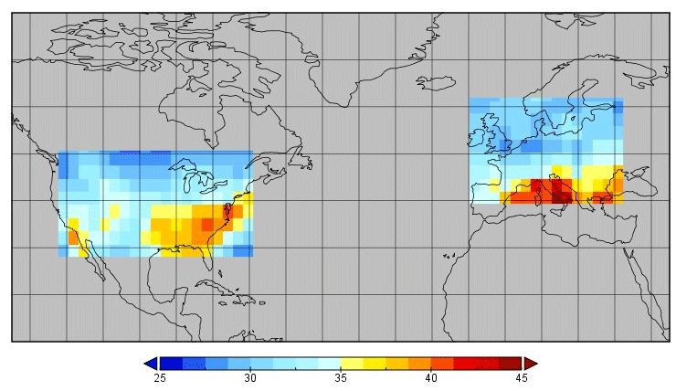
Figure 1 Annual mean surface ozone mixing ratio (in ppb) from the FRSGC/UCI CTM showing the regions considered here and the 272 grid cells used for model calibration.

2.2 Surface O₃ and CO data

Ground-based observations of O₃ are relatively abundant in Europe and North America, where there are ∼ 1800 individual sites that have continuous long-term measurements of O₃ (Chang et al., 2017; Schultz et al., 2017). Measurements of CO are made at fewer locations, but reliable long-term data are available from 57 sites that are part of the Global Atmospheric Watch network (Schultz et al., 2015). To allow more thorough testing of the effects of spatial coverage over these regions, we use Copernicus Atmosphere Monitoring Service (CAMS) interim reanalysis data of surface O₃ and CO from the European Centre for Medium-Range Weather Forecasts (ECMWF) which has been tuned to match measurements using 4D-Var data assimilation (Flemming et al., 2017). This reanalysis reproduces observed O₃ and CO distributions relatively well, and biases at surface measurement stations are generally small (Huijnen et al., 2020). The dataset also has the benefit of complete global coverage, allowing us to test the importance of measurement coverage directly.

Reanalysis data for O₃ and CO are available for 2003–2015, and we average the data by month across this period to provide a climatological comparison. The control run of the FRSGC/UCI model matches CO from the reanalysis data reasonably well (Fig. 2), but overestimates surface O₃. Overestimation of O₃ in continental regions has been noted in previous studies and is partly a consequence of rapid photochemical formation from fresh emissions that are magnified at coarse model resolution (Wild and Prather, 2006). For this exploratory study, we bias-correct the modelled surface O₃ by reducing it by 25 %, following the approach taken by Shindell et al. (2018), so that it matches the reanalysis data (Fig. 2a). This adjustment accounts for the effect of chemical processes and model resolution, which are not explored in this study, and provides a firmer foundation for investigating the effects of other processes.

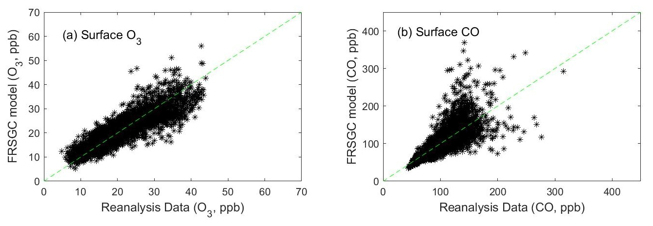
Figure 2 Monthly-mean surface O₃ (a) and surface CO (b) over Europe and North America simulated with the FRSGC/UCI CTM compared with ECMWF reanalysis data.

2.3 Representation error

The “representation error” describes how well measurements made at a single location represent a wider region at the spatial scale of the model ($\mathrm{2.8}{}^{\circ }\times \mathrm{2.8}{}^{\circ }$ for this study). The error may be reduced by averaging measurements made at different stations within a model grid box, although atmospheric measurements may be too sparse to permit this (Lyapina et al., 2016). The representation error is sometimes taken as the mean of the spatial standard deviation of different measurements within a grid box (Sofen et al., 2016). However, this measure quantifies the spatial variability of measured O₃ within a grid box and may not match the representation error.

To test the effect of varying this representation error on parameter estimates, we use synthetic data from the control run of the model using parameters set to their nominal default values. Synthetic O₃ and CO data were generated by adding different levels of representation error for each level of spatial coverage. In mathematical terms, we write the following:

$$\begin{array}{}\text{(1)}& {\text{data}}_i=m_i\left({\mathit{x}}_{\text{control}}\right)+{\mathit{\epsilon }}_i,{\mathit{\epsilon }}_i\sim N(\mathrm{0},{\mathit{\sigma }}_i^{\mathrm{2}}),\end{array}$$

where, for the ith point in space or time, data_i refers to the synthetic data for O₃ or CO, m_i(x_control) is the O₃ or CO from the model control run, and ε_i is generated from a Normal distribution with mean of zero and standard deviation σ_i that is directly proportional to the magnitude of m_i(x_control). In this case, ${\mathit{\sigma }}_i=p\times m_i\left({\mathit{x}}_{\text{control}}\right)$, where p is a scaling factor that provides a measure of the representation error. We used the reanalysis data to estimate p alongside the model parameters, and we found posterior values of p that were in the range 0.16–0.19. We therefore selected four values of p (0.01, 0.1, 0.2 and 0.3) to explore the importance of representation error when using the synthetic data.

2.4 Global sensitivity analysis

Sensitivity analysis was carried out to determine the sensitivity of the simulated surface O₃ and CO to changes in each of the eight parameters. This allows us to identify which of the parameters are most important in governing surface O₃ and CO. We use global sensitivity analysis (GSA), varying each input while averaging over the other inputs. This provides a more integrated assessment of uncertainty than the traditional one-at-a-time approach varying each input in turn while fixing the other inputs at nominal values. We use the extended FAST method (Saltelli et al., 1999), a common and robust approach to GSA in which the sensitivity indices are quantified by partitioning the total variance in the model output (i.e. modelled surface O₃ or CO) into different sources of contribution from each input. Like most sensitivity analysis methods, this approach requires several thousand executions of the model, which would be computationally expensive for the CTM used here. This is overcome by replacing the CTM with a Gaussian process (GP) emulator. Further details of the implementation of GSA are described in Ryan et al. (2018).

2.5 Gaussian process emulation – theory

We replace the CTM with a surrogate model that maps the inputs of the CTM (the eight parameters listed in Table 1) with its outputs (surface O₃ and CO). We employ a surrogate model based on Gaussian process (GP) emulation for three reasons. Firstly, due to the attractive mathematical properties of a GP, the emulator needs very few runs of the computationally expensive model to train it, typically less than 100. This is in contrast to methods based on neural networks, which often have a large number of parameters that necessitate thousands of training runs. Secondly, a GP emulator is an interpolator and so predicts the output of the model with no uncertainty at the input points it is trained at. Thirdly, it gives a complete probability distribution, as a measure of uncertainty, for estimates of the model output at points it is not trained at.

A GP is an extension of the multivariate Gaussian distribution, where instead of a mean vector μ and covariance matrix Σ, mean and covariance functions given by E(f(x)) and $\mathrm{cov}\left(f\left(\mathit{x}\right),f\left({\mathit{x}}^{\prime }\right)\right)$ are used (Rasmussen, 2006). Here, $f\left(\cdot \right):\mathit{\chi }\in {\mathbb{R}}^q\to {\mathbb{R}}^{q^{\prime }}$ represents the computationally expensive model, and χ denotes the input space given by $\mathit{x}=\left(x_{\mathrm{1}},\mathrm{\dots },x_q\right)\in {\mathit{\chi }}_{\mathrm{1}}\times \mathrm{\dots }\times {\mathit{\chi }}_q=\mathit{\chi }\subset {\mathbb{R}}^q$, and q is the number of input variables. GP emulators within a Bayesian framework were first developed in the 1990s and early 2000s (O'Hagan, 2006; Oakley and O'Hagan, 2004; Kennedy and O'Hagan, 2000; Currin et al., 1991). The simplest and most common GP emulator is one where the outputs to be emulated are scalar. Thus, if the computationally expensive model is given by f(⋅), then the one-dimensional output y is calculated by y=f(x). This means that if the model output is multi-dimensional – e.g. a global map or a time series – then we need to build a separate emulator for each point in the output space. Building the emulator requires training runs from the expensive model. In general, we choose n training inputs, denoted by ${\mathit{x}}_{\mathrm{1}},{\mathit{x}}_{\mathrm{2}},\mathrm{\dots },{\mathit{x}}_n$, based on a space-filling design such as a maximin Latin hypercube design (Morris and Mitchell, 1995). The number of training points is based on the rule of thumb $n=\mathrm{10}\times q$ (Loeppky et al., 2012).

Denoting the scalar outputs by y₁=f(x₁), y₂=f(x₂), …, y_n=f(x_n), we then build an emulator $\widehat{f}\left(\cdot \right)$ given by $\widehat{y}=\widehat{f}\left(\mathit{x}\right)$, where $\widehat{y}$ is the estimated output from the emulator. If x represents one of the training inputs (i.e. $\mathit{x}={\mathit{x}}_i,\mathrm{1}\le i\le n)$, then $\widehat{y}$ is equal to the output from f(⋅) with no uncertainty (i.e. $\widehat{y}=y$). If x represents an input the emulator is not trained at, then $\widehat{y}$ has a probability distribution represented by a mean function m(x) and a covariance function $V(\mathit{x},{\mathit{x}}^{\prime })$, where x^′ is a different input. The mean function is given by the following:

$$\begin{array}{}\text{(2)}& m\left(\mathit{x}\right)=h(\mathit{x}{)}^{\mathrm{T}}\widehat{\mathit{\beta }}+t(\mathit{x}{)}^{\mathrm{T}}{\mathbf{A}}^{-\mathrm{1}}\left(\mathit{y}-\mathbf{H}\widehat{\mathit{\beta }}\right),\end{array}$$

where h(x)^T is a $\mathrm{1}\times (q+\mathrm{1}$) vector given by (1,x^T); $\widehat{\mathit{\beta }}$ is a vector of coefficients determined by $\widehat{\mathit{\beta }}={\left({\mathbf{H}}^{\mathrm{T}}{\mathbf{A}}^{-\mathrm{1}}\mathbf{H}\right)}^{-\mathrm{1}}{\mathbf{H}}^{\mathrm{T}}{\mathbf{A}}^{-\mathrm{1}}\mathit{y}$; $t{\left(\mathit{x}\right)}^{\mathrm{T}}=\left(C\left(\mathit{x},{\mathit{x}}_{\mathrm{1}};\mathit{\psi }\right),\mathrm{\dots },C\left(\mathit{x},{\mathit{x}}_n;\mathit{\psi }\right)\right)$; and A is a matrix whose elements are determined by ${\mathbf{A}}_{i,j}=C\left({\mathit{x}}_i,{\mathit{x}}_j;\mathit{\psi }\right)$, $y={\left[f\left({\mathit{x}}_{\mathrm{1}}\right),\mathrm{\dots },f\left({\mathit{x}}_n\right)\right]}^{\mathrm{T}}$, and $\mathbf{H}={\left[h\left({\mathit{x}}_{\mathrm{1}}\right)\mathrm{\dots },h\left({\mathit{x}}_n\right)\right]}^{\mathrm{T}}$. Here, $C\left(\mathit{x},{\mathit{x}}^{\prime };\mathit{\psi }\right)$ is a correlation function that represents our prior belief about how the inputs x and x^′ are correlated. A common choice is a Gaussian correlation function which takes the form: $C\left(\mathit{x},{\mathit{x}}^{\prime };\mathit{\psi }\right)=\exp \left(-{\left(\mathit{x}-{\mathit{x}}^{\prime }\right)}^{\mathrm{T}}\mathbf{B}\left(\mathit{x}-{\mathit{x}}^{\prime }\right)\right)$, where B is a p×p matrix with zeros in the off-diagonals and diagonal elements given by the roughness parameters $\mathit{\psi }=({\mathit{\psi }}_{\mathrm{1}},\mathrm{\dots },{\mathit{\psi }}_q)$. The roughness parameters give an indication of whether the input–output relationship for each input variable, given the training data, should be linear. Low values reflect a linear (or smooth) relationship, whereas high values (e.g. > 20) suggest a non-linear (or non-smooth) response surface. For implementation purposes, we express the correlation function as the following:

$$C\left(\mathit{x},{\mathit{x}}^{\prime };\mathit{\psi }\right)=\sum _{j=\mathrm{1}}^{q+\mathrm{1}}\exp \left(-{\mathit{\psi }}_j{\left({\mathit{x}}_j-{\mathit{x}}_j^{\prime }\right)}^{\mathrm{2}}\right),$$

where $\mathit{x}=(x_{\mathrm{1}},\mathrm{\dots },x_q)$ and ${\mathit{x}}^{\prime }=(x_{\mathrm{1}}^{\prime },\mathrm{\dots },x_q^{\prime })$. The formula for the covariance function $V\left(\mathit{x},{\mathit{x}}^{\prime }\right)$ is given in Appendix A.

A final issue to resolve is how to estimate the roughness parameter since the posterior distribution of f(⋅) is conditional on these emulator parameters. A Bayesian approach would be to integrate out these emulator parameters in the formulation of the GP emulator. This would require highly informative priors, but in most cases such informative priors do not exist. Kennedy and O'Hagan (2001) propose using maximum likelihood to provide a point estimate of the emulator parameters and to use these in the formulae for the mean and covariance functions of the GP emulator. We adopt this approach in this study.

2.6 Gaussian process emulation – implementation

Using the Loeppky rule, we choose n=80 different training inputs for our eight-parameter calibration study. In total, we emulate two variables (surface O₃ and CO) over 12 months at 272 spatial locations, and so we require 6528 different GP emulators. To estimate the model parameters, we evaluate each of the GP emulators tens of thousands of times. Although emulation is computationally fast, this presents a substantial computational burden, even for more computationally efficient versions of the emulator (Marrel et al., 2011; Roustant et al., 2012). We overcome this by computing parts of Eq. (2) prior to these evaluations. Specifically, we compute the vectors $\widehat{\mathit{\beta }}$, m_LP and ψ for all points in the output space, where m_LP denotes ${\mathbf{A}}^{-\mathrm{1}}\left(\mathit{y}-\mathbf{H}\widehat{\mathit{\beta }}\right)$, the last part of m(x) from Eq. (2). We store these three objects as three matrices ${\widehat{\mathit{\beta }}}_{\text{ALL}}$, m_LP.ALL and ψ_ALL. Evaluated at a new input x_new, the mean function of the emulator (Eq. 1) can now be expressed as the following:

$$\begin{array}{}\text{(3)}& \begin{array}{rl}{m}_i\left({\mathit{x}}_{\text{new}}\right)=& h{\left({\mathit{x}}_{\text{new}}\right)}^{\mathrm{T}}{\widehat{\mathit{\beta }}}_{\text{ALL}}\left[i,:\right]+t_i{\left({\mathit{x}}_{\text{new}}\right)}^{\mathrm{T}}{\mathbf{m}}_{\text{LP.ALL}}\left[i,:\right];\\ t_i{\left({\mathit{x}}_{\text{new}}\right)}^{\mathrm{T}}=& \left(C\left({\mathit{x}}_{\text{new}},x_{\mathrm{1}};{\mathit{\psi }}_{\text{ALL}}[i,:]\right),\mathrm{\dots },\right.\\ & \left.C\left({\mathit{x}}_{\text{new}},x_n;{\mathit{\psi }}_{\text{ALL}}[i,:]\right)\right);\end{array}\end{array}$$

where i ($\mathrm{1}\le i\le \mathrm{6528}$) denotes the ith point in the output space, and $[i,:]$ refers to the ith row of each matrix. The equivalent formula for $V\left(\mathit{x},{\mathit{x}}^{\prime }\right)$ is given in Appendix A.

To test the accuracy of GP emulation, we ran each of the 6528 emulators at 20 sets of parameters which were not used for training the emulators. The estimated O₃ and CO values from the emulators for all spatial locations and months closely match the simulated O₃ and CO output from the FRSGC/UCI model for these validation runs, with R²>0.995 for each variable; see Fig. 3.

Finally, we recognise that principal component analysis (PCA) could be used to reduce the dimensionality of the output space and hence the number of emulators required (Higdon et al., 2008). In a previous study we found that a PCA–emulator hybrid approach resulted in similar performance compared to using separate emulators for each point in the output space, and this reduced the number of emulators required from 2000 to 40 or fewer (Ryan et al., 2018). However, for this study, we choose an emulator-only approach, because it is much simpler to demonstrate. Nonetheless, future emulation–calibration studies could benefit from the computational savings of applying a PCA–emulator hybrid approach. Other approaches for dealing with high-dimensional output are also available, such as low rank approximations (Bayerri et al., 2007).

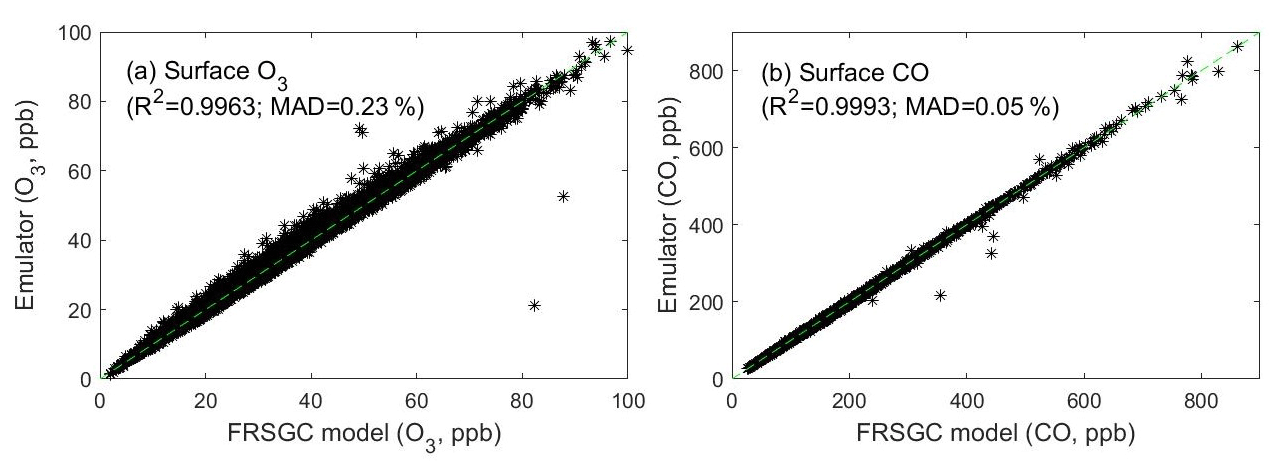
Figure 3 Simulated surface O₃ (a) and surface CO (b) from the FRSGC/UCI CTM versus those predicted from the Gaussian process emulators. The simulated and emulated concentrations were generated using 20 sets of model parameters that were not used for training the emulators.

2.7 Parameter estimation

We estimate the eight model parameters using Bayesian statistics via the software package Just Another Gibbs Sampler (Plummer, 2003). This uses Gibbs sampling, which is an approach based on Markov Chain Monte Carlo (MCMC) that we use to determine the multi-dimensional posterior probability distribution of the model parameters (Gelman et al., 2013). Gibbs sampling is an extension of the more traditional Metropolis–Hastings variant of MCMC, and uses conditional probability to sample from the marginal distribution when moving around the multi-dimensional parameter space.

To find the posterior distribution, the MCMC algorithm searches the parameter space using multiple sets of independent chains. Here, a chain refers to a sequence of steps in the parameter space that the algorithm takes. A new proposed parameter set in this search is accepted on two conditions: (1) the set is consistent with the prior probability distribution, which for our study was a set of uniform distributions with the lower and upper bounds given by the defined ranges in Table 1; and (2) the resulting modelled values using the proposed set of parameters are consistent with measurements, which is assessed using the following Gaussian likelihood function:

$$\begin{array}{}\text{(4)}& L\left(\mathit{\theta }\right)=\prod _{i=\mathrm{1}}^N{\displaystyle \frac{\mathrm{1}}{\sqrt{\mathrm{2}\mathit{\pi }{\mathit{\sigma }}_i}}}\exp {\left({\displaystyle \frac{f_i\left(\mathit{\theta }\right)-m_i}{{\mathit{\sigma }}_i^{\mathrm{2}}}}\right)}^{\mathrm{2}},\end{array}$$

where N is the number of measurements used, f_i(θ) is the ith model output ($\mathrm{1}\le i\le N$) using the proposed parameter set θ, m_i is the measurement corresponding to the ith model output and σ_i is the representation error for measurement m_i. We note that although separate emulators are used for each of the spatial and temporal locations in the model output, there is still only a single likelihood function. Hence, evaluating all of the emulators for a specific set of values of the scaling parameters is equivalent to evaluating the CTM once at those values of the parameters.

We ran three parallel chains for 10 000 iterations each. After discarding the first half of these iterations as “burn in”, we thinned the chains by a factor of 5 to reduce within-chain autocorrelation. Convergence was assessed using the Brooks–Gelman–Rubin diagnostic tool (Gelman et al., 2013). This produced 3000 independent samples from the posterior distribution for each parameter, which we summarise using their posterior means and 95 % credible intervals (CIs) defined by the 2.5th and 97.5th percentiles (Gelman et al., 2013). We used the R language to code up our configuration of the MCMC algorithm.

2.8 Model discrepancy

It has been suggested that a model discrepancy term should be included when carrying out model calibration involving Gaussian process emulators (e.g. Kennedy and O'Hagan, 2001; Brynjarsdóttir and O'Hagan, 2014). The discrepancy term represents the processes missing in the model. However, in this demonstration study we have chosen not to include a discrepancy term for two reasons. Firstly, for scenarios where we use synthetic data, no discrepancy term is required, because the synthetic data are generated by adding noise and spatial gaps to the emulator output for the control run. Secondly, for scenarios involving reanalysis data, there is no simple and defensible method to estimate the term. When performing model calibration by applying MCMC directly, a discrepancy term would not be included. Since the purpose of the emulator here is to estimate the output of the model for a given set of parameter values, we argue that it is not necessary to include a discrepancy term into the calibration formulation. However, we agree that including such a term may be helpful in situations where there is good prior information.

To investigate the importance of a discrepancy term, we repeat the experiment to estimate the eight scaling parameters using surface ozone reanalysis data and assuming a discrepancy term that is 10 % of the magnitude of the observation. We find that there is almost no difference in the marginal posterior distribution when we include the discrepancy term compared with when we omit it (see Fig. S16 in the Supplement). We therefore choose to omit the term for our study.

2.9 Experimental approach

We first perform a global sensitivity analysis to identify the parameters which have the greatest influence on the two variables we consider. We then perform parameter estimation using surface concentration data over the regions of North America and Europe shown in Fig. 1 and focus our analysis on the parameters which have the greatest influence. To provide a demonstration of the approach, we first use “synthetic” measurement data drawn from the control run of the CTM which were not used to train the emulators, adding increasing levels of noise to represent measurement representation errors of 1 %, 10 %, 20 % and 30 % (p=0.01, 0.1, 0.2 and 0.3), and varying the spatial coverage of these measurements over the regions considered over a wide range: 2.5 %, 5 %, 10 %, 20 %, 40 % and 100 %. We focus on surface O₃ only, surface CO only and then both variables together. We then use the reanalysis data to represent the measurements, focussing on the effects of spatial coverage alone and estimating the representation error p from this independent dataset. The 90 different scenarios we consider are summarised in Table 2. We discuss the implication of these results and the limitations of considering a simple eight-parameter system rather than all sources of model uncertainty in Sect. 4.

Table 2 Summary of the 90 different MCMC scenarios carried out for this study. The scenarios involved varying (i) the type of data (synthetic or reanalysis); (ii) the representation error used for the synthetic data (p), where m_i(x_control) is the control run output of the CTM, and σ_i is the amount of statistical noise added; (iii) the percentage coverage of grid squares in the USA and Europe. For the synthetic data, the 24 scenarios correspond to a full factorial combination of four levels of representation error and six levels of spatial coverage, while for the reanalysis data the six scenarios correspond to the six levels of spatial coverage.

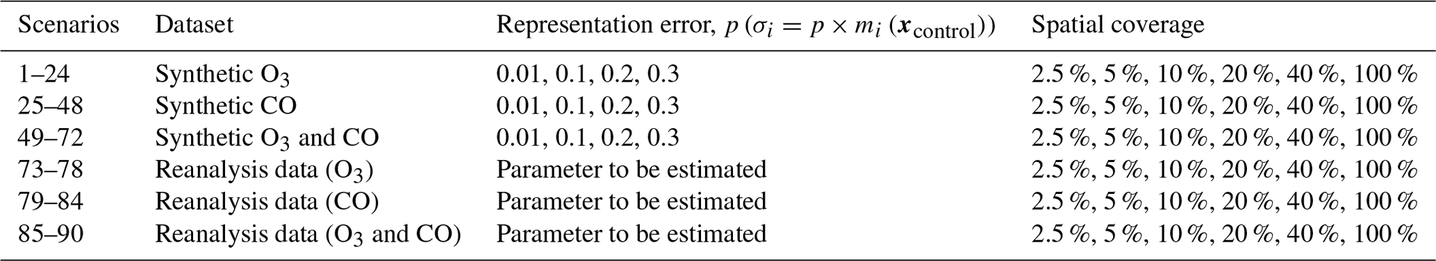
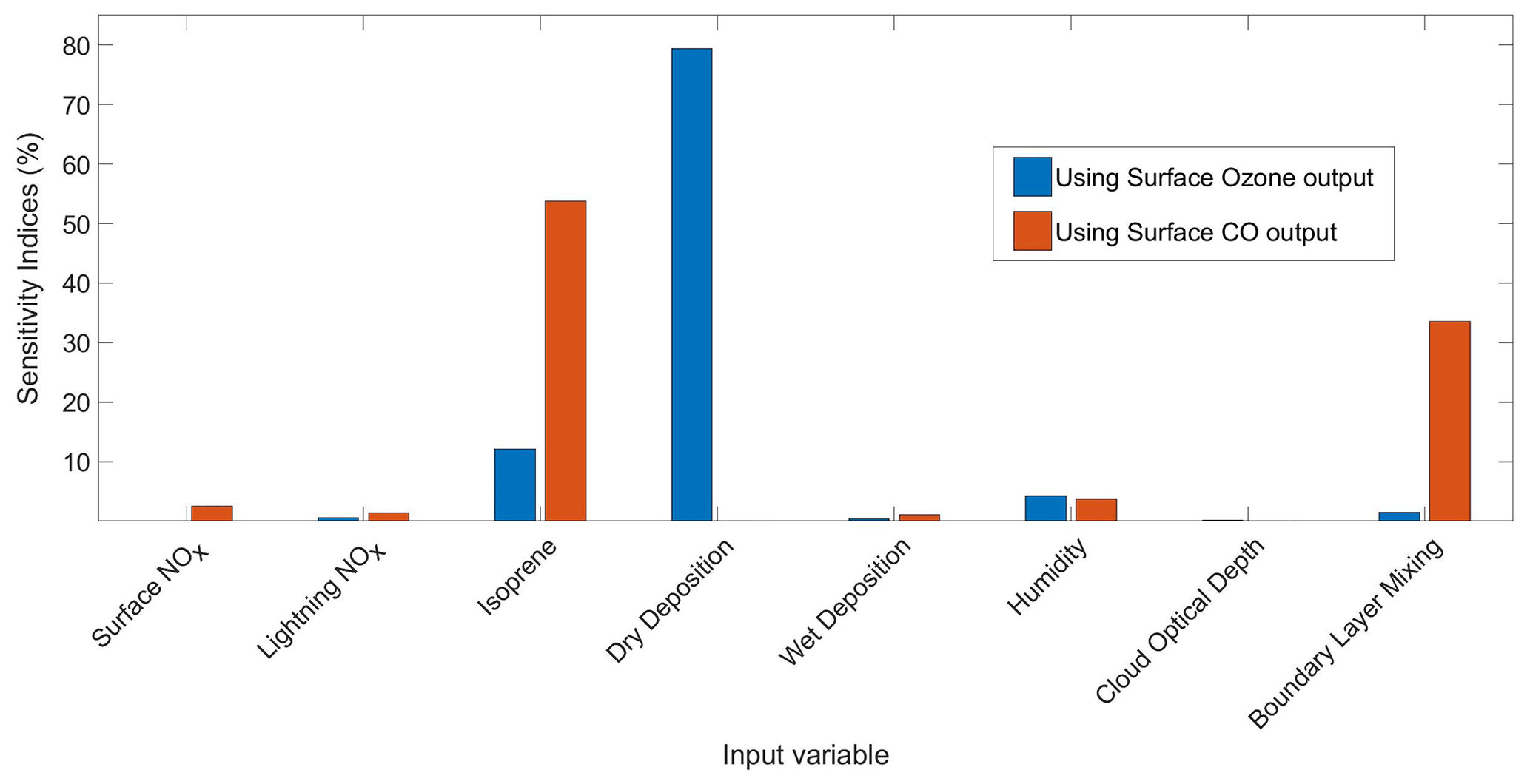
Figure 4 Sensitivity indices representing the percentage of the variance in surface O₃ and CO over the USA and Europe in the FRSGC/UCI model output due to changes in the scaling parameter associated with each of the eight model processes (Table 1).

3 Results

3.1 Global sensitivity analysis

Results from global sensitivity analysis reveal that over the continental regions of Europe and North America considered here the simulated monthly-mean concentrations of surface O₃ are most sensitive to dry deposition and, to a lesser extent, to isoprene emissions (Fig. 4). This is not unexpected, given the importance of direct deposition of ozone to the Earth's surface, and the role of isoprene as a natural source of ozone in continental regions. The simulated surface CO is most sensitive to isoprene emissions, which represent a source of CO, and to boundary layer mixing, which influences the transport of CO from polluted emission regions. We thus identify the scaling parameters corresponding to dry deposition, isoprene emissions and boundary layer mixing as the most important of the eight considered here to estimate accurately to reduce the bias in modelled surface O₃ and CO. For completeness, we show the geographical distribution of sensitivity indices in Figs. 5 and 6, which reveal the importance of humidity in governing O₃ over oceanic regions and highlight the very different responses of surface O₃ and CO to the major driving processes.

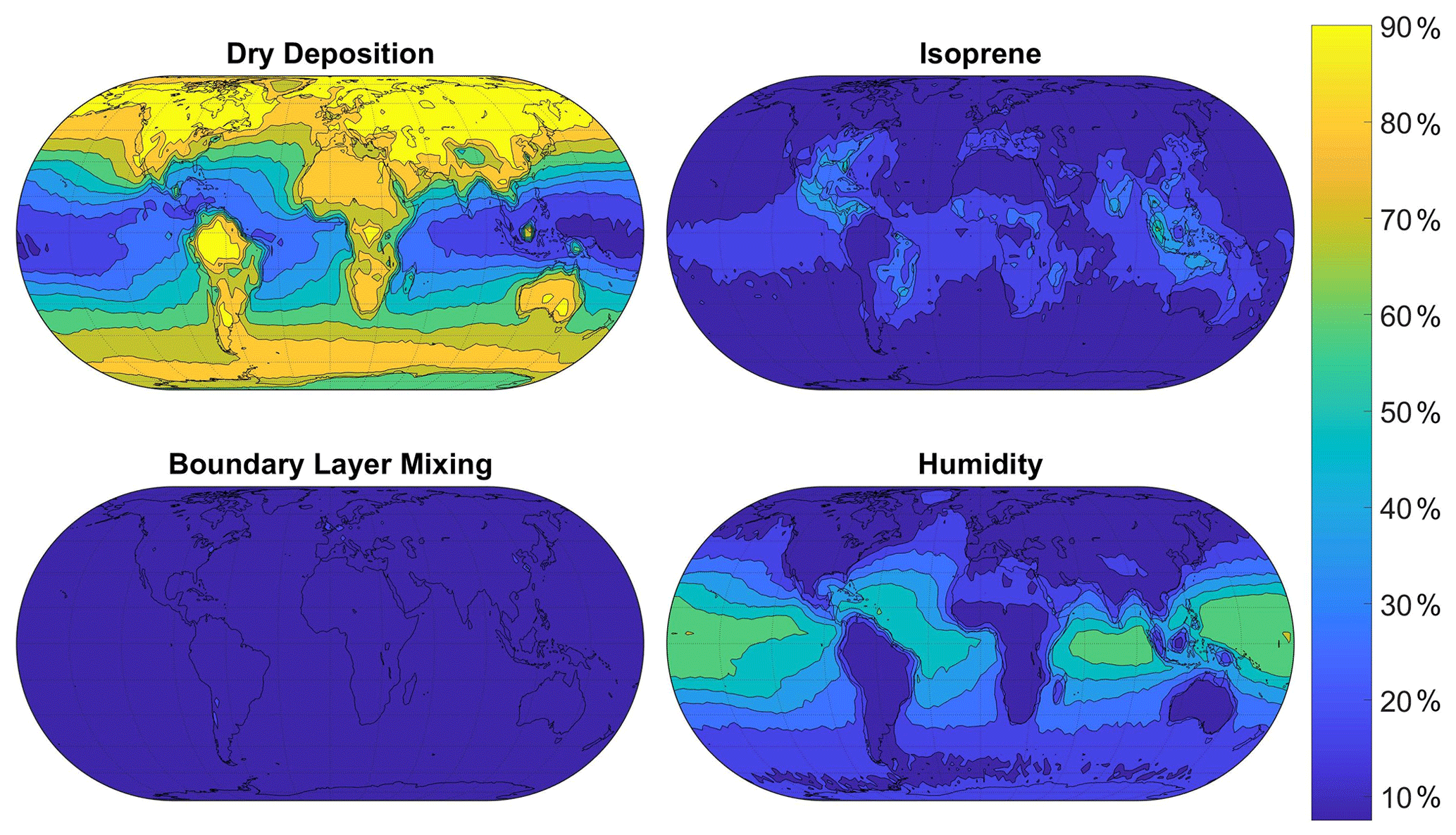
Figure 5 Sensitivity indices representing the percentage of the variance in surface O₃ in the FRSGC/UCI model output due to changes in each input parameter. The four parameters displayed here have the highest sensitivity indices and the largest effect on simulated surface O₃. Maps of sensitivity indices corresponding to the other four parameters are shown in Fig. S2 of the Supplement.

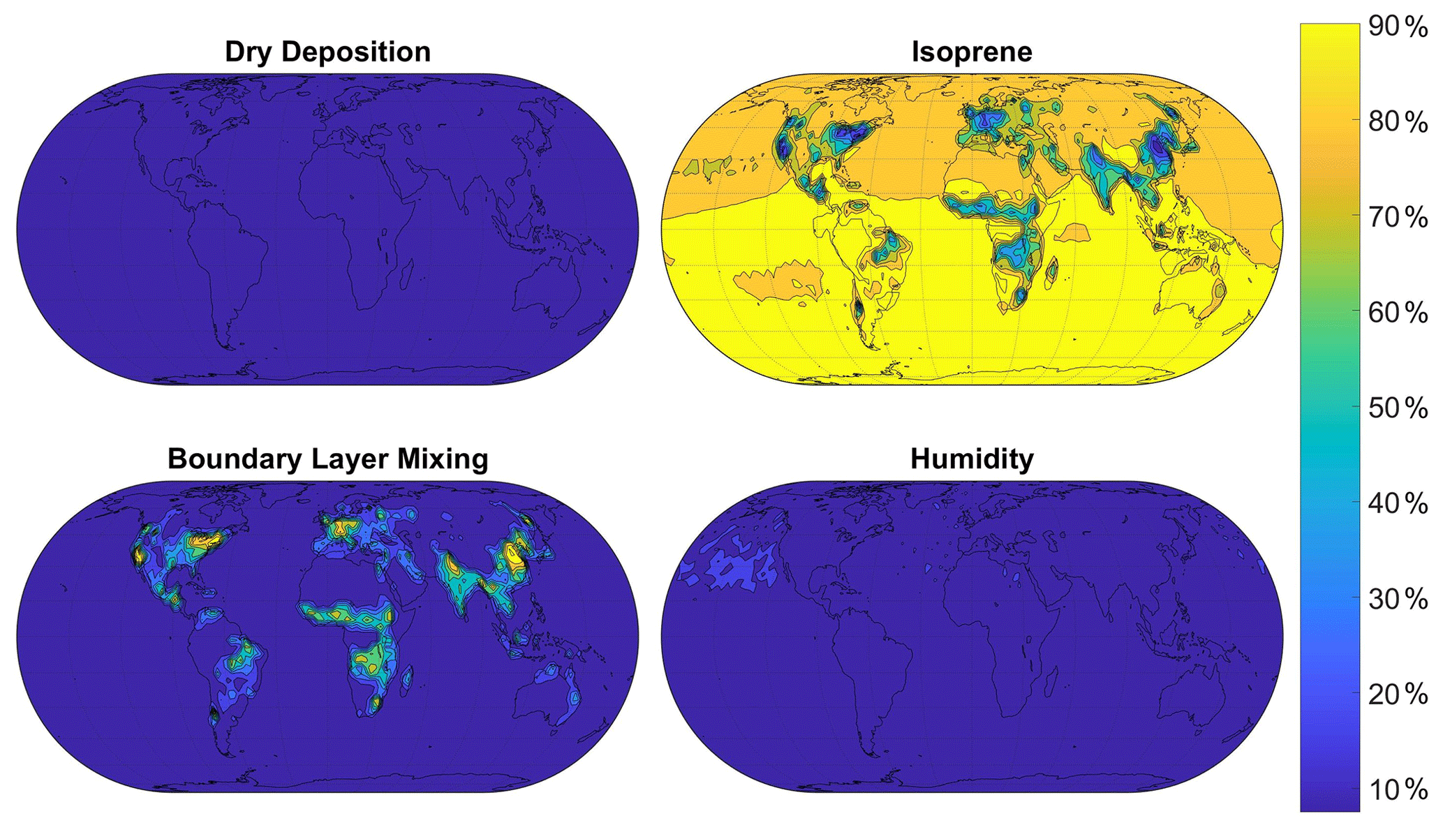
Figure 6 Sensitivity indices representing the percentage of the variance in surface CO in the FRSGC/UCI model output due to changes in each input parameter. Maps of sensitivity indices for the other four parameters are shown in Fig. S3 of the Supplement.

3.2 Estimation of scaling parameters using synthetic data

We next use synthetic observation data to calibrate the model and estimate scaling parameters. For synthetic data, we use the model control run with a specified level of representation error (Table 2), and the default model parameters define the true scaling that we aim to retrieve. Prescribing surface O₃ with very little error (p=0.01) gives an estimate of the dry deposition scaling parameter, which has the largest influence on modelled surface O₃, close to its true value and the uncertainty is small even when the spatial coverage of measurements is only 2.5 % (Fig. 7, column 1). As the representation error is increased to p=0.1, the parameter uncertainty is larger at low spatial coverage, but the mean estimate remains unbiased (Fig. 7, column 2). The uncertainty at all levels of spatial coverage becomes larger as p increases to 0.2 and 0.3, but the means remain very close to the true values (Fig. 7, columns 3 and 4). Surface CO is largely unaffected by dry deposition and thus provides very little constraint on the scaling parameter. The effect of prescribing surface CO and O₃ together is very similar to that of using surface O₃ alone.

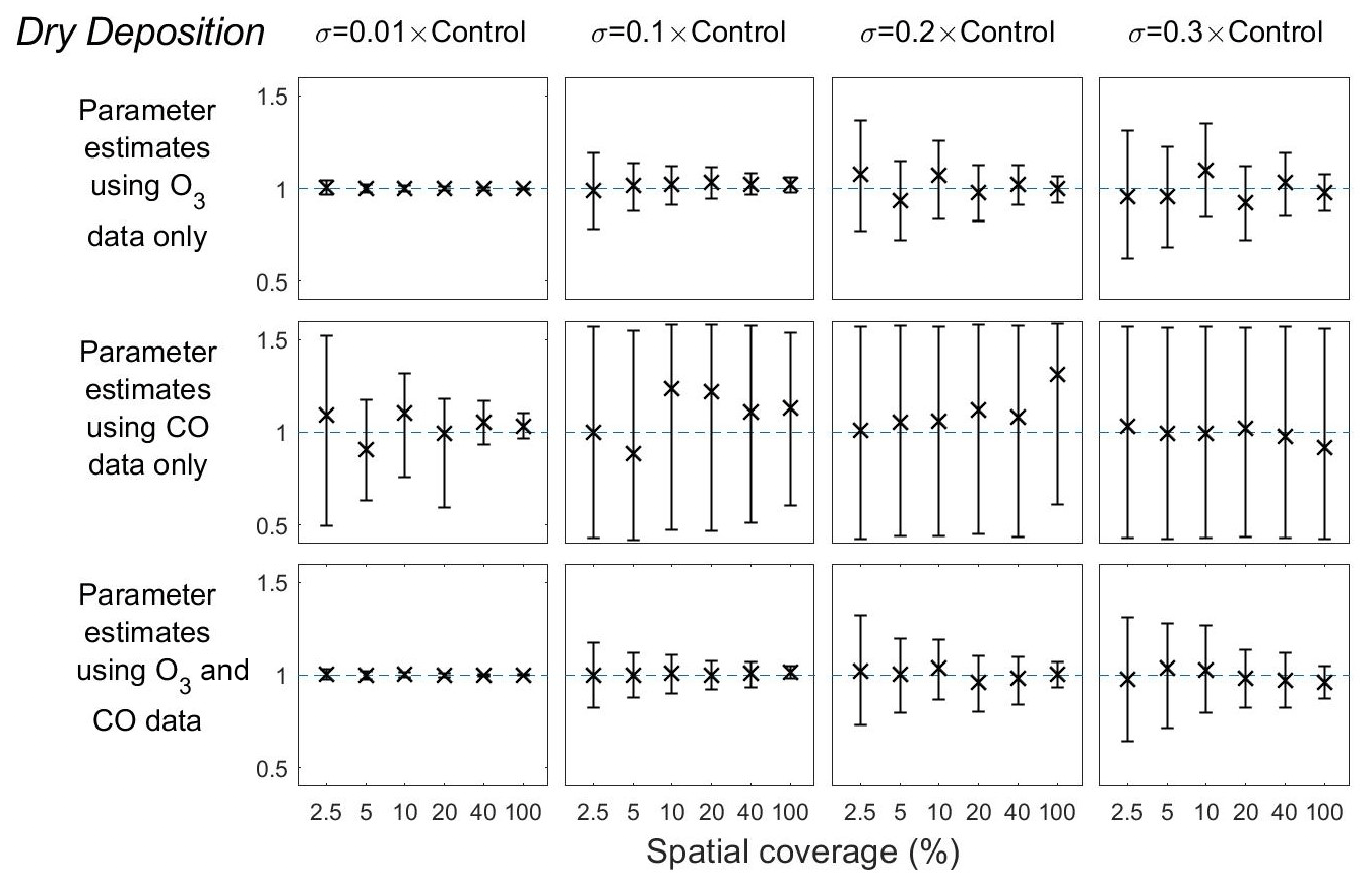
Figure 7 Means and 95 % credible intervals of 3000 samples of the dry deposition scaling parameter from posterior distributions using the MCMC algorithm based on synthetic datasets from scenarios 1–72 (Table 1). Control refers to the FRSGC/UCI model control run surface concentration for each output point.

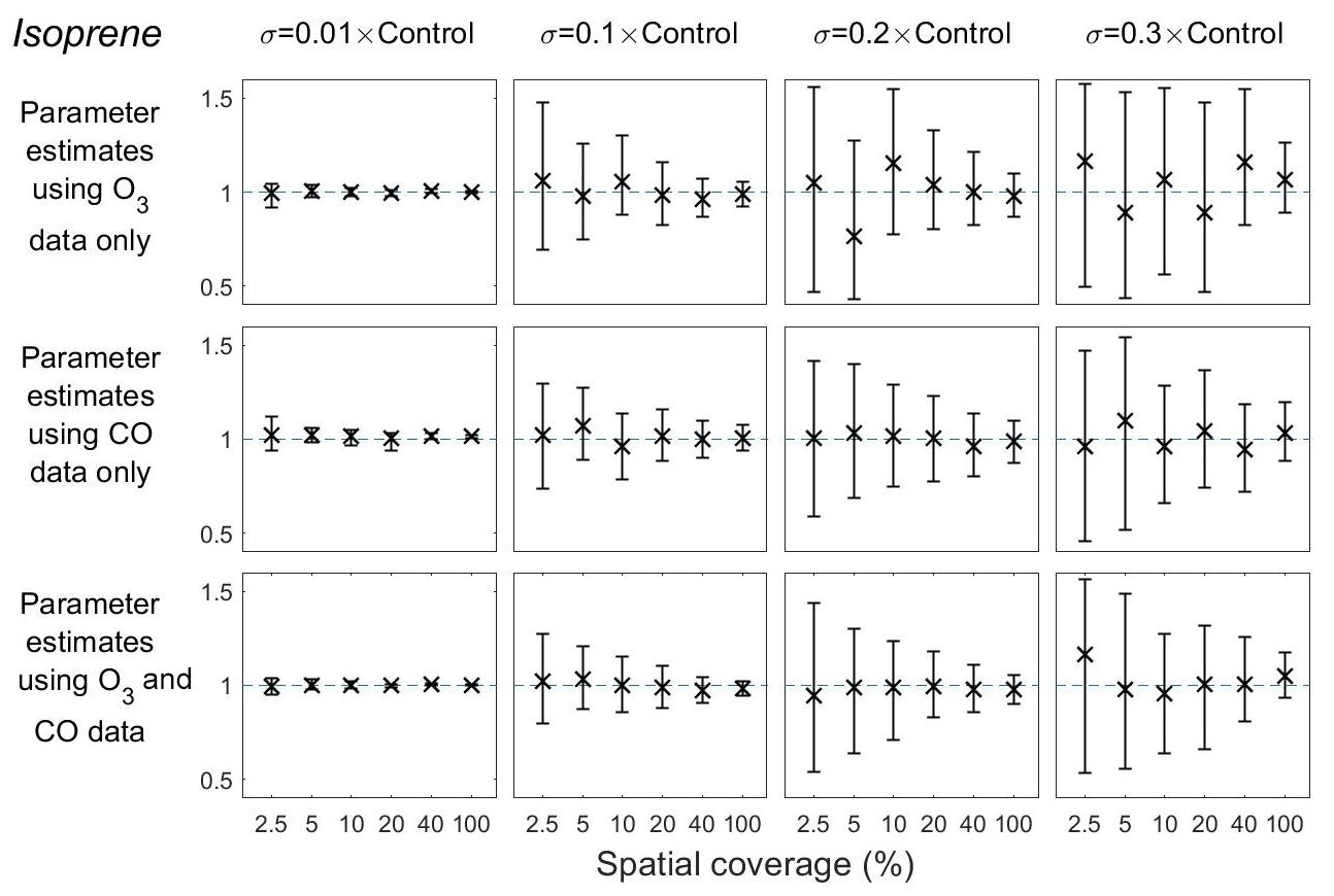
Figure 8 Means and 95 % credible intervals of 3000 samples of the isoprene emission scaling parameter from posterior distributions using the MCMC algorithm based on synthetic datasets from scenarios 1–72 (Table 1). Control refers to the FRSGC/UCI model control run surface concentration for each output point.

Using surface CO alone with very little representation error (p=0.01), the mean estimate of the isoprene emission scaling parameter is equal to the true value with very little uncertainty, regardless of the spatial coverage (Fig. 8, column 1). When the representation error is increased to p=0.1, the estimate remains very close to the true value, but the uncertainty is substantially higher at low spatial coverage (2.5 % and 5 %) than at higher coverage (40 % and 100 %) (Fig. 8, column 2). The estimates deviate further from the truth at higher levels of representation error (p=0.2 and 0.3) and the uncertainty is greater (Fig. 8, columns 3 and 4). Estimates of the isoprene scaling parameter are less accurate than those of the dry deposition scaling parameter, as the posterior means are further from the true value of the parameter, and the uncertainty intervals are wider (Fig. 8 vs. Fig. 7). As with our findings for dry deposition, the posterior means and the lengths of the uncertainty intervals for the isoprene scaling parameter remain relatively unchanged when surface O₃ data are prescribed at the same time.

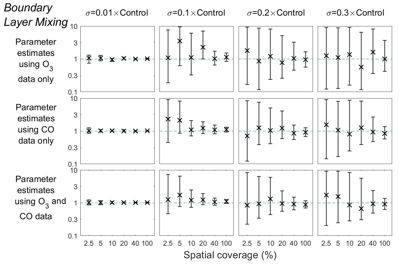
Figure 9 Means and 95 % credible intervals of 3000 samples of the Boundary layer mixing scaling parameter from posterior distributions using the MCMC algorithm based on synthetic datasets from scenarios 1–72 (Table 1). Control refers to the FRSGC/UCI model control run surface concentration at each output point. The scaling parameter values are given here on a log₁₀ scale.

Our findings for the boundary layer mixing scaling parameter follow a similar pattern to the other two parameters (Fig. 9). In all combinations of representation error and spatial coverage, we find that the mean estimates are unbiased. Furthermore, we find that the parameter uncertainty is significantly smaller when the spatial coverage is 10 % or higher when p=0.1, 20 % or higher when p=0.2, and 40 % or higher when p=0.3 (Fig. 9, Table 2). It is clear from these results that the scalings for these three model parameters can be successfully estimated from synthetic data with low uncertainty when the representation error is low and that the estimates remain good, albeit with higher uncertainty, at higher representation error if the spatial coverage is relatively good.

3.3 Estimation of scaling parameters using reanalysis data

We consider next the CAMS interim reanalysis data for surface O₃ and CO, which are based on assimilated concentrations from the ECMWF model and are thus independent of the FRSGC/UCI model. The reanalysis is representative of similar spatial scales to the FRSGC/UCI model; thus, we ignore the representation error and vary the spatial coverage only. However, we are able to estimate the representation error factor p by treating it as a parameter to estimate. With 100 % spatial coverage, this error term is estimated with the MCMC algorithm to be $p=\mathrm{0.168}\pm \mathrm{0.004}$ and $p=\mathrm{0.191}\pm \mathrm{0.005}$ for surface O₃ and CO, respectively. Although we do not know the true values of the parameters in this case, the good agreement between the control run of the FRSGC/UCI model and the reanalysis data suggests that they lie close to their true values.

Using the reanalysis data for surface O₃ alone, we find that the posterior means and uncertainty for the dry deposition parameter are in the upper half of the range defined, indicating that the real dry deposition flux is greater than that calculated with the FRSGC/UCI model. This is largely as expected, as the FRSGC/UCI model overestimates surface O₃ at these continental sites and greater deposition would bring the model into better agreement with the reanalysis. As the spatial coverage is increased, the estimate of the scaling factor increases to around 1.4, and the uncertainty is reduced (Fig. 10a). In contrast, using surface O₃ and CO together results in an estimate closer to 1 and an additional reduction in uncertainty (Fig. 10g). Inclusion of surface CO measurements, as an additional constraint to surface O₃, results in an estimate of the dry deposition parameter closer to that modelled.

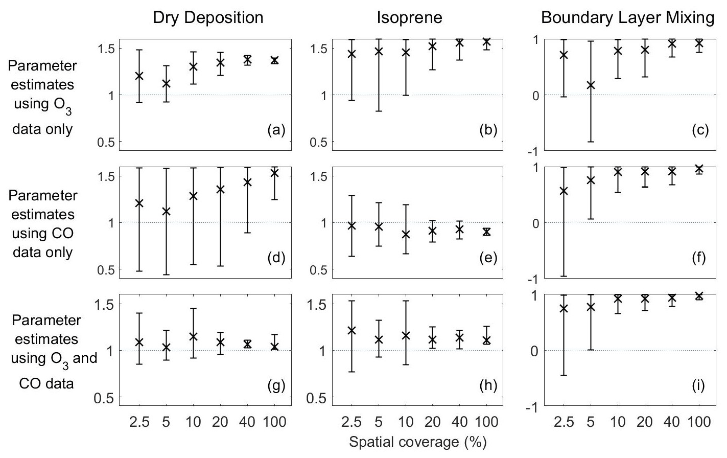
Figure 10 Means and 95 % credible intervals of 3000 samples of the dry deposition, isoprene and boundary layer mixing scaling parameters from posterior distributions using the MCMC algorithm based on reanalysis datasets from scenarios 73–90 (Table 1). The first and second rows show these parameters estimated using one stream of data (O₃ for the first row and CO for the second row), while the third row shows estimates using two data streams (O₃ and CO).

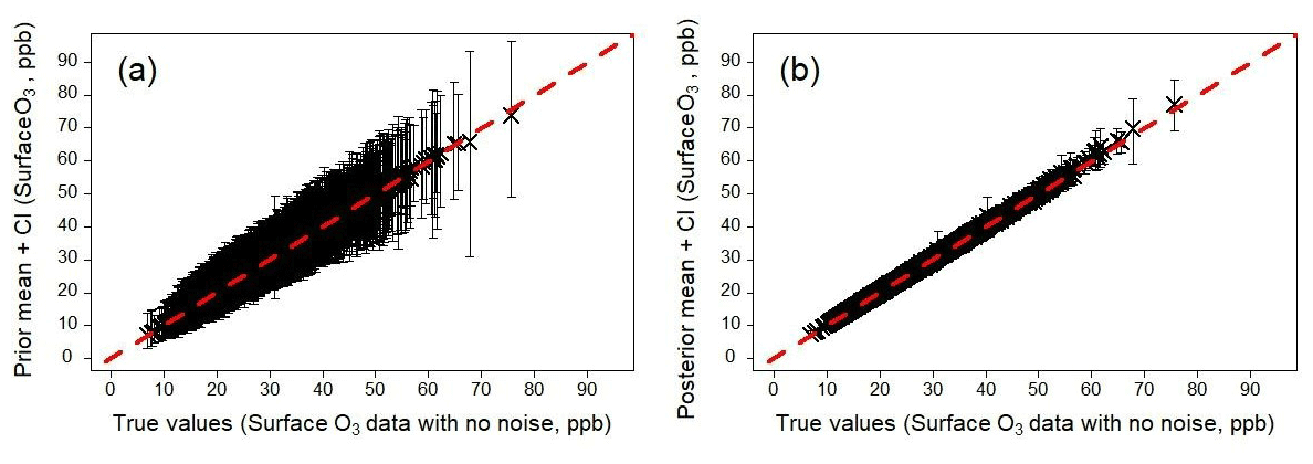
Figure 11 Emulator predictions of surface O₃, evaluated at values of the scaling parameters sampled from the prior distribution (a) and posterior distribution (b), showing the effects of calibration. In panel (b), the outputs correspond to the scenario where the calibration involved synthetic O₃ data, a representation error of p=0.2 and a spatial coverage of 20 % (Table 2). The predictions shown here are carried out for all model grid boxes, i.e. 100 % spatial coverage.

Using surface CO alone, estimates of the isoprene scaling parameter lie in the central part of the defined range, whilst estimates of the boundary layer mixing scaling parameter lie in the upper half of the defined range (Fig. 10e, f). For both parameters, increasing the spatial coverage leads to a reduction in uncertainty. Unlike for dry deposition, inclusion of surface O₃ when estimating either of these parameters results in very little difference in the magnitude of the estimate or in the associated uncertainty (Fig. 10e vs. 10h; Fig. 10f vs. 10i).

3.4 Evaluation of surface O₃ following calibration

We demonstrate the benefit of the calibration by evaluating the emulators using the values of the scaling parameters sampled from the prior and posterior distributions. As an example, we show surface O₃ before and after calibration using the calibration runs involving synthetic data at 20 % spatial coverage and a representation error of p=0.2 (Fig. 11). Despite the calibration involving only 20 % spatial coverage, we apply the resulting parameter values to all grid squares. We can clearly see that the prior surface O₃ concentrations are unbiased but have large uncertainty, especially at high values. In contrast the calibrated O₃ concentrations have a small uncertainty, demonstrating that even with 20 % spatial coverage in the calibration data we are able to achieve improved predictions for all model grid boxes.

4 Discussion

4.1 Representation error

Our results show the impact of the size of the representation error on the accuracy of estimated model parameters. The parametric uncertainty (i.e. the size of the credible intervals in Figs. 7–9) increases at an approximately linear rate as the representation error increases from p=0.01 to p=0.3. This is consistent with Hill et al. (2012), who estimated the parameters and uncertainties of a simple terrestrial carbon model under varying levels of measurement error.

For the reanalysis data, we treat the representation error as a parameter for the MCMC algorithm to estimate along with the eight model parameters. This is possible because we assume that the measured value of O₃ is proportional to the simulated value from a forward run of the FRSGC/UCI model, although such an assumption may not be possible in other situations. An alternative approach to estimate the representation error would be to carry out an intensive measurement campaign to determine whether the average O₃ from different measuring stations within a grid square is representative of the true average. Satellite products of the terrestrial biosphere are checked for accuracy using this type of approach (De Kauwe et al., 2011). Although measurement campaigns at these large spatial and temporal scales would be challenging and costly, they may not need to continue for long periods of time since we might expect representation error to decrease as the temporal scale increases (Schutgens et al., 2016).

4.2 Spatial coverage

We find that as the volume of measurements increase, the estimates of the model parameters are closer to the truth, and the width of the credible intervals decrease. This is particularly clear for the dry deposition and isoprene emission scaling parameters when using both O₃ and CO concentrations (Figs. 8 and 9). While this highlights the value of good spatial coverage, we note that the benefits are greatly reduced if the representation error is relatively high. For the boundary layer mixing parameter, we find little decrease in the credible intervals using synthetic CO data with the highest representation error (p=0.3), where the spatial coverage is less than 20 % (Fig. 9, row 2). In contrast, at the p=0.1 level, a large decrease in uncertainty is seen between the 2.5 % and 20 % coverage. Similar effects are seen, to a lesser extent, for the dry deposition and isoprene scaling parameters as the spatial coverage increases.

Our results using synthetic data show that while the size of the uncertainty intervals varies substantially depending on the spatial coverage or representation error, the posterior means are for the most part very close to the true values. Deviation from these typically occurs when the measurements contain less information either due to low spatial coverage or high representation error. However, the uncertainty intervals include the true values of the parameters for all the experimental scenarios considered here, unlike in Hill et al. (2012). This gives strong confidence in the reliability of the MCMC method used to estimate the parameters.

4.3 Applying multiple constraints

The importance of multiple constraints was most apparent for scenarios involving the reanalysis data. For the dry deposition scaling parameter, which explains much of the variance in surface O₃ (Fig. 4), we found that using O₃ data alone results in mean estimates that are in the upper half of the range of possible values (Fig. 10a). However, including CO data brought the mean estimates into the central part of the range where we would expect the true value to lie (Fig. 10g). This is remarkable given that dry deposition is not an important process for controlling CO, and highlights the coupling between processes that permits constraints on one process from one variable to influence those on another. However, it is consistent with previous studies exploring the uncertainty in estimates of key parameters in an aerosol–chemistry–climate model (Johnson et al., 2018). For the isoprene emission and boundary layer mixing scaling parameters, there was little difference in the mean estimates or the size of the uncertainty intervals when using O₃ and CO together rather than a single constraint. This reveals that the importance of using multiple constraints is dependent on the process and on the variable constrained. A judicious choice of these could allow a particular process to be targeted.

Overall, our estimates of the dry deposition and isoprene emission scaling parameters are close to a priori values from the FRSGC/UCI CTM, with respect to the independent reanalysis data. In contrast, our estimates of the boundary layer mixing scaling parameter are substantially larger than those from the model, suggesting that this process is not represented well in the model or that other processes not considered here may be influencing the result.

4.4 Towards constraint with real surface measurements

Our results have demonstrated the feasibility of using measurement data to constrain model parameters under the right conditions. We have chosen to use synthetic data as they have allowed us to vary the spatial coverage and to investigate the effects of representation error which is poorly characterised when using real measurements data. Quantifying this type of error for real measurements is difficult because measurement sites are relatively sparse and are often representative of a limited area rather than the larger area typical of a model grid square. However, this study has allowed us to estimate the representation error associated with the reanalysis data, and in the absence of more information, these values could be used as a guide when applying surface measurements as a constraint.

The reanalysis data provide a more critical test, as they are independent of the FRSGC/UCI CTM used here. Although we do not know the true values of the scaling parameters, we expect them to lie close to those used in the control run given the relatively good agreement for O₃ and CO concentrations. For the dry deposition parameter, we expect scaling values to be close to 1, but using surface O₃ reanalysis data alone, we found posterior mean scaling parameters approaching 1.4, with credible intervals that did not include 1 (Fig. 10a). This likely reflects overestimation of surface O₃ in continental regions in the CTM and may reflect uncertainties and biases in other processes not considered here, most notably in the chemical formation and destruction of O₃ and in model transport processes. In the absence of consideration of the uncertainty in these processes in this feasibility study, the dry deposition parameter is used as a proxy process to reduce O₃ concentrations. This is an example of equifinality, where different sets of parameters can result in model predictions that give equally good agreement with observations (Beven et al., 2001). Applying simultaneous constraints to CO goes some way to addressing this but does not remove the problem. Before applying real surface measurements to constrain the CTM, we propose a more comprehensive assessment of model uncertainties with a wider range of parameters, so the constraints can more directly inform process understanding and model development.

5 Conclusion

We have demonstrated the use of surface O₃ and CO concentrations to constrain a global atmospheric chemical transport model and generate accurate and robust estimates of model parameters. This would normally be prohibitive for such a model given that thousands of model runs are required. Our approach is to replace the CTM with a surrogate model using Gaussian process emulation and then estimate the parameters using the emulator in place of the CTM. In this feasibility study we have shown that surface O₃ has a large sensitivity to dry deposition and that surface CO is most sensitive to isoprene emissions and boundary layer mixing processes, as expected. We find that estimates of the scaling parameters for these processes are dependent on the spatial coverage and representation error of the surface O₃ and CO data. Our parameter estimates become less uncertain as coverage increases and as the representation error decreases, whilst remaining unbiased. Furthermore, we show that using two separate data constraints, in this case surface O₃ and CO, instead of a single one can result in mean parameter estimates that are much closer to their likely true values. However, this is dependent on the processes considered and constraints applied, and while it is effective for dry deposition here, we find relatively little improvement in the estimates or uncertainties for isoprene emission or boundary layer mixing processes that are also considered here.

The approach we adopt here provides a means of constraining atmospheric models with observations and identifying sources of model error at a process level. Our results based on the independent reanalysis data suggest that dry deposition and isoprene emissions are represented relatively well in the FRSGC/UCI CTM but that boundary layer mixing processes may be somewhat underestimated. However, we have explored the effect of only eight parameters in this study, and consideration of a more complete set of processes, including those governing photochemistry and dynamics, is needed to generate more realistic constraints for key pollutants such as O₃. We aim to expand this study to investigate a more extensive range of parameters and processes and to constrain with a wider range of observation data. The emulator-based approach for estimating parameters that we have successfully demonstrated here can be applied to any model where evaluating the model the required number of times is too computationally demanding.

Appendix A

The formula for the covariance function $V\left(\mathit{x},{\mathit{x}}^{\prime }\right)$ from Sect. 2.2 is given by:

$$\begin{array}{rl}V\left(\mathit{x},{\mathit{x}}^{\prime }\right)=& {\mathit{\sigma }}^{\mathrm{2}}\left[C\left(\mathit{x},{\mathit{x}}^{\prime };\mathit{\psi }\right)-t\left(\mathit{x}{)}^{\mathrm{T}}{\mathbf{A}}^{-\mathrm{1}}t\right(\mathit{x})\right.\\ & +\left(h(\mathit{x}{)}^{\mathrm{T}}+t(\mathit{x}{)}^{\mathrm{T}}{\mathbf{A}}^{-\mathrm{1}}\mathbf{H}\right){\left({\mathbf{H}}^{\mathrm{T}}{\mathbf{A}}^{-\mathrm{1}}\mathbf{H}\right)}^{-\mathrm{1}}\\ & \left.{\left(h({\mathit{x}}^{\prime }{)}^{\mathrm{T}}+t({\mathit{x}}^{\prime }{)}^{\mathrm{T}}{\mathbf{A}}^{-\mathrm{1}}\mathbf{H}\right)}^{\mathrm{T}}\right],\end{array}$$

where

$${\mathit{\sigma }}^{\mathrm{2}}={\displaystyle \frac{{\mathit{y}}^{\mathrm{T}}\left({\mathbf{A}}^{-\mathrm{1}}-{\mathbf{A}}^{-\mathrm{1}}\mathbf{H}{\left({\mathbf{H}}^{\mathrm{T}}{\mathbf{A}}^{-\mathrm{1}}\mathbf{H}\right)}^{-\mathrm{1}}{\mathbf{H}}^{\mathrm{T}}{\mathbf{A}}^{-\mathrm{1}}\right)\mathit{y}}{n-q-\mathrm{1}}}.$$

To compute the variance or uncertainty of a prediction x, we use the formula for $V(\mathit{x},{\mathit{x}}^{\prime })$ with ${\mathit{x}}^{\prime }=\mathit{x}$, which results in $C(\mathit{x},\mathit{x};\mathit{\psi })=\mathrm{1}$. Since we need to evaluate a large number of emulators for each MCMC iteration step (because we have a separate emulator for every dimension of the model output), it is more computationally efficient to compute the parts of the above formula prior to using the emulator. Hence, the above formula can be replaced with

$$\begin{array}{rl}{V}_i\left({\mathit{x}}_{\text{new}},{\mathit{x}}_{\text{new}}\right)=& {\mathit{\sigma }}_{\text{ALL}}^{\mathrm{2}}[i,\mathrm{1}]\left[\left(\mathrm{1}-t_i{\left({\mathit{x}}_{\text{new}}\right)}^{\mathrm{T}}{\mathbf{V}}_{i,\mathrm{1}}{t}_i\left({\mathit{x}}_{\text{new}}\right)\right.\right.\\ & +\left(h{\left({\mathit{x}}_{\text{new}}\right)}^{\mathrm{T}}+t{\left({\mathit{x}}_{\text{new}}\right)}^{\mathrm{T}}{\mathbf{V}}_{i,\mathrm{2}}\right){\mathbf{V}}_{i,\mathrm{3}}\\ & \left.{\left(h{\left({\mathit{x}}_{\text{new}}\right)}^{\mathrm{T}}+t{\left({\mathit{x}}_{\text{new}}\right)}^{\mathrm{T}}{\mathbf{V}}_{i,\mathrm{2}}\right)}^{\mathrm{T}}\right],\end{array}$$

where

• i ($\mathrm{1}\le i\le r)$ denoted the ith point in the r-dimensional simulator output.

• ${\mathit{\sigma }}_{\text{ALL}}^{\mathrm{2}}$ is a r×1 vector that stores the values of σ² for all r outputs.

• V_i,1 is the n×n matrix A⁻¹ corresponding to the ith point in the simulator's output. It is stored as the ith block of the n_r×n matrix V₁ defined by

  $${\mathbf{V}}_{\mathrm{1}}=\left(\begin{array}{c}\begin{array}{c}{\mathbf{V}}_{\mathrm{1},\mathrm{1}}\\ {\mathbf{V}}_{\mathrm{2},\mathrm{1}}\end{array}\\ \mathrm{⋮}\\ {\mathbf{V}}_{r,\mathrm{1}}\end{array}\right).$$

• V_i,2 is the n×q matrix A⁻¹H corresponding to the ith point in the simulator's output. It is stored as the ith block of the n_r×q matrix V₂ defined by

  $${\mathbf{V}}_{\mathrm{2}}=\left(\begin{array}{c}\begin{array}{c}{\mathbf{V}}_{\mathrm{1},\mathrm{2}}\\ {\mathbf{V}}_{\mathrm{2},\mathrm{2}}\end{array}\\ \mathrm{⋮}\\ {\mathbf{V}}_{r,\mathrm{2}}\end{array}\right).$$

• V_i,3 is the q×q matrix ${\left({\mathbf{H}}^{\mathrm{T}}{\mathbf{A}}^{-\mathrm{1}}\mathbf{H}\right)}^{-\mathrm{1}}$ corresponding to the ith point in the simulator's output. It is stored as the ith block of the q_r×q matrix V₃ defined by

  $${\mathbf{V}}_{\mathrm{3}}=\left(\begin{array}{c}\begin{array}{c}{\mathbf{V}}_{\mathrm{1},\mathrm{3}}\\ {\mathbf{V}}_{\mathrm{2},\mathrm{3}}\end{array}\\ \mathrm{⋮}\\ {\mathbf{V}}_{r,\mathrm{3}}\end{array}\right).$$