the Creative Commons Attribution 4.0 License.
the Creative Commons Attribution 4.0 License.
 | 20 Aug 2021
A model-independent data assimilation (MIDA) module and its applications in ecology
Xin Huang
Dan Lu
Daniel M. Ricciuto
Paul J. Hanson
Andrew D. Richardson
Xuehe Lu
Ensheng Weng
Sheng Nie
Lifen Jiang
Enqing Hou
Igor F. Steinmacher
Models are an important tool to predict Earth system dynamics. An accurate prediction of future states of ecosystems depends on not only model structures but also parameterizations. Model parameters can be constrained by data assimilation. However, applications of data assimilation to ecology are restricted by highly technical requirements such as model-dependent coding. To alleviate this technical burden, we developed a model-independent data assimilation (MIDA) module. MIDA works in three steps including data preparation, execution of data assimilation, and visualization. The first step prepares prior ranges of parameter values, a defined number of iterations, and directory paths to access files of observations and models. The execution step calibrates parameter values to best fit the observations and estimates the parameter posterior distributions. The final step automatically visualizes the calibration performance and posterior distributions. MIDA is model independent, and modelers can use MIDA for an accurate and efficient data assimilation in a simple and interactive way without modification of their original models. We applied MIDA to four types of ecological models: the data assimilation linked ecosystem carbon (DALEC) model, a surrogate-based energy exascale earth system model: the land component (ELM), nine phenological models and a stand-alone biome ecological strategy simulator (BiomeE). The applications indicate that MIDA can effectively solve data assimilation problems for different ecological models. Additionally, the easy implementation and model-independent feature of MIDA breaks the technical barrier of applications of data–model fusion in ecology. MIDA facilitates the assimilation of various observations into models for uncertainty reduction in ecological modeling and forecasting.
- Article
(2446 KB) - Full-text XML
- BibTeX
- EndNote


Ecological models require a large number of parameters to simulate biogeophysical and biogeochemical processes (Bonan, 2019; Ciais et al., 2013; Friedlingstein et al., 2006) and specify model behaviors (Luo et al., 2016; Luo and Schuur, 2020). Parameter values in ecological models are mostly determined in some ad hoc fashions (Luo et al., 2001), leading to considerable biases in predictions (Tao et al., 2020). The situation becomes even worse when more detailed processes are incorporated into models (De Kauwe et al., 2017; Lawrence et al., 2019). Data assimilation (DA), a statistically rigorous method to integrate observations and models, is gaining increasing attention for parameter estimation and uncertainty evaluation. It has been successfully applied to many ecological models (Fox et al., 2009; Keenan et al., 2012; Richardson et al., 2010; Safta et al., 2015; Wang et al., 2009; Williams et al., 2005; Zobitz et al., 2011). However, almost all those DA studies require model-dependent, invasive coding (Walls et al., 2005). This requires a DA algorithm to be programmed for a specific model. Such model-dependent coding creates a large technical barrier for ecologists to use DA to solve prediction and uncertainty quantification problems in ecology. Thus a model-independent DA toolkit is required to facilitate the use of DA technique in ecology.
DA is a powerful approach to combine models with observations and can be used to improve ecological research in several ways (Luo et al., 2011). First, DA can be used for parameter estimation (Bloom et al., 2016; Hararuk et al., 2015; Hou et al., 2019; Ise and Moorcroft, 2006; Ma et al., 2017; Ricciuto et al., 2011; Scholze et al., 2007). It enables the optimization of parameter values across sites, time and treatments (Li et al., 2018; Luo and Schuur, 2020). For example, Hararuk and his colleagues applied DA to a global land model and substantially improved the explainability of the global variation in soil organic carbon (SOC) from 27 % to 41 % (Hararuk et al., 2014). When DA was combined with deep learning to improve spatial distributions of estimated parameter values, for example, the Community Land Model version 5 (CLM5) predicted the SOC distribution in the US continent with much higher R2 of 0.62 than CLM5 with default parameters (R2=0.32) (Tao et al., 2020). Second, DA can be used to select alternative model structures to better represent ecological processes (Liang et al., 2018; Van Oijen et al., 2011; Shi et al., 2018; Smith et al., 2013; Williams et al., 2009). In the study by Liang et al. (2018), DA was used to evaluate four models. And a two-pool interactive model was selected after DA to best represent SOC decomposition with priming. Additionally, DA can be applied to locate the most informative data to reduce uncertainty, thus guiding the sensor network design (Keenan et al., 2013; Raupach et al., 2005; Shi et al., 2018; Williams et al., 2005). One DA study at Harvard Forest (Keenan et al., 2013) indicated that only a few data sources contributed to the significant reduction in parameter uncertainty. In spite of powerful applications of DA to ecological research, computational cost is a major hurdle, especially with complex models. Fer et al. (2018) developed a Bayesian model emulation to reduce the time cost of DA from 112 to 6 h with the simplified Photosynthesis and Evapotranspiration model. Overall, DA is essential for ecological modeling and forecasting (Jiang et al., 2018) and is helpful for evaluation of different inversion methods (Fox et al., 2009).
Applications of traditional DA to ecological research require highly technical skills of users. A successful DA application usually involves model-dependent coding to integrate observations into models. This requires users to have knowledge about model programming. For example, if a complex model (e.g., the community land model) is used in DA, users need to know the programming language (e.g., Fortran) of the model and its internal content to write DA algorithm into the model source code before DA can be conducted. The learning curve for model programming is steep for general ecologists. Furthermore, users often need to update the programming knowledge when a different model is used in DA. For example, scientists who implemented the DA algorithm coded in MATLAB (Xu et al., 2006) to an ecosystem carbon cycle model programmed in Fortran (e.g., TECO) need to understand both MATLAB and Fortran (Ma et al., 2017). Moreover, DA often involves reading observation files about a specific study site. As a result, users usually have to update the codes of model-dependent DA to read new observations from every new study site.
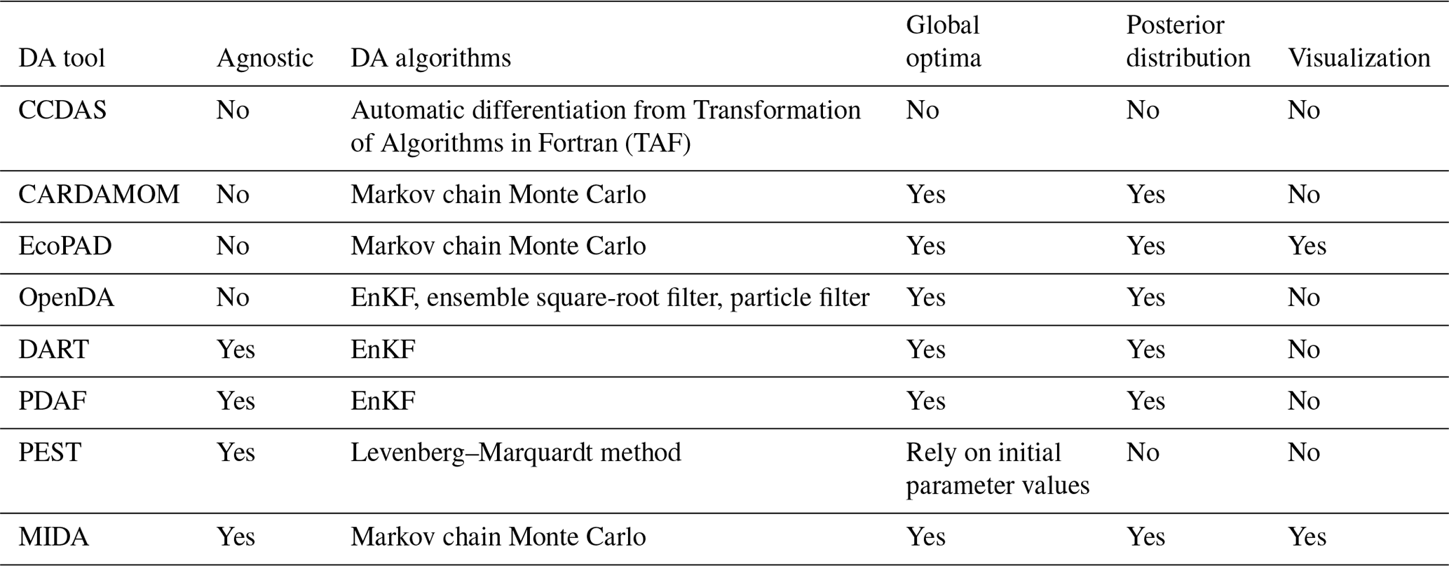
A number of tools have been developed to facilitate DA applications (Table 1) but many of them are model dependent, such as the Carbon Cycle Data Assimilation Systems (CCDAS) (Rayner et al., 2005; Scholze et al., 2007), the Carbon Data Model Framework (CARDAMOM) (Bloom et al., 2016), the Ecological Platform for Assimilating Data (EcoPAD) into model (Huang et al. 2019) and Predictive Ecosystem Analyzer (PEcAn) (LeBauer et al., 2013). These tools combine DA algorithms with a specific model. For example, CCDAS specified the DA algorithm to the Biosphere Energy Transfer Hydrology (BETHY) model (Rayner et al., 2005). The hardcoding feature of aforementioned tools make them inflexible to be applied to different models.
There are some model independent DA tools that are not tailored to a specific model, such as Data Assimilation Research Testbed (DART) (Anderson et al., 2009), the open Data Assimilation library (openDA) (Ridler et al., 2014), the Parallel Data Assimilation Framework (PDAF) (Nerger and Hiller, 2013) and Parameter Estimation & Uncertainty Analysis software suit (PEST) (Doherty, 2004).
However, these model-independent tools suffer from some limitations for a general and flexible DA application. For example, openDA requires users to code three functions to initialize a Java class (Ridler et al., 2014) (Table 1). DART enables incorporating a new model through a range of interfaces (Anderson et al., 2009). It has been successfully applied to atmospheric and oceanic models with currently available interfaces (Anderson et al., 2009; Raeder et al., 2012) and recently to the community land model (Fox et al., 2018). It is likely that users may need to prepare new interfaces for new ecological models to use DART. DART and PDAF adopted the Ensemble Kalman Filter (EnKF) method (Evensen, 2003), which may makes it difficult to obey mass conservation for biogeochemical models. This is because the parameter values estimated by EnKF change each time when new data sets are assimilated (Allen et al., 2003; Gao et al., 2011; Trudinger et al., 2007). The sudden changes in estimated parameter values at time points when data are assimilated by EnKF usually do not reflect reality of biogeochemical cycles in the real world. PEST utilizes the Levenberg–Marquardt method (Levenberg, 1944), which is a local optimization method for parameter estimation. If the relationship between simulation outputs and parameters is highly nonlinear, which is common in ecological models, this method may trap into a locally optimization solution (Doherty, 2004).
In this work, we developed a model-independent DA module (MIDA) to enable a general and flexible application of DA in ecology. MIDA was designed as a highly modular tool, independent of specific models, and friendly to users with limited programming skills and/or technical knowledge of DA algorithms. Additionally, MIDA implemented advanced Markov chain Monte Carlo (MCMC) algorithms for DA analysis which can accurately quantify the parameter uncertainty with informative posterior distribution. The anticipated user community in this initial phase of MIDA development is the biogeochemical modelers who are looking for appropriate parameter estimation methods. In the following Sect. 2, we first introduce the development details of MIDA and its usage. In Sect. 3, we demonstrate the application of MIDA to four different types of ecological models. In Sect. 4, we discuss the strengths and weaknesses of MIDA in ecological modeling, and lastly we give our concluding remarks in Sect. 5.
2.1 Bayes' theorem and DA
Based on Bayes' theorem, DA is a statistical approach to constrain parameter values and estimate their posterior density distributions through assimilating observations into a model. The posterior density distributions p(C|Z) of parameters C for a given observation Z can be obtained from prior density distributions p(C) and the likelihood function p(Z|C):
The prior density distribution p(C) is assumed as a uniform distribution over the parameter range. And the likelihood function is negatively proportional to a cost function, J, as
The cost function measures the misfit between simulation outputs and observations and is described in more detail in Sect. 2.4. The posterior density distribution p(C|Z) is estimated from sampling parameter values to maximize the likelihood function p(Z|C) or minimize the cost function J. DA usually uses a sampling technique, such as Markov chain Monte Carlo (MCMC) in this MIDA. The MCMC algorithm successively generates a new set of parameter values from the prior parameter ranges and requires a model run with these new parameter values. Then the cost function is calculated to determine whether this new set of parameter values will be accepted or not according to the Metropolis–Hastings criterion (see more description in Sect. 2.4). All accepted parameter values are used to generate posterior distributions where the distinctive mode indicates the parameter uncertainty is well constrained. Meanwhile, we derive maximum likelihood estimates (MLEs) of parameters from the posterior density distributions.
MIDA realizes model-independent Bayesian-based DA to estimate posterior density distributions and MLEs of parameters via data exchanges between a given model and DA algorithm.
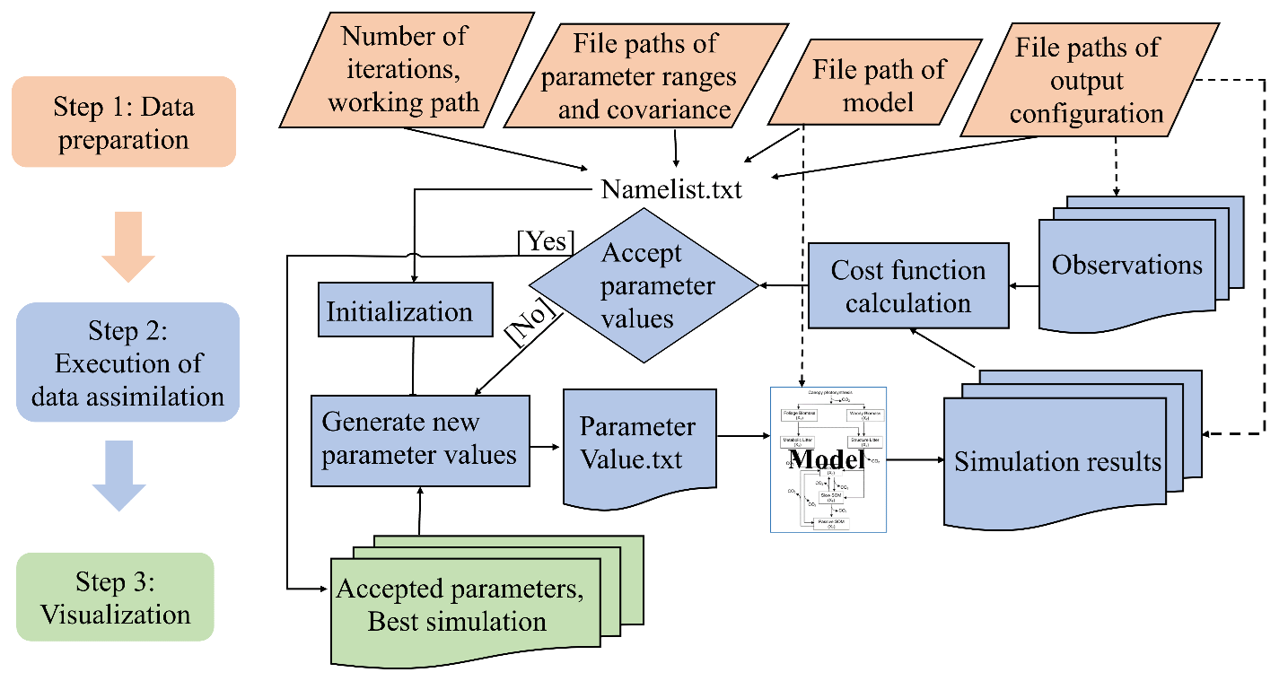
Figure 1The three-step workflow of the Model Independent Data Assimilation (MIDA) module. The workflow includes data preparation, execution of data assimilation (DA), and visualization. The data preparation step is to provide all the formatted essential data for DA via user input. The execution step is to calibrate parameter values towards a constrained posterior distribution with the fusion of observations. The visualization step is to diagnose the effects of DA. The rhombus in orange represents user-input data. The rectangle represents procedures, and document/multidocument shape is for data files in computers. Dashed lines indicate locations of data. Solids lines indicate data flow pathways. With the three-step workflow, DA is agnostic to specific models, and users will be released from technical burdens.
2.2 An overview of MIDA
MIDA is a module that allows for automatic implementation of data assimilation without intrusive modification or coding of the original model (https://doi.org/10.5281/zenodo.4762725, Huang, 2021). Its workflow includes three steps: data preparation, execution of data assimilation, and visualization (Fig. 1). Step 1 (data preparation) is to establish the standardized data exchange between the DA algorithm and the model. Step 2 (execution of data assimilation) is to run DA as a black box independent of the model. Step 3 (visualization) is to diagnose parameter uncertainty after DA. The modularity of the three-step workflow is designed to enable MIDA for a rapid DA application and adaption to a new model. In the following, we introduce the three-step workflows of MIDA, its technical implementation, and its usage in detail.
2.3 Step 1: data preparation
Step 1 is designed to initialize data exchange to transfer parameter values, model outputs, observations, and their variances between the DA algorithm and the model to be used. Four types of information are required either from interactive input or by modifying the “namelist.txt” file (Fig. 1). The first type is about DA configuration, including the number of sampling series in DA and the working path where the outputs of DA will be saved. The number of a sampling series is essential in a DA task to define how many times parameter values are sampled to run the model. The second type of information is about parameter ranges and their covariance. The third is the model executable file. Finally, the fourth type is an output configuration file which contains the file paths of model outputs, observations, and their variance. This file also instructs how to read model outputs and compare each output with corresponding observations.
Traditional DA requires users to modify the code of the model to incorporate the process of data exchange between the DA algorithm and the model. Therefore, the program of data exchange in traditional DA is model-specific, and users need to repeat such a program when a new model comes. In MIDA, the process of data exchange calls a model executable file which hides the details of the model code. When applied to a new model, MIDA only requires users to provide a different model executable file in the namelist.txt file and does not involve any additional coding in either the model or MIDA. Thus, MIDA lowers the technical barrier for general ecologists to conduct DA.
Traditional DA usually presets the number of parameters and the model outputs according to a specific model before initializing the data exchange. This is because data exchange between the DA algorithm and model uses memory to transfer items such as parameter values. Instead, MIDA organizes items in data exchange using different files. Items in data exchange are decided by the data file loaded when MIDA is running. The number of parameter values, for example, will be decided after the file of parameter range is read in MIDA. Through modifying files, MIDA allows efficient choices about the model-related items in data exchange to be made. Thus, MIDA is highly flexible and modular for DA with different models.
Traditional DA also presets observation types in the data exchange according to a specific study before the data exchange. For example, if the traditional DA uses carbon flux observation, it cannot switch to satellite remote sensing products without additional coding. MIDA uses the concepts of object-orient programming (Mitchell and Apt, 2003) and dynamic initialization (Cline et al., 1998) in computer science to provide a homogenous way to create various observation types from a unified prototype class. A prototype class includes variables to store observations and their variance and functions (e.g., read from observation files). The values in variables are dynamically decided after the observation files are loaded when MIDA is running. Different observation types derive from the prototype class with a high degree of reusability of most functions. In such a way, MIDA only requires users to provide different filenames of the observations to be integrated in DA. Therefore, MIDA is highly flexible and modular for DA to assimilate various observations.
2.4 Step 2: execution of data assimilation
After the establishment of the standardized data exchange (step 1), step 2 is to run DA as a black box for users without knowledge of DA itself. Notwithstanding the black-box goal, this section provides a general description of DA below.
Data assimilation as a process integrates observations into a model to constrain parameters and estimate parameter uncertainties. Data assimilation usually uses some types of sampling algorithms, such as Markov chain Monte Carlo (MCMC), to generate posterior parameter distribution under a Bayesian inference framework (Box and Tiao, 1992). As mentioned in Sect. 2.1, DA with a MCMC algorithm estimates the posterior density distributions through sampling to maximize likelihood function p(Z|C) or minimize the misfit J between simulation outputs and observations. This version of MIDA uses the MCMC algorithm implemented by the Metropolis–Hastings (MH) sampling method (Hastings, 1970; Metropolis et al., 1953). The future version of MIDA could incorporate other data assimilation algorithms. Each iteration in the Metropolis–Hastings sampling includes a proposing phase and a moving phase. The proposing phase generates a new set of parameter values based on the starting point for the first iteration or current accepted parameter values in the following iterations. If parameter covariance (covparam) is specified in step 1 on data preparation, this proposing phase will draw new parameter values (Cnew) within the prior ranges from a Gaussian distribution N(Cold,covparam), where Cold is the predecessor set of parameter values. Without parameter covariance, a new set of parameter values will be generated from a uniform distribution within the prior ranges (Xu et al., 2006).
The moving phase first calculates mismatches between observations and the model simulation with the new set of parameter values as a cost function (Jnew in Eq. 3) (Xu et al., 2006):
where n is the number of observations, Zi(t) is the ith observation at time t, Xi(t) is the corresponding simulation, and is the variance of the observation. The error is assumed to independently follow a Gaussian distribution. This new set of parameter values will be accepted if Jnew is smaller than Jold, the cost function with the previous set of accepted parameter values, or the value, , is larger than a random number selected from a uniform distribution from 0 to 1 according to the Metropolis criterion (Liang et al., 2018; Luo et al., 2011; Shi et al., 2018; Xu et al., 2006). Once the new set of parameter values is accepted, Jnew becomes Jold. Those two phases of sampling will be iteratively executed until the number of sampling series set in step 1 on preparation of DA is reached. Finally, the posterior density distributions can be generated from all the accepted parameter values.
MIDA realizes the execution of data assimilation according to the procedure described above. First, MIDA uses a “call” function to execute model simulations to get values of Xi(t). Observations Zi(t) and their variance are already provided via the standardized data exchange as described in step 1. Then, MIDA calculates Jnew according to Eq. (3) to decide the acceptance of the current parameter values used in this simulation. If accepted, MIDA saves this set of parameter values and associated Jnew values in Caccepted and Jaccepted array, respectively, and triggers a new proposing phrase based on this set of accepted parameter values. If not, MIDA discards this set of parameter values and generates another new set of parameter values. MIDA saves the new parameter values generated in the proposing phrase to “ParameterValue.txt”, from which the model reads before execution of the next model simulation. MIDA repeats the proposing and moving phases until the number of sampling series is reached. At the end, MIDA selects the best parameter values through maximum likelihood estimation and runs the model again using this set of values to get optimized simulation outputs Xi(t). Then MIDA saves the arrays of accepted parameters, associated errors, maximum likelihood estimates (MLEs), and optimized state variables Xi(t) to four files, “parameter_accepted.txt”, “J_accepted.txt”, “MLE.txt”, and “OptimizedSimu.txt”, respectively.
This execution of the DA algorithm in MIDA enables users to conduct DA as a black box and is independent of any particular model.
2.5 Step 3: visualization
Step 3 is to visualize the results of DA in step 2. The end products of DA are accepted parameter values, their associated Jnew values, the maximum likelihood estimates, and optimized simulation results as saved in the output files. MIDA enables visualization of parameter posterior density distributions with a Python script. In the script, MIDA first read accepted parameter values from the parameter_accepted.txt file. Then, MIDA generates a posterior probabilistic density function (PPDF) for each parameter via the “kdeplot” function in the “seaborn” package. The maximum likelihood estimates of parameters correspond to the peaks of PPDF. The distinctive mode of PPDF indicates how well the parameter uncertainty is constrained. Finally, MIDA visualizes the PPDF for all parameters in a figure using the “matplotlib” package.
2.6 Implementation and architecture of MIDA
MIDA is equipped with a graphical user interface (GUI), and users can easily execute it through an interactive window. Users can also run MIDA as a script program without the GUI. MIDA is written in Python (version 3.7). For the GUI-version, all relevant Python packages used in MIDA are compiled together; thus users do not need to install them by themselves. For the non-GUI version, users need to install Python 3.7 and relevant packages (i.e., numpy, pandas, shutil, subprocess, matplotlib, math, os, and seaborn). MIDA is compatible with model source codes written in multiple programming languages (e.g., Fortran, C/C, C#, MATLAB, R, or Python). It is also independent of multiple operation systems (e.g., Windows, Linux, MacOS). In addition, MIDA is also able to run on high-performance computing (HPC) platforms via task management systems (e.g., Slurm).
The architecture of MIDA is class-based, and each class is designed to describe an object (e.g., parameter, observations) with variables and operations. Five classes are defined in MIDA: parameter, observation, initialization, MCMC algorithm, and the main program. The main program is the start of MIDA execution. It calls functions from all other classes to finish a three-step workflow. As described in Sect. 2.2, parameter and observation classes contain variables to be transferred in data exchanges via file I/O operations. These operations are implemented using the “numpy” package. The initialization class is to read namelist.txt in step 1 on data preparation and to assign values for the variables in all other classes. Then the class of MCMC algorithm conducts DA as described in step 2. In this step, the simulation operation uses a call function in the “subprocess” package to call the model executable file. At the start of model simulation, MIDA writes new parameter values to the “ParameterValue.txt” file in the “working path” directory specified in step 1 on data preparation. Then model executable reads parameter values from the ParameterValue.txt file and run. After model simulation, the DA algorithm can read the model outputs by the output filenames indicated in the output configuration file. After DA, step 3 executes an additional Python script to read accepted parameter values and plot the posterior density distributions of parameters. The plotting operations use the matplotlib and seaborn packages. The implementation of GUI uses the pyQt5 toolkit to support interactive usage of MIDA. Users can also run MIDA in a non-interactive way with a “main.py” script to trigger the three-step workflows.
2.7 User information of MIDA
In order to use MIDA, users need to prepare data and a model. The data to be used in MIDA are prior ranges and default values of parameters, parameter covariances, output configuration file, observations, and their variances. They are organized in different files. Before running MIDA, users need to specify their filenames as suggested in step 1. When users want to use different data sets in DA, they can simply change filenames with the new data sets via GUI or in the namelist.txt file. Figure C1 is an example of the namelist.txt file for a data assimilation study with the DALEC model. The model to be used in MIDA should have those to-be-estimated parameter values not fixed in model source code rather than changeable through ParameterValue.txt file. MIDA writes new parameter values in each proposing phase during DA to the ParameterValue.txt file, from which the model reads the parameter values to run the simulation.
To calculate the cost function, J, we have to have a one-to-one match between observations and model outputs. For example, phenology models in one of the application cases of MIDA below generate discrete dates of leaf onset, which is a one-to-one match to the observations of spring leaf onset. In this case, observation Zi(t) and model output Xi(t) to be used in calculation of J are straightforward. In the application case for dynamic vegetation, the data to be used are leaf area in six layers in a forest 302 years old, whereas the model simulates leaf areas in eight layers from 0 to 800 years. To match observation, the model generates outputs of leaf areas in six layers when simulated forest age reaches 302 years. This requires users to prepare an output configuration file to instruct MIDA to read model outputs and re-organize their outputs to match observation. The output configuration file starts with a single line listing an observation filename and its corresponding output filenames. Content after the directories in the output configuration file are instructions to map model outputs with the observation signified in the first line. Each instruction is to match one or continuous elements in observation with elements in outputs with the same length. A blank line means there are no further instructions. Then a new matching between another observation and model outputs starts. An example of output configure file is available in Appendix B.
Once MIDA finishes the execution of data assimilation, users may need basic knowledge to assess the performance of DA. For example, the acceptance rate, which is given by MIDA, is the fraction of proposed parameter values that is accepted. Ideally, the acceptance rate should be about 20 %–50 % (Xu et al., 2006). A very low acceptance rate indicates that many new proposed parameter values (Cnew) are rejected because Cnew jumps too far away from the previously accepted parameter values (Robert and Casella, 2013; Roberts et al., 1997). In this case, users are suggested to reduce a jump scale in the proposing phase. On the other hand, a very high acceptance rate is likely because Cnew moves slowly from the previously accepted parameter values. Users may increase the jump scale.
In addition, DA usually requires a convergence test to examine whether posterior distributions from different sampling series converge or not. A convergence test requires running DA parallelly or multiple times with different initial parameter values. MIDA provides a Gelman–Rubin (G–R) test (Gelman and Rubin, 1992) for this purpose. To use the G–R test, users need to prepare a file containing initial parameters values in different sampling series and indicate its filename in the namelist.txt file as described in step 1. If the G–R statistics approaches 1, the sampling series in DA is converged. When the sampling series is converged, all accepted parameter values are used to generate the posterior distributions.
There are three types of posterior distributions: bell shape, edge hitting, and flat. The bell-shaped posterior distributions indicate that these parameters are well constrained. Their peak values are the maximum likelihood estimates of parameter values. The flat posterior distributions suggest that the parameters are not constrained due to the lack of relevant information in data. The edge-hitting posterior distributions result from complex reasons, such as improper prior parameter range. Users may change the prior ranges to examine whether those posterior distributions can be improved or examine correlations among estimated parameters.
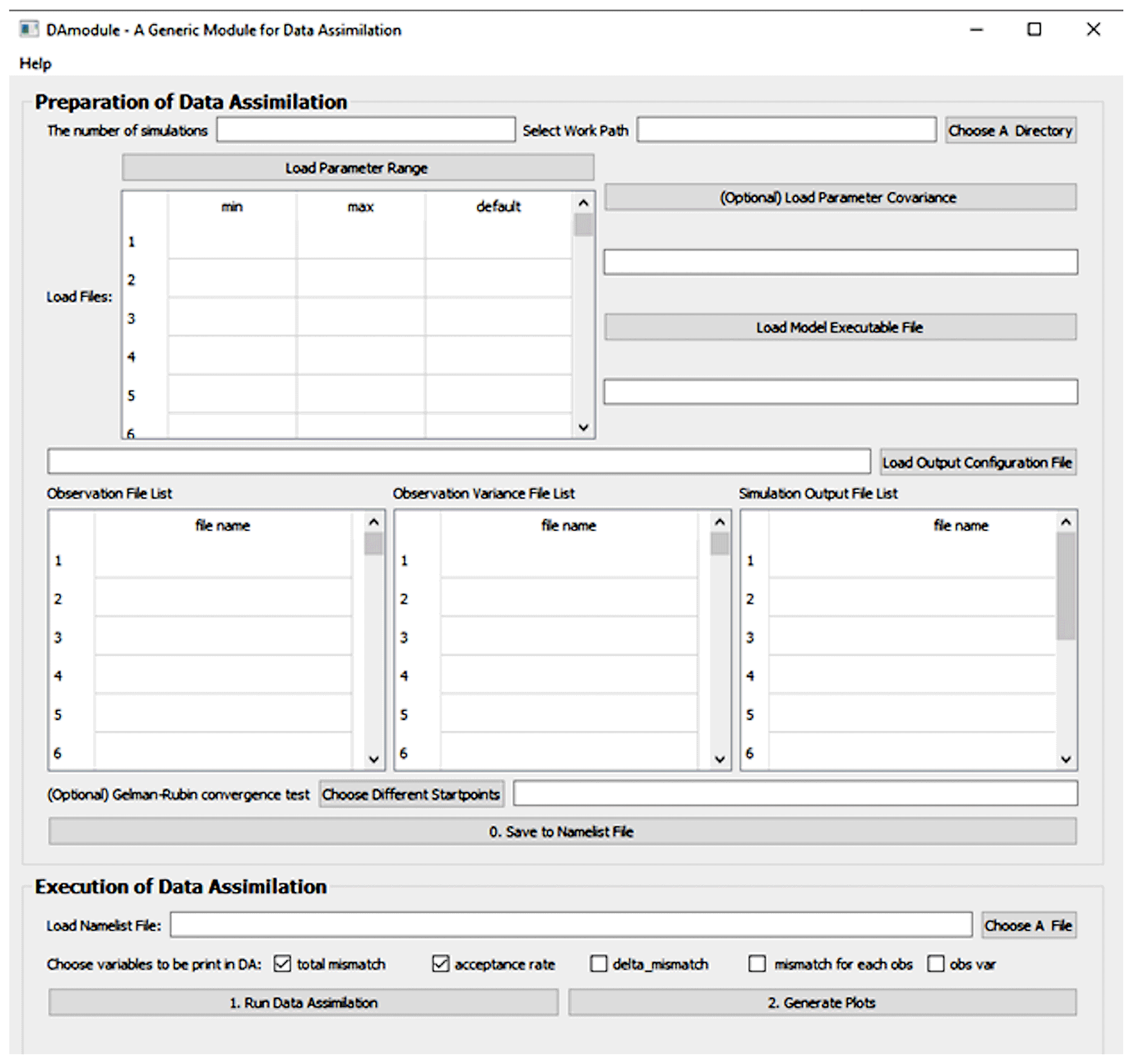
Figure 2The GUI-MIDA window includes two panels. The upper panel is to set up a data assimilation task. Inputs can be loaded and applied to step 1 on data preparation for DA. The lower panel is to run DA as described in step 2 and visualize the posterior distributions of parameters in step 3.
We applied MIDA to four groups of models, which are an ecosystem carbon cycle model, a surrogate-based land surface model, nine phenology models, and a dynamic vegetation model. These four cases demonstrate that MIDA is effective for stand-alone DA, flexible to be applied to different models, and efficient for multiple model comparison.
3.1 Case 1: independent data assimilation with DALEC
The first case study is to demonstrate that MIDA can be effective for independent data assimilation with the data assimilation linked ecosystem carbon (DALEC) model (Lu et al., 2017). DALEC has been used for data assimilation in several studies (Bloom et al., 2016; Lu et al., 2017; Richardson et al., 2010; Safta et al., 2015; Williams et al., 2005). Previous studies all incorporated data assimilation algorithms into DALEC, which requires invasive coding. This case study is focused on reproducing the data assimilation results as in the study by Lu et al. (2017) but with MIDA.
The version of DALEC used in this study is composed of six submodels (i.e., photosynthesis, phenology, autotrophic respiration, allocation, litterfall, and decomposition) to simulate the carbon exchanges among five carbon pools (i.e., leaf, stem, root, soil organic matter, and litter) (Ricciuto et al., 2011). There are 21 parameters in DALEC, of which 17 parameters are derived from the six submodels and four parameters serve to initialize the carbon pools. Table 2 summarizes the names, prior ranges, and nominal values of these 21 parameters. The observation is the Harvard Forest daily net ecosystem exchange (NEE) from the years 1992 to 2006. DALEC is coded in Fortran. In a Windows system, a gfortran compiler converts the model code to an executable file (i.e., DALEC.exe).
Table 2A summary of 21 parameters to be calibrated in the DALEC model. The default parameter value and prior parameter range are shown.
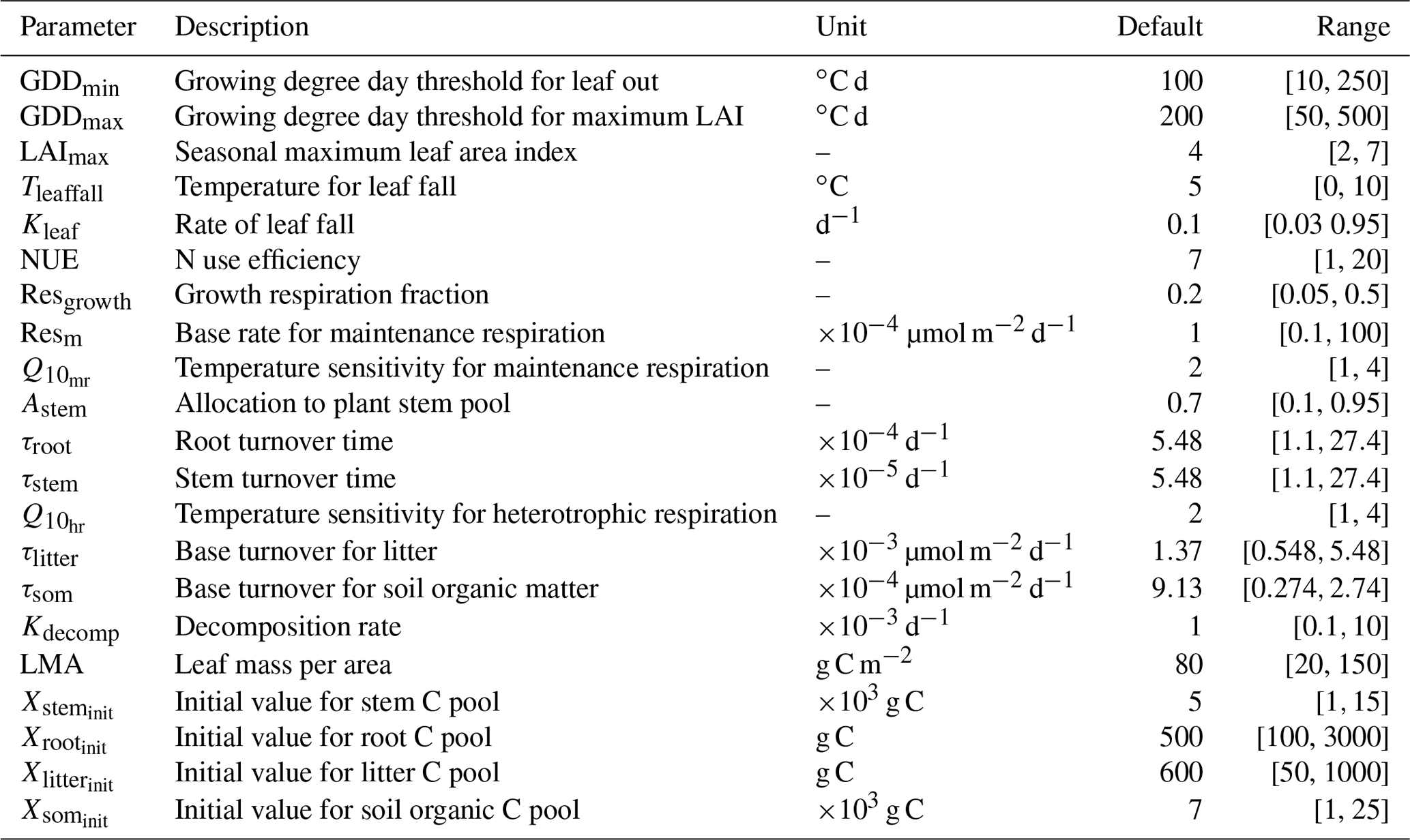
Figure 2 is the GUI window of MIDA. We first set up a DA task as described in step 1 using the upper panel. In this application, the number of sampling series is set as 20 000. Once users click the “choose a directory” or “choose a file” button, a new dialog window will pop up and users are able to choose the directory or load files interactively. As describe in step 1 on preparation of DA, the working path is where the outputs of DA and ParameterValue.txt are saved (e.g., C:/workingPath). After the output configuration file is loaded, the filenames of model outputs, observations, and their variance will be displayed in the window automatically. This application only uses a “NEE.txt” observation file. Similarly, after users load the parameter range file (e.g., a file named “ParamRange.txt” contains three rows which are minimum, maximum, and default values of parameters), the content in this file is displayed as well. To replace the current parameter range file loaded, users can simply upload another file. In this application, the executive model file is “DALEC.exe” with a Fortran compiler in a Windows system. Because we do not have parameter covariance information, this input is left blank. After “save to namelist file” is clicked, a namelist.txt file containing all the inputs will be generated in the working path.
After the DA task setup, we load the namelist.txt file and click the “run data assimilation” button in the lower panel to trigger step 2 on execution of DA. A new dialog will pop up to show the acceptance rate information and notify the termination of DA. Then we will click the “generate plots” button to visualize the posterior distributions of 21 parameters as described in step 3.
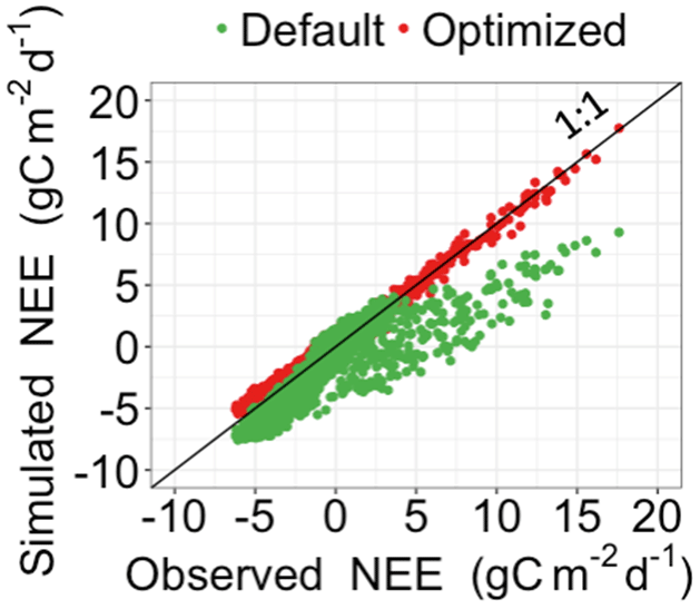
Figure 3Comparison between the simulated daily net ecosystem exchange (NEE) by DALEC and the observed NEE at Harvard Forest from 1992 to 2006. Red circles represent modeled NEE with the optimized parameter values, and green circles represent simulated NEE with the original parameter values. Simulations of DALEC are substantially improved after data assimilation in comparison with those before data assimilation.
Figure 3 shows that the simulation outputs using the optimized parameter values from MIDA better fit with the observations than those using default parameter values. Figure 4 depicts posterior distributions of the 21 parameters estimated from MIDA. More than half of the parameters are constrained well with a unimodal shape. and have a wide occupation of the prior range, indicating that the observation data do not provide useful information for them. The constrained posterior distributions in this study are similar to those from Lu et al. (2017). Note that MCMC estimates have a large variance and a low convergence rate, especially in high-dimensional problems; with a finite number of samples it is not expected that two simulations would give exactly the same results.
3.2 Case 2: application of MIDA to a surrogate land surface model
This case study is to examine the applicability of MIDA to a surrogate-based land surface model. The original model is Energy Exascale Earth System Model: the Land Component (ELM) (Ricciuto et al., 2018). As ELM is computationally expensive (one forward model simulation takes more than 1 d), a sparse-grid (SG) surrogate system was developed to reduce the computational time (Lu et al., 2018). The forcing data for the surrogate model is half-hourly meteorological measurements at the Missouri Ozark flux site from 2006 to 2014. The observations that were used for optimization are annual sums of net ecosystem exchange (NEE), annual averages of total leaf area index, and latent heat fluxes from 2006 to 2010. The eight parameters selected (Table 3) are the most important parameters for the variations in outputs (Ricciuto et al., 2018). The model is written in Python. A “pyinstaller” library packages the model code into an executable file. The iteration number in MIDA is 20 000.
Table 3A summary of eight parameters to be calibrated in the surrogate-based ELM model. The default parameter value and prior parameter range are shown.
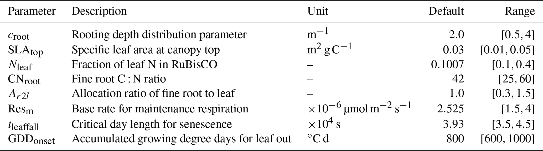
Figure 5 shows posterior distributions of calibrated parameters. croot, SLAtop, tleaffall, and GDDonset are constrained well with a unimodal distribution. However, the distribution of the other four parameters (i.e., Nleaf, CNroot, Ar2l, and Resm) clusters near the edge. These results match well with the study by Lu et al. (2018). As shown in Fig. 6, the calibrated parameters induce a performance improvement in simulating total leaf area index and NEE. For latent heat, both the default and optimized simulation obtain good agreement with the observation. These conclusions are also similar to those in Lu et al. (2018).
MIDA hides the detailed differences between models. For example, the DALEC model in case 1 is a process-based model to simulate the ecosystem carbon cycle while surrogate-based ELM in case 2 is an approximation of a land surface model. They are also different in programming language, simulation time, forcing data, etc. MIDA is able to deal with models with so many different characteristics and hides these differences from users. Users only need to indicate the filenames of the model to be used, its parameter range, the output configuration file, etc. in the namelist.txt file. Thus, MIDA simplified the DA applications using different models.
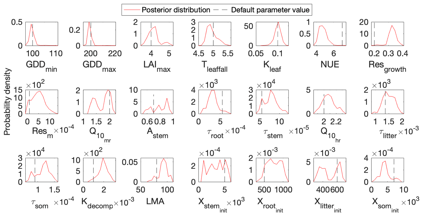
Figure 4Comparison between posterior distributions (red line) and default values (gray dash line) of the 21 parameters in DALEC. The peak in posterior distribution is the constrained parameter value from the maximum likelihood estimation. This distinctive mode and its divergence from the default value indicates the effects of DA. Most parameters are well constrained, and some are far different from the original values.
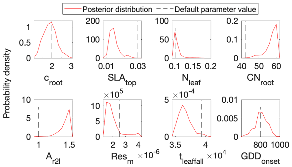
Figure 5Comparison between posterior distributions (red line) and default values (gray dash line) of the eight parameters in surrogate-based ELM. The peak in posterior distribution is the constrained parameter value from maximum likelihood estimation. This distinctive mode and its divergence from the default value indicate the effects of DA. Most parameters are well constrained, and some are far different from the original values.
3.3 Case 3: evaluation of multiple phenological models
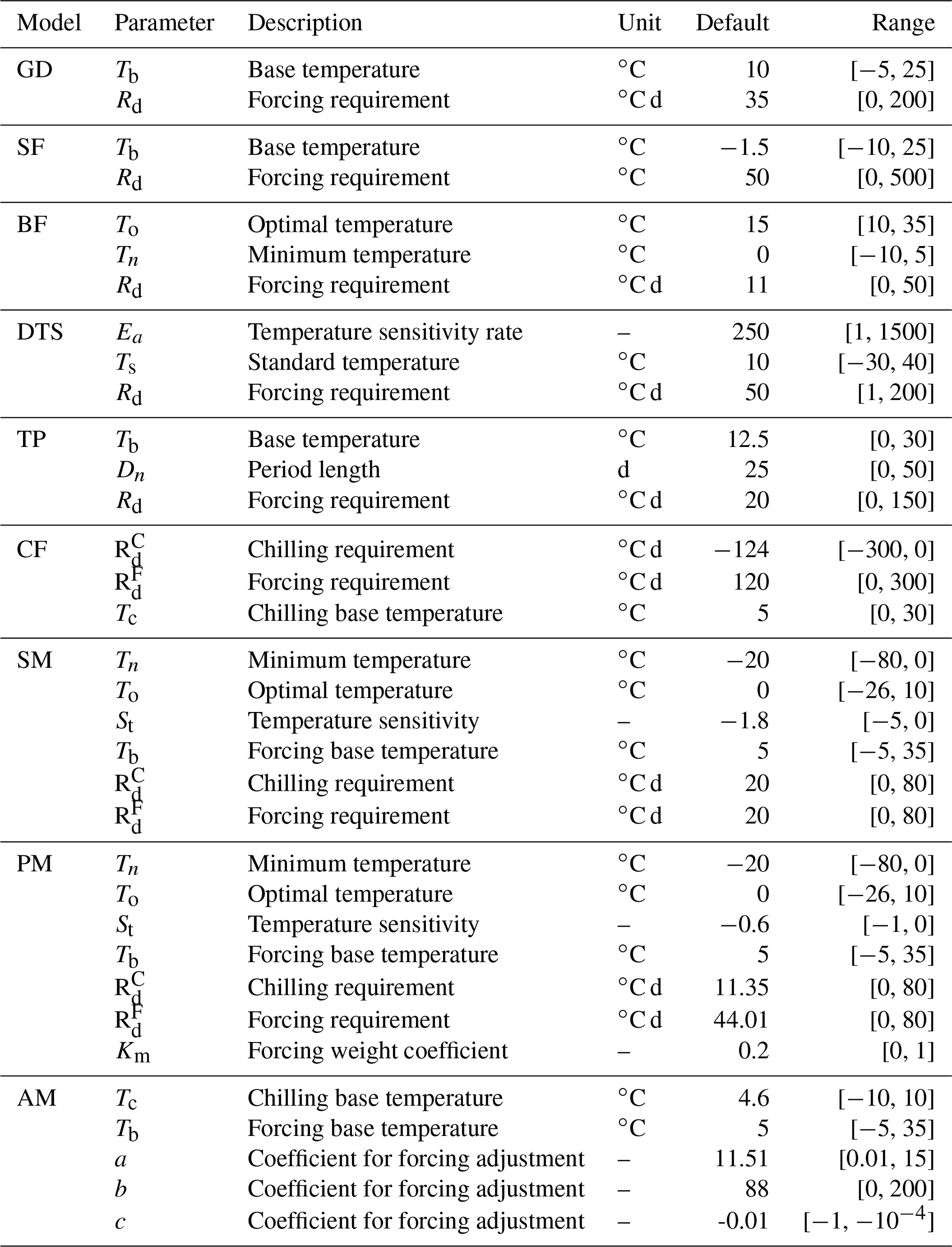
This study case uses nine phenological models (Yun et al., 2017) to demonstrate the applicability of MIDA in model comparison. Five out of the nine models predict phenological events, such as the day of leaf onset, using growing degree days, which are calculated as temperature accumulation above a base temperature. The other four models consider two processes: chilling effects of cold temperature on dormancy before budburst and forcing effects of warm temperature on plant development. Each model uses different response functions to represent chilling and forcing effects. The detailed model descriptions and associated parameter information are in the Supplement table.
Data are from the Spruce and Peatland Responses Under Climatic and Environmental Change experiment (SPRUCE) (Hanson et al., 2017) located in northern Minnesota, USA. The experiment consists of five-level whole-ecosystem warming (i.e., +0, +2.25, +4.5, +6.75, +9 ∘C) and two-level elevated CO2 concentrations (i.e., +0, +500 ppm). Dates of leaf onset were observed with PhenoCam (Richardson et al., 2018) for tree species Picea mariana and Larix laricina. For the sake of demonstration of MIDA application, we only show DA results for Larix laricina with +9 ∘C warming treatment and +0 ppm CO2 treatment from 2016 to 2018.
MIDA was used to compare performances of the nine models in reference to the same observations of leaf onset dates after DA. We as users changed filenames of model executable files (i.e., PhenoModels.exe), defined parameter ranges, and assigned the directory of working path for each model. MIDA then estimated the optimized parameters and saved the corresponding best simulation outputs to the working path for each of the nine models. Figure 7 shows the best simulation output of these nine models. The simulation output of the sixth, seventh, eighth, and ninth models better fits the observation than the other models. It demonstrates that models that consider both chilling and heating effects can achieve good simulations of the leaf onset dates.

Figure 6Comparison between the simulated NEE, total leaf area index, latent heat flux by surrogate-based ELM, and the observed ones at Missouri Ozark flux site from 2006 to 2014. The blue lines indicate the observations, and their 95 % confidence interval is in the shaded area. The green and red lines indicate the simulations with default parameter values and optimized values, respectively. Simulations are generally improved after DA for all three variables.
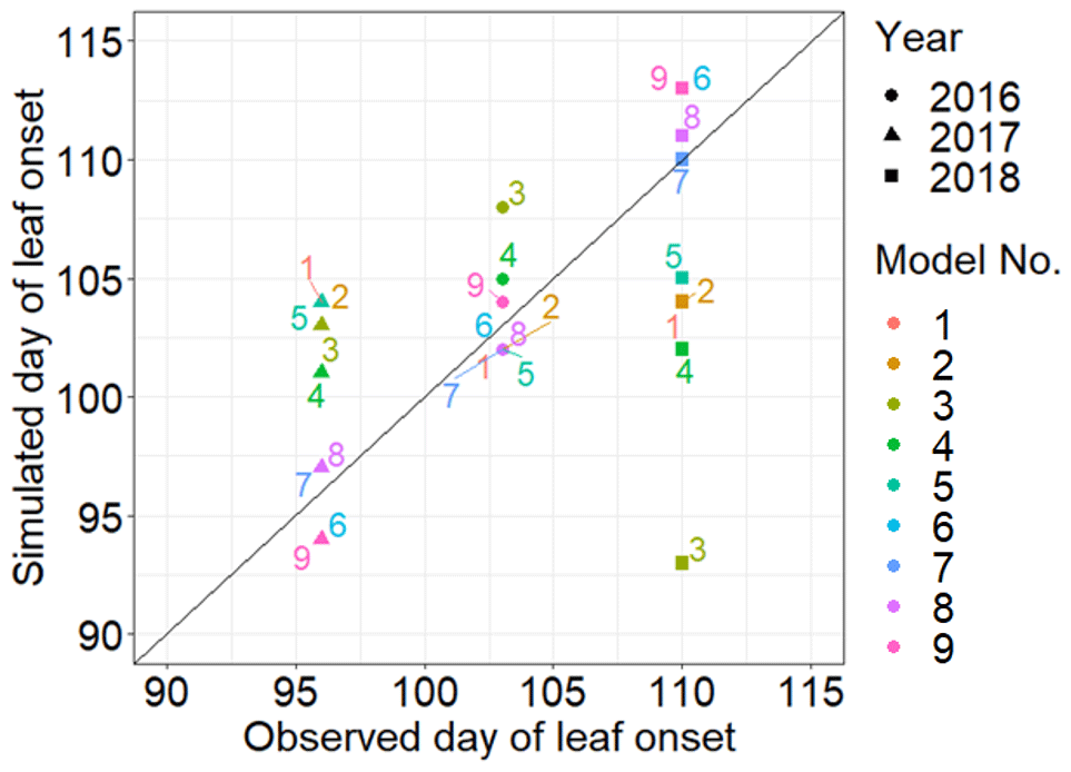
Figure 7Comparison between the simulated growth date by nine phenology models after DA and the observed growth date for Larix laricina with +9∘ treatment at the SPRUCE site from 2016 to 2018. The colored number indicates different models, and shape represents different year. Overall, models 6, 7, 8, and 9 achieve better performance after DA.
3.4 Case 4: supporting data assimilation with a dynamic vegetation model
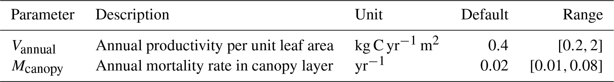
This case study is to examine the efficiency of MIDA to integrate remote sensing data into a dynamic vegetation model. The model used in this study is Biome Ecological strategy simulator (BiomeE) (Weng et al., 2019). This model simulates vegetation demographic processes with individual-based competition for light, soil water, and nutrients. Individual trees in BiomeE model are represented by cohorts of trees with similar sizes. The light competition among cohorts is based on their heights and crown areas according to the rule of perfect plasticity approximation (PPA) model (Strigul et al., 2008). Each cohort has seven pools: leaves, roots, sapwood, heartwood, seeds, nonstructural carbon, and nitrogen. After carbon is assimilated into plants via photosynthesis, the assimilated carbon enters the nonstructural carbon pool and is used for plant growth (i.e., diameter, height, crown area) and reproduction according to empirical allomeric equations (Weng et al., 2019). In this application, two parameters to be constrained (Table 4) are annual productivity rate and annual mortality rate of trees.
Table 4A summary of two parameters to be calibrated in the BiomE model. The default parameter value and prior parameter range are shown.
Observations to be used in DA are leaf area indexes in six vertical heights (i.e., 0–5, 6–10, 11–15, 16–20, 21–25, and 26–30 m) at the Willow Creek study site, Wisconsin, USA. The forest at the site is an upland deciduous broadleaf forest around 302 years old. The observations were from Global Ecosystem Dynamics Investigation (GEDI) acquired by a light detection and ranging (lidar) laser system, which is deployed on the International Space Station (ISS) by NASA in 2018 (Dubayah et al., 2020). The observations were first averaged from three footprints, and then leaf area indexes in the six canopy layers were standardized to be summed up as 1.
To use MIDA, we reorganized the simulation outputs to match observations as suggested in Sect. 2.6. The BiomeE model simulates leaf areas in eight layers (i.e., 0–5, 6–10, 11–15, 16–20, 21–25, 26–30, 31–35, and 36–40 m) from 0 to 800 years. An output configuration file was provided to post-process model outputs of leaf area indexes in six layers to match observations at the forest age of 302 years. These simulated leaf area indexes in the six canopy layers were also standardized to match standardized observations of leaf area indexes. The observations and post-processed simulation outputs were saved to “LAI.txt” and “simu_LAI.txt” files, respectively. The two files are used in MIDA for data assimilation to generate posterior distributions of the two estimated parameters as shown in Fig. 8. The optimized parameter values through maximum likelihood estimation are different from their default values. Figure 9 compares the simulation outputs with optimized parameters estimated by MIDA to those with default parameter values. After DA with GEDI data in MIDA, the simulation accuracy of leaf area index is substantially improved, especially in middle (16–20 m) and highest (26–30 m) layers.
This study introduced MIDA as a model-independent tool to facilitate the application of data assimilation in ecology and biogeochemistry. The potential user community is ecologists with limited knowledge of model programming and technical implementation of DA algorithms. Several model-independent DA tools have already been developed, such as DART (Anderson et al., 2009), openDA (Ridler et al., 2014), PDAF (Nerger and Hiller, 2013), and PEST (Doherty, 2004), mainly for applications in the research areas of hydrology, atmosphere, and remote sensing. These DA tools either use the gradient descent method, such as the Levenberg–Marquardt algorithm in PEST, or Kalman filter methods, such as EnKF in DART, openDA, and PDAF. The Levenberg–Marquardt algorithm is a local search method, for which it is hard to find a global optimization solution for highly nonlinear models. EnKF updates state variables and parameter values each time when observations are sequentially assimilated, resulting in discrete values of estimated parameters. Jumps in estimated parameter values by EnKF make it very difficult to obey mass conservation in biogeochemical models (Gao et al., 2011). In this study, we used the MCMC method in MIDA to generate parameter values and their posterior distributions. MCMC is a widely used method in many DA studies with biogeochemical models but has been applied to individual models with invasive coding (Bloom et al., 2016; Hararuk et al., 2015; Liang et al., 2018; Luo and Schuur, 2020; Ricciuto et al., 2011). Compared to the other model-independent DA tools mentioned above, MIDA is the first tool that uses the MCMC method for DA.
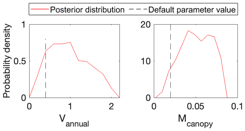
Figure 8Comparison between posterior distributions (red line) and default values (gray dash line) of the two parameters in BiomeE. The peak in posterior distribution is the constrained parameter value from maximum likelihood estimation. This distinctive mode and its divergence from the default value indicate the effects of DA. All parameters are well constrained and different from their original values.
Biogeochemical models are incorporating more detailed processes related to carbon and nitrogen cycles (Lawrence et al., 2020). Complex biogeochemical models yield predictions with great uncertainty (Frienlingstein et al., 2009, 2014). Data assimilation has been increasingly used to estimate parameter values against observations and reduce uncertainty in model prediction (Luo et al., 2016; Luo and Schuur, 2020). However, current applications of DA are almost all model dependent. This requires ecologists to write code to integrate the DA algorithm into models. The coding practice is a big technical challenge for ecologists with limited programming ability. The distinct advantage of MIDA is to enable ecologists to conduct model-independent DA. MIDA streamlines workflow of the three-step procedure for DA to enable users to conduct DA without extensive coding. Users mainly need to provide numerical and character values for data exchanges to transfer data (i.e., parameter values, simulation outputs, observations) between the model and MIDA by a file named namelist.txt or by interactive inputs via a GUI window (Fig. 2).
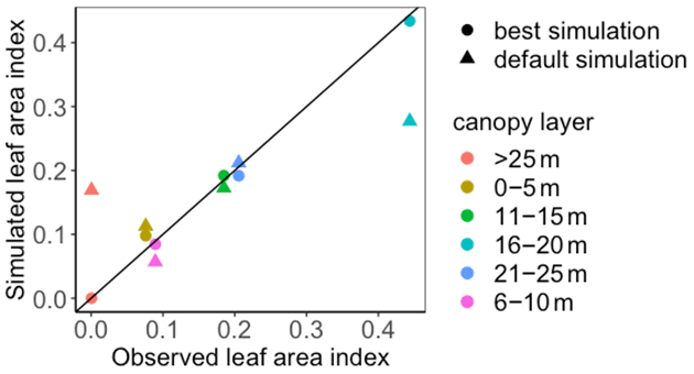
Figure 9Comparison between the simulated leaf area index (LAI) by BiomeE and the observed NEE at Willow Creek. Circles represent modeled NEE with the optimized parameter values, and triangles represent simulated NEE with the original parameter values. Simulations of LAI are substantially improved after data assimilation in comparison with those before data assimilation.
We tested MIDA in four cases for its applicability to ecological models. The first case is applied to the DALEC model, which has been used in several data assimilation studies (Bloom et al., 2016; Lu et al., 2017; Safta et al., 2015; Williams et al., 2005). The previous DA studies all used invasive coding to incorporate the DA algorithm into models. As demonstrated in this study, MIDA was applied to DALEC without invasive coding but by providing the directory to save DA results and filenames of DALEC model executable file, parameter prior range, and output configuration files through the namelist.txt file or interactive inputs in the first preparation step of the workflow. Then, MIDA runs DA as a black box with DALEC before visualizing the DA results. Next, we tested the applicability of MIDA, a surrogate-based ELM model, and a dynamic vegetation model BiomeE. To switch the test case from DALEC to the surrogate-based ELM model and the BiomeE model, we changed the filenames of the model executable file, parameter prior range, and output configuration file in the namelist.txt file for MIDA. This flexibility of MIDA in switching models for DA makes it much easier for model comparisons. We tested this capability of MIDA with nine phenological models to compare alternative model structures. Similarly, MIDA enables efficient switches of observations to be assimilated into models. Users only need to change filenames of observations in the output configuration file. This feature of MIDA makes it easier to utilize abundant trait databases such as TRY (Kattge et al., 2020), FRED (Iversen et al., 2017), etc. Moreover, this feature of MIDA also helps evaluate the relative information content of different observations for constraining model parameters and prediction (Weng and Luo, 2011). Consequently, MIDA can facilitate selection of the most informative observations and then better guide data collections in field experiments. Ultimately, MIDA can aid ecological forecasting and help reduce uncertainty in model predictions (Huang et al., 2018; Jiang et al., 2018).
Although MIDA helps users to get rid of model detail, users may still need basic knowledge about the model outputs to prepare the output configuration file which is to match model outputs to observations one by one (see Sect. 2.6). This effort of preparing the correspondence between model outputs and observations for MIDA is not that difficult because users are reading or writing a text file, and most model developers will provide reference to help understand observations or model output files.
Generally, MIDA requires longer time to run DA than the embedded DA algorithm, because MIDA calls model simulation as an external executable file rather than a function embedded. Thus, we recommend MIDA for beginners of DA users with models that are less complex. Besides, the current version of MIDA only incorporates the Metropolis–Hastings sampling approach. More MCMC methods (e.g., Hamiltonian Monte Carlo) may be incorporated into MIDA in the future.
We developed MIDA to facilitate data assimilation for biogeochemical models. Traditional DA studies require ecologists to program codes to integrate DA algorithms into model source codes. The easy-to-use MIDA module enables ecologists to conduct model-independent DA without extensive coding, thus advancing the application of DA for ecological modeling and forecasting. We demonstrated the capability of MIDA in four cases with a total of 12 ecological models. These cases showed that MIDA is easy to perform for a variety of models and can efficiently produce accurate parameter posterior distributions. Moreover, MIDA supports flexible usage of different models and different observations in the DA analysis and allows a quick switch from one model to another. This capability enables MIDA to serve as an efficient tool for model intercomparison projects and enhancing ecological forecasting.
A1 Growing degree (GD)
The growing degree (GD) model is one of the most widespread phenological models to simulate the date of leaf onset (). In this study, the timescale is limited to daily based on observation records. The kernel of GD is to calculate the growing degree days (GDD, ), which is the heat accumulation above a base temperature (Tb). For simplicity, the daily temperature (Td) can be approximated by the average of daily maximum and minimum temperatures. The heat accumulation starts at day Ds, which is empirically estimated, and ends when GDD reaches a forcing requirement threshold (Rd). Two parameters to be constrained are base temperature (Tb) and the forcing requirement (Rd). Their default values and prior range are listed in Table A1.
A2 Sigmoid function (SF)
Compared to the linear response function of GDD in the GD model, the sigmoid function (SF) model provides a non-linear function to better represent the non-linearity of the growth response to heat accumulation. Three parameters to be constrained in DA are base temperature (Tb), the forcing requirement (Rd), and temperature sensitivity (St). Their default values and prior range are listed in Table A1.
A3 Beta function (BF)
In reality, the plant growth rate, as described with Δd, gradually increases up to a specific temperature and then rapidly declines to a supra-optimal level. Such a response can be well described by a beta function with uni-modality and non-symmetrical shape. Three parameters are involved in DA: minimum temperature (Tn), optimal temperature (To), and forcing requirement (Rd). The other parameter values are fixed with empirical values. For example, maximum growth rate (Rx) is set to 1, and maximum temperature (Tx) is assumed to be 45.
A4 Days transferred to standard temperature (DTS)
According to Arrhenius law, the relationship between growth rate and daily temperature Td can be interpolated by Eq. (A8) (Ono and Konno, 1999). With a factor weighted by standard temperature, the equation for DTS (Eq. A9) can better represent growth rate dependent on temperatures. Three parameters considered in DA are temperature sensitivity rate (Ea), standard temperature (Ts), and forcing requirement (Rd).
A5 Thermal period fixed model (TP)
The difference between GD and TP models is that heat accumulation occurs in a fixed time period (Dn). The day of leaf onset is the last day () when the accumulated heat reaches the forcing requirement. The start day () of heat accumulation begins on day one and moves 1 d forward each time to estimate Eq. (A12). Three parameters are involved in DA: the base temperature (Tb), the period length (Dn), and the forcing requirement (Rd).
A6 Chilling and forcing (CF)
Compared to GD, there is another distinctive chilling period for dormancy. The CF model sequentially calculates two accumulations in opposite directions: chilling accumulation and anti-chilling accumulation. The start day of chilling accumulation (Ds) is implicitly set as 273.0, which is 1 October. The end day of chilling accumulation (D0) is the beginning of anti-chilling accumulation. Three parameters are considered in DA: the chilling requirement (), the forcing requirement (), and the temperature threshold (Tc).
A7 Sequential model (SM)
The difference between CF and SM models is that SM used a beta function (Eq. A18) for the calculation of chilling accumulation and adopted a sigmoid function (Eq. A20) for anti-chilling accumulation. The detailed descriptions of these two functions can be referred to in the introductions of the BF model and CF model. The maximum temperature is empirically set as 13.7695. Six parameters are constrained in DA: minimum temperature (Tn), optimal temperature (To), temperature sensitivity (St), forcing base temperature (Tb), chilling requirement (), and forcing requirement ().
A8 Parallel model (PM)
The critical difference between PM and the above two-step models is that the chilling and anti-chilling accumulations happen simultaneously (Fu et al., 2012). In the earlier dates during the chilling period, only a small fraction (Kd) of forcing (Eq. A25) will be accumulated. The maximum temperature is empirically set as 15.3. Seven parameters will be considered in DA: minimum temperature (Tn), optimal temperature (To), temperature sensitivity (St), forcing base temperature (Tb), chilling requirement (), forcing requirement (), and a forcing weight coefficient (Km).
A9 Alternating model (AM)
The AM fixes the start date of the chilling period () as 1 November and the start date of anti-chilling period () as 1 January. The difference between the AM and the other models above is that the forcing requirement is not a parameter value but is decided by the length of chilling days (Fu et al., 2012). Five parameters to be constrained in DA are chilling temperature (Tc), forcing base temperature (Tb), and three coefficients () in calculation of the forcing requirement.
Table A1A summary of parameters to be calibrated in nine phenological models. Their default parameter value and prior parameter range are shown.
The output configuration file (e.g., config.txt) is to indicate the directories of observations and simulation output files as well as how they map to each other. Figure B1 is an example of the output configuration file. There are three blocks of functions to map simulation outputs to observed gross primary production (GPP), respiration (RE), and net ecosystem exchange (NEE). The blocks of mapping functions are separated by a blank line. Each mapping block starts with the directories of one observation, its observation variance, and model outputs, which are separated by a hash key. If there is no observation variance available, users can ignore this directory. If multiple simulation outputs are used to correspond to one observation, the directories of simulation outputs are separated by a comma. The rest of the mapping block describes how to map simulation outputs to observations. The simu_map variable is simulation output after mapping. The simuList variable saves the simulation outputs specified in the first line. Taking the third mapping block in Fig. B1 as an example, simuList[0] saves contents in simuNEE_1.txt, and simuList[0][0:365] saves the first 365 elements in this file.
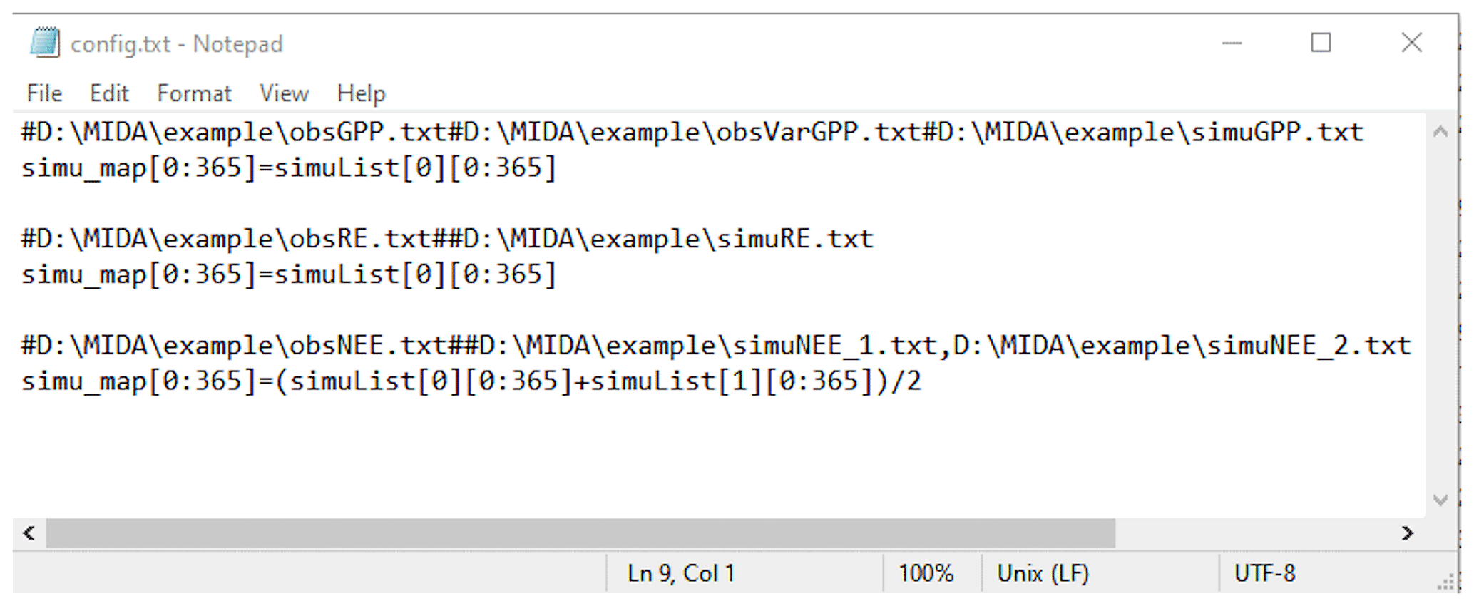
Figure C1 shows an example of the namelist.txt for the first study case with the DALEC model. Users need to prepare the namelist.txt before execution of data assimilation (DA) either manually or via GUI. Below describes the content in the namelist.txt. Detailed explanation and tutorials are available in the Zenodo repositories at the end of the appendixes.
“workpath” is the directory where the MIDA executable files are saved. “nsimu” is the number of iterations in execution of data assimilation. “J_default” is the default mismatch (i.e., cost function) to be compared in the first moving phase of data assimilation. “ProposingStepSize” controls the jump scale in the proposing phase of data assimilation. Users can increase or decrease this value to adjust the acceptance rate to be in a range from 0.2 to 0.5. “paramFile” is the directory of a csv file saving parameter-related information such as parameter range. “obsList” saves the directories of observations. Multiple observations are separated by semicolon. Similarly, “obsVarList” saves the directories of observation variance in the same order as that of obsList. “simuList” saves the directories of simulation outputs corresponding to the observations. With GUI, MIDA reads directories in the output configuration file (e.g., config.txt), which users provide and assign values for obsList, obsVarList, and simuList in the namelist.txt automatically. In this case, if the directories of observations change, users only need to modify the output configuration file and generate the namelist.txt again with GUI-based MIDA.
“paramValue” is the directory of a txt file where MIDA writes out a new set of parameter values for model execution in each iteration of data assimilation. Its default value is ParameterValue.txt under the workpath specified in the first line of the namelist.txt. “model” saves the directory of model executable files. “nChains_convergeTest” indicates whether to conduct a Gelman–Rubin (G–R) convergence test or not. If the G–R test is used, its values are the number of multiple MCMC chains. If not, its value is zero. “convergeTest_startsFile” is the directory of a csv file saving default parameter values as the start points in multiple MCMC chains. “outConvergenceTest” saves the results of the G–R test. If “nChains_ConvergeTest” is zero, both values of “convergeTest_startsFile” and “outConvergenceTest” are empty. “DAresultsPath” is the directory saving the results of DA whose directories are also listed in the following six lines: “outJ” for the accepted mismatches, “outC” for the accepted parameter values, “outRecordNum” for the number of accepted parameter values, “outBestSimu” for the best simulation outputs with the optimal parameter values, and “outBestC” for the optimal parameter values. For MIDA without GUI, “display_plot” indicates whether or not to visualize the posterior distributions after DA.
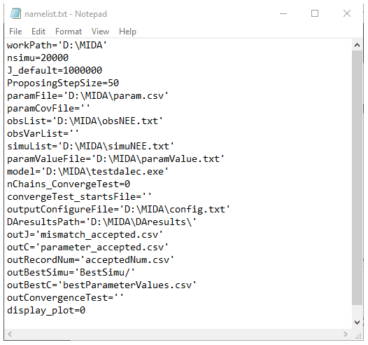
Figure C1An example of the namelist.txt file. In order to use MIDA, users need to prepare data and a model and specify their file names and directories in the namelist.txt file.
The code of MIDA is available at the Zenodo repository https://doi.org/10.5281/zenodo.4762725 (Huang, 2021a). Data used in this study are available at https://doi.org/10.5281/zenodo.4762779 (Huang, 2021b). A comparison of the time cost using the embedded DA algorithm and MIDA is available at the Zenodo repository https://doi.org/10.5281/zenodo.4891319 (Huang, 2021c).
Tutorial videos of how to use MIDA are available at https://doi.org/10.5281/zenodo.4762777.
XH, IS, and YL designed the study. XH built the workflow of MIDA and tested its capability in four cases. DL, DMR, and PJH provided data and models for the first and second test cases. XL prepared models, and ADR provided observations for the third case. EW and SN helped to prepare data and models for the fourth case. XH, LJ, EH, and YL analyzed the results. All authors contributed to the preparation of the manuscript.
The authors declare that they have no conflict of interest.
Publisher’s note: Copernicus Publications remains neutral with regard to jurisdictional claims in published maps and institutional affiliations.
This work was funded by subcontract 4000158404 from Oak Ridge National Laboratory (ORNL) to the Northern Arizona University. ORNL is managed by UT-Battelle, LLC, for the U.S. Department of Energy under contract DE-AC05-00OR22725. Ensheng Weng is supported by the NASA Modeling, Analysis, and Prediction Program (NNH16ZDA001N-MAP).
This paper was edited by Hisashi Sato and reviewed by two anonymous referees.
Allen, J. I., Eknes, M., and Evensen, G.: An Ensemble Kalman Filter with a complex marine ecosystem model: hindcasting phytoplankton in the Cretan Sea, Ann. Geophys., 21, 399–411, https://doi.org/10.5194/angeo-21-399-2003, 2003.
Anderson, J., Hoar, T., Raeder, K., Liu, H., Collins, N., Torn, R., and Avellano, A.: The data assimilation research testbed a community facility, B. Am. Meteorol. Soc., 90, 1283–1296, https://doi.org/10.1175/2009BAMS2618.1, 2009.
Bloom, A. A., Exbrayat, J. F., Van Der Velde, I. R., Feng, L., and Williams, M.: The decadal state of the terrestrial carbon cycle: Global retrievals of terrestrial carbon allocation, pools, and residence times, P. Natl. Acad. Sci. USA, 113, 1285–1290, https://doi.org/10.1073/pnas.1515160113, 2016.
Bonan, G.: Climate Change and Terrestrial Ecosystem Modeling, Cambridge University Press, 2019.
Box, G. E. P. and Tiao, G. C.: Bayesian Inference in Statistical Analysis, John Wiley & Sons, Inc., Hoboken, NJ, USA, 1992.
Ciais, P., Chris, S., Govindasamy, B., Bopp, L., Brovkin, V., Canadell, J., Chhabra, A., Defries, R., Galloway, J. and Heimann, M.: Carbon and other biogeochemical cycles, in: Climate Change 2013: The Physical Science Basis, Contribution of Working Group I to the Fifth Assessment Report of the Intergovernmental Panel on Climate Change, edited by: Stocker, T. F., Qin, D., Plattner, G.-K., Tignor, M., Allen, S. K., Boschung, J., Nauels, A., Xia, Y., Bex, V., and Midgley, P. M., Cambridge University Press, Cambridge, UK, New York, NY, USA, 465–570, 2013.
Cline, M. P., Lomow, G., and Girou, M.: C FAQs, Pearson Education, 1998.
De Kauwe, M. G., Medlyn, B. E., Walker, A. P., Zaehle, S., Asao, S., Guenet, B., Harper, A. B., Hickler, T., Jain, A. K., Luo, Y., Lu, X., Luus, K., Parton, W. J., Shu, S., Wang, Y. P., Werner, C., Xia, J., Pendall, E., Morgan, J. A., Ryan, E. M., Carrillo, Y., Dijkstra, F. A., Zelikova, T. J., and Norby, R. J.: Challenging terrestrial biosphere models with data from the long-term multifactor Prairie Heating and CO2 Enrichment experiment, Glob. Chang. Biol., 23, 3623–3645, https://doi.org/10.1111/gcb.13643, 2017.
Doherty J.: PEST model-independent parameter estimation user manual. Watermark Numerical Computing, Brisbane, Australia, 3338–3349, 2004.
Evensen, G.: The Ensemble Kalman Filter: Theoretical formulation and practical implementation, Ocean Dynam., 53, 343–367, https://doi.org/10.1007/s10236-003-0036-9, 2003.
Fer, I., Kelly, R., Moorcroft, P. R., Richardson, A. D., Cowdery, E. M., and Dietze, M. C.: Linking big models to big data: efficient ecosystem model calibration through Bayesian model emulation, Biogeosciences, 15, 5801–5830, https://doi.org/10.5194/bg-15-5801-2018, 2018.
Fox, A., Williams, M., Richardson, A. D., Cameron, D., Gove, J. H., Quaife, T., Ricciuto, D., Reichstein, M., Tomelleri, E., Trudinger, C. M., and Van Wijk, M. T.: The REFLEX project: Comparing different algorithms and implementations for the inversion of a terrestrial ecosystem model against eddy covariance data, Agr. For. Meteorol., 149, 1597–1615, https://doi.org/10.1016/j.agrformet.2009.05.002, 2009.
Fox, A. M., Hoar, T. J., Anderson, J. L., Arellano, A. F., Smith, W. K., Litvak, M. E., MacBean, N., Schimel, D. S., and Moore, D. J. P.: Evaluation of a Data Assimilation System for Land Surface Models Using CLM4.5, J. Adv. Model. Earth Syst., 10, 2471–2494, https://doi.org/10.1029/2018MS001362, 2018.
Friedlingstein, P., Cox, P., Betts, R., Bopp, L., von Bloh, W., Brovkin, V., Cadule, P., Doney, S., Eby, M., Fung, I., Bala, G., John, J., Jones, C., Joos, F., Kato, T., Kawamiya, M., Knorr, W., Lindsay, K., Matthews, H. D., Raddatz, T., Rayner, P., Reick, C., Roeckner, E., Schnitzler, K.-G., Schnur, R., Strassmann, K., Weaver, A. J., Yoshikawa, C., and Zeng, N.: Climate–Carbon Cycle Feedback Analysis: Results from the C4MIP Model Intercomparison, J. Clim., 19, 3337–3353, https://doi.org/10.1175/JCLI3800.1, 2006.
Fu, Y. H., Campioli, M., Van Oijen, M., Deckmyn, G., and Janssens, I. A.: Bayesian comparison of six different temperature-based budburst models for four temperate tree species, Ecol. Modell., 230, 92–100, https://doi.org/10.1016/j.ecolmodel.2012.01.010, 2012.
Gao, C., Wang, H., Weng, E., Lakshmivarahan, S., Zhang, Y., and Luo, Y.: Assimilation of multiple data sets with the ensemble Kalman filter to improve forecasts of forest carbon dynamics, Ecol. Appl., 21, 1461–1473, https://doi.org/10.1890/09-1234.1, 2011.
Gelman, A. and Rubin, D. B.: Inference from Iterative Simulation Using Multiple Sequences, Stat. Sci., 7, 457–472, https://doi.org/10.1214/SS/1177011136, 1992.
Hanson, P. J., Riggs, J. S., Nettles, W. R., Phillips, J. R., Krassovski, M. B., Hook, L. A., Gu, L., Richardson, A. D., Aubrecht, D. M., Ricciuto, D. M., Warren, J. M., and Barbier, C.: Attaining whole-ecosystem warming using air and deep-soil heating methods with an elevated CO2 atmosphere, Biogeosciences, 14, 861–883, https://doi.org/10.5194/bg-14-861-2017, 2017.
Hararuk, O., Xia, J., and Luo, Y.: Evaluation and improvement of a global land model against soil carbon data using a Bayesian Markov chain Monte Carlo method, J. Geophys. Res.-Biogeo., 119, 403–417, https://doi.org/10.1002/2013JG002535, 2014.
Hararuk, O., Smith, M. J., and Luo, Y.: Microbial models with data-driven parameters predict stronger soil carbon responses to climate change, Glob. Change Biol., 21, 2439–2453, https://doi.org/10.1111/gcb.12827, 2015.
Hastings, W. K.: Monte carlo sampling methods using Markov chains and their applications, Biometrika, 57, 97–109, https://doi.org/10.1093/biomet/57.1.97, 1970.
Hou, E., Lu, X., Jiang, L., Wen, D., and Luo, Y.: Quantifying Soil Phosphorus Dynamics: A Data Assimilation Approach, J. Geophys. Res.-Biogeo., 124, 2159–2173, https://doi.org/10.1029/2018JG004903, 2019.
Huang, X.: First release of MIDA software (v1.0.0), Zenodo, https://doi.org/10.5281/zenodo.4762725, 2021a.
Huang, X.: Dataset for four data assimilation studies with MIDA v1.0 [Data set], Zenodo, https://doi.org/10.5281/zenodo.4762779, 2021b.
Huang, X.: Comparison of the time cost using embedded DA algorithm and MIDA with the DALEC model (V1.0.0), Zenodo, https://doi.org/10.5281/zenodo.4891319, 2021c.
Ise, T. and Moorcroft, P. R.: The global-scale temperature and moisture dependencies of soil organic carbon decomposition: An analysis using a mechanistic decomposition model, Biogeochemistry, 80, 217–231, https://doi.org/10.1007/s10533-006-9019-5, 2006.
Iversen, C. M., McCormack, M. L., Powell, A. S., Blackwood, C. B., Freschet, G. T., Kattge, J., Roumet, C., Stover, D. B., Soudzilovskaia, N. A., Valverde-Barrantes, O. J., van Bodegom, P. M., and Violle, C.: A global Fine-Root Ecology Database to address below-ground challenges in plant ecology, New Phytol., 215, 15–26, https://doi.org/10.1111/nph.14486, 2017.
Jiang, J., Huang, Y., Ma, S., Stacy, M., Shi, Z., Ricciuto, D. M., Hanson, P. J., and Luo, Y.: Forecasting Responses of a Northern Peatland Carbon Cycle to Elevated CO2 and a Gradient of Experimental Warming, J. Geophys. Res.-Biogeo., 123, 1057–1071, https://doi.org/10.1002/2017JG004040, 2018.
Kattge, J., Bönisch, G., Díaz, S., Lavorel, S., Prentice, I. C., Leadley, P., Tautenhahn, S., Werner, G. D. A., Aakala, T., Abedi, M., Acosta, A. T. R., Adamidis, G. C., Adamson, K., Aiba, M., Albert, C. H., Alcántara, J. M., Alcázar C. C., Aleixo, I., Ali, H., Amiaud, B., Ammer, C., Amoroso, M. M., Anand, M., Anderson, C., Anten, N., Antos, J., Apgaua, D. M. G., Ashman, T. L., Asmara, D. H., Asner, G. P., Aspinwall, M., Atkin, O., Aubin, I., Baastrup-Spohr, L., Bahalkeh, K., Bahn, M., Baker, T., Baker, W. J., Bakker, J. P., Baldocchi, D., Baltzer, J., Banerjee, A., Baranger, A., Barlow, J., Barneche, D. R., Baruch, Z., Bastianelli, D., Battles, J., Bauerle, W., Bauters, M., Bazzato, E., Beckmann, M., Beeckman, H., Beierkuhnlein, C., Bekker, R., Belfry, G., Belluau, M., Beloiu, M., Benavides, R., Benomar, L., Berdugo-Lattke, M. L., Berenguer, E., Bergamin, R., Bergmann, J., Bergmann Carlucci, M., Berner, L., Bernhardt-Römermann, M., Bigler, C., Bjorkman, A. D., Blackman, C., Blanco, C., Blonder, B., Blumenthal, D., Bocanegra-González, K. T., Boeckx, P., Bohlman, S., Böhning-Gaese, K., Boisvert-Marsh, L., Bond, W., Bond-Lamberty, B., Boom, A., Boonman, C. C. F., Bordin, K., Boughton, E. H., Boukili, V., Bowman, D. M. J. S., Bravo, S., Brendel, M. R., Broadley, M. R., Brown, K. A., Bruelheide, H., Brumnich, F., Bruun, H. H., Bruy, D., Buchanan, S. W., Bucher, S. F., Buchmann, N., Buitenwerf, R., Bunker, D. E., et al.: TRY plant trait database – enhanced coverage and open access, Glob. Chang. Biol., 26, 119–188, https://doi.org/10.1111/gcb.14904, 2020.
Keenan, T. F., Davidson, E., Moffat, A. M., Munger, W., and Richardson, A. D.: Using model-data fusion to interpret past trends, and quantify uncertainties in future projections, of terrestrial ecosystem carbon cycling, Glob. Chang. Biol., 18, 2555–2569, https://doi.org/10.1111/j.1365-2486.2012.02684.x, 2012.
Keenan, T. F., Davidson, E. A., Munger, J. W., and Richardson, A. D.: Rate my data: Quantifying the value of ecological data for the development of models of the terrestrial carbon cycle, Ecol. Appl., 23, 273–286, https://doi.org/10.1890/12-0747.1, 2013.
Lawrence, D. M., Fisher, R. A., Koven, C. D., Oleson, K. W., Swenson, S. C., Bonan, G., Collier, N., Ghimire, B., van Kampenhout, L., Kennedy, D., Kluzek, E., Lawrence, P. J., Li, F., Li, H., Lombardozzi, D., Riley, W. J., Sacks, W. J., Shi, M., Vertenstein, M., Wieder, W. R., Xu, C., Ali, A. A., Badger, A. M., Bisht, G., van den Broeke, M., Brunke, M. A., Burns, S. P., Buzan, J., Clark, M., Craig, A., Dahlin, K., Drewniak, B., Fisher, J. B., Flanner, M., Fox, A. M., Gentine, P., Hoffman, F., Keppel-Aleks, G., Knox, R., Kumar, S., Lenaerts, J., Leung, L. R., Lipscomb, W. H., Lu, Y., Pandey, A., Pelletier, J. D., Perket, J., Randerson, J. T., Ricciuto, D. M., Sanderson, B. M., Slater, A., Subin, Z. M., Tang, J., Thomas, R. Q., Val Martin, M., and Zeng, X.: The Community Land Model Version 5: Description of New Features, Benchmarking, and Impact of Forcing Uncertainty, J. Adv. Model. Earth Syst., 11, 4245–4287, https://doi.org/10.1029/2018MS001583, 2019.
LeBauer, D. S., Wang, D., Richter, K. T., Davidson, C. C., and Dietze, M. C.: Facilitating feedbacks between field measurements and ecosystem models, Ecol. Monogr., 83, 133–154, https://doi.org/10.1890/12-0137.1, 2013.
Levenberg, K.: A method for the solution of certain non-linear problems in least squares, Q. Appl. Math., 2, 164–168, 1944.
Li, Q., Lu, X., Wang, Y., Huang, X., Cox, P. M., and Luo, Y.: Leaf area index identified as a major source of variability in modeled CO2 fertilization, Biogeosciences, 15, 6909–6925, https://doi.org/10.5194/bg-15-6909-2018, 2018.
Liang, J., Zhou, Z., Huo, C., Shi, Z., Cole, J. R., Huang, L., Konstantinidis, K. T., Li, X., Liu, B., Luo, Z., Penton, C. R., Schuur, E. A. G., Tiedje, J. M., Wang, Y. P., Wu, L., Xia, J., Zhou, J., and Luo, Y.: More replenishment than priming loss of soil organic carbon with additional carbon input, Nat. Commun., 9, 1–9, https://doi.org/10.1038/s41467-018-05667-7, 2018a.
Liang, J., Zhou, Z., Huo, C., Shi, Z., Cole, J. R., Huang, L., Konstantinidis, K. T., Li, X., Liu, B., Luo, Z., Penton, C. R., Schuur, E. A. G., Tiedje, J. M., Wang, Y., Wu, L., and Xia, J.: organic carbon with additional carbon input, Nat. Commun., 9, 3175 , https://doi.org/10.1038/s41467-018-05667-7, 2018b.
Lu, D., Ricciuto, D., Walker, A., Safta, C., and Munger, W.: Bayesian calibration of terrestrial ecosystem models: a study of advanced Markov chain Monte Carlo methods, Biogeosciences, 14, 4295–4314, https://doi.org/10.5194/bg-14-4295-2017, 2017.
Lu, D., Ricciuto, D., Stoyanov, M., and Gu, L.: Calibration of the E3SM Land Model Using Surrogate-Based Global Optimization, J. Adv. Model. Earth Syst., 10, 1337–1356, https://doi.org/10.1002/2017MS001134, 2018.
Luo, Y. and Schuur, E. A. G.: Model parameterization to represent processes at unresolved scales and changing properties of evolving systems, Glob. Chang. Biol., 26, 1109–1117, https://doi.org/10.1111/gcb.14939, 2020.
Luo, Y., Wu, L., Andrews, J. A., White, L., Matamala, R., Schäfer, K. V. R., and Schlesinger, W. H.: Elevated CO2 differentiates ecosystem carbon processes: deconvolution analysis of duke forest face data, Ecol. Monogr., 71, 357–376, https://doi.org/10.1890/0012-9615(2001)071[0357:ECDECP]2.0.CO;2, 2001.
Luo, Y., Ogle, K., Tucker, C., Fei, S., Gao, C., LaDeau, S., Clark, J. S., and Schimel, D. S.: Ecological forecasting and data assimilation in a data-rich era, Ecol. Appl., 21, 1429–1442, https://doi.org/10.1890/09-1275.1, 2011.
Ma, S., Jiang, J., Huang, Y., Shi, Z., Wilson, R. M., Ricciuto, D., Sebestyen, S. D., Hanson, P. J., and Luo, Y.: Data-Constrained Projections of Methane Fluxes in a Northern Minnesota Peatland in Response to Elevated CO2 and Warming, J. Geophys. Res.-Biogeo., 122, 2841–2861, https://doi.org/10.1002/2017JG003932, 2017.
Metropolis, N., Rosenbluth, A. W., Rosenbluth, M. N., Teller, A. H., and Teller, E.: Equation of state calculations by fast computing machines, J. Chem. Phys., 21, 1087–1092, https://doi.org/10.1063/1.1699114, 1953.
Mitchell, J. C. and Apt, K.: Concepts in programming languages, Cambridge University Press, 2003.
Nerger, L. and Hiller, W.: Software for ensemble-based data assimilation systems-Implementation strategies and scalability, Comput. Geosci., 55, 110–118, https://doi.org/10.1016/j.cageo.2012.03.026, 2013.
Ono, S. and Konno, T.: Estimation of flowering date and temperature characteristics of fruit trees by DTS method, Japan Agric. Res. Q., 33, 105–108, 1999.
Raeder, K., Anderson, J. L., Collins, N., Hoar, T. J., Kay, J. E., Lauritzen, P. H., and Pincus, R.: DART/CAM: An ensemble data assimilation system for CESM atmospheric models, J. Clim., 25, 6304–6317, https://doi.org/10.1175/JCLI-D-11-00395.1, 2012.
Raupach, M. R., Rayner, P. J., Barrett, D. J., Defries, R. S., Heimann, M., Ojima, D. S., Quegan, S., and Schmullius, C. C.: Model-data synthesis in terrestrial carbon observation: Methods, data requirements and data uncertainty specifications, Glob. Change Biol., 11, 378–397, https://doi.org/10.1111/j.1365-2486.2005.00917.x, 2005. R
ayner, P. J., Scholze, M., Knorr, W., Kaminski, T., Giering, R., and Widmann, H.: Two decades of terrestrial carbon fluxes from a carbon cycle data assimilation system (CCDAS), Global Biogeochem. Cy., 19, 19, GB2026, https://doi.org/10.1029/2004GB002254, 2005.
Ricciuto, D., Sargsyan, K., and Thornton, P.: The Impact of Parametric Uncertainties on Biogeochemistry in the E3SM Land Model, J. Adv. Model. Earth Syst., 10, 297–319, https://doi.org/10.1002/2017MS000962, 2018.
Ricciuto, D. M., King, A. W., Dragoni, D., and Post, W. M.: Parameter and prediction uncertainty in an optimized terrestrial carbon cycle model: Effects of constraining variables and data record length, J. Geophys. Res., 116, G01033, https://doi.org/10.1029/2010JG001400, 2011.
Richardson, A. D., Williams, M., Hollinger, D. Y., Moore, D. J. P., Dail, D. B., Davidson, E. A., Scott, N. A., Evans, R. S., Hughes, H., Lee, J. T., Rodrigues, C., and Savage, K.: Estimating parameters of a forest ecosystem C model with measurements of stocks and fluxes as joint constraints, Oecologia, 164, 25–40, https://doi.org/10.1007/s00442-010-1628-y, 2010.
Richardson, A. D., Hufkens, K., Milliman, T., Aubrecht, D. M., Chen, M., Gray, J. M., Johnston, M. R., Keenan, T. F., Klosterman, S. T., Kosmala, M., Melaas, E. K., Friedl, M. A., and Frolking, S.: Tracking vegetation phenology across diverse North American biomes using PhenoCam imagery, Sci. Data, 5, 180028, https://doi.org/10.1038/sdata.2018.28, 2018.
Ridler, M. E., Van Velzen, N., Hummel, S., Sandholt, I., Falk, A. K., Heemink, A., and Madsen, H.: Data assimilation framework: Linking an open data assimilation library (OpenDA) to a widely adopted model interface (OpenMI), Environ. Model. Softw., 57, 76–89, https://doi.org/10.1016/j.envsoft.2014.02.008, 2014.
Robert, C. and Casella, G.: Monte Carlo statistical methods, Springer Science & Business Media, 2013.
Roberts, G. O., Gelman, A., and Gilks, W. R.: Weak convergence and optimal scaling of random walk Metropolis algorithms, Ann. Appl. Probab., 7, 110–120, https://doi.org/10.1214/AOAP/1034625254, 1997.
Safta, C., Ricciuto, D. M., Sargsyan, K., Debusschere, B., Najm, H. N., Williams, M., and Thornton, P. E.: Global sensitivity analysis, probabilistic calibration, and predictive assessment for the data assimilation linked ecosystem carbon model, Geosci. Model Dev., 8, 1899–1918, https://doi.org/10.5194/gmd-8-1899-2015, 2015.
Scholze, M., Kaminski, T., Rayner, P., Knorr, W., and Giering, R.: Propagating uncertainty through prognostic carbon cycle data assimilation system simulations, J. Geophys. Res., 112, D17305, https://doi.org/10.1029/2007JD008642, 2007.
Shi, Z., Crowell, S., Luo, Y., and Moore, B.: Model structures amplify uncertainty in predicted soil carbon responses to climate change, Nat. Commun., 9, 2171, https://doi.org/10.1038/s41467-018-04526-9, 2018.
Smith, M. J., Purves, D. W., Vanderwel, M. C., Lyutsarev, V., and Emmott, S.: The climate dependence of the terrestrial carbon cycle, including parameter and structural uncertainties, Biogeosciences, 10, 583–606, https://doi.org/10.5194/bg-10-583-2013, 2013.
Strigul, N., Pristinski, D., Purves, D., Dushoff, J., and Pacala, S.: Scaling from trees to forests: Tractable macroscopic equations for forest dynamics, Ecol. Monogr., 78, 523–545, https://doi.org/10.1890/08-0082.1, 2008.
Tao, F., Zhou, Z., Huang, Y., Li, Q., Lu, X., Ma, S., Huang, X., Liang, Y., Hugelius, G., Jiang, L., Doughty, R., Ren, Z., and Luo, Y.: Deep Learning Optimizes Data-Driven Representation of Soil Organic Carbon in Earth System Model Over the Conterminous United States, Front. Big Data, 3, 17, https://doi.org/10.3389/fdata.2020.00017, 2020.
Trudinger, C. M., Raupach, M. R., Rayner, P. J., Kattge, J., Liu, Q., Park, B., Reichstein, M., Renzullo, L., Richardson, A. D., Roxburgh, S. H., Styles, J., Wang, Y. P., Briggs, P., Barrett, D., and Nikolova, S.: OptIC project: An intercomparison of optimization techniques for parameter estimation in terrestrial biogeochemical models, J. Geophys. Res.-Biogeo., 112, G02027, https://doi.org/10.1029/2006JG000367, 2007.
Van Oijen, M., Cameron, D. R., Butterbach-Bahl, K., Farahbakhshazad, N., Jansson, P. E., Kiese, R., Rahn, K. H., Werner, C., and Yeluripati, J. B.: A Bayesian framework for model calibration, comparison and analysis: Application to four models for the biogeochemistry of a Norway spruce forest, Agr. For. Meteorol., 151, 1609–1621, https://doi.org/10.1016/j.agrformet.2011.06.017, 2011.
Wang, Y. P., Trudinger, C. M., and Enting, I. G.: A review of applications of model-data fusion to studies of terrestrial carbon fluxes at different scales, Agr. For. Meteorol., 149, 1829–1842, https://doi.org/10.1016/j.agrformet.2009.07.009, 2009.
Weng, E. and Luo, Y.: Relative information contributions of model vs. data to short- and long-term forecasts of forest carbon dynamics, Ecol. Appl., 21, 1490–1505, https://doi.org/10.1890/09-1394.1, 2011.
Weng, E., Dybzinski, R., Farrior, C. E., and Pacala, S. W.: Competition alters predicted forest carbon cycle responses to nitrogen availability and elevated CO2: simulations using an explicitly competitive, game-theoretic vegetation demographic model, Biogeosciences, 16, 4577–4599, https://doi.org/10.5194/bg-16-4577-2019, 2019.
Williams, M., Schwarz, P. A., Law, B. E., Irvine, J., and Kurpius, M. R.: An improved analysis of forest carbon dynamics using data assimilation, Glob. Chang. Biol., 11, 89–105, https://doi.org/10.1111/j.1365-2486.2004.00891.x, 2005.
Williams, M., Richardson, A. D., Reichstein, M., Stoy, P. C., Peylin, P., Verbeeck, H., Carvalhais, N., Jung, M., Hollinger, D. Y., Kattge, J., Leuning, R., Luo, Y., Tomelleri, E., Trudinger, C. M., and Wang, Y.-P.: Improving land surface models with FLUXNET data, Biogeosciences, 6, 1341–1359, https://doi.org/10.5194/bg-6-1341-2009, 2009.
Xu, T., White, L., Hui, D., and Luo, Y.: Probabilistic inversion of a terrestrial ecosystem model: Analysis of uncertainty in parameter estimation and model prediction, Global Biogeochem. Cy., 20, GB2007, https://doi.org/10.1029/2005GB002468, 2006.
Yun, K., Hsiao, J., Jung, M. P., Choi, I. T., Glenn, D. M., Shim, K. M., and Kim, S. H.: Can a multi-model ensemble improve phenology predictions for climate change studies?, Ecol. Modell., 362, 54–64, https://doi.org/10.1016/j.ecolmodel.2017.08.003, 2017.
Zobitz, J. M., Desai, A. R., Moore, D. J. P., and Chadwick, M. A.: A primer for data assimilation with ecological models using Markov Chain Monte Carlo (MCMC), Oecologia, 167, 599–611, https://doi.org/10.1007/s00442-011-2107-9, 2011.
- Abstract
- Introduction
- Model-independent data assimilation (MIDA)
- Applications of MIDA
- Discussion
- Conclusions
- Appendix A: Nine phenological models
- Appendix B: An example of the output configuration file
- Appendix C: An example of the namelist.txt file
- Code and data availability
- Video supplement
- Author contributions
- Competing interests
- Disclaimer
- Financial support
- Review statement
- References