Numerical model to simulate long-term soil organic carbon and ground ice budget with permafrost and ice sheets (SOC-ICE-v1.0)

The degradation of permafrost is a large source of uncertainty in understanding the behaviour and projecting the future impacts of Earth's climate system. The spatial distributions of soil organic carbon (SOC) and ground ice (ICE) provide essential information for the assessment and projection of risks and impacts of permafrost degradation. However, uncertainties regarding the geographical distribution and estimated range of the total amount of stored carbon and ice are still substantial. A numerical soil organic carbon–ground ice budget model, SOC-ICE-v1.0, that considers essential aspects of carbon and hydrological processes in above-ground and subsurface environments and permanently frozen ground (permafrost) and land cover changes (ice sheets and coastlines) was developed to calculate the long-term evolution of local SOC and ICE. The model was integrated to cover the last 125 kyr – from the last interglacial to date for areas north of 50^∘ N at 1^∘ resolution – to simulate the balance between accumulation and dissipation of SOC and ICE. Model performance was compared with observation-based data and evaluated to assess allogenic (external) impacts on soil carbon dynamics in the circum-Arctic region on a glacial–interglacial timescale. Despite the limitation of forcing climate data being constructed on the basis of a single Greenland ice core dataset, the simulated results successfully reproduced temporal changes in northern SOC and ICE, consist with current knowledge. The simulation also captured regional differences in different geographical and climatic characteristics within the circum-Arctic region. The model quantitatively demonstrated allogenic controls on soil carbon evolution represented by a key parameter that reflects climatological and topo-geographical factors. The resulting circum-Arctic set of simulated time series can be compiled to produce snapshot maps of SOC and ICE distributions for past and present assessments or future projection simulations. Examples of 1^∘ resolution maps for the Last Glacial Maximum and mid-Holocene periods were provided. Despite a simple modelling framework, SOC-ICE-v1.0 provided substantial information on the temporal evolution and spatial distribution of circum-Arctic SOC and ICE. Model improvements in terms of forcing climate data, improvement of SOC and ICE dynamics, and choice of initial values are, however, required for future research.

1 Introduction

Degradation of permafrost is a large source of uncertainty in understanding the behaviour and projecting the future impacts of Earth's climate system (AMAP (SWIPA), 2011; IPCC, 2013; AMAP (SWIPA), 2017). Permafrost is defined as ground (soil or rock and included ice and organic material) that remains at or below 0 ^∘C for at least two consecutive years (van Everdingen, 1998). Understanding the additional loss of soil carbon and release of greenhouse gases (GHGs) induced by permafrost degradation is important. This is because the impact is experienced far outside the cryosphere (Plaza et al., 2019), and this phenomenon may accelerate global warming through positive feedback (Schuur et al., 2011; Schaefer et al., 2014; Dean et al., 2018b; Hugelius et al., 2020). The melting of ground ice, another important aspect of permafrost degradation, may cause surface subsidence (thermokarst) and terrain instability, leading to coastal retreat, slope collapses, damages on social infrastructures, and changes in hydrology and ecology in the Arctic region (Jorgenson et al., 2015; AMAP (SWIPA), 2017).

Three pathways can be considered for additional GHG release into the atmosphere from warming permafrost. The first occurs in vast areas through slow and mostly reversible warming and deepening of the active layer (upper soil layer that thaws and freezes seasonally) with a longer thawing period, primarily induced by thermal conduction. This pathway has already been well recognized and widely examined using global-scale models including Earth system models (ESMs) and global climate models (GCMs) (Koven et al., 2015; Schneider von Deimling et al., 2015; McGuire et al., 2016; Yokohata et al., 2020). The second and third pathways are related to the degradation of ice-rich permafrost. Ice-rich permafrost is found predominantly in Siberia and Alaska (Kanevskiy et al., 2011, 2013; Murton et al., 2015; Jorgenson et al., 2015; Strauss et al., 2017) and contains massive amounts of ground ice (ICE) (60 % to 90 % in volume) and carbon-rich sediments. Ice wedge formation is the process responsible for producing the huge amount of ice over a long time in a very cold environment (French, 2007; Kanevskiy et al., 2011, 2013; Murton et al., 2015; Jorgenson et al., 2015; Strauss et al., 2017). Soil organic carbon (SOC) also accumulates simultaneously over a long time. Once the ground ice melts due to triggers such as lateral erosion on coasts and riversides or wildfires, GHGs trapped in ice are readily and directly released to the atmosphere (Brouchkov and Fukuda, 2002). This constitutes the second pathway (direct release). In addition, old immobile SOC, stored frozen in permafrost, is exposed to the surface for decomposition, producing new GHGs. This “secondary release by ice-rich permafrost degradation” constitutes the third pathway (Strauss et al., 2017; Walter-Anthony et al., 2018; Plaza et al., 2019; Turetsky et al., 2020). Depending on the environment where decomposition occurs (i.e. dry and aerobic, or wet and anaerobic), the resulting gas differs. Carbon dioxide (CO₂) is mostly produced in the former case, while methane (CH₄) is often produced in the latter case (Schuur et al., 2011; Dean et al., 2018a). Although the spatial extent of the areas underlain by ice-rich permafrost with high soil carbon content is limited, the impact of its degradation can reach wider areas globally (Murton et al., 2015; Strauss et al., 2017; Turetsky et al., 2020).

In assessing and projecting the risks and impacts of permafrost degradation among the three pathways, the spatial distribution of SOC and ICE provides essential information. The target area is the circum-Arctic because of the high areal occupancy of permafrost and accumulation of SOC and ICE (Brown et al., 1998; Murton et al., 2015; Strauss et al., 2017). The amount of carbon accumulated in northern soils, including peatlands, accounts for a substantial part of the global soil carbon budget (Gorham, 1991; Yu et al., 2010; Hugelius et al., 2014; Nichols and Peteet, 2019). Currently available maps and data for near-surface SOC (Hugelius et al., 2014; Olefeldt et al., 2016) and ICE content (Brown et al., 1998) in the circum-Arctic region are compiled from contemporary samples or cores through interpolation or extrapolation using other topo-geographical and geological information. However, the number of samples and cores is often limited or spatially biased mainly due to the remote and harsh environment (e.g. cold, altitude, lack of access). Recently, Hugelius et al. (2020) updated the circum-Arctic maps of carbon and nitrogen storages by employing machine-learning techniques applied to a large number (more than 7000) of peat core samples and offered additional insight into the stock distribution and their vulnerability in the northern permafrost region. Yet, uncertainties regarding the geographical distribution and estimated range of the total amount of stored carbon continue to be substantial (Gorham, 1991; Yu et al., 2010; Nichols and Peteet, 2019; Hugelius et al., 2020).

Northern soil carbon (mostly but not entirely in peatlands) was formed and developed during the postglacial period after the Last Glacial Maximum (LGM, around 21 kyr before present, or 21 ka) (McDonald et al., 2006; Yu et al., 2010; Loisel et al., 2017; Morris et al., 2018; Nichols and Peteet, 2019). Soil carbon dynamics are determined by the balance between inputs (amount of carbon that is deposited into the soil) and outputs (amount of carbon that is lost by decomposition or transfer from the soil) of carbon in soil layers, and are controlled by autogenic (internal conditions specific to the ecosystems) and allogenic (external conditions such as climate, hydrology, and topography) factors (Belyea and Baird, 2006; Lund et al., 2010; Klein et al., 2013; Charman et al., 2015; Loisel et al., 2017; Jassey and Signarbieux, 2019). Due to temporal changes and geographic characteristics in these factors, carbon accumulation profiles, such as initiation periods or basal ages of accumulations (Smith et al., 2004; McDonald et al., 2006; Yu et al., 2009) and accumulation rates (Harden et al., 1992; Nichols and Peteet, 2019) vary according to the region; some of the regions studied previously include Siberia (Smith et al., 2004; Beilman et al., 2009), Alaska (Klein et al., 2013), northeast China (Xing et al., 2015), Canada (Charman et al., 2015), the circum-Arctic region (Yu et al., 2009, 2010; Hugelius et al., 2014, 2020; Olefeldt et al., 2016; Nichols and Peteet, 2019), the Southern Hemisphere (Patagonia; Loisel and Yu, 2013), and around the globe (Morris et al., 2018). Many researchers have modelled soil carbon dynamics with varying complexities and for various targets at different spatial and temporal scales (Jenny et al., 1949; Ingram, 1978; Clymo, 1984; Harden et al., 1992; Yu et al., 2003; Belyea and Baird, 2006; Morris et al., 2018).

Carbon and ice accumulation model

In our research, we adopted a diachronic approach, different from synchronic core sample aggregations, to estimate the spatial distribution and amount of SOC and ICE at 1^∘ resolution. We developed a numerical model, consisting of two boxes (one for above ground and one for the subsurface), to compute the evolution of SOC and ICE at a timescale that was long enough to reproduce present-day conditions by covering more than one cycle of development (i.e. initiation, formation, development, maturation, and decay).

We employed a simple idealistic setting to evaluate long-term evolution of generic soil carbon. The target was not necessarily limited to peatlands. Further, it was based on Clymo-type growth modelling (Clymo, 1984, 1992), wherein slow carbon processes occurring in the “catotelm” (the layer underlying the upper “acrotelm” of faster carbon processes) were implemented (Clymo, 1984, 1992; Yu et al., 2003; Belyea and Baird, 2006). We also incorporated a key parameter, τ, that represented temporal and spatial variations in climatic and topo-geographic conditions (e.g. terrain curvatures, specific catchment areas, continentality, geomorphology, landscape, and fluvial conditions) to evaluate impacts on soil carbon evolution induced by these external factors, which we have discussed in Sect. 2.2.2. With respect to hydrology, we adopted a one-box budget for liquid and solid water dynamics, which is much simpler than in land surface models employed in coupled system models (e.g. Rodell et al., 2004) but more flexible to handle ground ice storage. Soil column layering of the conventional land surface scheme with fixed thickness does not properly represent excess ICE. As most of the currently observable active periglacial features of permafrost-related processes, especially massive ICE in ice-rich permafrost, formed between the last glacial period and the Holocene (Lunardini, 1995; French, 2007; Kanevskiy et al., 2011, 2013; Murton et al., 2015; Willeit and Ganopolski, 2015; Strauss et al., 2017), the integration period was determined to cover the last 125 kyr since the last interglacial (Kukla et al., 2002), which sufficiently covers the carbon accumulation cycle (McDonald et al., 2006; Yu, 2012; Loisel et al., 2017; Morris et al., 2018).

Climate data for the circum-Arctic region (north of 50^∘ N) were reconstructed for the integration period to drive the model. The resulting model outputs can be compiled to produce contemporary spatial maps of estimated SOC and ICE storage for any time period, including the present day. Such a model is also expected to quantitatively demonstrate the long-term subsurface dynamics of soil carbon and ground ice under varying climatic and environmental conditions, reproduce the long time evolution of carbon and ice accumulation and decomposition (or dissipation), and provide new insights into the effect of external factors on respective dynamics.

The development of the model and the data used for determining model parameters or driving the model are described in Sect. 2. Section 3 presents the results and discussions, including future research ideas.

2 Methods

The developed numerical model describes essential aspects of subsurface carbon dynamics and hydrological processes, to calculate the balance of SOC and ICE. The model simulates SOC and ICE accumulation (or dissipation) history in the circum-Arctic region on a glacial–interglacial timescale at 1^∘ resolution. Implemented carbon dynamics processes include the supply of carbon from the surface and loss by decomposition under the ground. Implemented hydrological processes include net infiltration (i.e. precipitation minus evapotranspiration and surface runoff) from the surface, base runoff, and phase changes between solid and liquid states. The model is forced annually by climate variables, namely temperature and precipitation. Major parameters used for carbon and hydrological processes were determined or parameterized using the climatic datasets and geographical information described in Sect. 2.1. In this study, driving data were reconstructed from Greenland ice core data and applied to the circum-Arctic region to calculate the evolution of SOC, soil moisture, and ICE.

2.1 Datasets used to develop and evaluate the model

The datasets used to determine the parameters of the model included several reanalysis data for the historical period (since 1850), simulation outputs from global-scale climate models for preceding periods, specifically from the Climate Model Intercomparison Project phase 5 (CMIP5; Taylor et al., 2012) and the Paleoclimate Model Intercomparison Project initiative 3 (PMIP3; Braconnot et al., 2012), and ice core data from the Greenland Ice Core Project (GRIP; Johnsen et al., 1992, 1997).

Long-term air temperature and precipitation data were obtained from the SeaRISE project (Sea-level Response to Ice Sheet Evolution; http://websrv.cs.umt.edu/isis/index.php/SeaRISE_Assessment, last access: 25 January 2021; Bindshadler et al., 2013), which provided a baseline for climatic changes over the last 125 kyr from the last interglacial to the present day (the latter date set as 1950). This dataset was chosen because it was the only gapless time series for the targeted 125 kyr period available at the time of model integration. To determine detailed changes for more recent years (i.e. after the year 850), we incorporated simulation results from the PMIP3, especially from past millennium runs for the years 850 to 1850 (Braconnot et al., 2012) and historical runs after the year 1850 (Taylor et al., 2012). We used reanalysis data, the University of Delaware reconstruction product (UDel_AirT_Precip; Willmott and Matsuura, 2001), and ERA-Interim reanalysis data (Dee et al., 2011) for the period following the year 1900.

The Global Land Data Assimilation System (GLDAS; Rodell et al., 2004) was used to determine hydrologic and soil parameters. After a preliminary analysis of the hydrological outputs of the four models (Noah, CLM, VIC, and Mosaic models), we selected the Mosaic model outputs because they yielded optimum results for cold regions north of 50^∘ N with respect to evaporation and runoff response to different soil types in the examined range of temperature, −30 to 15 ^∘C (Rodell and Beaudoing, 2007, https://disc.gsfc.nasa.gov/datasets/GLDAS_MOS10SUBP_3H_001/summary, last access: 25 January 2021). The soil type at each grid point was determined from the “basic soils information” in the GLDAS dataset. The original 13 categories of soil type classes (other than “water”, “bedrock”, and “other”) were aggregated in the model into three major classes, i.e. sand, silt, and clay.

Two ecological data sources were used for carbon input parameterization. The first is the result of stage 2 of the Green Network of Excellence – Terrestrial Ecosystem of the Arctic (GRENE-TEA) model intercomparison project (GTMIP; Miyazaki et al., 2015), which compares the performance of several biogeochemical models regarding the ecosystem carbon budget for the period 1850–2100. The second is the observational dataset compiled from tropical to sub-Arctic Asian sites, the compilation dataset of ecosystem functions in Asia (version 1.2) (personal communication, TM Saitoh, Gifu University).

The model simulation results were compared with the following datasets: simulated SOC, with the total SOC amount data compiled by Olefeldt et al. (2016, hereafter O16). Similarly, simulated ICE was compared with the dataset compiled by Brown et al. (1998, hereafter IPA-ICE), which are the only currently available distribution data covering the entire circum-Arctic area. Note that the IPA-ICE data categorize ICE distribution according to volumetric content, i.e. none, 0 %–10 %, 10 %–20 %, or over 20 %, depending on the type of overburden.

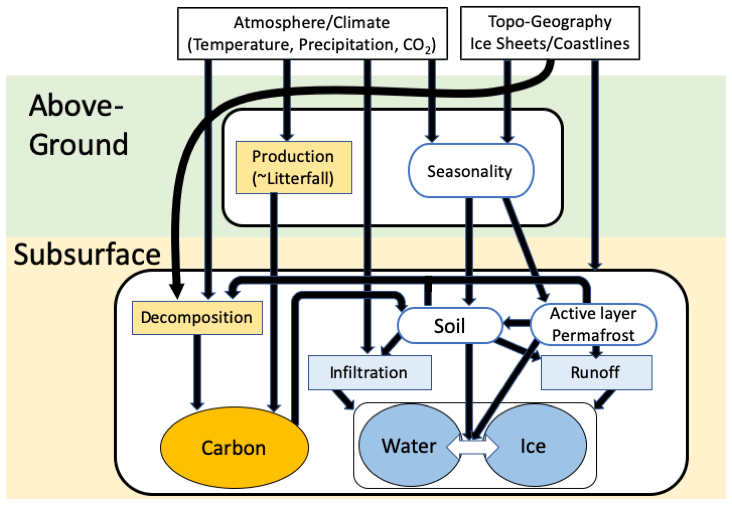
Figure 1 Schematic of the SOC-ICE-v1.0 numerical model to calculate soil organic carbon (SOC) and ground ice (ICE) budget.

2.2 Model description

The numerical soil organic carbon–ground ice budget model (SOC-ICE-v1.0) consists of two boxes: the “above-ground” box and the “subsurface” box (Fig. 1). The above-ground box is driven by mean annual air temperature (MAAT) and annual total precipitation (Precip) and has attributes such as latitude, longitude, altitude, distance from the closest ocean body, presence or absence of ice sheet cover, and background carbon dioxide concentration. The model diagnoses seasonality and frozen ground state and calculates the amount of carbon supply to the subsurface box. The subsurface box updates SOC, soil moisture, and ICE quantities, according to inputs passed from and climatic conditions determined by the above-ground box. The model was coded in Interactive Data Language (IDL; Harris Geospatial Solutions, Inc.). Sample model codes and associated data are provided as supplementary materials.

2.2.1 Above-ground processes

The above-ground box calculates (1) seasonality from local MAAT and its location information (continentality), and (2) the amount of carbon supply, as litter fall, to the subsurface box.

Seasonality and presence of frozen ground

As the reconstructed temperature data from the SeaRISE project, T_a, are obtained on an annual basis, they do not resolve the issue of seasonality, which is important in inferring the subsurface thermal state (i.e. presence of permafrost, seasonal freezing, or no freezing of ground) (Harris, 1981; Saito et al., 2014, 2016). We derived simple relationships between T_a and seasonal amplitude T_amp as a set of functions of location (longitude, latitude), distance from the coast of the closest ocean, and background climatic state, i.e. glacial (cold) or interglacial (warm) (Fig. 1 in the Supplement). For the warm period (defined in this study as 125 to 100 ka and after the Bølling–Allerød interstadial to the present day, judged by changes in reconstructed temperature and sea level data), the present-day climate was assumed to provide typical variations, and monthly data obtained from the ERA-Interim reanalysis were used. In contrast, monthly data obtained from the six PMIP3 models for the LGM simulations were used to derive average climatology for the cold periods (100 to 14 ka). The six models were selected to provide simulation results for both the LGM and the Holocene Climate Optimum (mid-Holocene run, 6 ka): CCSM4 (Gent et al., 2011), CNRM-CM5 (Voldoire et al., 2011), IPSL-CM5A-LR (Dufresne et al., 2013), MIROC-ESM (Watanabe et al., 2011), MPI-ESM-P (Brovkin et al., 2013), and MRI-CGCM3 (Yukimoto et al., 2012). Because the horizontal resolution and the sea–land mask differed between models, coastlines were determined for each model from its orography condition. Assuming the sinusoidal seasonal changes in temperature T_a+T_ampsin t, the freezing and thawing indices (FDD and TDD, respectively) were calculated as the cumulative degree day of the temperature below and above 0 ^∘C. The type of underlying frozen ground was then identified based on the classification method developed by Saito et al. (2014, 2016) as climate-driven permafrost (CP, corresponding to continuous permafrost), environmentally conditional permafrost (EP, corresponding to discontinuous permafrost), long-lasting seasonally frozen ground (Sf), intermittently frozen ground (If, frozen for a short duration, i.e. less than 2 weeks), or not frozen (Nf).

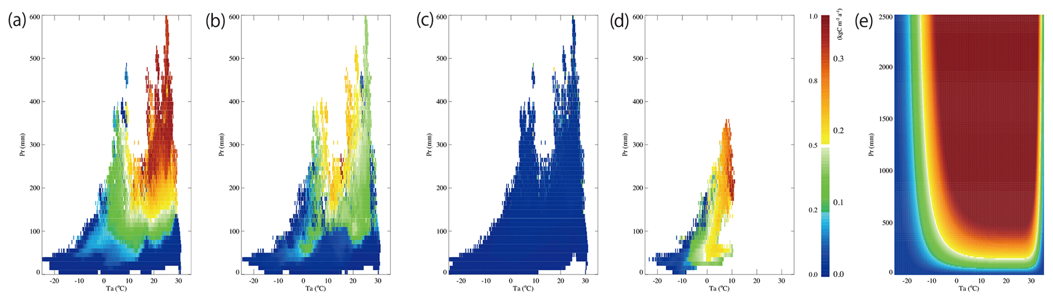
Figure 2 Distribution of litter fall, carbon input to the “subsurface” box, for a given mean annual air temperature (T_a) and annual total precipitation (Pr) pairs. (a) Distribution of litter fall outputs calculated by biogeochemical models and normalized to the respective maximum value: (a) VISIT, (b) Biome-BGC, (c) SEIB-N, and (d) CHANGE for global land areas, except for CHANGE, the result of which covered only land areas north of 50^∘ N. The scale is shown on the left-hand side of the colour bar. (e) The modelled litter fall distribution is based on simulated outputs for the functional shape and calibrated for absolute value by observation data. Note the vertical ranges are different for (e). The scale is shown on the right-hand side of the colour bar.

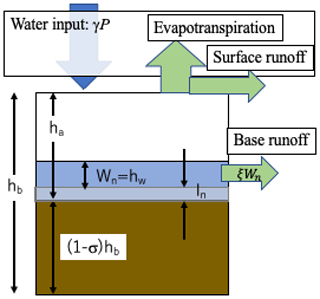
Figure 3 Schematic of hydrological processes of the subsurface box. It is a bucket-type reservoir of capacity h_b (m), consisting of liquid water (W_n=h_w) within the pore space (h_a=σh_b) and soil ((1−σ)h_b). Quantity of ice forming or melting at a time step is limited by current liquid or solid water amount, respectively (Eq. 9); total amount of ice (I_n) can supersede the capacity h_b to represent massive ground ice.

Table 1 List of parameters used in the model.

Litter fall

The amount of carbon supply to the subsurface box, calculated as litter fall (in $\mathrm{kg}\mathrm{C}{\mathrm{m}}^{-\mathrm{2}}{\mathrm{a}}^{-\mathrm{1}}$), was determined by the combination of MAAT T_a and total precipitation Pr (Fig. 3a.). For simplicity, we did not incorporate carbon type differences inherent in plant functional types (De Deyn et al., 2008). The shape of the litter fall function was determined by fitting the outputs of the biogeochemical models obtained from the GTMIP stage 2 project (Fig. 2a–d), i.e. VISIT (Ito, 2019), B-BGC (Thornton et al., 2002), SEIB-N (Sato et al., 2016), and CHANGE (Park et al., 2011). Relatively small values of SEIB-N, likely because of its biomass growth still being underway for this integration (see Fig. S3 in Pugh et al., 2020), did not change the resulting shape significantly. The derived function was then adjusted by multiplying it by a constant value to the best fit (in terms of least square errors) to the observational data: the compilation dataset of ecosystem functions in Asia (version 1.2). The resulting equation was formulated as follows:

$$\begin{array}{}\text{(1)}& \begin{array}{rl}\text{LitterFall}(T_{\mathrm{a}},\text{Pr},{\mathrm{CO}}_{\mathrm{2}})=& a_{\mathrm{1}}\left({\mathrm{CO}}_{\mathrm{2}}\right)\exp \left(-{\displaystyle \frac{(T_{\mathrm{a}}-T_{\mathrm{0}}{)}^{c_T}}{b_T}}\right)\\ & \cdot \log \left({\displaystyle \frac{\text{Pr}+P_{\mathrm{0}}}{b_P}}\right),\end{array}\end{array}$$

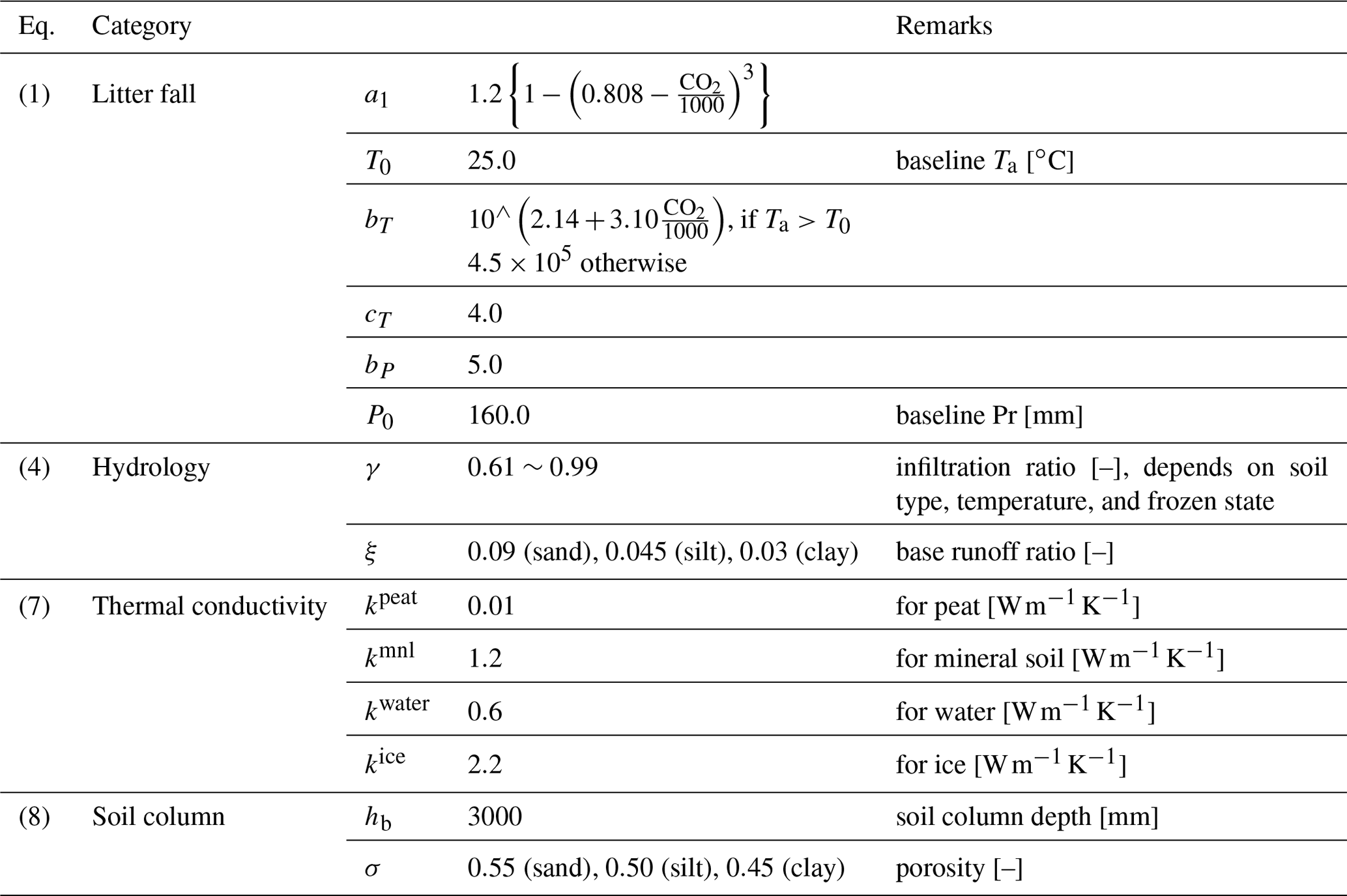
where T_a(t) and Pr(t) denote the values of MAAT and total precipitation, respectively, of the location in a year, t. T₀ and P₀ are the respective baseline values. a₁, b_T, c_T, and b_P are shape parameters. These parameters were determined by curve fitting to the model outputs (Fig. 2a–d) and observations; a₁ and b_T vary depending on the background atmospheric concentration of carbon dioxide CO₂ [ppm]. The values of these parameters and baseline values used in this study are summarized in Table 1. An example of the litter fall distribution under present-day climate conditions is shown in Fig. 2e.

2.2.2 Subsurface processes

The subsurface box has four major functions: (1) SOC budget, (2) water budget in the liquid phase, (3) assessment of freezing and thawing depths, and (4) phase change between ice and water. The box is not resolved for depth with explicit layering but an active area is assumed to be 3 m deep for hydrological calculations.

SOC budget

Accumulation and decay of organic carbon in the subsurface box are expressed as a difference equation, adopting Clymo's (1984) peat accumulation model for the catotelm. The change in SOC in the nth year, SOC_n, is formulated as Eq. (2).

$$\begin{array}{}\text{(2)}& {\displaystyle \frac{\mathrm{\Delta }{\text{SOC}}_n}{\mathrm{\Delta }t}}=\text{LitterFall}(T_{\mathrm{a}},\text{Pr},{\mathrm{CO}}_{\mathrm{2}})-{\mathit{\kappa }}_n\cdot {\text{SOC}}_{n-\mathrm{1}},\end{array}$$

where LitterFall [$\mathrm{kg}\mathrm{C}{\mathrm{m}}^{-\mathrm{2}}{\mathrm{a}}^{-\mathrm{1}}$] is the amount of organic carbon deposited on the ground as calculated using Eq. (1), and κ is the decomposition rate of SOC [a⁻¹], determined at each step by the following relaxation method:

$$\begin{array}{}\text{(3)}& {\mathit{\kappa }}_n={\mathit{\kappa }}_{n-\mathrm{1}}+{\displaystyle \frac{({\mathit{\kappa }}_{\text{crit},n}-{\mathit{\kappa }}_{n-\mathrm{1}})}{\mathit{\tau }}}\cdot \mathrm{\Delta }t.\end{array}$$

The critical equilibrium rate of decomposition, κ_crit,n, defined as SOC_n∕LitterFall_n, demonstrates that carbon supply from the above-ground box and the output (subsurface decomposition) of organic carbon are in balance under the given climate condition. Equation (3) suggests that the instant decomposition rate approaches the critical equilibrium value on the timescale defined by τ. This is the key parameter for the examination of climate and topo-geographic controls on soil carbon evolution, and we set the values of τ in this study in a geometric series at 4, 20, 100, and 500 years, adhering to considerations. Although closely related, τ does not represent the soil turnover (e.g. from tens to thousands of years; Perruchoud et al., 1999; Conant et al., 2011; Luo et al., 2019) or ecological secondary succession (e.g. from a few years to tens of years following wildfire in permafrost areas; Yohikawa et al., 2002; Narita et al., 2015; or from tens to hundreds of years under temperate conditions; Svenning and Sandel, 2013). It is a hypothetical variable representing the timescale for decomposition to approach its equilibrium value under the given climate and topo-geographic condition. For peatlands in the taiga and tundra that lie between sub-Arctic and Arctic regions, it may take more than a thousand years to reach an equilibrium, due to the slow plant growth and carbon decomposition because of the cool and/or dry environment, whereas it can happen on a yearly order, O(1 year), in warm and moist tropical rainforests, where the fast cycle of vegetation growth/death and decomposition facilitates rapid changes (Harden et al., 1992; Vitt et al., 2000b). We also incorporated impacts of permafrost presence and wetness of the ground on SOC dynamics by specifying a larger value of τ, determined according to frozen and/or wet conditions (e.g. 2500 years for saturated frozen ground in continuous permafrost zones and 1500 years for saturated frozen ground in discontinuous permafrost zones).

Hydrological process

Figure 3 shows a schematic of the subsurface hydrological model for exposed land (i.e. not covered by ice sheet or water). The budget of the liquid-phase water W_n is controlled using Eq. (4) as the balance between the input (the first term on the right-hand side) and the output (the second and third terms).

$$\begin{array}{}\text{(4)}& {\displaystyle \frac{\mathrm{\Delta }{W}_n}{\mathrm{\Delta }t}}=\mathit{\gamma }\text{Pr}-\mathit{\xi }{W}_{n-\mathrm{1}}-{\mathit{\phi }}_n\end{array}$$

The first term in Eq. (4) refers to annual net precipitation (i.e. precipitation – evapotranspiration – surface runoff), with γ denoting the ratio of subsurface infiltration to the total precipitation. The second term refers to base runoff as a function of water storage in the liquid phase, and ξ is a parameter for the ratio of base runoff. The third term refers to new ice freezing or melting at a time step. Soil moisture [mm] in the active area overflows as runoff when it exceeds the saturation soil moisture (h_a=σh_b), where σ is porosity, and h_b is the depth of the hydrologically active area set to 3000 mm in this study (Fig. 3). In contrast, the overall storage of ICE at location I_n has no limitation (to mimic the development of ice wedge) and is updated using Eq. (5). The computation of φ is described in the next subsection.

$$\begin{array}{}\text{(5)}& I_n={\mathit{\phi }}_n+I_{n-\mathrm{1}}\end{array}$$

The parameters of soil characteristics (porosity σ, infiltration rate γ, and base runoff ratio ξ of the area) are summarized in Table 1.

Assessment of freezing and thawing depths

The changes in the amount of ICE, φ_n, are analysed by identifying the energy balance between ground freezing and thawing processes. They are set proportional to the depth of freezing $d_n^{\mathrm{f}}$ and thawing $d_n^{\mathrm{t}}$, which are empirically determined by Eq. (6a–b) from ground thermal conductivity (for the frozen state, $k_n^{\mathrm{f}}$, and thawed state, $k_n^{\mathrm{t}}$, respectively) and respective freezing and thawing indices calculated in the above-ground box (i.e. FDD and TDD).

$$\begin{array}{}\text{(6a)}& {\displaystyle }& {\displaystyle }{d}_n^{\mathrm{f}}=\sqrt{{\displaystyle \frac{\mathrm{2}{k}_n^{\mathrm{t}}\cdot \text{FDD}}{W_n/h_{\mathrm{b}}{\mathit{\rho }}_{\mathrm{w}}\cdot \mathit{\lambda }}}}={\mathit{\alpha }}_f\sqrt{\text{FDD}},\text{(6b)}& {\displaystyle }& {\displaystyle }{d}_n^{\mathrm{t}}=\sqrt{{\displaystyle \frac{\mathrm{2}{k}_n^{\mathrm{f}}\cdot \text{TDD}}{W_n/h_{\mathrm{b}}{\mathit{\rho }}_{\mathrm{w}}\cdot \mathit{\lambda }}}}={\mathit{\alpha }}_t\sqrt{\text{TDD}},\end{array}$$

where ρ_w is the density of water, and λ is the latent heat of fusion. Thermal conductivity is evaluated from carbon and water content using Eq. (7).

$$\begin{array}{}\text{(7)}& \begin{array}{rl}& k_n^{\mathrm{t},\text{dry}}={\displaystyle \frac{{\text{SOC}}_n}{{\mathit{\chi }}^{\mathrm{t},\text{dry}}}}{k}^{\text{peat}}+\left(\mathrm{1}-{\displaystyle \frac{{\text{SOC}}_n}{{\mathit{\chi }}^{\mathrm{t},\text{dry}}}}\right)k^{\text{mnl}}\\ & k_n^{\mathrm{t}}={\displaystyle \frac{W_n}{{\mathit{\chi }}^{\mathrm{t},\text{wet}}}}{k}^{\text{water}}+\left(\mathrm{1}-{\displaystyle \frac{W_n}{{\mathit{\chi }}^{\mathrm{t},\text{wet}}}}\right)k_n^{\mathrm{t},\text{dry}}\\ & k_n^{\mathrm{f}}={\displaystyle \frac{I_n}{{\mathit{\chi }}^{\mathrm{f}}}}{k}^{\text{ice}}+\left(\mathrm{1}-{\displaystyle \frac{I_n}{{\mathit{\chi }}^{\mathrm{f}}}}\right)k_n^{\mathrm{t}},\end{array}\end{array}$$

where k^peat, k^mnl, k^water, and k^ice denote thermal conductivity values for carbon-containing and mineral parts of the soil, water, and ice, respectively. The relative amounts of thawed dry or wet soil and frozen soil are defined by Eq. (8).

$$\begin{array}{}\text{(8)}& \begin{array}{rl}{\mathit{\chi }}^{\mathrm{t},\text{dry}}({\text{SOC}}_n,h_{\mathrm{b}};\mathit{\sigma })=& (\mathrm{1}-\mathit{\sigma })h_{\mathrm{b}}+{\text{SOC}}_n\\ {\mathit{\chi }}^{\mathrm{t},\text{wet}}(W_n,{\text{SOC}}_n,h_{\mathrm{b}};\mathit{\sigma })=& (\mathrm{1}-\mathit{\sigma })h_{\mathrm{b}}+{\text{SOC}}_n+W_n\\ =& {\mathit{\chi }}^{\mathrm{t},\text{dry}}+W_n\\ {\mathit{\chi }}^{\mathrm{f}}(I_n,{\text{SOC}}_n,h_{\mathrm{b}};\mathit{\sigma })=& (\mathrm{1}-\mathit{\sigma })h_{\mathrm{b}}+{\text{SOC}}_n+I_n\\ =& {\mathit{\chi }}^{\mathrm{t},\text{dry}}+I_n\end{array}\end{array}$$

Phase change between water and ice

The change in the amount of ice is calculated as follows:

$$\begin{array}{}\text{(9)}& \mathit{\phi }=\left\{\begin{array}{l}-I_n\\ \stackrel{\mathrm{̃}}{\mathit{\phi }}\\ W_n\end{array}\right.\text{if}\stackrel{\mathrm{̃}}{\mathit{\phi }}:\left\{\begin{array}{l}\cdot <-I_n\\ -I_n\le \cdot \le W_n,\\ W_n<\cdot ,\end{array}\right.\end{array}$$

where $\stackrel{\mathrm{̃}}{\mathit{\phi }}$ is expressed as

$$\begin{array}{}\text{(10)}& \stackrel{\mathrm{̃}}{\mathit{\phi }}=\mathit{\beta }\left(d_n^{\mathrm{f}}-d_n^{\mathrm{t}}\right){\displaystyle \frac{W_n}{h_{\mathrm{b}}}}.\end{array}$$

β is a parameter that controls the distribution of energy in melting or freezing of water, β_freeze=0.5; β_thaw=1.0. The parameter values not listed here are summarized in Table 1.

2.3 Driving and boundary condition data

The model is driven by inputs of MAAT, Pr, and atmospheric carbon dioxide concentration, along with geographical information: longitude, latitude, continentality, and land condition types (i.e. exposed land, under water, or under ice sheets). In this study, the model was integrated for the last 125 kyr north of 50^∘ N in the Northern Hemisphere with 1^∘ resolution, aligning with the grid system of the employed dataset for ice sheet evolution (i.e. ICE-6G_C).

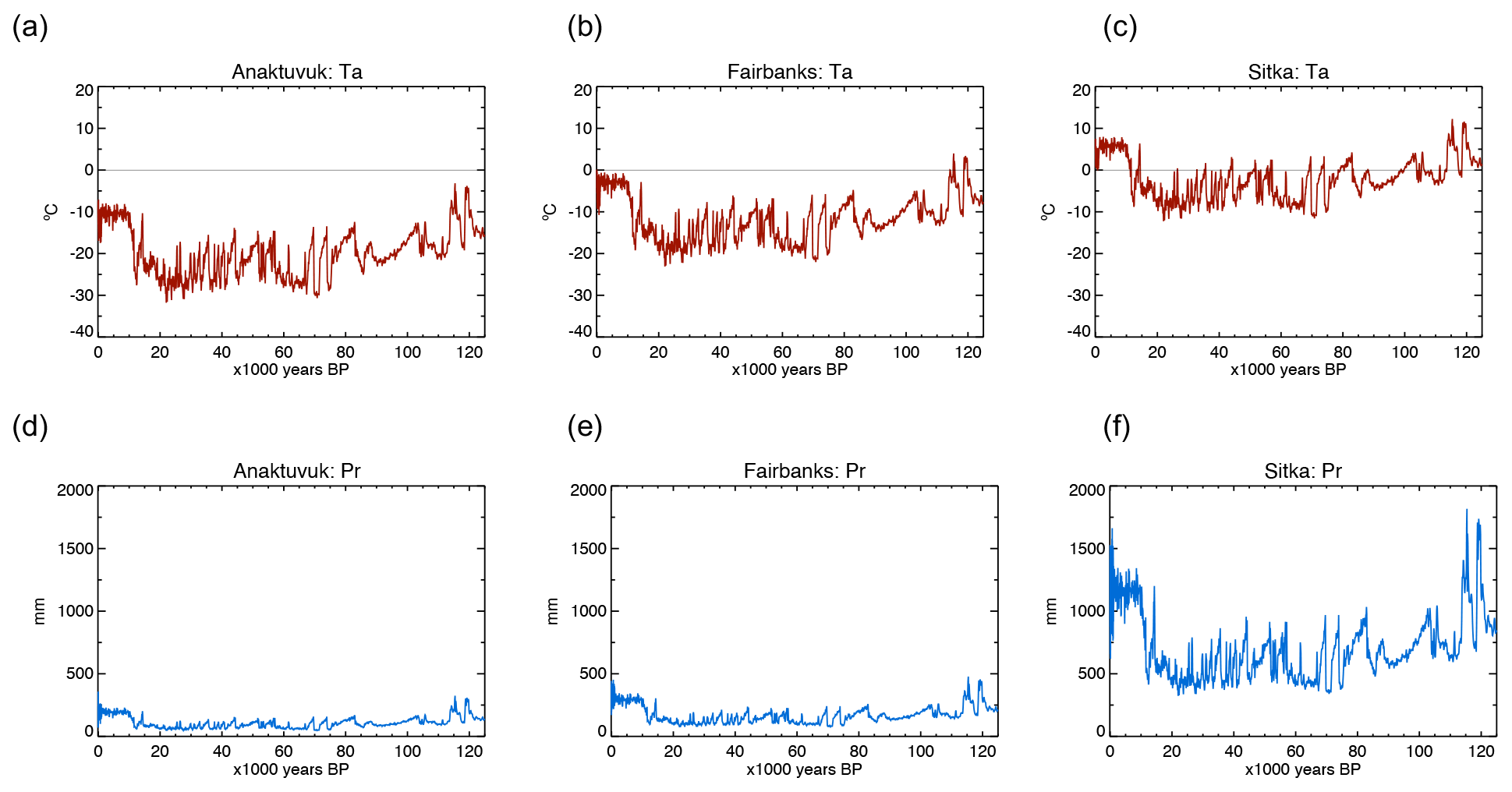
Figure 4 Example time series of climate forcing data (temperature, precipitation). The temporal variations in climate forcing data were reconstructed from Greenland ice core data (the SeaRISE project), while present-day climatology at the 1^∘ grid point was derived and interpolated from ERA-Interim reanalysis. Mean annual air temperature (T_a; in ^∘C) at the Alaskan grid point closest to (a) Anaktuvuk (69.5^∘ N), (b) Fairbanks (64.5^∘ N), and (c) Sitka (57.5^∘ N). Panels (d–f) are the same as panels (a–c) except for annual total precipitation (Pr; in mm).

2.3.1 Forcing data for 125 kyr

The baseline 125 kyr time series of annual temperature and precipitation was obtained from the SeaRISE project (Bindshadler et al., 2013). The time series presents deviations from current mean temperature or ratios to the current precipitation amount. The SeaRISE time series requires present-day climatology data for a specific location. The present-day climatology was computed from ERA-Interim reanalysis data for the years 1979–2016. Moreover, the SeaRISE time series has low temporal resolution in the recent millennium (i.e. 100-year intervals). We examined the SOC time series calculated using the forcing data obtained from the CMIP5/PMIP3 models for the period (the last millennium and the historical runs), with respect to the mean values, temporal variability, and smooth connectivity to the historical period, to select the IPSL simulation results. The SeaRISE data for the period 850–1850 were replaced by the outputs from its “last millennium” run and that for the period 1850–1900 by its “historical” run. Similarly, the anomaly time series for the period 1900–2006 was constructed using the University of Delaware reconstruction product (UDel_AirT_Precip).

Considering the meridional dependence (i.e. polar amplification effect) of δT_a, the amplitude of temperature variations between glacial and interglacial periods and the amplitude of the SeaRISE anomaly temperature time series were reduced southward within the 50 and 70 meridional bands at a rate of 0.25 ^∘C per 1^∘ resolution from its original value, 23.3 ^∘C, which was determined by preliminary analysis on [$\partial \left(\mathit{\delta }{T}_{\mathrm{a}}\right)/\partial \text{lat}$] for six PMIP3 models (Fig. 2 in the Supplement). These time series were then combined with present-day climatology to produce a 125 kyr time series for each 1^∘ resolution grid point. Examples of the reconstructed time series of temperature and precipitation for three different locations in Alaska are shown in Fig. 4.

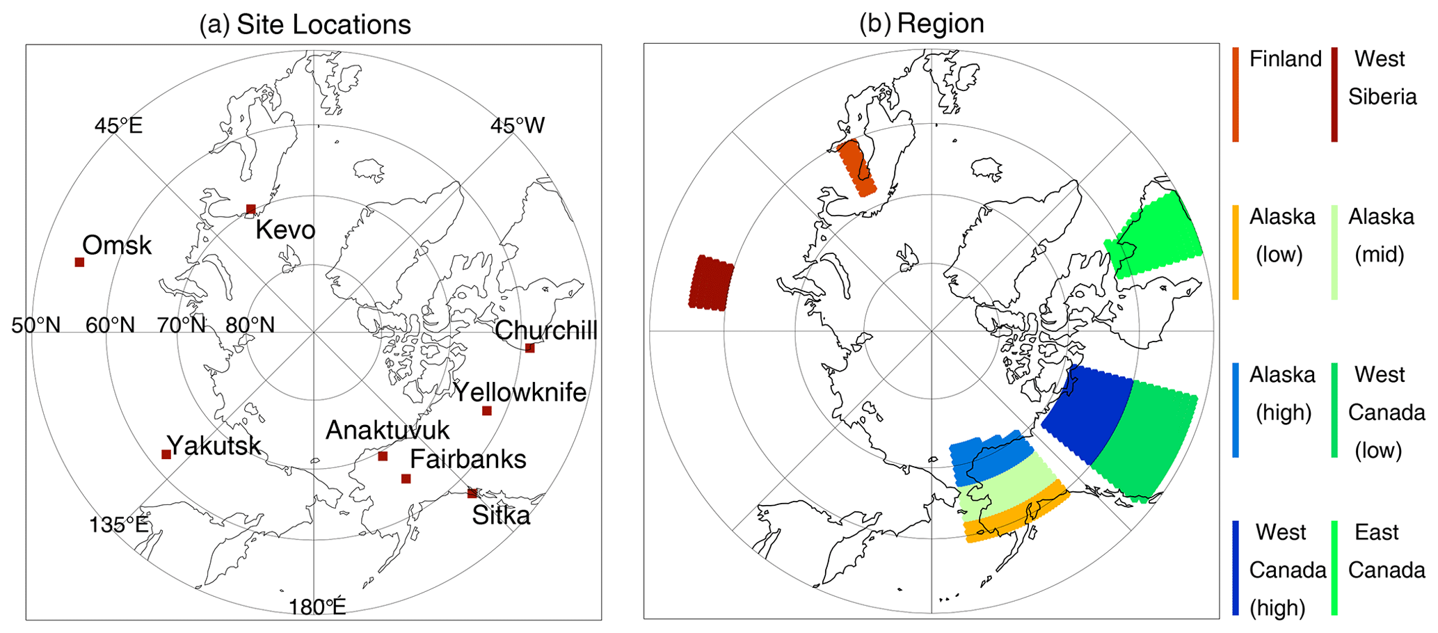
Figure 5 (a) Locations of the eight sample sites for comparison of simulated time series. (b) Areal extents of the eight subregions for analysis of the accumulation history of SOC and ICE.

2.3.2 Boundary conditions

For the last 125 kyr of the integration period, there have been substantial changes in the presence and thickness of ice sheets, as well as in altitudes and coastlines, in the circum-Arctic area. These surface boundary conditions significantly affect the calculation of subsurface carbon and ice dynamics through various processes such as submergence, uplift, burial under ice sheets, and removal by glacial dynamics. We used the ICE-6G_C datasets (Argus et al., 2014; Peltier et al., 2015) to determine altitude, the areal ratio of land, water, and ice cover, and ice thickness for the original 1^∘ grid points. Each grid point has three sections, i.e. exposed land, under ice, and under water (e.g. sea, lake), following the areal fraction of land and ice of the dataset. The amounts of carbon, ice, and water are reshuffled due to changes in land cover fractions, in addition to the internal dynamics of carbon and water determined by Eqs. (2) and (4). When some portion of the grid submerges, the SOC amount and ice content, as well as frozen ground condition, belonging to this areal portion remain unchanged but the water content to the portion becomes saturated. Similarly, SOC and ICE remain unchanged under ice sheets except when some portion of the grid becomes ice-free (melting of ice sheet). In such cases, water from the melting ice is added to the precipitation input (in Eq. 4) and the SOC amount corresponding to the newly exposed areal fraction is lost from the grid's storage to reflect basal ablation.

2.3.3 Initial values and spin-up

We examined the model's sensitivity to initial values with a small set of different SOC (namely, 5.0, 10.0, 20.0, 22.5, 25.0, 27.5, 30.0, 50.0, and 100.0 kg C m⁻²) and soil moisture (100, 500, 1000, and 1500 mm for the 3000 mm column) values in limited locations (see Fig. 5a). The model sensitivity showed clear dependency on the initial values of SOC but was negligible for soil moisture. Based on this preliminary examination, we determined the initial values that would produce the most realistic range for the present-day circum-Arctic, namely 25.0 kg C m⁻² for SOC and 500 mm for soil moisture.

Before full integration, the model was spun up (or equilibrated) for a certain period of years to attain an internal balance in the SOC, soil moisture, and ICE budget with the forcing. We integrated the model for 5000 years for spin-up with the constant forcing and perpetual boundary data taken from the 125 ka condition, starting from the uniform initial values of 25.0 kg C m⁻² of SOC and 500 mm of soil moisture at all grid points to reach an equilibrated state.

Table 2 Comparison of simulated SOC and ICE with observation-based data for eight locations. Longitude, latitude, the climatology of mean annual air temperature (T_a) and annual total precipitation (Pr), and the simulated results are obtained from the values of the nearest 1^∘ resolution grid point. τ denotes the relaxation timescale of decomposition rate.

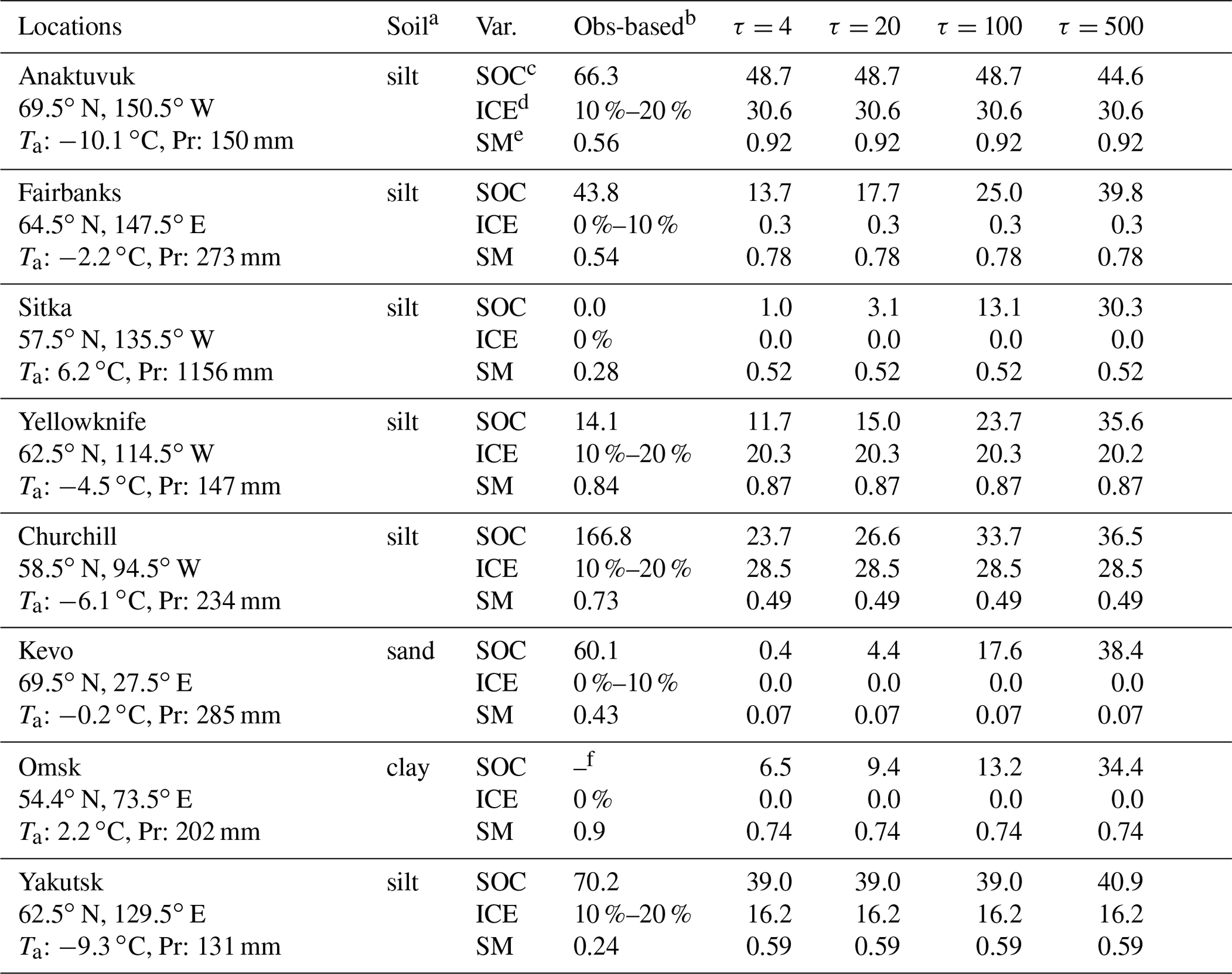
Climatology of temperature (T_a) and precipitation (Pr) is the average of the driving data for the period 1981–2010.
^a Soil types are determined from the “basic soils information” used for the 1^∘ resolution in the GLDAS (Rodell et al., 2004) dataset (https://ldas.gsfc.nasa.gov/gldas/soils (last access: 25 January 2021). ^b Soil organic carbon amount is obtained from Olefeldt et al. (2016); ground ice content category is obtained from Brown et al. (1998). In both cases, the values of the nearest grid point were used. ^c Observation-based and simulated soil organic carbon is in kg C m⁻². ^d Ground ice is shown in categorical volumetric percentage for the observation-based quantity, while simulated values are shown in terms of ice thickness in metre. ^e Soil moisture in terms of saturation ratio was calculated, respectively, from the GLDAS Mosaic product (assimilated data) and the SOC-ICE-v1.0 results, assuming the same porosity. ^f No data were found in the vicinity.

2.3.4 Locations for model examinations

The behaviour of the model was evaluated in terms of the simulated 125 kyr time series for selected locations and the regional characteristics for different circum-Arctic regions.

The simulated time series of the SOC, ICE, and soil moisture were examined at the selected eight locations with different climatic characteristics for the 125 kyr period. The locations denote the grid points closest to each specified site shown in Fig. 5a. Of these, three sites are in Alaska: Anaktuvuk on the North Slope (continuous permafrost, Jones et al., 2009; Hu et al., 2015; Iwahana et al., 2016), Fairbanks in interior Alaska (discontinuous permafrost, Miyazaki et al., 2015; Sueyoshi et al., 2016), and Sitka in southeast Alaska on the Pacific coast (seasonally frozen ground). Sitka is the warmest and most pluvial site of the eight. Two sites are in Canada: Yellowknife by the Great Slave Lake in the Northwest Territories (discontinuous permafrost) and Churchill in Hudson Bay Lowlands (continuous permafrost, Dyke and Sladen, 2010; Sannel and Kuhry, 2011). Both of these were under the Laurentide Ice Sheet during the last glacial period and started carbon accumulation after deglaciation at different times (Dyke, 2005). Three sites are in Eurasia. Kevo in northern Finland (Miyazaki et al., 2015; Sueyoshi et al., 2016), which was covered by the Fennoscandia Ice Sheet during the last glacial period, has oceanic influence and is located in the discontinuous permafrost zone. Omsk in southwestern Siberia (seasonally frozen ground) has continental characteristics and has been ice-free. Yakutsk is in East Siberia (continuous permafrost; Miyazaki et al., 2015; Sueyoshi et al., 2016). Anaktuvuk and Yakutsk are obtained from areas where the ice-rich permafrost can be found (Kanevsky et al., 2011; Murton et al., 2015). Geographical and climatological data of these locations are shown in the two leftmost columns in Table 2.

Further, we specified eight circum-Arctic regions to compare the simulated carbon and ice dynamics with values reported in the literature (Smith et al., 2004; McDonald et al., 2006; Yu et al., 2009; Jones and Yu, 2010). The locations and areas of these eight regions are as follows: Alaska (high latitudes) (67.5–73.5^∘ N, 169.5–139.5^∘ W), Alaska (middle latitudes) (62.5–67.5^∘ N, 169.5–139.5^∘ W), Alaska (low latitudes) (59.5–62.5^∘ N, 169.5–139.5^∘ W), western Canada (high latitudes) (60.5–69.5^∘ N, 129.5–103.5^∘ W), western Canada (low latitudes) (51.5–60.5^∘ N, 129.5–103.5^∘ W), eastern Canada (44.5–62.5^∘ N, 73.5–59.5^∘ W), Finland (60.5–68.5^∘ N, 22.5–27.5^∘ E), and West Siberia (55.5–60.5^∘ N, 72.5–84.5^∘ E) (Fig. 5b).

3 Results and discussions

The amounts of SOC, ICE, and soil moisture were computed using the SOC-ICE-v1.0 model. The calculation was performed on the 1^∘ interval grid system. Here, we have examined the simulated time series for SOC, ICE, and soil moisture through the glacial and interglacial periods in the circum-Arctic regions and have discussed the behaviour of the model.

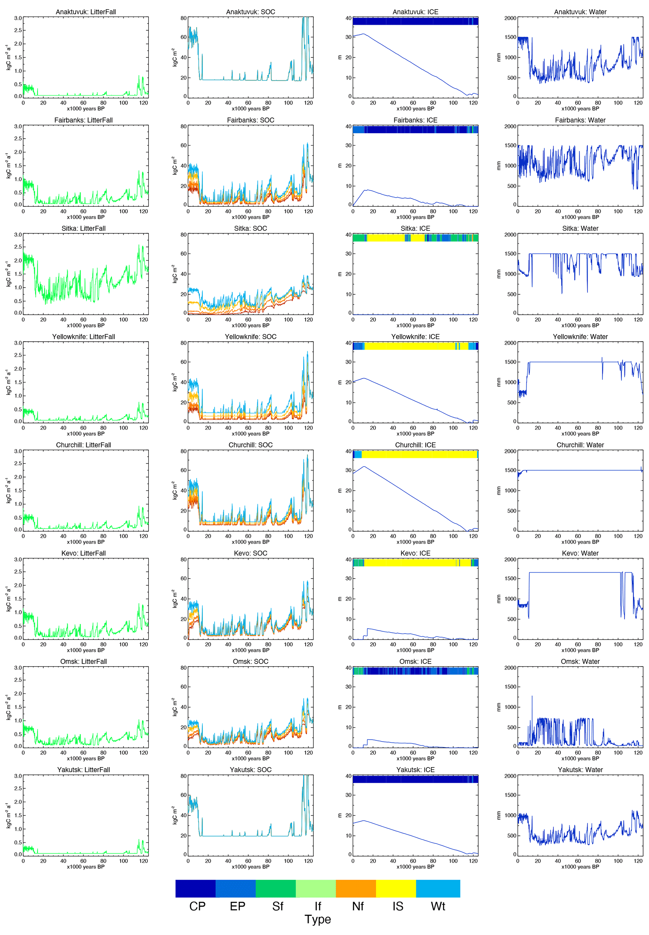
Figure 6 Results of model simulations for the eight circum-Arctic sites shown in Fig. 5. The 125 kyr time series of litter fall (in kg C m⁻²; leftmost column), SOC (in kg C m⁻²; second from left), ICE (in metres; second from right), and groundwater in liquid phase (water in mm; rightmost column) are shown for different values of τ, relaxation timescale of decomposition rate (red: 4 years, orange: 20 years, yellow: 100 years, blue; 500 years). The legend shows land cover types for continuous permafrost (CP, deep blue), discontinuous permafrost (EP, blue), seasonally freezing ground (Sf, green), intermittently frozen ground (If, pale green), no freezing (Nf, orange), ice sheets (IS, yellow), and water body (Wt, pale blue).

3.1 Time series analysis

Table 2 shows the results of the simulated present-day content and corresponding observation-based data at the eight selected locations with respect to SOC, ICE, and soil moisture (relative to the saturation level). In Table 2, the calculated SOC content with different values of τ is compared with O16 total SOC amount at the nearest point. The computed ICE content was compared with IPA-ICE. The larger the value of τ, the larger the simulated SOC amount for the present day. On the contrary, ICE content showed almost no sensitivity to τ under current formulae (Eqs. 4–10). The resulting ranges at eight locations and intersite variations in the simulated present-day SOC and ICE content were largely consistent with observation-based data, except for underestimation of SOC and overestimation of ICE at the Churchill site. Moreover, the value of τ has a discernible control over the simulated present-day SOC amount for all locations except Anaktuvuk and Yakutsk, which have almost entirely been in continuous permafrost zones throughout the integration period (Fig. 6).

3.1.1 Soil organic carbon

Figure 6 shows the 125 kyr time series of model outputs for litter fall, SOC, ICE, and soil moisture at eight locations. Litter fall (the leftmost column in Fig. 6) increased proportionally to annual temperature and precipitation (Eq. 1, Figs. 2a and 4). Although the values of litter fall appeared to be larger than observed values, the resulting SOC amount and its circum-Arctic distribution did not show overestimation (see the SOC column of Fig. 6; cf. Saito et al., 2020). This result is discussed in Sect. 3.3.2, along with suggestions for future improvements. The simulated SOC changes showed a tendency for accumulation to be active during warm (i.e. interglacial) periods and inactive during cold (i.e. glacial) periods at all locations. This is consistent with existing knowledge (Vitt et al., 2000a, b; Charman et al., 2015).

The carbon accumulation time series shows high sensitivity to τ, except in continuous permafrost zones, in line with the result of dependency of present-day SOC amounts on τ (Table 2). These behaviours demonstrated adequate functionality of τ to represent allogenic controls of external (i.e. climatic, topographic and/or land composition) conditions over carbon dynamics in terms of the time required to shift to equilibrium under meandering climate conditions (Belyea and Baird, 2006; Loisel et al., 2017).

3.1.2 Ground ice

Accumulation of ICE during the glacial period and its decrement after the onset of deglaciation were observed at all locations except for Sitka, where no ICE was accumulated throughout the period. In continuous permafrost zones with no ice sheet coverage, i.e. in Anaktuvuk and Yakutsk, ICE steadily accumulated during glacial periods and persists to date, despite some melting in the Holocene. For sites entirely covered with land ice during the glacial period, e.g. Yellowknife, Churchill, and Kevo, ICE accumulated even under land ice. This can be interpreted as the potential amount of buried massive ice at those locations but may require further consideration and/or modifications in model formulations. Moreover, the absolute values of simulated ICE do not necessarily show the in situ amount found in the soil layer. Rather, they indicate a relative value to be compared among different locations for contemporary spatial variations or temporal development.

3.1.3 Soil moisture

Temporal changes in soil moisture (in liquid phase) are presented in the rightmost column of Fig. 6. In (continuous) permafrost zones, this value should be interpreted as the amount of liquid water available in summer, not the total amount of liquid water kept unfrozen during winter or over the entire period. Despite the difficulty in examining the likeliness of simulated long-term changes and intersite differences in quantitative comparisons with observation-based evidence due to lack of data, qualitative behaviour can be interpreted. The water level after deglaciation depended largely on precipitation amount and frozen ground type (e.g. continuous, discontinuous permafrost, or seasonally frozen ground). At the Anaktuvuk and Yakutsk sites, which were underlain by cold continuous permafrost, the ground was dry during the glacial period and wet in the warmer Holocene because the length of the thawing period and depth of the thawed layer were limited under glacial conditions, with most liquid water frozen and stored as ice, while the active layer was thicker and persisted longer during the Holocene. In a warmer continental location, like Omsk, the water content was higher when underlain by permafrost than when ice-free, to which the decrease in base runoff and evapotranspiration may likely contribute. In Fairbanks, which is also an interior location but cooler and wetter than Omsk, the average and range of temporal variations remained unchanged for the entire integration period. Greater availability of water due to a wetter climate may have contributed to larger fluctuations during the Holocene than in the Omsk case. At those locations covered under land ice during the glacial period (e.g. Sitka, Yellowknife, Churchill, and Kevo in Fig. 6), soil moisture was saturated under ice sheets (n.b., by formulation) but commonly became drier once the ice sheets retreated.

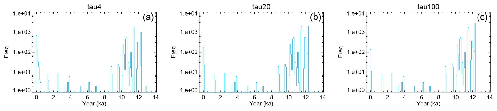
Figure 7 Histograms of circum-Arctic basal age distribution of the SOC accumulation for different values of τ: (a) 4 years, (b) 20 years, and (c) 100 years. The ordinate (frequencies) is in the logarithmic scale.

3.2 Regional analysis for the deglaciation period

We also examined the regional characteristics related to the carbon and ground ice dynamics for the eight circum-Arctic regions (Fig. 5b), i.e. basal age distribution (Sect. 3.2.1) and accumulation rates (Sect. 3.2.2) for the post-glacial SOC accumulation, and the post-glacial ICE accumulation and dissipation (Sect. 3.2.3).

3.2.1 Basal age of carbon accumulation

Figure 7a–c show histograms of the basal age of post-glacial soil carbon accumulation over the entire circum-Arctic domain (north of 50^∘ N). The simulated results showed a peak of northern high-latitude SOC initiation during the 12–10 ka period, with the unequivocal concentration of the peak (logarithmic vertical scale in Fig. 7). This is consistent with the observational studies that showed a gentler distribution of initiation after the LGM at 11–9 ka, although shifted later by a millennium and with regional differences (Smith et al., 2004; McDonald et al., 2006; Yu et al., 2009, 2010; Jones and Yu, 2010; Loisel et al., 2017; Morris et al., 2018). There may be multiple reasons for this discrepancy. One possibility is related to the forcing data. Local climatic history varied according to the location (Morris et al., 2018), while climate data reconstructed from a Greenland ice core were in phase at all locations (Fig. 4a–c) except for the differences in timings of ice sheet retreat or submergence. Another possibility is insufficiency in the parameterization of carbon input (Eq. 1) and output (Eqs. 2–3). The discrepancy may also be attributed to differences or technical limitations in the determination of SOC initiation. For numerical data, the basal age can be defined precisely as the first time step with non-zero accumulation of SOC after the LGM. The limit of detection in the laboratory may simply not work at the same detection level. Despite these limitations, the results capture the impacts of external climatic changes (i.e. an allogenic control) on carbon dynamics during the deglaciation period.

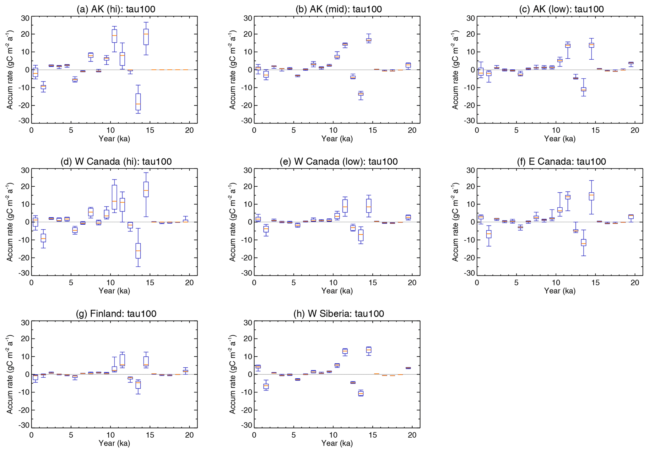
Figure 8 Millennial changes in the carbon accumulation rate ($\mathrm{g}\mathrm{C}{\mathrm{m}}^{-\mathrm{2}}{\mathrm{a}}^{-\mathrm{1}}$) after the LGM for different circum-Arctic regions: (a) high Alaska, (b) mid-Alaska, (c) low Alaska, (d) high western Canada, (e) low western Canada, (f) eastern Canada, (g) Finland, and (h) West Siberia. The statistical distribution of the accumulation rates, aggregated for each region for each millennial period, is illustrated by a box–whisker plot. The lowest and highest whiskers of the box–whisker plots show the 10th and 90th percentiles, respectively. The lower and upper edges of the box show the 25th and 75th percentiles, respectively. The 50th percentile (median) is shown by the coloured bar in the box. Areas of each region are shown in Fig. 5b.

3.2.2 SOC accumulation rates

Figure 8 shows temporal changes in the post-glacial SOC accumulation rate for eight regions (Fig. 5b). Accumulation rates were calculated from the original simulated annual time series, aggregated for regions for every millennial interval. The general tendencies were reasonably reproduced such that the accumulation rate was high at 12–9 ka and in the last millennium, while it was low to modest in between (cf. Plates 3b and 5d in Yu et al., 2009, Figs. 1c and 3 in Yu, 2012). Yu et al. (2009) reported the observation-based estimates of topical and local accumulation rates in different circum-Arctic regions in the Holocene: 24.1 $\mathrm{g}\mathrm{C}{\mathrm{m}}^{-\mathrm{2}}{\mathrm{a}}^{-\mathrm{1}}$ in Fairbanks, Alaska (middle latitude), 5.7–13.1 $\mathrm{g}\mathrm{C}{\mathrm{m}}^{-\mathrm{2}}{\mathrm{a}}^{-\mathrm{1}}$ in Alaska (low latitude), 15.6–31.7 $\mathrm{g}\mathrm{C}{\mathrm{m}}^{-\mathrm{2}}{\mathrm{a}}^{-\mathrm{1}}$ in western Canada (low latitude), 7.0–30.6 $\mathrm{g}\mathrm{C}{\mathrm{m}}^{-\mathrm{2}}{\mathrm{a}}^{-\mathrm{1}}$ in eastern Canada, 12.9–22.5 $\mathrm{g}\mathrm{C}{\mathrm{m}}^{-\mathrm{2}}{\mathrm{a}}^{-\mathrm{1}}$ in Finland, and 21.9–70.6 in West Siberia. The simulated results in Fig. 8 are reasonably consistent with the field-based values; however, it also shows the need for improvement.

Simulated accumulation rates can show negative values (corresponding to dissipation or decomposition of stored carbon and the possible release to the atmosphere in gaseous phase). On the contrary, only positive estimates can be reconstructed from excavated cores. Studies show that initiation peaks for northern peatlands occur at approximately 11–9 ka (Yu et al., 2010), and the reported basal ages of the core samples from those regions are rarely earlier than 13 ka (Smith et al., 2004; MacDonald et al., 2006; Morris et al., 2018). The large negative values implying extensive decomposition at approximately 13–12 ka are consistent with available information and thus are worth further investigation.

Figure 9 Same as Fig. 8, except for ground ice accumulation in mm a⁻¹.

3.2.3 Changes in ground ice

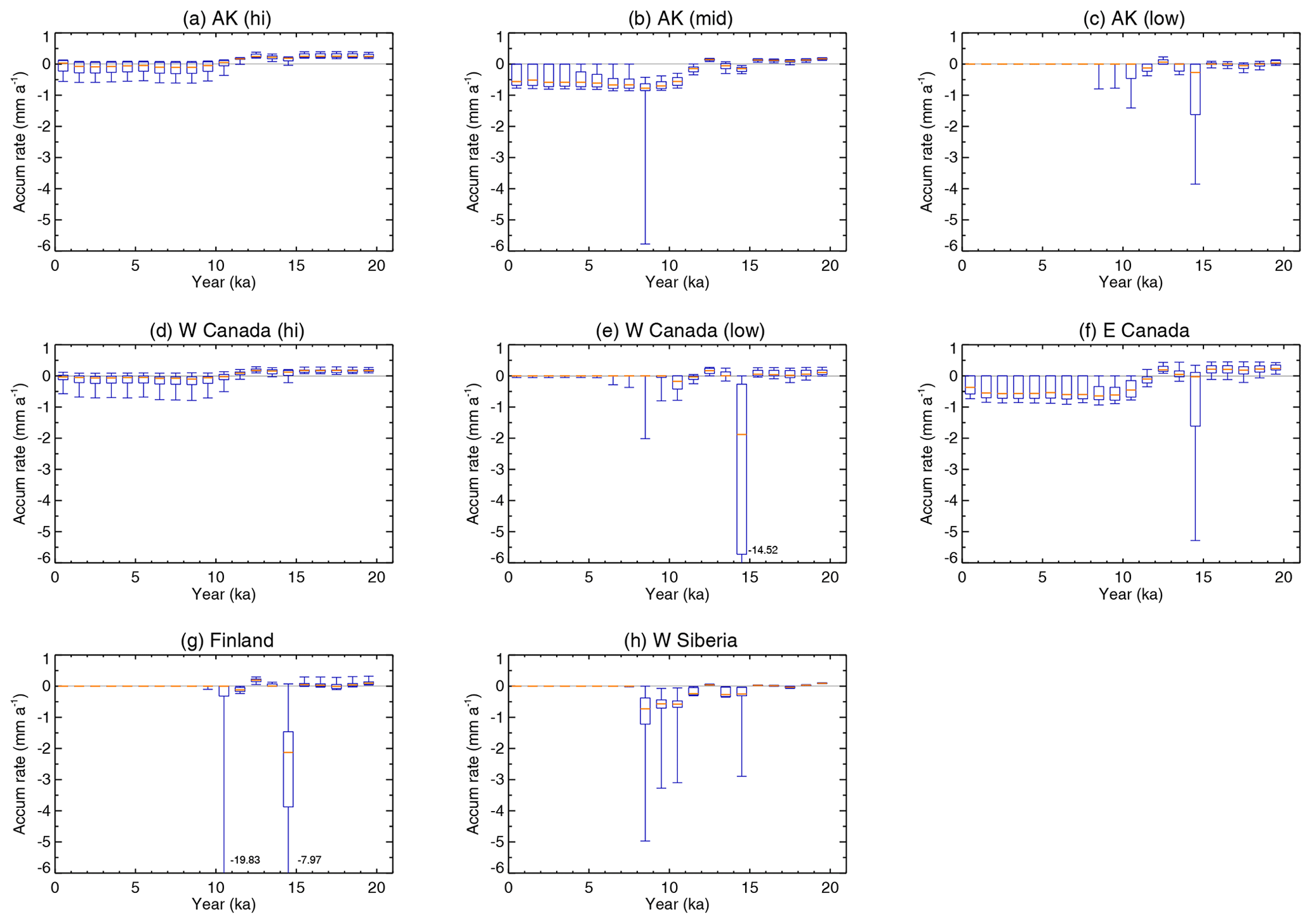
Similar plots for temporal changes in the regional budget of ICE after the LGM are shown in Fig. 9. In all eight regions, general accumulation of ground ice was simulated until the end of 15 ka. During the 15–14 ka period, large melting of ground ice occurred in relatively warmer areas, i.e. western Canada (low), eastern Canada, Finland, and West Siberia. The melting occurred at 11–9 ka but at a lower rate. These apparent synchronous melting in these areas at 15–14 ka likely resulted from the single-sourced warming peak of the Bølling–Allerød interstadial in the SeaRISE time series (e.g. Fig. 4a–c) and suggests the need for further studies to include local climate variations to the driving data. Ground ice accumulation continued after 12 ka only in colder regions, such as high-latitude areas in Alaska and western Canada. These regional differences in and characteristics of simulated ICE evolution suitably correspond to current conditions; however, the validation of these temporal changes using observation-based sources is difficult.

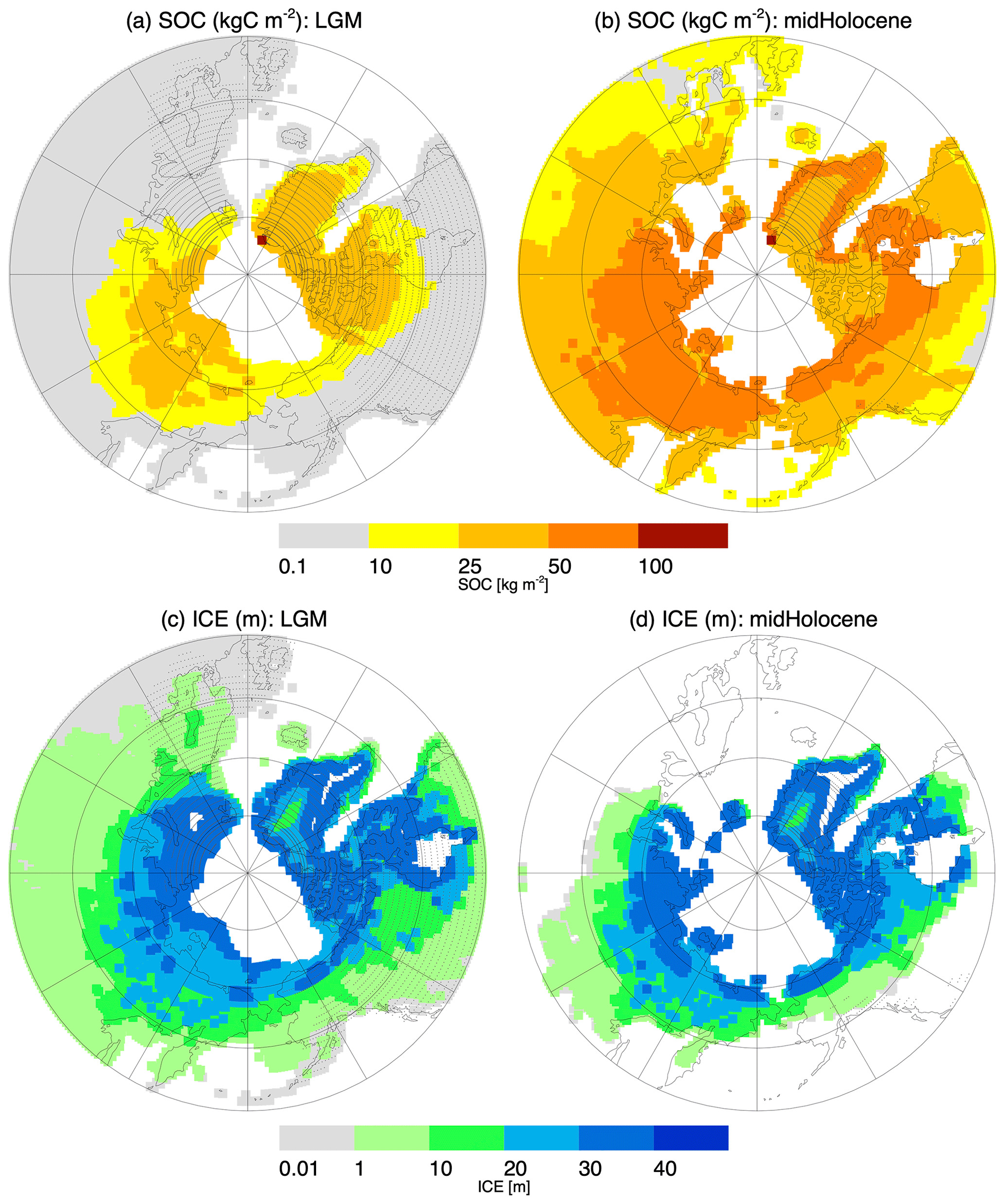
Figure 10 Snapshot maps of SOC and ICE for the periods of the Last Glacial Maximum (LGM, 22 ka) and mid-Holocene (6 ka). The grey dots show areas of ice sheets and glacial cover.

3.3 Implications

3.3.1 Snapshot maps

The simulated time series of SOC, ICE, and soil moisture for each location can be compiled to produce snapshot maps for the area north of 50^∘ N for any period in the last 125 kyr, on the annual basis, if the storage capacity allows. Figure 10 exemplifies the SOC and ICE distributions for the LGM (22 ka, the coldest record in the SeaRISE temperature data in the 23–20 ka window) and mid-Holocene (6 ka, the warmest record for the 8–5 ka window) period for τ=100. A clear and seemingly reasonable contrast between the cold (LGM) and warm (mid-Holocene) climate was observed, although SOC and ICE responded slightly differently. SOC is lower in amount and more contained in extent when the climate was cold, and greater in amount and wider in extent when warm. ICE is widespread but not necessarily greater in amount during the cold environment. In some regions, such as West Siberia, the North Slope in Alaska, and Canadian High Arctic, ICE appeared to continue accumulating until the initiation of the Holocene (see Fig. 6), resulting in the retention of a greater amount of ice under the ground at the mid-Holocene. Note that the SOC and ICE are preserved under the ice sheets (shown by grey dots) until the overlying ice sheet melt (see Sect. 2.3.2).

Another example is the present-day distributions of simulated SOC presented in the accompanying paper (Saito et al., 2020), where we created maps of SOC amounts for each τ at the original 1^∘ resolution and discussed differences in and spatial characteristics of simulated distributions for different values of τ. In addition, we developed a method of associating the value of τ with local topographic–hydrological features derived from a 2 arcmin digital relief model and produced respective high-resolution circum-Arctic maps of SOC and ICE for comparison with currently available observation-based data (i.e. Brown et al., 1998; Hugelius et al., 2014; Olefeldt et al., 2016). These snapshot maps can be used to examine the areal development of variables in the region in the different eras and to produce initial and/or boundary conditions for ESMs or large-scale terrestrial eco-climate models in assessing past or present states, or projecting future impacts on the potential release of GHGs induced by permafrost degradation. Yokohata et al. (2020) partly used the results derived from the present-day snapshot to quantify the relative impacts resulting from the three pathways described in Sect. 1. Such results can provide localized information on the mechanism of permafrost-related GHG releases (e.g. vulnerable areas, potential speed of development) to help stakeholders (i.e. policy and decision makers, as well as residents at local to global levels) adapt to, stabilize, or mitigate climate change consequences.

3.3.2 Future improvements

This study shows the simple framework of the modelling concept and the reconstruction method of forcing/boundary data creation were useful in the reproduction of the evolution and extensive projection of allogenic control, represented by the parameter τ, over long-term carbon dynamics. Nevertheless, there is room for improvement.

The first point relates to the forcing data. This study employed only one ice core dataset to reconstruct the temperature and precipitation history after the last interglacial and used present-day climatology to expand spatially to the circum-Arctic region. Despite a coarse and crude method, (1) it enabled to minimize the degree of subjectivity and uncertainty injected when compiled from different, sometimes contradicting and/or fragmentary, ice core data; and (2) it compensated for the lack of time series of spatially distributed climate data, e.g. outputs from Earth system models, for the entire integration period. This single-core-based dataset successfully produced the first-order approximation of the SOC and ICE evolution in the region that was north of 50^∘ N and demonstrated the model's ability as discussed in Sect. 3.1 and 3.2. Although the driving time series are basically in phase within the simulated circum-Arctic domain, we incorporated some aspects of spatial heterogeneity, e.g. variations of topo-geographical changes in coastlines, altitudes, and ice sheets, as well as the meridional gradient on the amplitude of long-term temperature variations (i.e. polar amplifications). In reality, however, temporal changes in the general circulations and climate patterns have more distinct regional components (Frenzel et al., 1992; Alley et al., 2002; Nakagawa et al., 2003) and behaviours at different timescales (Esper et al., 2002; Cook et al., 2004; Mann et al., 2008). As a result, the initiation timings of the Holocene carbon accumulation were globally heterogeneous as demonstrated by Morris et al. (2018), which the current integration scheme failed to account for (Sect. 3.2.1). In the next step, forcing data should be designed to accommodate information that is more specific to the local history so that the resulting time series and maps can reflect regional diversity and characteristics more adequately.

The second problem relates to the formulation of carbon dynamics (Eqs. 1–3), hydrology (Eq. 4), and ice dynamics (Eqs. 9 and 10). With regard to the quantity in the carbon budget, the calculated litter fall tended to be overestimated, as shown in Fig. 6. Equation (1) was designed to express the upper envelope of the litter fall for the range of temperatures and precipitation levels considered (i.e. −25 to 35 ^∘C and 0 to 600 mm a⁻¹; Fig. 2). Re-evaluation of thermal parameters listed in Table 1 is necessary to account for spatial variations in terms of soil types, microtopography, and geology (sedimentation characteristics). Further, the introduction of a stochastic process to assign a value (e.g. between zero and the currently calculated upper value) according to a statistical distribution (e.g. uniform or Gaussian) is another possibility. Regarding the quality of the carbon process, the evaluation of the decomposition rate κ, and relatedly τ, may be elaborated (Eqs. 1 and 3). As one of the primary objectives of this study was to investigate quantitative impacts and functionality of allogenic (external; climatic or environmental conditioning by T_a, Pr and τ) factors on long-term carbon dynamics, the current model does not specifically consider autogenic (internal, ecosystem-dependent) aspects of the process. However, the examination of the relative contribution of allogenic and autogenic controls on carbon dynamics is important (Lund et al., 2010; van Bellen et al., 2011; Loisel and Yu, 2013; Klein et al., 2013; Charman et al., 2015). Possible structure and processes to be incorporated include multiple pools of different soil carbon stability (labile to recalcitrant) for inputs (i.e. litter fall) and outputs (i.e. rate of decomposition) and their sensitivity to climate and/or hydrology (Boudreau and Ruddick, 1991; Hilbert et al., 2000; Biasi et al., 2005).

As for the hydrological modelling, more rigorous examination for the hydrological parameters, γ and ξ (Eq. 4, Table 1), should be performed using updated datasets, e.g. NASA GLDAS-2 (Li et al., 2019, 2020) and high-resolution soil database (e.g. SoilGrids250m; Hengl et al., 2017). Incorporation of lateral flow of water and resolved carbon may be necessary when the model is to be applied to networked grid points in a specific area (e.g. the North Slope in Alaska or the right bank of the Lena River). Improvement of ice dynamics includes (a) reconsideration of ground ice behaviour when it is covered by large ice sheets (see Sect. 3.1.2), (b) consideration of spatial variability in sediment characteristics (e.g. Canadian shield regions; see also Saito et al., 2020) and vertical profile and physical structure of the subsurface layers for the accumulation of massive ice, and (c) spatial and climatic examination of the heat exchange efficiency parameter β (Eq. 10).

The third problem relates to initial values for carbon and water to be specified for the last interglacial condition. As we had no prior information on initial values for that period, we started the integration with a uniform distribution of both soil carbon and moisture at all grid points north of 50^∘ N. This examination, however, was spatially limited to eight locations. The sensitivity to initial values with larger sets of locations, possibly with a non-uniform distribution (i.e. starting with the present-day distribution under the last interglacial conditions), is worth studying.

4 Conclusions

The spatial distribution of SOC and ICE provides essential information in the assessment and projection of the risks and impacts of permafrost degradation. However, uncertainties related to geographical distribution and the estimated range of the total amount of stored carbon and ice obtained from synchronic compilations of samples or cores continue to be substantial. We adopted a novel approach to estimate present-day spatial distribution and amounts through diachronic simulations. A numerical model (SOC-ICE-v1.0), representing the essential part of the cold-region subsurface carbon and water dynamics by considering frozen ground (permafrost) and land cover changes (ice sheets and coastlines), was developed to calculate the long-term balance of SOC and ICE. The model was integrated for a 125 kyr period from the last interglacial to the present day for areas north of 50^∘ N to simulate accumulations (or dissipations) of SOC and ICE in the circum-Arctic region. Model performance was evaluated using observation-based data and evidence. Although the model was forced by climate data constructed from a single Greenland ice core, the simulated time series reproduced temporal changes in northern SOC and ICE at different climate locations well and successfully captured circum-Arctic regional differences in characteristics. The model provided useful information for quantitative evaluation of the relative importance of allogenic factors to control soil carbon dynamics under different climatological or topo-geographical conditions. The set of simulated results can be compiled to produce snapshot maps of the geographical distributions of SOC and ICE in regions north of 50^∘ N.

Despite its simplicity, the modelling framework employed in this study proved capable of accurately simulating the evolution of the cold-region soil carbon and ground ice, and was powerful enough to provide the spatial distributions in the circum-Arctic. However, some improvements are required in the model, such as the construction of more locally specific forcing climate data series, improvement in the structure and parameterization of soil carbon and ice dynamics, and determination of the initial value distributions for carbon and water integration.