the Creative Commons Attribution 4.0 License.
the Creative Commons Attribution 4.0 License.
 | 12 Aug 2021
Latent Linear Adjustment Autoencoder v1.0: a novel method for estimating and emulating dynamic precipitation at high resolution
Christina Heinze-Deml
Sebastian Sippel
Angeline G. Pendergrass
Flavio Lehner
Nicolai Meinshausen
A key challenge in climate science is to quantify the forced response in impact-relevant variables such as precipitation against the background of internal variability, both in models and observations. Dynamical adjustment techniques aim to remove unforced variability from a target variable by identifying patterns associated with circulation, thus effectively acting as a filter for dynamically induced variability. The forced contributions are interpreted as the variation that is unexplained by circulation. However, dynamical adjustment of precipitation at local scales remains challenging because of large natural variability and the complex, nonlinear relationship between precipitation and circulation particularly in heterogeneous terrain. Building on variational autoencoders, we introduce a novel statistical model – the Latent Linear Adjustment Autoencoder (LLAAE) – that enables estimation of the contribution of a coarse-scale atmospheric circulation proxy to daily precipitation at high resolution and in a spatially coherent manner. To predict circulation-induced precipitation, the Latent Linear Adjustment Autoencoder combines a linear component, which models the relationship between circulation and the latent space of an autoencoder, with the autoencoder's nonlinear decoder. The combination is achieved by imposing an additional penalty in the cost function that encourages linearity between the circulation field and the autoencoder's latent space, hence leveraging robustness advantages of linear models as well as the flexibility of deep neural networks. We show that our model predicts realistic daily winter precipitation fields at high resolution based on a 50-member ensemble of the Canadian Regional Climate Model at 12 km resolution over Europe, capturing, for instance, key orographic features and geographical gradients. Using the Latent Linear Adjustment Autoencoder to remove the dynamic component of precipitation variability, forced thermodynamic components are expected to remain in the residual, which enables the uncovering of forced precipitation patterns of change from just a few ensemble members. We extend this to quantify the forced pattern of change conditional on specific circulation regimes. Future applications could include, for instance, weather generators emulating climate model simulations of regional precipitation, detection and attribution at subcontinental scales, or statistical downscaling and transfer learning between models and observations to exploit the typically much larger sample size in models compared to observations.
- Article
(22083 KB) - Full-text XML
- BibTeX
- EndNote


Precipitation is a key climate variable that is highly relevant for impacts such as floods or meteorological drought. Precipitation simulations at high resolution (e.g. Prein et al., 2017) are required for adaptation planning for local and regional precipitation change in a warming climate. However, precipitation shows large natural variability (Deser et al., 2012), and its relationship with atmospheric circulation is complex and nonlinear, in particular at local to regional scales and in heterogeneous terrain (e.g. Zorita et al., 1995). Moreover, projected changes in precipitation are unevenly distributed across the distribution of precipitation intensity (Allen and Ingram, 2002; Held and Soden, 2006; Pendergrass, 2018). Scaling rates depend on the return period, region, temperature and moisture availability (Prein et al., 2017), and changes in circulation during precipitation events (Shepherd, 2014; Fereday et al., 2018). Hence, it is a key challenge to identify, understand, and interpret patterns of forced precipitation change in model simulations and observations.
Dynamical adjustment techniques have been developed to separate forced and internal variability via a co-interpretation of target variables such as temperature or precipitation using circulation information: a circulation proxy (such as a sea-level pressure pattern) is used to estimate the circulation-induced (dynamic) contribution to temperature or precipitation variability. For example, dynamical adjustment of precipitation has revealed that the spatial pattern and amplitude of observed residual (predominant thermodynamic) precipitation trends at the scale of the entire Northern Hemisphere mid- and high-latitude land areas are in good agreement with the expected anthropogenically forced trends from model simulations (Guo et al., 2019). Similarly, in Europe, Fereday et al. (2018) showed that thermodynamic forced changes in future winter precipitation are in relatively good agreement among models, while large uncertainties remain in simulated forced circulation changes that may affect precipitation. While internal and forced components of precipitation variability and change can be decomposed in large ensembles of model simulations (Deser et al., 2012; von Trentini et al., 2019; Leduc et al., 2019), high-resolution large ensembles are prohibitively expensive. It would be beneficial to be able to estimate and identify forced precipitation patterns from only a few ensemble members at impact-relevant regional spatial scales.
Techniques for dynamical adjustment have relied largely on linear regression (Wallace et al., 1995, 2012; Smoliak et al., 2015; Sippel et al., 2019) or circulation analogue techniques (Yiou et al., 2007; Deser et al., 2016). Because the fraction of variability that can be explained by these techniques is limited, dynamical adjustment has so far been applied on large spatial and temporal scales (e.g. Guo et al., 2019), and has also been more successful for temperature trends than for precipitation. Applying it to precipitation on local or regional scales at high resolution remains a challenge.
In this work, we leverage recent advances in machine learning to propose a novel statistical model – the Latent Linear Adjustment Autoencoder (LLAAE) – suitable for dynamical adjustment (and potentially further applications) in daily, high-resolution precipitation fields. In recent years, deep learning techniques have gained in popularity in machine learning due to large improvements in neural network architectures, optimization algorithms as well as computing power and frameworks. Among the class of deep generative models, the introduction of variational autoencoders (VAEs) (Kingma and Welling, 2014; Rezende et al., 2014) started a whole subfield in deep learning research. Among other things, the popularity of VAEs is due to their ability to generate new images, in addition to being a powerful nonlinear dimensionality reduction technique. Our proposed Latent Linear Adjustment Autoencoder extends the standard VAE model appropriately to enable the climate applications of interest.
Specifically, during training, the Latent Linear Adjustment Autoencoder encodes daily precipitation fields into a low-dimensional latent space and subsequently decodes them for reconstruction. In addition, we formulate the objective function such that the latent space can be regressed linearly on the circulation proxy. For dynamical adjustment, we use the estimate of the latent space based on circulation, which is then decoded for predicting daily precipitation fields at high spatial resolution. In other words, the final model is nonlinear, consisting of a linear part and a nonlinear part, where the latter is a deep neural network. It enables prediction of the portion of the precipitation field that can be explained by circulation (i.e. the dynamic component of precipitation). Moreover, several further climate science applications of the Latent Linear Adjustment Autoencoder are conceivable, such as for example weather generators emulating regional climate model simulations, detection and attribution at subcontinental scales, or statistical downscaling, and are discussed further below.
In summary, the objectives of this paper are the following:
-
We introduce a novel statistical model – the Latent Linear Adjustment Autoencoder – as a versatile technique for applications in climate science, particularly for making better use of high-resolution climate simulations by estimating circulation-induced (dynamic) precipitation at high resolution from coarse-scale circulation information.
-
We illustrate the Latent Linear Adjustment Autoencoder by applying it to dynamical adjustment of daily high-resolution precipitation from simulations over central Europe. More specifically, the LLAAE will be used to separate forced precipitation trends from internal variability.
Following Smoliak et al. (2015) and Sippel et al. (2019), we frame dynamical adjustment as a statistical learning problem. Let be the climate variable of interest on a spatial field of size h×w and let X∈ℝp be input features. In the following, we consider daily precipitation fields for Y and empirical orthogonal function (EOF) time series of sea-level pressure (SLP) for X as a proxy for circulation. The EOF time series are detrended (as described below) and scaled to unit variance; in the EOF computation, we do not weight by area. A variety of climate variables instead of precipitation could be taken as Y; results for daily temperature can be found in Appendix C.
Let X be the n×p matrix, where each column contains one input feature with n data points. Each data point is in our case a simulation from a regional climate model (RCM), and each column corresponds to one of p EOF components of SLP, from the RCM but at coarsened resolution. Let Y be the tensor that represents the precipitation intensity for each data point in a spatial field. Below, we present our proposed statistical model, which estimates the circulation-induced component of precipitation :
where f is a generic nonlinear function. Let denote the residuals that remain. Since is the precipitation explained primarily by variations in circulation, is the precipitation primarily unexplained by circulation. If SLP is unaffected by external forcing, then this residual contains the signal induced by the thermodynamic component of the external forcing, since the variability due to circulation has been removed. If instead external forcing does affect SLP, then the dependence between X and Y that arises due to the common influence of the external forcing would bias the estimation of f. To avoid potential forced trends in SLP projecting onto the thermodynamic component of the external forcing in Y, we detrend the daily SLP EOF time series as follows. We ensure that they are orthogonal to the smoothed, first EOF of the January ensemble mean by regressing the time series against the ensemble mean and using the corresponding residuals as input features X. The reasoning behind this step is that a forced trend in SLP will be approximately captured in the first EOF of the SLP ensemble mean. Here, we use the January ensemble mean as a proxy for December–February SLP. For simplicity, we refer to the detrended and scaled SLP EOF time series simply as the “SLP time series” in the following.
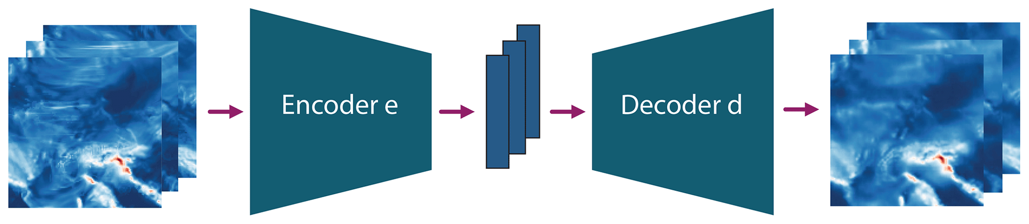
Figure 1Illustration of a standard autoencoder model: the spatial fields Y are fed to the encoder e which maps them to the latent space variables L (illustrated in blue). These are in turn fed to the decoder d which computes a reconstruction of the input, .
2.1 Latent Linear Adjustment Autoencoder: proposed deep autoencoder model for dynamical adjustment
We build on variational autoencoders (Kingma and Welling, 2014; Rezende et al., 2014), which can be understood as a (typically nonlinear) dimensionality reduction method. An autoencoder consists of an “encoder” e that maps Y to the low-dimensional latent space L∈ℝl, L=e(Y), and a “decoder” d which in turn maps L to the reconstruction of Y, . This scheme is illustrated in Fig. 1, which depicts the reconstruction of precipitation fields. The VAE objective encourages the distribution of the latent space variables L to be close to a chosen prior distribution, typically a standard multivariate Gaussian distribution, and also ensures that . The encoder and the decoder are parameterized as (deep) neural networks.
We extend the standard VAE model to make it suitable for dynamical adjustment by adding a linear component h to the architecture. The linear component h takes X as input features and predicts the latent space variables L of the VAE; thus, we call the overall model the “Latent Linear Adjustment Autoencoder”. Using an appropriate training objective (see Eq. 3), we enforce that when linearly predicting the latent space variables L with X, , the resulting decoded prediction to be close to Y. The motivation behind this loss function is that the combined model, which consists of the combination of h and d, should explain as much variance in Y as possible, while using only the input X. In other words, it should capture the circulation-induced signal in Y. The advantage of combining the linear model h with the nonlinear decoder of the VAE d is that the overall model is very expressive, while the estimation of h remains relatively simple.
In more detail, we consider the following objective to train the encoder e and decoder d with associated parameters of our proposed Latent Linear Adjustment Autoencoder:
ℒVAE is the standard VAE objective for real-valued input data, consisting of a reconstruction loss and the Kullback–Leibler divergence between the distribution of the encoded inputs and the prior distribution of the latent space, here chosen to be a standard multivariate Gaussian distribution (for details, see Kingma and Welling, 2014; Rezende et al., 2014). ℒL is the extension to the objective that we propose:
and λ is a tuning parameter that steers the relative importance of the two loss functions in the overall objective (Eq. 2). The autoencoder and the linear model are trained iteratively in an alternating fashion. In the first step, the objective ℒθ is optimized while h is treated as fixed. In a second step, the linear component h of the Latent Linear Adjustment Autoencoder is trained with squared error loss, treating the encoder and decoder parameters as fixed:
The parameters of the encoder and decoder (θe,θd) and those of the linear model h, θh, are coupled, since the linear model aims to predict the latent space variables L, which are subject to change during the training of the encoder and the decoder. At the same time, the autoencoder should be trained such that a linear regression from L on X achieves a small error in Eq. (3), which is accomplished with this procedure for training the components. In practice, we train the model using the Adam optimizer (Kingma and Ba, 2015). All details related to training the model, such as architecture and hyperparameter choices, as well as code to reproduce our experimental results, can be found in Appendix A.
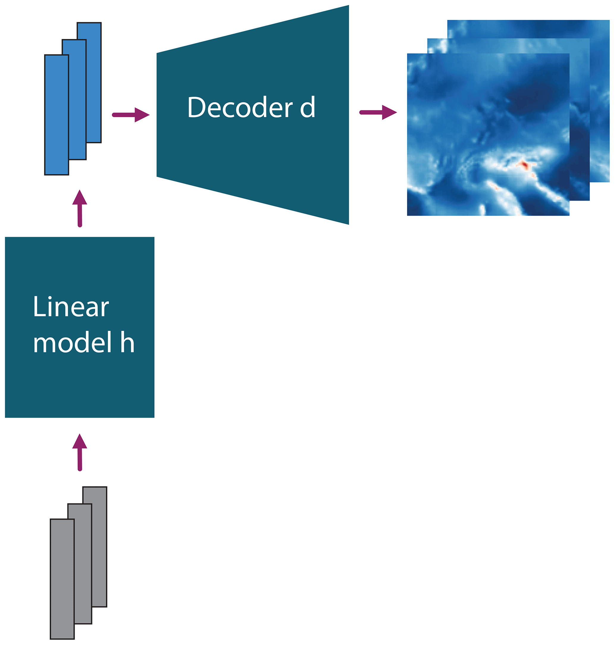
Figure 2Illustration of the Latent Linear Adjustment Autoencoder after training: the input features X (illustrated in grey) are fed to the linear model h which yields a prediction for the latent space variables L (illustrated in light blue). These are in turn fed to the decoder which computes a prediction of the spatial field based on X only, . Training the models e, d, and h is performed iteratively in an alternating fashion.
After training the components e, d, and h, we no longer need the encoder to perform dynamical adjustment on unseen test data. This is illustrated in Fig. 2. We predict the latent space variables with the linear model h using the SLP time series as input X. The resulting predictions are fed to the decoder, which outputs predictions of the spatial field based only on X. In other words, we obtain the spatial field of precipitation which can be explained by circulation.
The spatial field is modelled jointly in our approach – the optimization is performed over the whole spatial field at once – in contrast to Sippel et al. (2019), where a separate model needed to be trained for each grid cell. The joint modelling of the daily high-resolution precipitation field as a function of coarse-scale circulation may enable several additional climate science applications, which are briefly discussed in Sect. 4.
3.1 Data
To evaluate our statistical model, we use the Canadian Regional Climate Model Large Ensemble (CRCM5-LE, Leduc et al., 2019) which is based on a dynamically downscaled version of the 50-member CanESM2 large ensemble (CanESM2-LE). CanESM2-LE is an initial-condition ensemble of climate change projections (Kirchmeier-Young et al., 2017) run with the Canadian Earth System Model (Arora et al., 2011), globally on a spatial resolution of 2.8∘. CanESM2-LE combines so-called “macro” and “micro” initializations: to achieve different 1950 ocean states (the macro initialization), five historical spinup runs are branched from a long pre-industrial (1850) control run to which small random atmospheric perturbations and then time-varying forcings are applied until 1950. Then, for the micro ensemble (where members have the same initial conditions in the ocean but differ in their atmosphere), a second set of random perturbations is applied in 1950 to generate 10 runs spanning 1950–2006 for each of the five historical spinups, with a time-varying historical forcing scenario applied through 2006. The runs continue from 2006 until 2100 with RCP8.5 forcing (Kirchmeier-Young et al., 2017).
This approach yields 50 approximately independent realizations of the climate system (Leduc et al., 2019). Each of the global simulations has been downscaled using the Canadian Regional Climate model version 5 (Martynov et al., 2013) to a resolution of approximately 0.11∘ (≈ 12 km) over Europe for the 1950–2099 period, which yields the regional large ensemble CRCM5-LE. More details about the modelling setup and evaluation of the simulations are available in Leduc et al. (2019).
3.2 Experimental setup
3.2.1 Target variables
We focus on precipitation as the target climate variable throughout the main text. A subset of results for temperature can be found in Appendix C. For the precipitation fields, we apply a square-root transformation to stabilize the autoencoder training; the results presented in Sect. 4 are based on transforming the results back to the original scale (mm d−1), except for some visualizations where indicated in the captions. The spatial fields we consider have 128 × 128 grid cells; i.e. they are a subset of the original 280 × 280 field, cropped around central Europe (with boundaries 42–54.8∘ N, 0–18.9∘ E). We aggregate the data (which are hourly) to daily averages.
3.2.2 Input features
SLP is regridded to a spatial resolution of 1 × 1∘ before computing the EOFs as described in Sect. 2, so that the model predicts high-resolution precipitation from only a coarse-resolution proxy of atmospheric circulation. We aggregate the data (3 h) to daily averages. SLP data are also taken from the original 280 × 280, 0.12∘ resolution Coordinated Regional Climate Downscaling Experiment – European Domain (EURO-CORDEX) (WCRP, 2015) and regridded to a regular 1 × 1∘ grid that broadly covers the region of −15 to 35–64∘ N, 35∘ E (see Fig. 9, top).
3.2.3 Time periods and training/test splits
We use RCM simulation data from 1955 to 2100 to allow for 5 years of spinup. We train our model using daily data from December to February (DJF) from nine ensemble members (“kba”, “kbc”, “kbe”, “kbg”, “kbi”, “kbk”, “kbm”, “kbq”, “kbs”). The results in the main text are based on training data that comprise the years 1955–2070. In Appendix B, we present results based on the shorter training time period from 1955 to 2020, using the same ensemble members. This corresponds to a reduction in the amount of training data points of approximately 43 % and serves as a sensitivity test to the amount of training data. Furthermore, we evaluate our trained models on the remaining 41 ensemble members that were left out of training. We refer to these as “holdout ensemble members”.
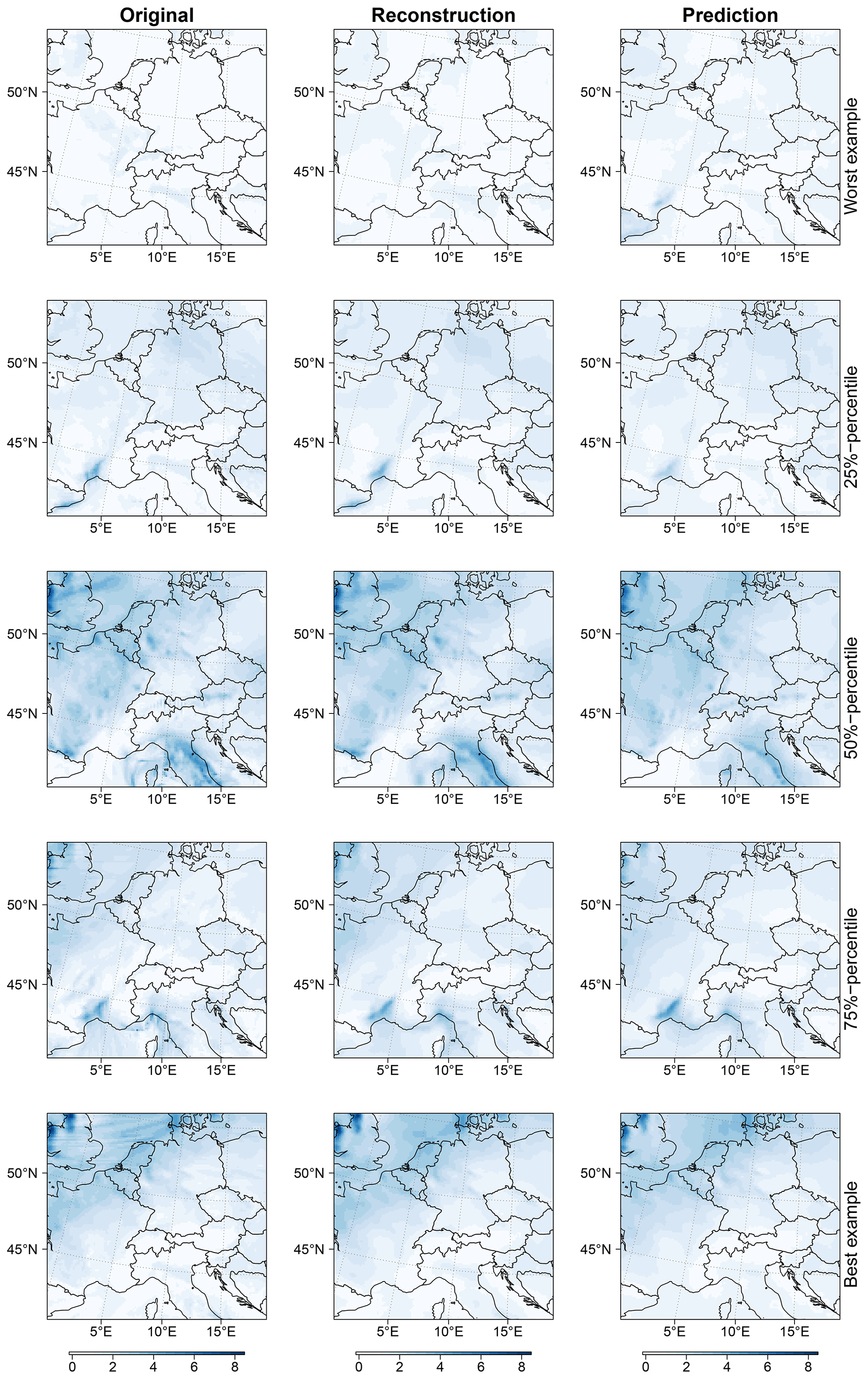
Figure 3Examples of (i) original precipitation fields (left column), (ii) reconstructions (centre column), and (iii) predictions (right column). The examples are chosen such that the R2 value of the prediction increases from top to bottom: the first row shows the worst example in the holdout dataset, the last row shows the best example, and the remaining rows show examples at the 25th, 50th, and 75th percentiles, respectively. For better visibility, data are square-root transformed. Hence, the units are .
3.2.4 Evaluation of predictions
To illustrate the spatial coherence of our approach, we show five example target (daily) data points of Y, their reconstructions , and the predictions from the holdout ensemble member “kbb” (Fig. 3). These examples are chosen for different percentiles of the distribution of the R2 values (i.e. proportion of explained variance). As such, they show the range between data points where the LLAAE performs relatively poorly to cases where the LLAAE performs well (in terms of R2). To highlight the precipitation features, these examples are displayed after the data have been square-root transformed. We compute the grid-cell-wise mean squared error (MSE) of predictions and the proportion of explained variance (R2) based on the daily data from the holdout ensemble member “kbb”. The results for the other holdout ensemble members are very similar. We further evaluate the predictions within a dynamical adjustment framework described in the next paragraph.
3.2.5 Dynamical adjustment
We evaluate the extent to which the forced response of precipitation can be uncovered with a small number of ensemble members using dynamical adjustment (e.g. Deser et al., 2016). Specifically, we quantify how well the long-term “forced response” (i.e. the average across all 50 ensemble members) can be approximated by the residuals of our predictions (the difference between precipitation simulated by the RCM and the circulation-induced component of precipitation predicted by the Latent Linear Adjustment Autoencoder). In other words, dynamical adjustment acts as a filter for short-term “circulation-induced” precipitation variability. Recall that we expect the residuals to primarily contain the thermodynamic component of change (Deser et al., 2016). However, it is important to stress that the residual is not a perfect proxy for thermodynamical change, because it may contain effects from feedbacks, remaining internal variability, and circulation components not directly captured by SLP. Moreover, since the SLP data are detrended prior to the application of the method, long-term dynamical changes may even be part of the residuals. In addition to analysing the forced response in seasonal precipitation totals, we evaluate the estimation of the forced precipitation response for two composites of atmospheric circulation based on EOF analysis of SLP.
4.1 Reconstructed and predicted spatial fields
We begin by showing a selection of reconstructed precipitation fields from the holdout ensemble member “kbb” (centre, Fig. 3), which illustrates the skill of the encoder and decoder, and predictions (right, Fig. 3), which illustrate the skill of the linear latent model h against the original RCM-simulated precipitation Y (left, Fig. 3). The reconstruction quality, i.e. the similarity between the left and the centre column, is quite high, though not all fine details are reproduced (which is to be expected). The predictions (right column) are computed using the linear model h and the decoder d with SLP time series as inputs. For the worst example (in terms of R2; first row), the original spatial field shows that this corresponds to a day with very low precipitation, while the LLAAE predicts larger precipitation in some regions (e.g. south of France), resulting in a very low R2 value. For the other rows (25 % percentile – best example), the predictions resemble the original image fairly well. For dynamical adjustment, we use the residuals , which are computed as the difference between the original fields Y (left column) and the predictions (right column).
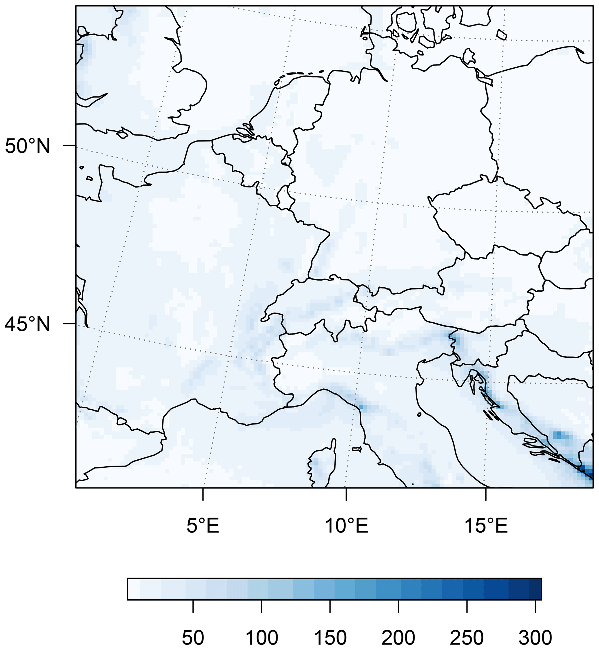
Figure 4MSE (based on precipitation data in mm d−1) for each grid cell for the precipitation predictions.
The proposed model yields spatially coherent predictions and explains a large proportion of the variance of Y. The skill of precipitation predicted with the Latent Linear Adjustment Autoencoder is quantified in Fig. 4, which shows the grid-cell-wise MSE over all December–February days for the holdout ensemble member “kbb”. The spatial pattern of MSEs (Fig. 4) largely reflects the pattern of precipitation as simulated by the RCM. Prediction errors are high over heterogeneous terrain, likely linked to orographic precipitation, in particular on the western sides of mountain ranges such as the Alps in central Europe, the Appenines in Italy, the Dinaric Alps in southeastern Europe, and smaller ranges located in France and Germany. Prediction errors are also high at the west coast of the UK, whereas mean squared prediction errors appear relatively low over low-altitude regions (e.g. northern France, Benelux, and north Germany). The spatial pattern of R2 (the fraction of explained variance, Fig. 5) shows a more nuanced pattern dominated by a land–sea contrast. Over land, the circulation proxy generally explains a high proportion of variance (up to ≈ 90 %), especially on the western slopes of mountain ranges, which receive a large fraction of their precipitation from large-scale circulation-induced events. In contrast, the fraction of variance explained by circulation-induced precipitation is smaller on the eastern sides of mountain ranges, and particularly low over oceanic regions (which we do not interpret in this study).

Figure 5Proportion of variance explained (R2) for each grid cell for the precipitation predictions.
4.2 Extraction of forced precipitation trends at high spatial resolution
In this subsection, we evaluate our predictions of the circulation-induced component in the framework of dynamical adjustment (Deser et al., 2016). That is, we test the extent to which the forced response of regional high-resolution precipitation obtained from averaging across the full 50-member ensemble can be approximated by the residuals of our predictions from a single or from relatively few ensemble members. The thermodynamic component of the variation in precipitation, which is driven by temperature change and unrelated to dynamically induced variability, should remain in the residuals (e.g. Deser et al., 2016). Dynamical adjustment hence acts to reduce short-timescale circulation-induced variability, thus increasing signal-to-noise ratios of the long-term, forced component (Deser et al., 2016).
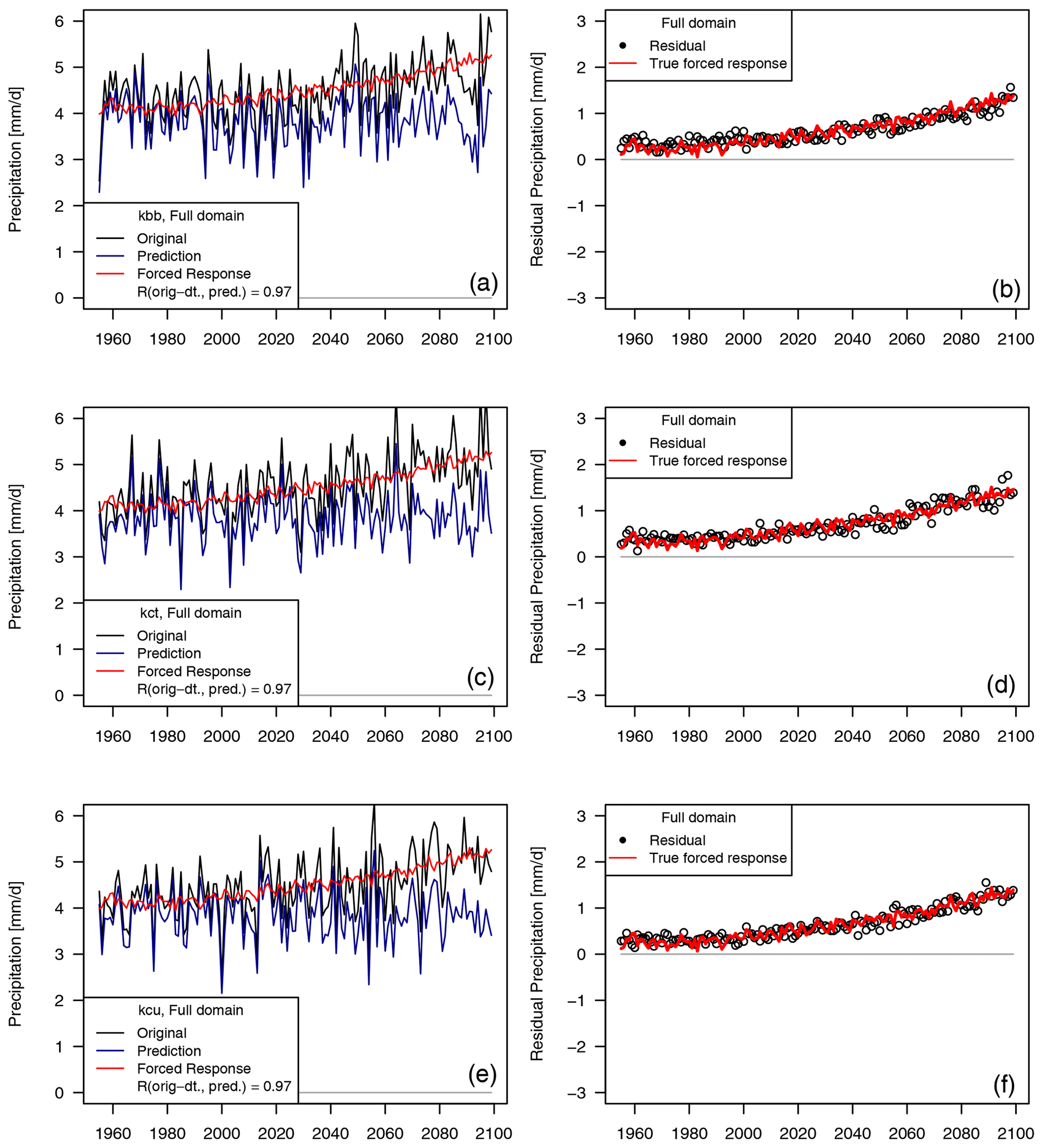
Figure 6Dynamical adjustment of the full domain (land grid cells only) using autoencoders; (left) seasonal precipitation totals simulated by three members of the high-resolution RCM in black (top: “kbb”, middle: “kct”, bottom: “kcu”), the predicted (“circulation-induced”) component for three “holdout” ensemble members (blue), and the forced response (average across all 50 members, red); (right) residuals from the prediction (black dots) and the forced response (red).
The effect of dynamical adjustment can be seen in Fig. 6. It shows time series of domain-average (land only) December–February seasonal precipitation totals simulated by the high-resolution RCM, the predictions of the circulation-induced component for three holdout ensemble members, and the forced response. All three RCM ensemble members show an increasing trend in seasonal precipitation totals across the 21st century, over which large interannual variability is superimposed. In contrast, the predicted circulation-induced components capture the interannual precipitation variability well, but they do not show discernible trends. Consequently, the residuals have relatively smoothly increasing trends, which match the magnitude of the forced precipitation trend well (Fig. 6, right panels). This demonstrates successful dynamical adjustment of continental-scale seasonal precipitation totals using the Latent Linear Adjustment Autoencoder.
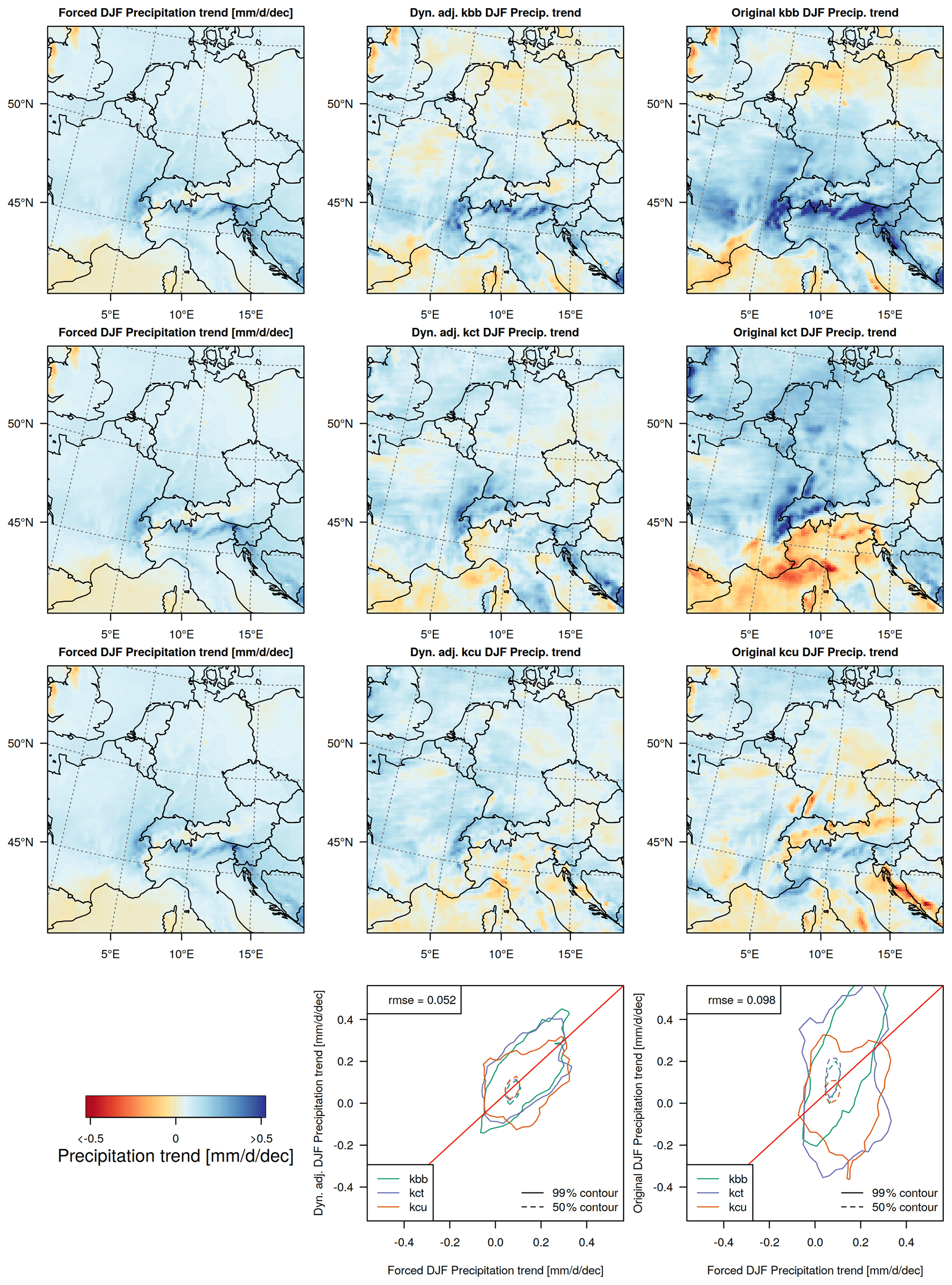
Figure 7Dynamical adjustment of 50-year winter precipitation trends (2020–2069); (left column) forced precipitation response (2020–2069 linear winter precipitation trends averaged over all 50 ensemble members); (middle column) linear 50-year winter precipitation trends in three randomly selected dynamically adjusted ensemble members (top: “kbb”, middle: “kct”, bottom: “kcu”); (right column) linear 50-year winter precipitation trends in the original ensemble members (top: “kbb”, middle: “kct”, bottom: “kcu”); (bottom row) scatter plot contour lines of 50-year precipitation trends in the forced response against 50-year precipitation trends over land in dynamically adjusted (middle) and originally simulated ensemble members (right).
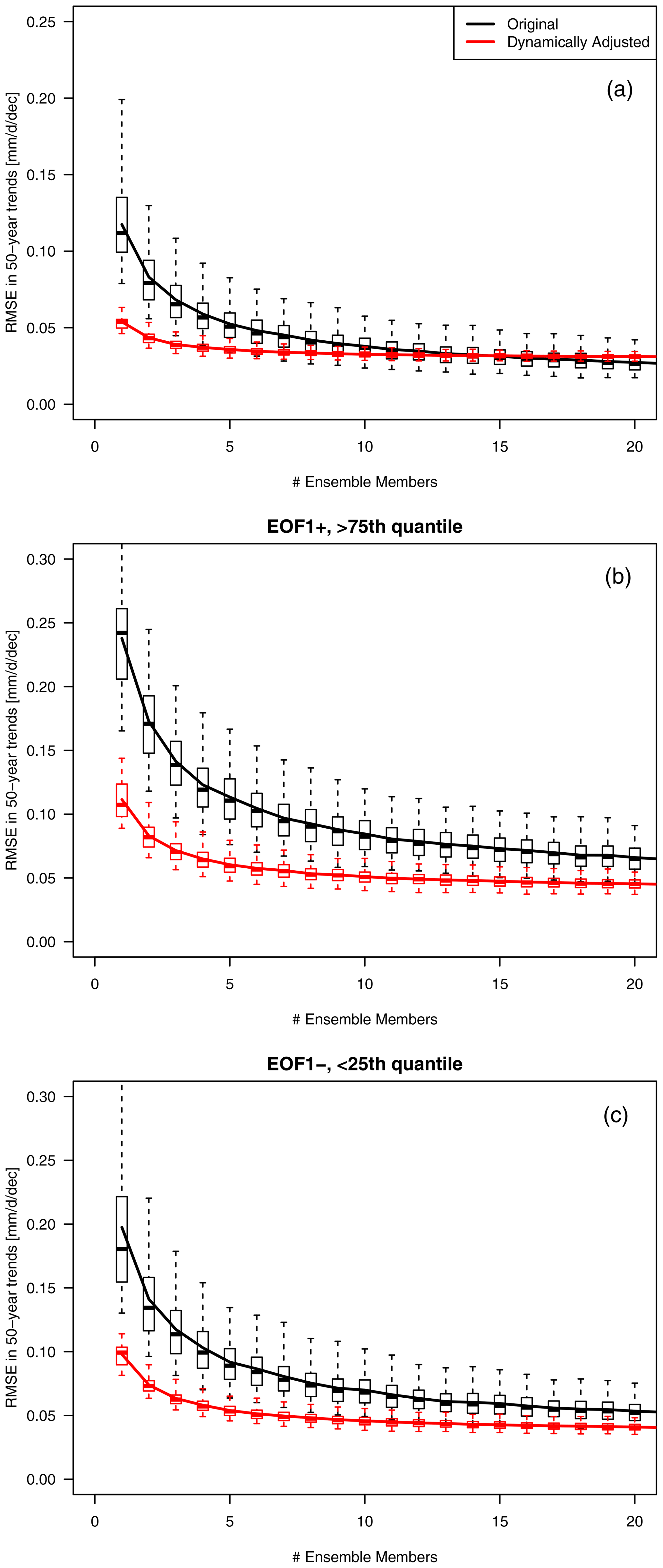
Figure 8RMSE of 50-year trends, calculated by averaging n members, compared to 50-year trends using 50-member ensemble average (“forced response”). RMSEs are based on land grid cells only and shown for averaging n original ensemble members (black) and averaging n dynamically adjusted ensemble members (red). Trends are calculated over the entire DJF season (a) and only for EOF1+ (b) and EOF1- situations (c). Boxplot whiskers indicate 2.5th and 97.5th percentiles (boxes show 25th and 75th percentiles) of RMSE distribution obtained from bootstrapping from the 41 holdout ensemble members.
It is more challenging, however, to identify and evaluate the forced precipitation response at the local scale of individual grid points. To this end, Fig. 7 shows the spatial pattern of forced 50-year (2020–2069) precipitation trends, the pattern of dynamically adjusted precipitation trends, and “raw” precipitation trends in RCM simulations for three holdout ensemble members. The forced response of winter precipitation change is dominated by a north–south contrast. The northern part of the domain is projected to experience a precipitation increase in the 21st century, while decreases in precipitation are projected for the southernmost part of the domain (mainly over the Mediterranean Sea). Increases in winter precipitation across most parts of the domain are largely due to thermodynamic and lapse rate changes (e.g. Brogli et al., 2019). Locally, forced precipitation trends are larger over heterogeneous terrain, which may be due to forced dynamic components that are independent of SLP (Shi and Durran, 2014). The latter paper shows idealized simulations of the forced response of orographic precipitation, which is dynamic, but it is driven by changes in vertical velocity on the upslope side that enhances orographic precipitation, which could be separate from the changes in upslope wind speed and thus SLP. Vertical velocity could increase because of the increasing moisture with warming.
However, large variability in individual ensemble members is superimposed on the signal of forced change (Fig. 7, right), consistent with the large role of internal variability even on multi-decadal timescales (Leduc et al., 2019). For example, ensemble member “kct” (second row) produces a relatively strong drying trend over northern Italy, which is entirely due to internal variability. The dynamically adjusted version of “kct” shows only very weak drying in northeastern Italy, whereas it shows an increased precipitation trend consistent with the forced response at all other locations in northern Italy. Similar differences can be seen between the adjusted and unadjusted trends for the other holdout ensemble members. Overall, the correlation of 50-year trends at a single location from a single ensemble member with the trend in the 50-member forced response is rather low (R=0.4, RMSE = 0.098). However, the dynamically adjusted single ensemble members are more strongly correlated with the forced response and capture it more accurately (R=0.58, RMSE = 0.052).
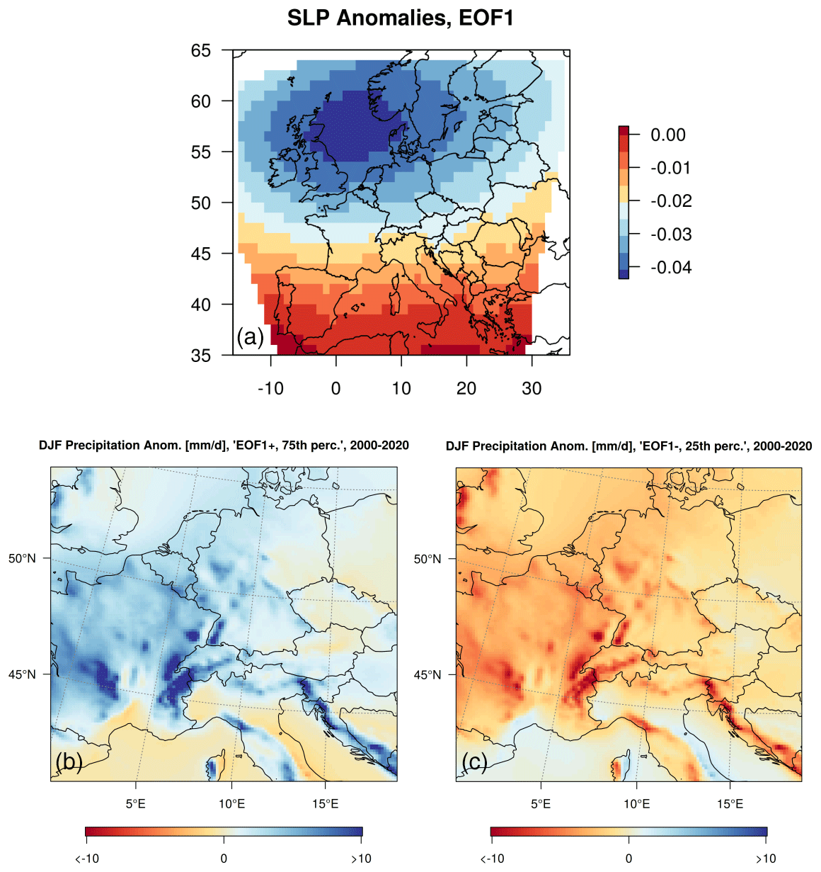
Figure 9(a) First empirical orthogonal function of sea-level pressure over the full domain of the regional model. (b, c) Winter precipitation anomalies for the 25 % of days that show the strongest (b) and weakest (c) projection on the pattern of the first EOF (i.e. days with a strong zonal SLP gradient and hence dominant westerly flow, b, and days with weak to absent zonal SLP gradients, c).
Figure 8 (top panel) shows the RMSE for the reconstruction of forced 50-year precipitation trends (i.e. the 50-member average), via dynamical adjustment and the averaging of original ensemble members, as a function of the number of ensemble members n. With an increasing number of ensemble members (n), the reconstruction RMSE of the forced response is considerably reduced. Hence, dynamical adjustment is particularly useful when only few members are available, e.g. for small ensembles up to five members. If only one member is available, the reconstruction RMSE of the forced 50-year precipitation trend is reduced by more than half via dynamical adjustment. Conversely, to achieve the same RMSE of a single dynamically adjusted ensemble member, an ensemble average of about four to six members would be required (Fig. 8, top panel). On the other hand, for ensembles with more than about 14 members, dynamical adjustment does not improve the ability to reconstruct the forced response. Moreover, dynamical adjustment reduces not only the reconstruction RMSE but also reduces the spread of the distribution across ensemble members, as indicated by the boxes and whiskers in Fig. 8 (top panel). The overall reduction of the reconstruction RMSE also holds particularly for specific circulation regimes (Fig. 8, middle and bottom panels) and is discussed in the next subsection.
4.3 Elucidating forced precipitation trends for specific circulation composites at high spatial resolution
While dynamical adjustment of long-term trends of temperature and precipitation has become a standard tool for the detection of forced thermodynamic trends (Smoliak et al., 2015; Deser et al., 2016; Guo et al., 2019; Lehner et al., 2018), a bigger challenge is to assess forced trends in specific circulation regimes. One example would be summer heat waves related to specific circulation conditions (Jézéquel et al., 2018).
Thus, we assess to what extent the forced precipitation response can be uncovered under specific circulation conditions from a small number of ensemble members. We create composites of the dominant mode of atmospheric winter circulation over Europe as diagnosed by EOF analysis over the historical period (1955–2020) in the RCM simulations. The first EOF of the coarse-resolution SLP field is shown in Fig. 9 (top). The dominant mode has a meridional gradient, with low-pressure anomalies over northern Europe and high-pressure anomalies over the Mediterranean. Although the domain includes only a small fraction of the North Atlantic, the dipole character of the EOF spatial pattern resembles the North Atlantic Oscillation (NAO).
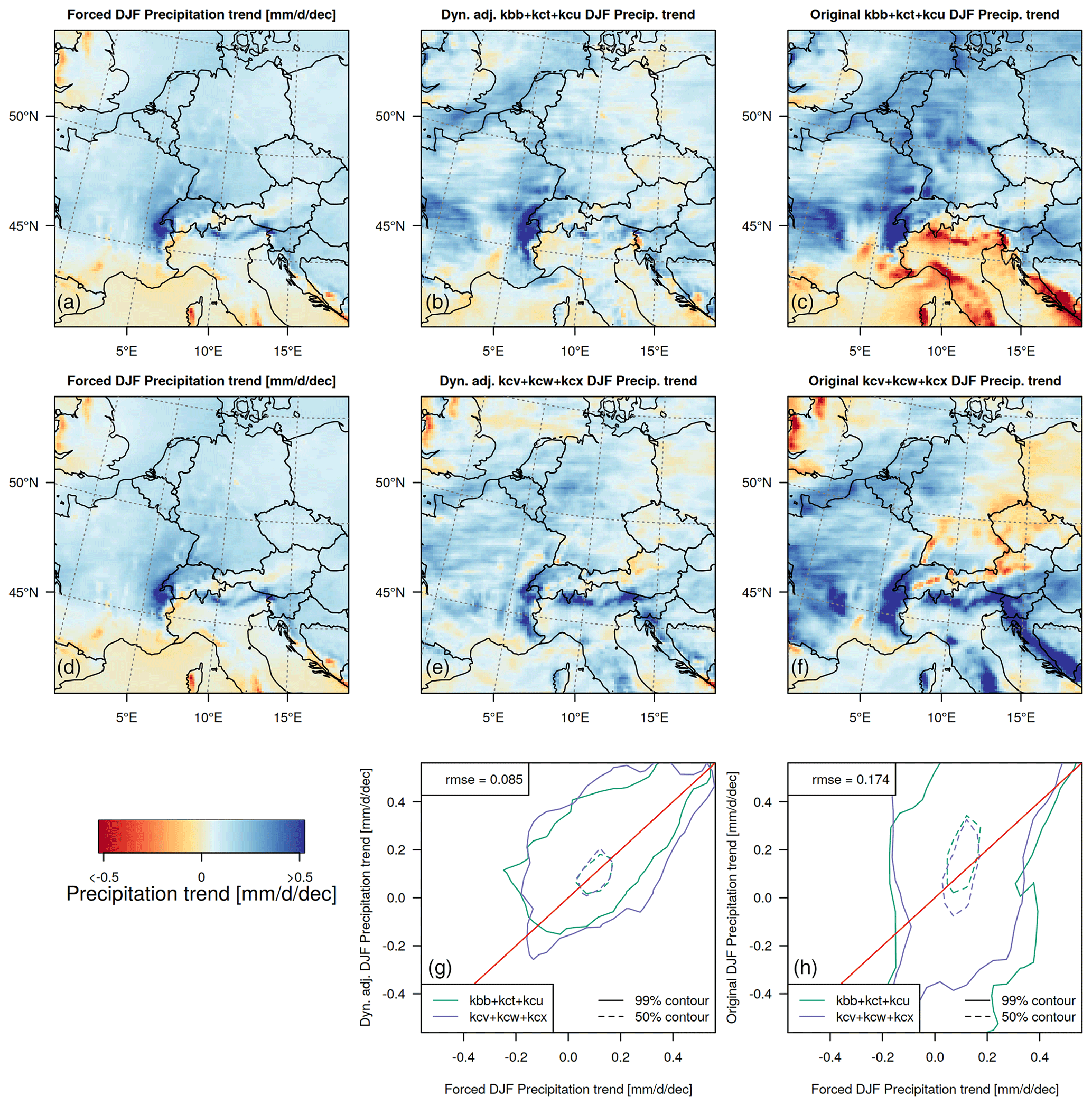
Figure 10Dynamical adjustment of 50-year winter precipitation trends (2020–2069) under the “EOF1+” regime (25 % of all days that project strongest on the first EOF, i.e. those that show a strong westerly flow). (a, d) Linear forced winter precipitation trends under the “EOF1+” regime (2020–2069). (b, e) Linear 50-year winter precipitation trends in an average of three randomly selected dynamically adjusted ensemble members. (c, f) Linear 50-year winter precipitation trends in an average of three corresponding original ensemble members. (g, h) Scatter plots of 50-year precipitation trends in the forced response against 50-year precipitation trends over land in dynamically adjusted (g) and originally simulated ensemble members (h).
We now generate composites of “EOF1+” and “EOF1-” regimes by isolating days that exceed the 75th percentile (“EOF1+”) and those that fall below the 25th percentile (“EOF1-”) in terms of the first principal component (Fig. 9, bottom). Note that the principal component time series associated with EOF1 does not show any discernible trend until the late 21st century, so we do not expect large forced changes in the SLP variability patterns over Europe. On winter days with strong positive EOF1 (“EOF1+”, roughly analogous to NAO+), i.e. a pronounced north–south pressure gradient, increased westerly winds bring mild and moist air from the Atlantic into central Europe (Fig. 9, bottom left). Conversely, the opposite regime suppresses westerlies, hence inducing drier conditions on average (Fig. 9, bottom right) which are also accompanied by colder temperatures.
For the 50-year forced precipitation trend on “EOF1+” winter days (obtained by averaging across all ensemble members), there is a more pronounced precipitation increase on the western slopes of the Alps and in most parts of the domain north and west of the Alps (Fig. 10, left panel). Meanwhile, precipitation decreases in the EOF1+ regime over southern Europe.
Raw simulations for sets of three holdout members show variable 50-year (2020–2069) precipitation trends under the “EOF1+” regime (Fig. 10, right panel), where the spatial pattern of each set of three averaged members only weakly resembles the forced pattern (RMSE = 0.174). The dynamically adjusted holdout members reveal a pattern that more closely resembles the forced response pattern (Fig. 10, middle panel), where forced changes in mountainous regions are particularly well captured; the pattern RMSE is reduced substantially (RMSE = 0.085).
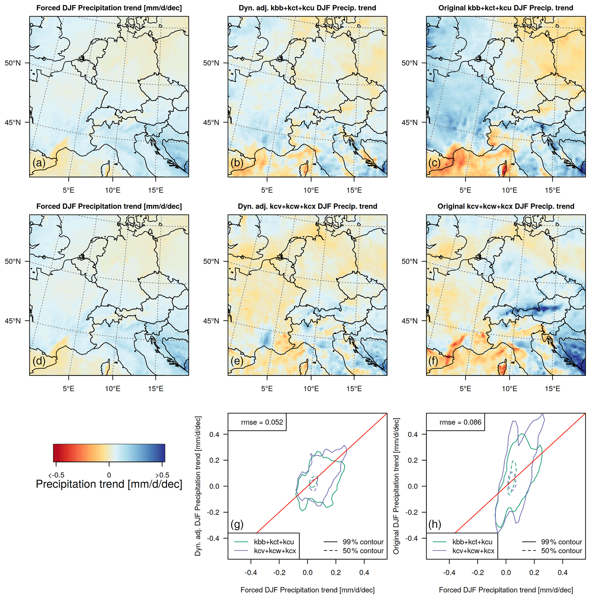
Figure 11Dynamical adjustment of 50-year winter precipitation trends (2020–2069) under the “EOF1-” regime (25 % of all days that project weakest on the first EOF). (a, d) Linear forced winter precipitation trends under the “EOF1-” regime (2020–2069). (b, e) Linear 50-year winter precipitation trends in an average of three randomly selected dynamically adjusted ensemble members. (c, f) Linear 50-year winter precipitation trends in an average of three corresponding original ensemble members. (g, h) Scatter plots of 50-year precipitation trends in the forced response against 50-year precipitation trends over land in dynamically adjusted (g) and originally simulated ensemble members (h).
Forced precipitation trends for 2020–2069 under “EOF1-” conditions differ from “EOF1+” conditions due to a change in the synoptic situation: the forced spatial pattern has generally weaker precipitation changes (due to overall drier conditions during “EOF1-”), and precipitation increases are confined towards southeastern Europe (Fig. 11, left panel). Meanwhile, over large regions north and west of the Alps, precipitation changes only weakly under these circulation conditions. Spatial patterns of dynamically adjusted ensemble members (Fig. 11, middle panel) have a closer correspondence to the forced pattern than to the spatial patterns of “raw” 50-year trends (Fig. 11, right panel). The reconstruction RMSE of the forced response is again substantially reduced (RMSE = 0.052 for dynamically adjusted grid cells; RMSE = 0.086 for raw trends).
The application of dynamical adjustment to composites of specific circulation regimes raises the question as to whether the Latent Linear Adjustment Autoencoder may be applicable to understanding the dynamical component in extreme precipitation events. While the LLAAE may be able to fill an important gap in reconstructing the dynamical component of daily precipitation fields, possibly including days with extreme precipitation (at least, the component proportional to surface pressure), it exhibits a tendency to smooth predicted precipitation fields (Fig. 3), which would presumably result in somewhat underpredicted extreme events. However, a detailed evaluation of the LLAAE in the context of extreme events will be the focus of future work.
Overall, we conclude that dynamical adjustment enables approximating the forced response from high-resolution simulations with only a few ensemble members. This is possible for both long-term trends in seasonal precipitation totals as well as for trends under more specific circulation regimes. The improvement for the “EOF1+” and “EOF1-” circulation regimes can be evaluated from Fig. 8 (middle and bottom panels), where reconstruction RMSEs of forced 50-year precipitation trends, based on one ensemble member, are reduced by up to about a factor of 2 by using dynamical adjustment based on the Latent Linear Adjustment Autoencoder. To achieve a similar forced response reconstruction RMSE, an ensemble average of about four to six members would be required (Fig. 8) both for seasonal trends (top panel) and the trends under specific circulation composites.
4.4 Dynamical adjustment uncertainties, computational costs, and future applications
One of the main uncertainties in dynamical adjustment is the question of whether and how to detrend the climate data (circulation fields and/or precipitation) prior to dynamical adjustment. This is somewhat subjective and often discussed as an inherent uncertainty in the literature (see, e.g. Deser et al., 2016; Lehner et al., 2017, 2018, for a discussion about trend removal). Forced changes in European winter SLP are highly uncertain, and models disagree on the sign and patterns of forced circulation change (Fereday et al., 2018), while thermodynamic aspects are typically considered more robust across models (Shepherd, 2014; Fereday et al., 2018). Therefore, it is critical to ensure that the statistical model does not fit a thermodynamical forced signal and hence only models the dynamical variability. For the results presented in this work, we orthogonalized SLP EOF time series with respect to the ensemble-mean SLP change over time (i.e. a very simplistic but generic “detrending”). Our analysis shows that the residuals after dynamical adjustment match the ensemble mean very well (Fig. 6). Hence, if a trend signal is included in the prediction of the precipitation field (e.g. due to hypothetical remaining trend artefacts in the pressure field), this effect is likely to be small because the residuals match the ensemble mean (forced) trend very well. In Appendix B, we test an alternative simple detrending approach, where SLP is not detrended, but where we detrend precipitation using a simple method. However, we stress that our study is intended as a proof-of-concept study using Latent Linear Adjustment Autoencoder within a large ensemble context. Appropriate detrending choices for real-world applications (e.g. on observations), or an interpretation of forced changes into thermodynamical vs. circulation-induced components, remain for future work.
Another important question is how much training data are necessary to achieve the presented results. One may argue that it is computationally cheaper to estimate the forced response using a – say – nine-ensemble-member mean, instead of training the LLAAE based on simulations from nine ensemble members (as done in this work). Indeed, as machine learning algorithms are known to require rather large amounts of training data, “proving” the case of LLAAE dynamical adjustment in a large ensemble may not be as straightforward. While we have shown that dynamical adjustment based on LLAAEs reduces the number of ensemble members required to identify a proxy of the forced response for local-scale 50-year winter precipitation trends substantially (Fig. 8), this approach evidently requires several ensemble members for training. While the results shown here are based on training the Latent Linear Adjustment Autoencoder with data from nine ensemble members (1955–2070 period), we have tested that the accuracy remains virtually identical if trained with about 43 % less training data (nine ensemble members but training only on 1955–2020, Appendix B), thus highlighting robustness of the method against reasonable changes to the amount of training data.
Beyond the computational aspects, however, we anticipate the ultimate applications of LLAAE-based dynamical adjustment not on a large ensemble (where the forced response is typically approximated with the ensemble average, Deser et al., 2020) but instead on simulations with models where only one or a few ensemble members may be available such as projections with regional climate models (Jacob et al., 2014). Hence, the results presented in this work are intended as a proof-of-concept study within a large ensemble. As the next step, we envision the application to different climate models (e.g. training on a large ensemble or multiple large ensembles and application of the dynamical adjustment to models for which only a few simulations exist) and with ultimate application of the trained LLAAE on reanalysis SLP data. This would allow us to leverage the available data from climate model simulations while applying the method in a context where a direct calculation of the (n-member) ensemble mean is not possible. The transfer between climate models or towards reanalyses could explore adding other constraints or regularization to the linear model in the latent space, such as instrumental variables or anchor regression (Rothenhäusler et al., 2018) for distributional robustness (Meinshausen, 2018), which may benefit the robust applicability of LLAAEs (across different climate models or observations) without the need for retraining.
4.5 Alternative statistical and machine learning approaches
In principle, there are alternative approaches for statistical learning in the context of dynamical adjustment and also alternative options to employ deep neural networks. For instance, one could extend the method of Smoliak et al. (2015) or Sippel et al. (2019) by using a neural network instead of linear regression. In that case, however, one would have a separate fit for each grid point (i.e. not the 2-D precipitation field as output). This would be computationally demanding, and it is also questionable whether the resulting predicted spatial field would be as coherent. In contrast, the spatial field is modelled jointly in our approach – the optimization is performed over the whole spatial field at once. The joint modelling of the daily high-resolution precipitation field as a function of coarse-scale circulation also enables additional climate applications, one of which is outlined in Sect. 5.
Furthermore, one may wonder why the autoencoder is needed in the architecture of the LLAAE if the encoder is discarded when predicting dynamic precipitation from SLP. Using the autoencoder for estimation allows us to link SLP EOFs as input with the 2-D precipitation fields as output. Removing the intermediate stage of the autoencoder would constitute a challenging estimation problem as the autoencoder helps to estimate the decoder. We are not aware of alternative machine learning (ML) algorithms for this input/output combination and the LLAAE is novel in this regard.
In this work, we have first introduced the Latent Linear Adjustment Autoencoder, which combines a linear model with the nonlinear decoder of a variational autoencoder. By combining a linear model, which takes a circulation proxy as input, with the expressive nonlinear (deep neural network) decoder, it can be easily trained and allows for jointly modelling the dynamically induced high-resolution spatial field of the climate variable of interest. The main methodological novelty is that we add a linear model to the variational autoencoder and include an additional penalty term in the loss function that encourages linearity between the circulation proxy and the latent space. This leverages the advantages of a linear relationship between circulation variables and latent space variables, hence enhancing robustness, while also benefiting from the advantages of deep neural networks (i.e. flexibility in modelling nonlinearities, such as those that occur in high-resolution orographic precipitation). Future work targeting climate applications could explore the robust transfer of LLAAEs between different climate models, reanalyses data, or observations by using ideas from transfer learning or distributional robustness (Meinshausen, 2018), for example, through adding other constraints or regularization to the linear model in the latent space.
Second, as the main application, we have tested the applicability of the Latent Linear Adjustment Autoencoder to dynamical adjustment of high-resolution precipitation based on daily data at regional scales. Based on a circulation proxy, the Latent Linear Adjustment Autoencoder predicts dynamic (circulation-induced) precipitation at high resolution. An estimate of the forced precipitation response can then be separated from internal variability, leaving a higher signal-to-noise ratio compared to raw multidecadal trends. With only one or two ensemble members, root mean squared errors are roughly halved compared to raw trends when estimating the forced response (see Fig. 8), leading to dynamically adjusted spatial trend patterns that closely resemble those of the approximated forced response (i.e. the ensemble average over 50 members) despite large internal variability. Moreover, we have used dynamical adjustment with the Latent Linear Adjustment Autoencoder to extend the framework to uncover estimates of the forced response conditioned on specific circulation regimes. We illustrated this aspect for composites of days with prevailing westerly conditions and hence wet conditions over western Europe (similar to NAO+ regimes) and, conversely, for days with suppressed westerlies (similar to NAO-) and hence generally drier conditions in western Europe. In both cases the Latent Linear Adjustment Autoencoder was able to provide a better estimate of the forced response (i.e. with reduced error) compared to raw trends.
Further use cases of the Latent Linear Adjustment Autoencoder may include further applications of dynamical adjustment, including transfer learning across different high-resolution simulations such as EURO-CORDEX models (Jacob et al., 2014). Eventual application to observations for regional-scale detection and attribution of precipitation changes is anticipated. More general applications, such as statistical downscaling of the circulation-induced component of precipitation variability in coarse-scale general circulation models (GCMs), or in order to reconstruct observations at high resolution based on the prevailing large-scale circulation, are also conceivable. Importantly, the Latent Linear Adjustment Autoencoder requires only a coarse-scale circulation proxy (like SLP) to generate an estimate of dynamic precipitation at high resolution.
Lastly, a further broad application of the Latent Linear Adjustment Autoencoder within climate science may lie in the area of model emulation (Castruccio et al., 2014; Beusch et al., 2020). For example, the LLAAE approach may help to emulate dynamically induced variability in daily precipitation fields, where the Latent Linear Adjustment Autoencoder may be leveraged as a weather generator of the dynamical component. After training the LLAAE, predictions for the latent space variables can be generated based on new samples of the SLP time series obtained, for instance, via bootstrapping or from a coarse-resolution GCM, which then would allow to emulate daily precipitation dynamics at high spatial resolution. While modelling the spatial dependencies directly is challenging, this technique may leverage the trained models to represent the relationship between the SLP time series and the dynamic precipitation component. Thus, this approach has the advantage of avoiding the more complex and costly operations that depend on the high-dimensional spatial field for emulation.
Overall, the Latent Linear Adjustment Autoencoder may prove a versatile tool for climate and atmospheric science, specifically for modelling relationships between large-scale predictors and local and nonlinear precipitation at high resolution.
In this section, we detail the architecture used for the encoder and decoder of the proposed model. Additionally, we report the most important hyperparameters. All further details can be found in the accompanying code; see the “Code and data availability” section below for details. For the encoder and the decoder, we use three convolutional layers and one residual layer (He et al., 2016) with filter sizes 16, 32 and 64 and a kernel size of 3. The dimensionality of the latent space L is chosen to be 400. For the SLP time series, we extract 750 components such that the linear model h receives 750 predictor variables as input and has 400 target variables. The model is trained using the Adam optimizer (Kingma and Ba, 2015) for 100 epochs with a learning rate of 10−3. The penalty weight λ in Eq. (2) is set to 1.
As discussed in the main text, one of the main uncertainties in dynamical adjustment is how to ensure that the statistical model does not fit a thermodynamic, forced signal and hence only models the dynamic internal variability. Fitting a forced signal can potentially be mitigated by (i) an appropriate choice of the training period and (ii) suitable pre-processing of the data. Furthermore, another important question is how much training data are necessary to achieve the presented results, even though we do not see the ultimate use case of LLAAEs to be used for dynamical adjustment in large ensembles (also see the discussion in Sect. 4.4). To address these points and to further corroborate our results, we perform two additional analyses to understand the sensitivity of the LLAAE to (i) the training period choice, (ii) the amount of training data as well as (iii) the sensitivity to different detrending approaches.

Figure B1Training 1955–2020: mean-squared error (MSE, based on precipitation data in mm d−1) for each grid cell for the precipitation predictions.
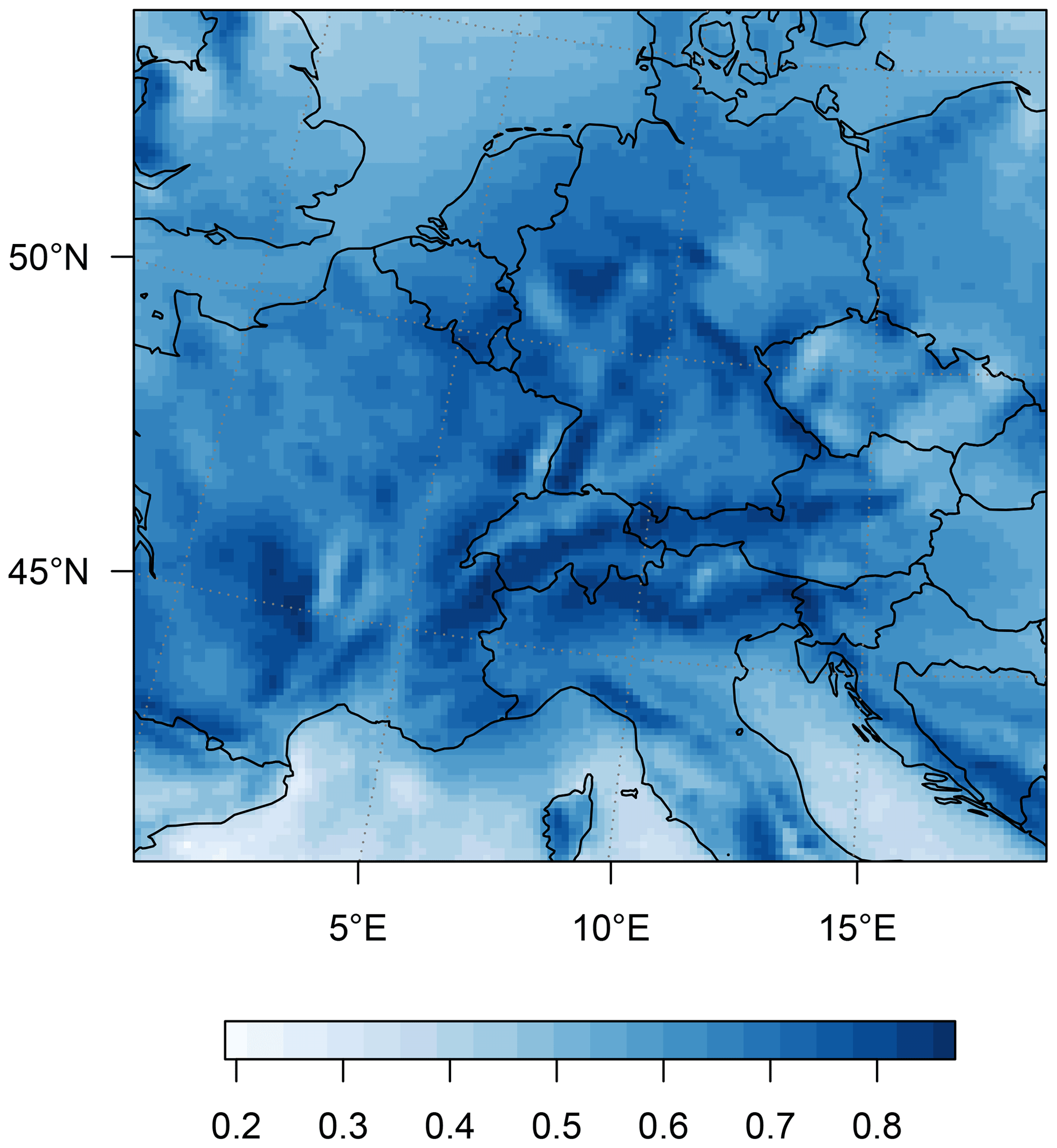
Figure B2Training 1955–2020: proportion of variance explained (R2) for each grid cell for the precipitation predictions.
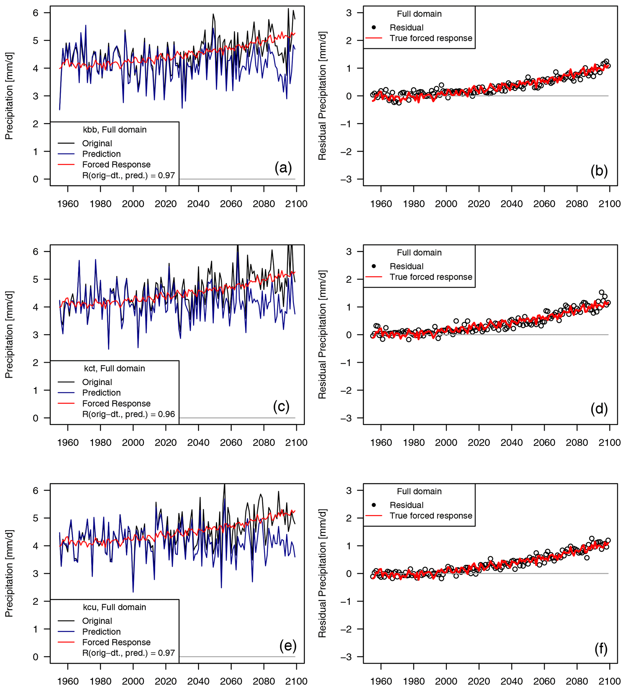
Figure B3Dynamical adjustment of the full domain (land grid cells only) but training only based on 1955–2020. (a, c, e) Seasonal precipitation totals simulated by three members of the high-resolution RCM in black (a: “kbb”, c: “kct”, e: “kcu”), the predicted (“circulation-induced”) component for three “holdout” ensemble members (blue), and the forced response (average across all 50 members, red). (b, d, f) Residuals from the prediction (black dots) and the forced response (red).
B1 Training on the time period 1955–2020
We train on the shorter period from 1955–2020 (as opposed to 1955–2070), using the same nine ensemble members as described in the main text. This corresponds approximately to a 43 % reduction in training data, but more importantly, this restricts the training to a period with relatively modest precipitation change. We then reproduce the analysis with this model trained on (i) this shorter time period and (ii) less data. We find that the MSE and R2 performance measures indicate very robust results with respect to these changes in the input data (see Figs. B1 and B2). Furthermore, the dynamical adjustment analysis based on the shorter training period reveals almost identical results as compared to the longer 1955–2070 training period. That is, the residual variability is much closer to the ensemble-mean forced response (see Fig. B3). This sensitivity analysis thus provides support that our method is robust to (i) a shorter time period and (ii) less training data points.
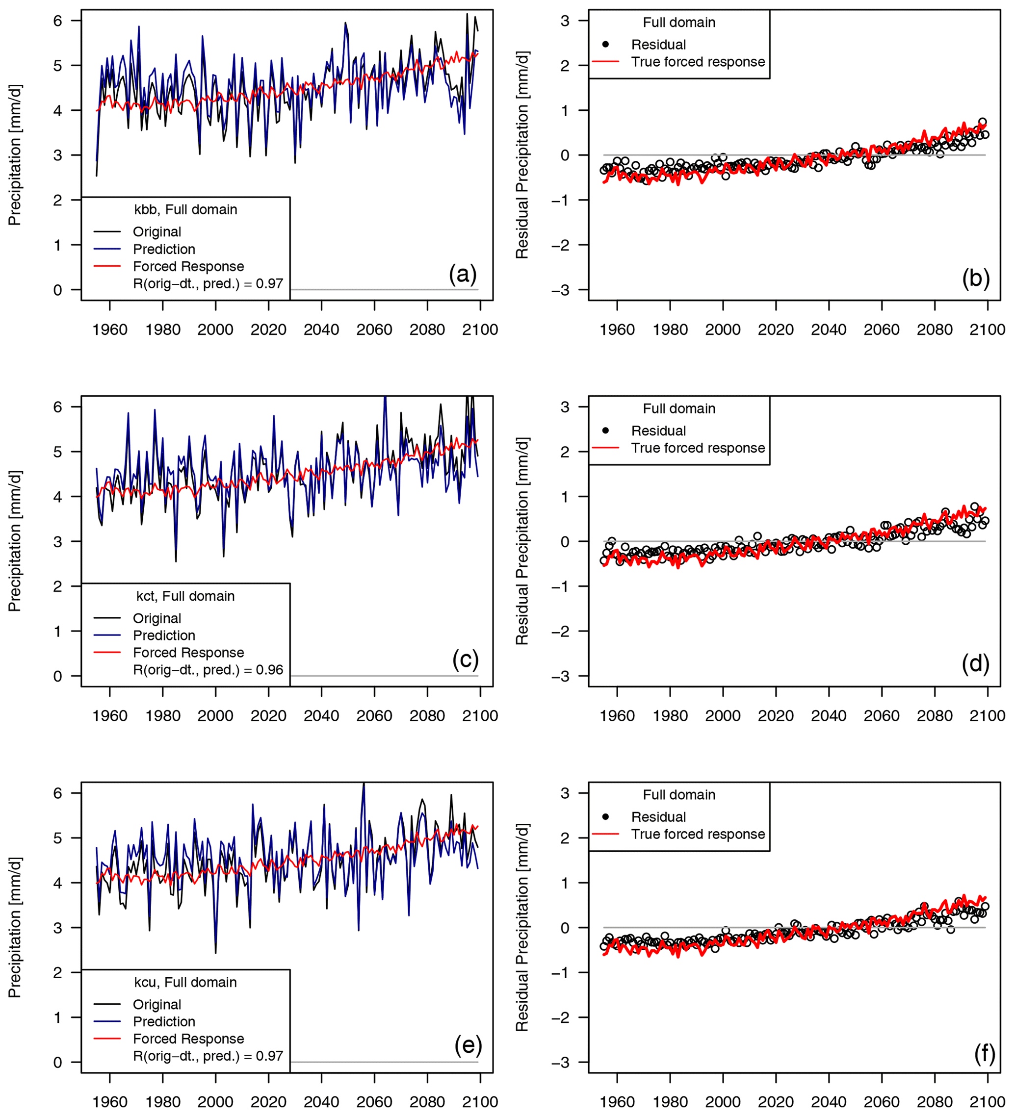
Figure B4Dynamical adjustment of the full domain (land grid cells only) but training only based on 1955–2020 and with precipitation detrended instead of SLP before model training and dynamical adjustment. (a, c, e) Seasonal precipitation totals simulated by three members of the high-resolution RCM in black (a: “kbb”, c: “kct”, e: “kcu”), the predicted (“circulation-induced”) component for three “holdout” ensemble members (blue) and the forced response (average across all 50 members, red). (b, d, f) Residuals from the prediction (black dots) and the forced response (red).
B2 Detrending precipitation
The question of whether and how to detrend prior to dynamical adjustment is open, somewhat subjective, and often discussed as an inherent subjective choice and uncertainty in dynamical adjustment papers (see, e.g. Deser et al., 2016; Lehner et al., 2017, 2018, for a discussion about trend removal). Here, in addition to the results presented above, we test an alternative simple detrending approach: SLP is not detrended, but we detrend precipitation using a simple LOESS smoother, fitted on the ensemble (seasonal) means at every location and subtracted from every day individually. (Furthermore, we here use the shorter 1955–2020 period for training the model.) For the dynamical adjustment analysis, we then compute the residuals based on the non-detrended precipitation data and our predictions (from the model trained on the detrended precipitation data; see Fig. B4). This analysis suggests that this approach to detrend precipitation is too simplistic since the residuals of the dynamical adjustment analysis underestimate forced changes (the ensemble mean) to some extent (Fig. B4). There are several possible reasons for this:
-
Precipitation change cannot be modelled by a single additive mean change across the whole distribution. For instance, precipitation change is known to increase the variance of the precipitation distribution (Pendergrass et al., 2017). Hence, by subtracting the estimated, seasonally averaged precipitation trend, we may have not fully removed the trend for wet days. Developing a more refined approach to remove the forced precipitation changes from daily data is non-trivial and beyond the scope of this work.
-
There may be some dynamically induced changes in precipitation, but it would be hard to evaluate this without any additional simulations where dynamical effects and thermodynamical effects could be separated.
Overall, we conclude that our simple SLP detrending (without detrending precipitation) is a useful approach for introducing LLAAEs as a versatile tool for dynamical adjustment, as demonstrated by the fact that the residuals of individual ensemble members after dynamical adjustment match the ensemble-mean trend of precipitation very well (e.g. Fig. 6). However, we acknowledge that considerations around whether and how to detrend the data prior to dynamical adjustment are crucial, especially for real-world applications (also see the discussion in Sect. 4.4).
The following results are based on temperature anomalies. In Fig. C1, we show examples from the holdout ensemble “kbb” of (i) original temperature fields Y (left column), (ii) reconstructions (centre column), and (iii) predictions (right column). The reconstruction quality, i.e. the similarity between the left and the centre column, is quite high, even though not all fine details are reproduced. For dynamical adjustment, we use the residuals, which are computed as the difference between the original fields (left column) and the predictions (right column). The predictions are computed using the linear model h and the decoder d with SLP time series as input. As can be seen, the proposed model yields spatially coherent predictions and explains a large proportion of the variance of Y.
Figure C2 shows the grid-cell-wise MSE, and Fig. C3 shows the R2 statistics for the holdout ensemble “kbb”.
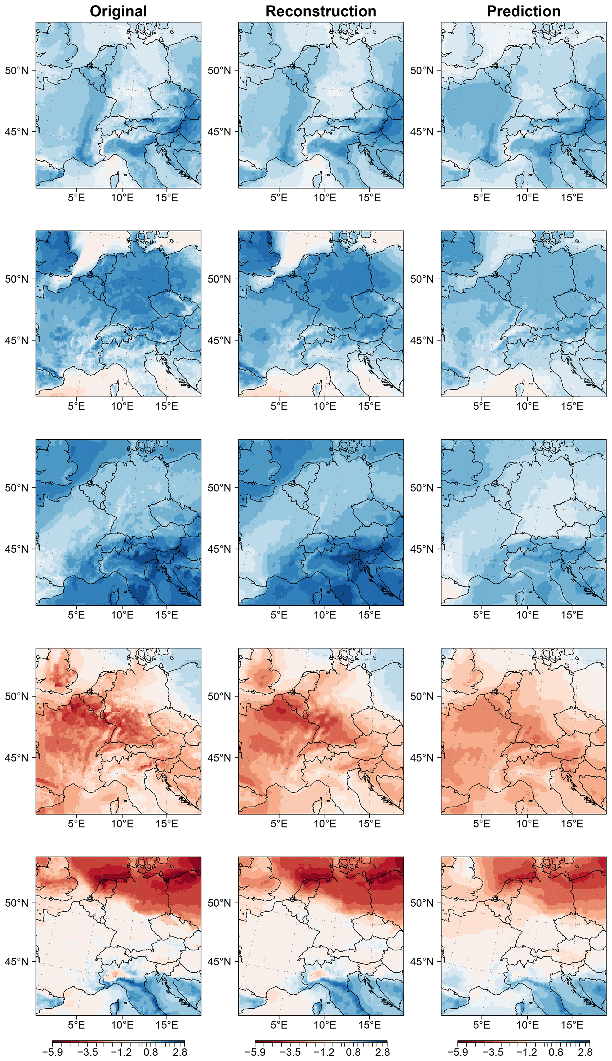
Figure C1Temperature anomalies. Examples of (i) original temperature fields Y (left column), (ii) reconstructions (centre column), and (iii) predictions (right column).
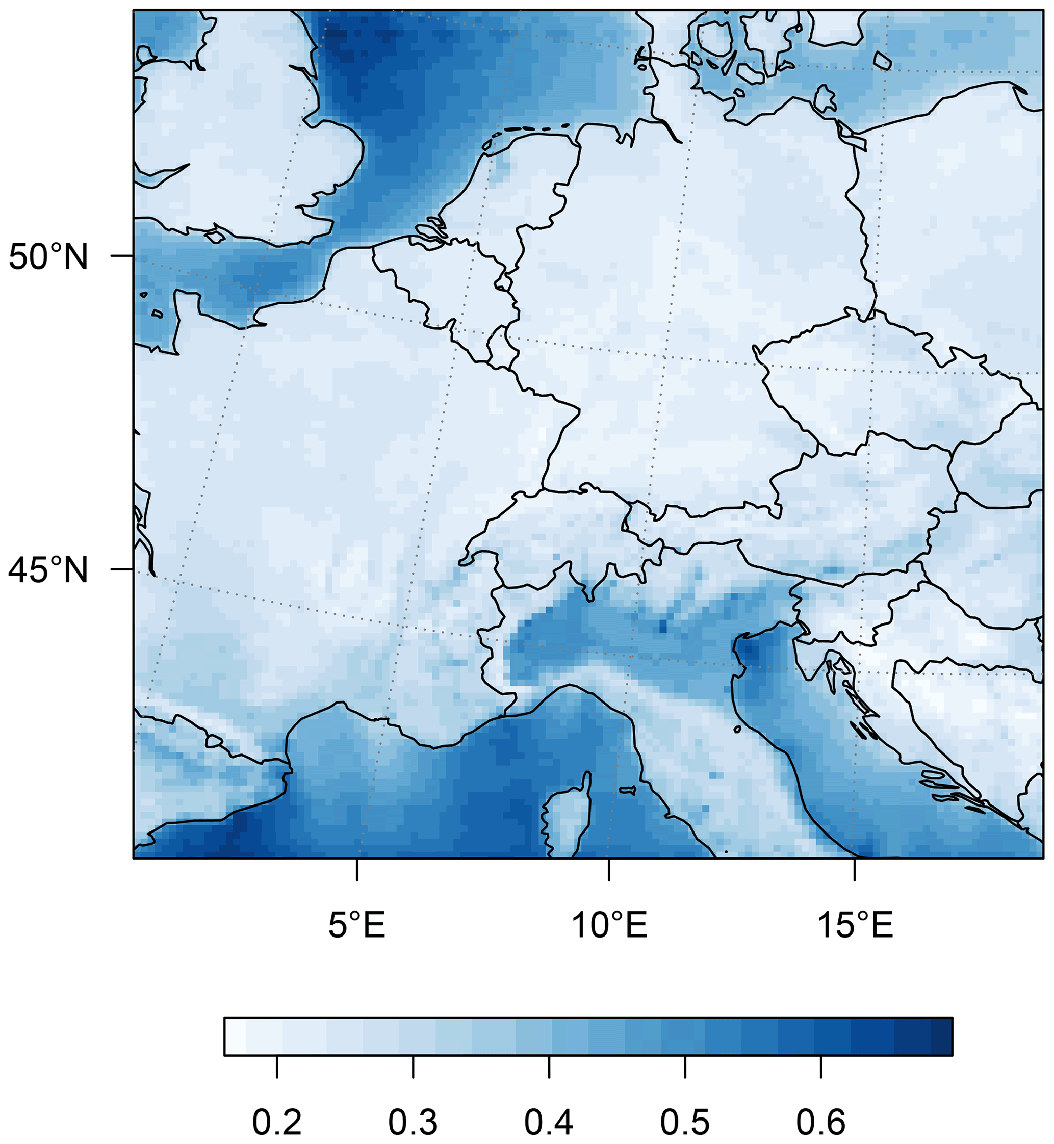
Figure C2Temperature anomalies. MSE for each grid cell for the temperature predictions.
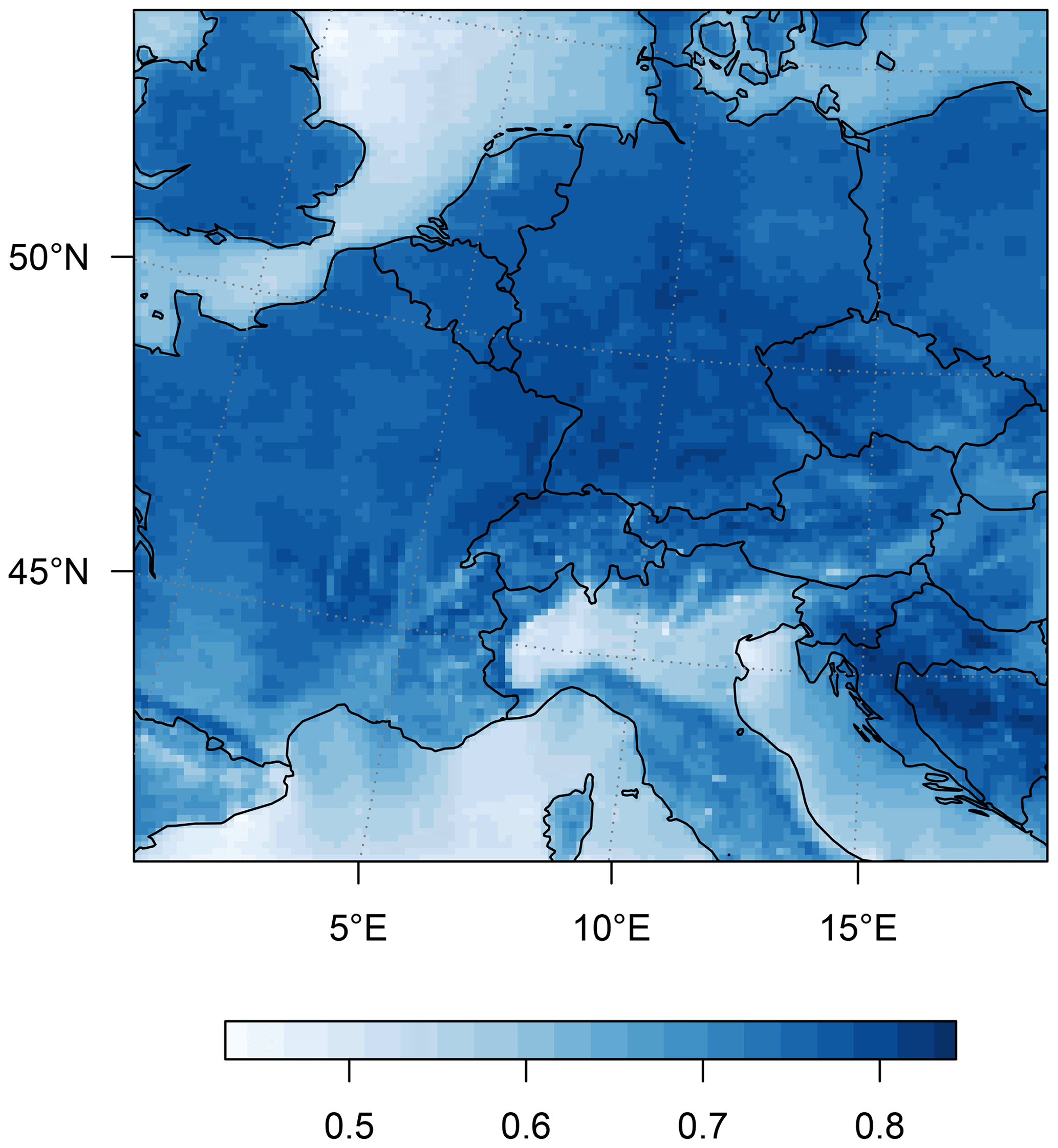
Figure C3Temperature anomalies. Proportion of variance explained (R2) for each grid cell for the temperature predictions.
The Latent Linear Adjustment Autoencoder model is free and open source. It is distributed under the MIT software license which allows unrestricted use. The source code is available at the following GitHub repository: https://github.com/christinaheinze/latent-linear-adjustment-autoencoders. A snapshot of the source code used to generate the results presented in this manuscript is available at https://doi.org/10.5281/zenodo.3957494 (Heinze-Deml, 2020a). The pretrained models can be obtained from https://doi.org/10.5281/zenodo.3950044 (Heinze-Deml, 2020c). Finally, the input data are available at https://doi.org/10.5281/zenodo.3949747 (Heinze-Deml, 2020b).
CH and NM conceptualized the Latent Linear Adjustment Autoencoder. CH, SS, and NM conceptualized the climate applications with support from AP and FL. CH, SS, and NM developed the methodology. CH did the formal analysis. CH and SS did the investigation and visualization. CH and SS wrote the original draft. CH, SS, AP, and NM reviewed and edited it.
The authors declare that they have no conflict of interest.
Publisher’s note: Copernicus Publications remains neutral with regard to jurisdictional claims in published maps and institutional affiliations.
We thank Raul Wood and Martin Leduc for providing the climate model simulations. The production of ClimEx was funded within the ClimEx project by the Bavarian State Ministry for the Environment and Consumer Protection. The CRCM5 was developed by the ESCER centre of Université du Québec à Montréal (UQAM; https://escer.uqam.ca/, last access: 10 August 2021) in collaboration with Environment and Climate Change Canada. We acknowledge Environment and Climate Change Canada's Canadian Centre for Climate Modelling and Analysis for executing and making available the CanESM2 Large Ensemble simulations used in this study, and the Canadian Sea Ice and Snow Evolution Network for proposing the simulations. Computations with the CRCM5 for the ClimEx project were made on the SuperMUC supercomputer at the Leibniz Supercomputing Centre (LRZ) of the Bavarian Academy of Sciences and Humanities. The operation of this supercomputer is funded via the Gauss Centre for Supercomputing (GCS) by the German Federal Ministry of Education and Research and the Bavarian State Ministry of Education, Science and the Arts. Furthermore, we would like to thank Ségolène Berthou and one anonymous referee for their helpful comments on an earlier version of the manuscript.
This material is based in part upon work supported by the National Center for Atmospheric Research, which is a major facility sponsored by the National Science Foundation (NSF) under cooperative agreement no. 1947282, and by the Regional and Global Model Analysis (RGMA) component of the Earth and Environmental System Modeling Program of the US Department of Energy's Office of Biological & Environmental Research (BER) via NSF IA 1844590. Sebastian Sippel acknowledges funding provided by the Swiss Data Science Centre within the project “Data Science-informed attribution of changes in the Hydrological cycle” (DASH, ID C17-01). Flavio Lehner has been supported by the Swiss National Science Foundation (grant no. PZ00P2_174128).
This paper was edited by Gerd A. Folberth and reviewed by Ségolène Berthou and one anonymous referee.
Allen, M. R. and Ingram, W. J.: Constraints on future changes in climate and the hydrologic cycle, Nature, 419, 228–232, 2002. a
Arora, V., Scinocca, J., Boer, G., Christian, J., Denman, K., Flato, G., Kharin, V., Lee, W., and Merryfield, W.: Carbon emission limits required to satisfy future representative concentration pathways of greenhouse gases, Geophys. Res. Lett., 38, L05805, https://doi.org/10.1029/2010GL046270, 2011. a
Beusch, L., Gudmundsson, L., and Seneviratne, S. I.: Emulating Earth system model temperatures with MESMER: from global mean temperature trajectories to grid-point-level realizations on land, Earth Syst. Dynam., 11, 139–159, https://doi.org/10.5194/esd-11-139-2020, 2020. a
Brogli, R., Sørland, S. L., Kröner, N., and Schär, C.: Causes of future Mediterranean precipitation decline depend on the season, Environ. Res. Lett., 14, 114017, https://doi.org/10.1088/1748-9326/ab4438, 2019. a
Castruccio, S., McInerney, D. J., Stein, M. L., Liu Crouch, F., Jacob, R. L., and Moyer, E. J.: Statistical emulation of climate model projections based on precomputed GCM runs, J. Climate, 27, 1829–1844, 2014. a
Deser, C., Knutti, R., Solomon, S., and Phillips, A. S.: Communication of the role of natural variability in future North American climate, Nat. Clim. Change, 2, 775–779, 2012. a, b
Deser, C., Terray, L., and Phillips, A. S.: Forced and internal components of winter air temperature trends over North America during the past 50 years: Mechanisms and implications, J. Climate, 29, 2237–2258, 2016. a, b, c, d, e, f, g, h, i
Deser, C., Lehner, F., Rodgers, K., Ault, T., Delworth, T., DiNezio, P., Fiore, A., Frankignoul, C., Fyfe, J., Horton, D. E., Kay, J. E., Knutti, R., Lovenduski, N. S., Marotzke, J., McKinnon, K. A., Minobe, S., Randerson, J., Screen, J. A., Simpson, I. R., and Ting, M.: Insights from Earth system model initial-condition large ensembles and future prospects, Nat. Clim. Change, 10, 277–286, 2020. a
Fereday, D., Chadwick, R., Knight, J., and Scaife, A. A.: Atmospheric dynamics is the largest source of uncertainty in future winter European rainfall, J. Climate, 31, 963–977, 2018. a, b, c, d
Guo, R., Deser, C., Terray, L., and Lehner, F.: Human influence on winter precipitation trends (1921–2015) over North America and Eurasia revealed by dynamical adjustment, Geophys. Res. Lett., 46, 3426–3434, 2019. a, b, c
He, K., Zhang, X., Ren, S., and Sun, J.: Deep residual learning for image recognition, in: Proceedings of the IEEE Conference on Computer Vision and Patern Recognition, 770–778, 2016. a
Heinze-Deml, C.: christinaheinze/latent-linear-adjustment- autoencoders: Latent Linear Adjustment autoencoders v1.0, Zenodo [code], https://doi.org/10.5281/zenodo.3957494, 2020a. a
Heinze-Deml, C.: Sample data of the CRCM5-LE for applications of the Linear Latent Adjustment autoencoder, Zenodo [data], https://doi.org/10.5281/zenodo.3949748, 2020b. a
Heinze-Deml, C.: Linear Latent Adjustment autoencoder: Pre-trained models, Zenodo [data], https://doi.org/10.5281/zenodo.3950045, 2020c. a
Held, I. M. and Soden, B. J.: Robust responses of the hydrological cycle to global warming, J. Climate, 19, 5686–5699, 2006. a
Jacob, D., Petersen, J., Eggert, B., Alias, A., Christensen, O. B., Bouwer, L. M., Braun, A., Colette, A., Déqué, M., Georgievski, G., Georgopoulou, E., Gobiet, A., Menut, L., Nikulin, G., Haensler, A., Hempelmann, N., Jones, C., Keuler, K., Kovats, S., Kröner, N., Kotlarski, S., Kriegsmann, A., Martin, E., van Meijgaard, E., Moseley, C., Pfeifer, S., Preuschmann, S., Radermacher, C., Radtke, K., Rechid, D., Rounsevell, M., Samuelsson, P., Somot, S., Soussana, J.-F., Teichmann, C., Valentini, R., Vautard, R., Weber, B., Yiou, P.: EURO-CORDEX: new high-resolution climate change projections for European impact research, Reg. Environ. Change, 14, 563–578, 2014. a, b
Jézéquel, A., Yiou, P., and Radanovics, S.: Role of circulation in European heatwaves using flow analogues, Clim. Dynam., 50, 1145–1159, https://doi.org/10.1007/s00382-017-3667-0, 2018. a
Kingma, D. P. and Ba, J.: Adam: A Method for Stochastic Optimization, in: 3rd International Conference on Learning Representations, San Diego, CA, USA, 7–9 May 2015. a, b
Kingma, D. P. and Welling, M.: Auto-Encoding Variational Bayes, in: 2nd International Conference on Learning Representations, Banff, AB, Canada, 14–16 April 2014. a, b, c
Kirchmeier-Young, M. C., Zwiers, F. W., and Gillett, N. P.: Attribution of extreme events in Arctic sea ice extent, J. Climate, 30, 553–571, 2017. a, b
Leduc, M., Mailhot, A., Frigon, A., Martel, J.-L., Ludwig, R., Brietzke, G. B., Giguère, M., Brissette, F., Turcotte, R., Braun, M., and Scinocca, J.: The ClimEx project: A 50-member ensemble of climate change projections at 12-km resolution over Europe and northeastern North America with the Canadian Regional Climate Model (CRCM5), J. Appl. Meteorol. Climatol., 58, 663–693, 2019. a, b, c, d, e
Lehner, F., Deser, C., and Terray, L.: Toward a new estimate of “time of emergence” of anthropogenic warming: Insights from dynamical adjustment and a large initial-condition model ensemble, J. Climate, 30, 7739–7756, 2017. a, b
Lehner, F., Deser, C., Simpson, I. R., and Terray, L.: Attributing the US Southwest's recent shift into drier conditions, Geophys. Res. Lett., 45, 6251–6261, 2018. a, b, c
Martynov, A., Laprise, R., Sushama, L., Winger, K., Šeparović, L., and Dugas, B.: Reanalysis-driven climate simulation over CORDEX North America domain using the Canadian Regional Climate Model, version 5: model performance evaluation, Clim. Dynam., 41, 2973–3005, 2013. a
Meinshausen, N.: Causality from a Distributional Robustness Point of View, in: 2018 IEEE Data Science Workshop, DSW 2018, Lausanne, Switzerland, 4–6 June 2018. a, b
Pendergrass, A. G.: What precipitation is extreme?, Science, 360, 1072–1073, 2018. a
Pendergrass, A. G., Knutti, R., Lehner, F., Deser, C., and Sanderson, B. M.: Precipitation variability increases in a warmer climate, Sci. Rep., 7, 17966, https://doi.org/10.1038/s41598-017-17966-y, 2017. a
Prein, A. F., Rasmussen, R. M., Ikeda, K., Liu, C., Clark, M. P., and Holland, G. J.: The future intensification of hourly precipitation extremes, Nat. Clim. Change, 7, 48–52, 2017. a, b
Rezende, D. J., Mohamed, S., and Wierstra, D.: Stochastic Backpropagation and Approximate Inference in Deep Generative Models, in: Proceedings of the 31st International Conference on Machine Learning, vol. 32, 1278–1286, 2014. a, b, c
Rothenhäusler, D., Meinshausen, N., Buhlmann, P., and Peters, J.: Anchor regression: heterogeneous data meets causality, arXiv [preprint], arXiv:1801.06229, 2018. a
Shepherd, T. G.: Atmospheric circulation as a source of uncertainty in climate change projections, Nat. Geosci., 7, 703–708, 2014. a, b
Shi, X. and Durran, D. R.: The Response of Orographic Precipitation over Idealized Midlatitude Mountains Due to Global Increases in CO2, J. Climate, 27, 3938–3956, https://doi.org/10.1175/JCLI-D-13-00460.1, 2014. a
Sippel, S., Meinshausen, N., Merrifield, A., Lehner, F., Pendergrass, A. G., Fischer, E., and Knutti, R.: Uncovering the Forced Climate Response from a Single Ensemble Member Using Statistical Learning, J. Climate, 32, 5677–5699, https://doi.org/10.1175/JCLI-D-18-0882.1, 2019. a, b, c, d
Smoliak, B. V., Wallace, J. M., Lin, P., and Fu, Q.: Dynamical adjustment of the Northern Hemisphere surface air temperature field: Methodology and application to observations, J. Climate, 28, 1613–1629, 2015. a, b, c, d
von Trentini, F., Leduc, M., and Ludwig, R.: Assessing natural variability in RCM signals: comparison of a multi model EURO-CORDEX ensemble with a 50-member single model large ensemble, Clim. Dynam., 53, 1963–1979, 2019. a
Wallace, J. M., Zhang, Y., and Renwick, J. A.: Dynamic contribution to hemispheric mean temperature trends, Science, 270, 780–783, 1995. a
Wallace, J. M., Fu, Q., Smoliak, B. V., Lin, P., and Johanson, C. M.: Simulated versus observed patterns of warming over the extratropical Northern Hemisphere continents during the cold season, P. Natl. Acad. Sci. USA, 109, 14337–14342, 2012. a
WCRP: CORDEX domains for model integrations, available at: https://cordex.org/domains/cordex-domain-description/ (last access: 10 August 2021), 2015. a
Yiou, P., Vautard, R., Naveau, P., and Cassou, C.: Inconsistency between atmospheric dynamics and temperatures during the exceptional 2006/2007 fall/winter and recent warming in Europe, Geophys. Res. Lett., 34, L21808, https://doi.org/10.1029/2007GL031981, 2007. a
Zorita, E., Hughes, J. P., Lettemaier, D. P., and von Storch, H.: Stochastic characterization of regional circulation patterns for climate model diagnosis and estimation of local precipitation, J. Climate, 8, 1023–1042, 1995. a
- Abstract
- Introduction
- Dynamical adjustment using statistical learning
- Data and evaluation
- Results and discussion
- Conclusion and future work
- Appendix A: Experimental details
- Appendix B: Additional experimental results for dynamical adjustment of daily precipitation
- Appendix C: Experimental results for dynamical adjustment of daily temperature
- Code and data availability
- Author contributions
- Competing interests
- Disclaimer
- Acknowledgements
- Financial support
- Review statement
- References