Comparison of source apportionment approaches and analysis of non-linearity in a real case model application

The response of particulate matter (PM) concentrations to emission reductions was analysed by assessing the results obtained with two different source apportionment approaches. The brute force (BF) method source impacts, computed at various emission reduction levels using two chemical transport models (CAMx and FARM), were compared with the contributions obtained with the tagged species (TS) approach (CAMx with the PSAT module). The study focused on the main sources of secondary inorganic aerosol precursors in the Po Valley (northern Italy): agriculture, road transport, industry and residential combustion. The interaction terms between different sources obtained from a factor decomposition analysis were used as indicators of non-linear PM₁₀ concentration responses to individual source emission reductions. Moreover, such interaction terms were analysed in light of the free ammonia / total nitrate gas ratio to determine the relationships between the chemical regime and the non-linearity at selected sites. The impacts of the different sources were not proportional to the emission reductions, and such non-linearity was most relevant for 100 % emission reduction levels compared with smaller reduction levels (50 % and 20 %). Such differences between emission reduction levels were connected to the extent to which they modify the chemical regime in the base case. Non-linearity was mainly associated with agriculture and the interaction of this source with road transport and, to a lesser extent, with industry. Actually, the mass concentrations of PM₁₀ allocated to agriculture by the TS and BF approaches were significantly different when a 100 % emission reduction was applied. However, in many situations the non-linearity in PM₁₀ annual average source allocation was negligible, and the TS and BF approaches provided comparable results. PM mass concentrations attributed to the same sources by TS and BF were highly comparable in terms of spatial patterns and quantification of the source allocation for industry, transport and residential combustion. The conclusions obtained in this study for PM₁₀ are also applicable to PM_2.5.

1 Introduction

Air pollution is the main environmental cause of premature death. Ambient air pollution caused 4.2 million deaths worldwide in 2016, contributing together with indoor pollution to 7.6 % of all deaths (WHO, 2018). Air pollution adverse health effects mainly occur as respiratory and cardiovascular diseases (WHO, 2016; EEA 2019). A key element for the design of effective air quality control strategies is the knowledge of the role of different emission sources in determining the ambient concentrations. This is usually referred to as source apportionment (SA) and involves the quantification of the influence of different human activities (e.g. transport, domestic heating, industry, agriculture) and geographical areas (e.g. local, urban, metropolitan areas, countries) to air pollution at a given location.

SA modelling studies involving secondary inorganic pollutants are generally based on chemistry transport models (Mircea et al., 2020). Two different SA approaches are commonly used to allocate the mass of pollutants to the different sources by means of chemical transport models.

• “Tagged species” (TS) quantifies the contribution of emission sources to the concentration of one pollutant at one given location by implementing algorithms to trace reactive tracers. SA studies based on tagging methods have been carried out at both European scale (e.g. Karamchandani et al., 2017; Manders et al., 2017) and urban scale (e.g. Pepe et al., 2019; Pültz et al., 2019).

• Brute force (BF or emission reduction impact) is a sensitivity analysis technique which estimates the change in pollutant concentration (impact) that results from a change in one or more emission sources. Sensitivity analysis techniques have been used to estimate the impact of different sources on pollution levels (e.g. Kiesewetter et al., 2015; Thunis et al., 2016; Van Dingenen et al., 2018).

Even though these approaches are often considered as two alternative SA methods, they actually pursue different objectives: TS aims to account for the mass transferred from the sources to the receptor in a specific area and time window, while BF is a sensitivity analysis technique used to estimate the response of the system to changes in emissions. For a detailed discussion, refer to Belis et al. (2020a), Mircea et al. (2020), and Thunis et al. (2019).

Clappier et al. (2017) applied the concept of factor decomposition developed by Stein and Alpert (1993) to investigate the differences between TS and BF using a theoretical example involving three sources. According to these authors, the change in concentration of a given pollutant due to the change in the emissions of three sources A, B and C (ΔC_ABC) can be described as follows:

$$\begin{array}{}\text{(1)}& \mathrm{\Delta }{C}_{\text{ABC}}=\mathrm{\Delta }{C}_{\mathrm{A}}+\mathrm{\Delta }{C}_{\mathrm{B}}+\mathrm{\Delta }{C}_{\mathrm{C}}+{\widehat{c}}_{\text{AB}}+{\widehat{c}}_{\text{AC}}+{\widehat{c}}_{\text{BC}}+{\widehat{c}}_{\text{ABC}},\end{array}$$

where ΔC_A, ΔC_B and ΔC_C are the variations of concentration of the studied pollutant due to the reduction in the single sources A, B and C, respectively, and those coming from the interactions between these sources denoted by the terms ${\widehat{c}}_{\text{AB}}$, ${\widehat{c}}_{\text{AC}}$, ${\widehat{c}}_{\text{BC}}$ and ${\widehat{c}}_{\text{ABC}}$ (see Appendix A for details). The interaction terms ($\widehat{c}$) have the same units as the source impacts.

In the TS approach, the sum of the contributions of the various sources always matches the total pollutant concentration by design ($M_{\text{poll}}=M_{\mathrm{A}}+M_{\mathrm{B}}+M_{\mathrm{C}}$), while this may be not the case for the BF approach ($\mathrm{\Delta }{C}_{\text{ABC}}\ne \mathrm{\Delta }{C}_{\mathrm{A}}+\mathrm{\Delta }{C}_{\mathrm{B}}+\mathrm{\Delta }{C}_{\mathrm{C}}$) under certain circumstances (Belis et al., 2020a). The interaction terms in Eq. (1) measure the consistency between the sum of single emission sources with respect to the contemporary reduction in more than one source in BF, for three sources $\mathrm{\Delta }{C}_{\text{ABC}}-(\mathrm{\Delta }{C}_{\mathrm{A}}+\mathrm{\Delta }{C}_{\mathrm{B}}+\mathrm{\Delta }{C}_{\mathrm{C}})$, which is an indicator of the non-linearity in the response of the pollutant concentration to single-source reductions (impacts).

There are different situations that may contribute to generating non-linear responses when secondary pollutants' precursors are emitted by different sources. They are double counting, chemical regime limited by one precursor, competition between precursors, thermodynamic equilibrium between the secondary pollutant and its precursors, and compensation. A detailed explanation of each of them is provided in Appendix A.

In the analysis of a theoretical example with three sources (agriculture, industry and residential), Clappier et al. (2017) observed that strong non-linearity is associated with secondary inorganic aerosol (SIA, ammonium nitrate and ammonium sulfate) formation. However, this secondary aerosol may behave linearly or non-linearly depending on the circumstances, for instance, the intensity of the emission reduction, which imposes the need to quantify it for different emission reduction levels (ERLs) (see Sect. 3.2). Thunis et al. (2015) showed that for yearly average relationships between emission and concentration changes, linearity is often a realistic assumption and, consequently, TS and BF methods are expected to provide comparable results, as reported by Belis et al. (2020a). The abovementioned considerations suggest the need to monitor whether non-linearity is significant for a given study area and time window.

The objective of this study is to identify and quantify the factors leading to non-linear response of PM concentrations to source emission reductions in a real-world situation with significant PM concentrations. To that end, the influence on PM₁₀ concentration of various sources with different chemical profiles was calculated using both the BF approach with two different chemical transport models (CAMx and FARM) and the TS approach using one of these chemical-transport models (CAMx).

The results of the simulations were then used to

• compare TS contributions with BF impacts,

• analyse the geographical patterns,

• compute interaction terms (of the Stein and Alpert algebraic expression) for the studied sources, and

• compare the behaviour of various areas (urban, rural, etc.) with different chemical regimes.

In this study, the focus is on the non-linearity associated with SIA formation, with particular reference to ammonium nitrate (NH₄NO₃) and ammonium sulfate ((NH₄)₂SO₄). The possible non-linear behaviour of any other PM component (e.g. organics) is beyond the scope of this exercise.

2 Materials and methods

The Po Valley was selected for this study because of its high levels of particulate matter due to the high emissions of primary pollutants and precursors of SIA, whose high concentrations are also favoured by the stagnation of air masses during the coldest months of the year (Belis et al., 2011; Larsen et al., 2012).

The air quality simulations were performed with the CAMx (ENVIRON, 2016) and FARM (ARIANET, 2019) chemical transport models (CTMs). Both are open-source modelling systems for multi-scale integrated assessment of gaseous and particulate air pollution. Thanks to their variable spatial resolution, they are used for urban- to regional-scale applications and, simulating the atmospheric chemical reactions of the emitted precursors, they allow reconstruction of the formation of most of the secondary compounds, including the constituents of particulate matter. CAMx is widely used to assess the influence of pollution sources on air quality in a particular domain. The PM source apportionment technology (PSAT; Yarwood et al., 2004) implemented in CAMx offers the choice between several SA approaches, which allows users to easily compare e.g. TS versus BF methods for the estimation of source contributions to pollutant concentrations using the same model. In addition, the application of the BF method with FARM made it possible to show the structural behaviours that are less dependent on the specific model formulation and consequently to obtain results of more general value.

The application of such CTMs required the implementation of a comprehensive modelling system (e.g. Pepe et al., 2019), including specific tools aiming at creating the three main input categories: meteorological fields, emissions and boundary conditions.

Both modelling systems were applied for the reference year 2010 over northern Italy (Figs. S1 and S2 in the Supplement) considering a computational domain that covers a 580×400 km² region, with a 5 km grid step. For the meteorological model WRF (Skamarock et al., 2008) three nested grids were used, the largest one covering Europe and northern Africa and the innermost one corresponding to Italy and the Po Valley, respectively. The three meteorological domains have 45, 15, and 5 km grid resolution. For CTMs only the innermost WRF nested grid was used. Both CTMs were set up using the same input meteorological data and horizontal grid structure of WRF. The CTM vertical grid was defined by collapsing the 27 vertical layers used by WRF into 14 layers while keeping identical the layers up to 1 km above ground level; in particular, the first layer thickness was up to about 25 m from the ground like the corresponding WRF layer.

In CAMx, homogenous gas-phase reactions of nitrogen compounds and organic species were reproduced through the CB05 mechanism (Yarwood et al., 2005). The aerosol scheme was based on two static modes (coarse and fine). Secondary inorganic compound evolution was described by the thermodynamic model ISORROPIA (Nenes et al., 1998), while SOAP (ENVIRON, 2011) was used to describe secondary organic aerosol formation. Meteorological input data were provided by WRF and were completed by OMI satellite data (https://nasatoms.gsfc.nasa.gov, last access: 13 July 2021), including ozone vertical content and aerosol turbidity. Vertical turbulence coefficients (Kv) were computed using the O'Brien scheme (O'Brien, 1970) but adopting two different minimum Kv values for rural and urban areas so as to consider heat island phenomena and increased roughness of built areas.

FARM simulations were performed using the SAPRC-99 gas-phase chemical mechanism (Carter, 2000) and a three-mode aerosol scheme (Binkowski and Roselle, 2003) including microphysics, ISORROPIA for thermodynamic equilibrium of inorganic species and SORGAM (Schell et al., 2001) for secondary organic aerosol formation. Meteorological input from WRF was complemented by Kv computed using Lange (1989) parameterisation.

Emissions were derived from inventory data at three different levels: European Monitoring and Evaluation Programme data (EMEP, https://www.ceip.at/webdab-emission-database/emissions-as-used-in-emep-models, last access: 13 July 2021) available over a regular grid of 50×50 km² and ISPRA Italian national inventory data (http://www.sinanet.isprambiente.it/it/sia-ispra/inventaria/disaggregazione-dellinventario-nazionale-2015/view, last access: 13 July 2021), which provide a disaggregation by province. Moreover, regional inventory data based on the INEMAR methodology (INEMAR – ARPA Lombardia, 2015) provided detailed emission data at municipality level for the four administrative regions of Lombardy, Piedmont, Veneto and Emilia-Romagna.

Each emission inventory was processed to obtain the hourly time pattern of the emissions. For the CAMx simulations this was accomplished using the Sparse Matrix Operator for Kernel Emissions model (SMOKE v3.5) (UNC, 2013). Temporal disaggregation was based on monthly, daily and hourly profiles deduced by CHIMERE (INERIS, 2006) and EMEP models from the Institute of Energy Economics and the Rational Use of Energy (IER) project named GENEMIS (Pernigotti et al., 2013). Similar emission inventory processing was performed for FARM using the Emission Manager pre-processing system (ARIA Technologies and ARIANET, 2013).

Initial and boundary conditions were taken from a parent CAMx simulation covering the whole of Italy and driven by the MACC-II system (https://cordis.europa.eu/project/id/283576, last access: 14 July 2021) that provides 3D global concentration fields.

Table 1 Macro-sectors according to the EEA SNAP classification for emission inventories used to define air pollution sources in this study.

The CAMx modelling system was applied with the previously described setup in order to perform a TS run (with PSAT) and three sets of BF runs with 100 %, 50 % and 20 % emission reduction levels (ERLs), while FARM was used to produce two sets of BF runs with 50 % and 20 % ERLs. Due to the high number of runs needed to apply the Stein and Alpert decomposition, only a few sources were selected (Table 1). Originally, the study focused on the same system of three sources (AGR, IND, RES) as the study by Clappier et al. (2017). However, due to the small non-linearity associated with RES, the focus was then shifted to a ternary system including AGR, TRA and IND. In total, 41 runs were performed, keeping all inputs as the base case (BC), except for emissions that were modified according to the scheme reported in Table 2.

Table 2 Sets of simulations performed in this study to compute the factor decomposition (Stein and Alpert, 1993). Every set is named after the used CTM and ERL.

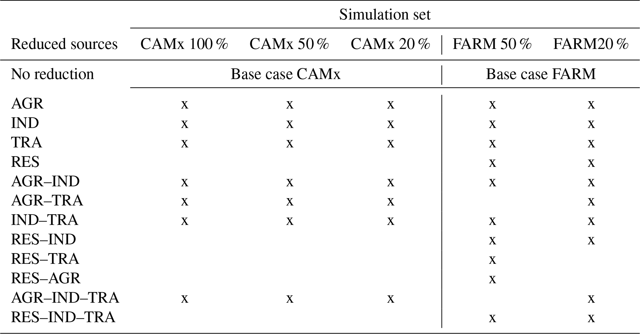
In this study, the interactions between sources AGR, TRA and IND are mainly analysed. Additional runs were executed using FARM at 50 % and 20 % ERLs to test also the impacts and interactions of RES with the previous ones.

3 Results and discussion

3.1 Comparison between source apportionment TS and BF approaches

The yearly average PM₁₀ concentrations in the CAMx and FARM base case runs are shown in Figs. S1 and S2. Figure 1 shows the relative contributions of the modelled PM₁₀ sources using the TS approach (CAMx-PSAT). The contributions of AGR are distributed across the entire Po Valley, with maximum levels in the centre and hotspots to the NW and SE. The IND contributions are highest to the south, SE and NE of the study area. The TRA contributions to PM₁₀ are highest in the main urban areas, in particular Milan and Turin, and along the main highways (e.g. A4 Turin–Venice). The highest contributions of all the other remaining sources (OTHER) are observed in the pre-Alpine area and in the Alpine valleys (including some areas in the Apennines), where the average PM₁₀ levels are lower than the Po Valley (Figs. S1 and S2) and RES is an important source (see below).

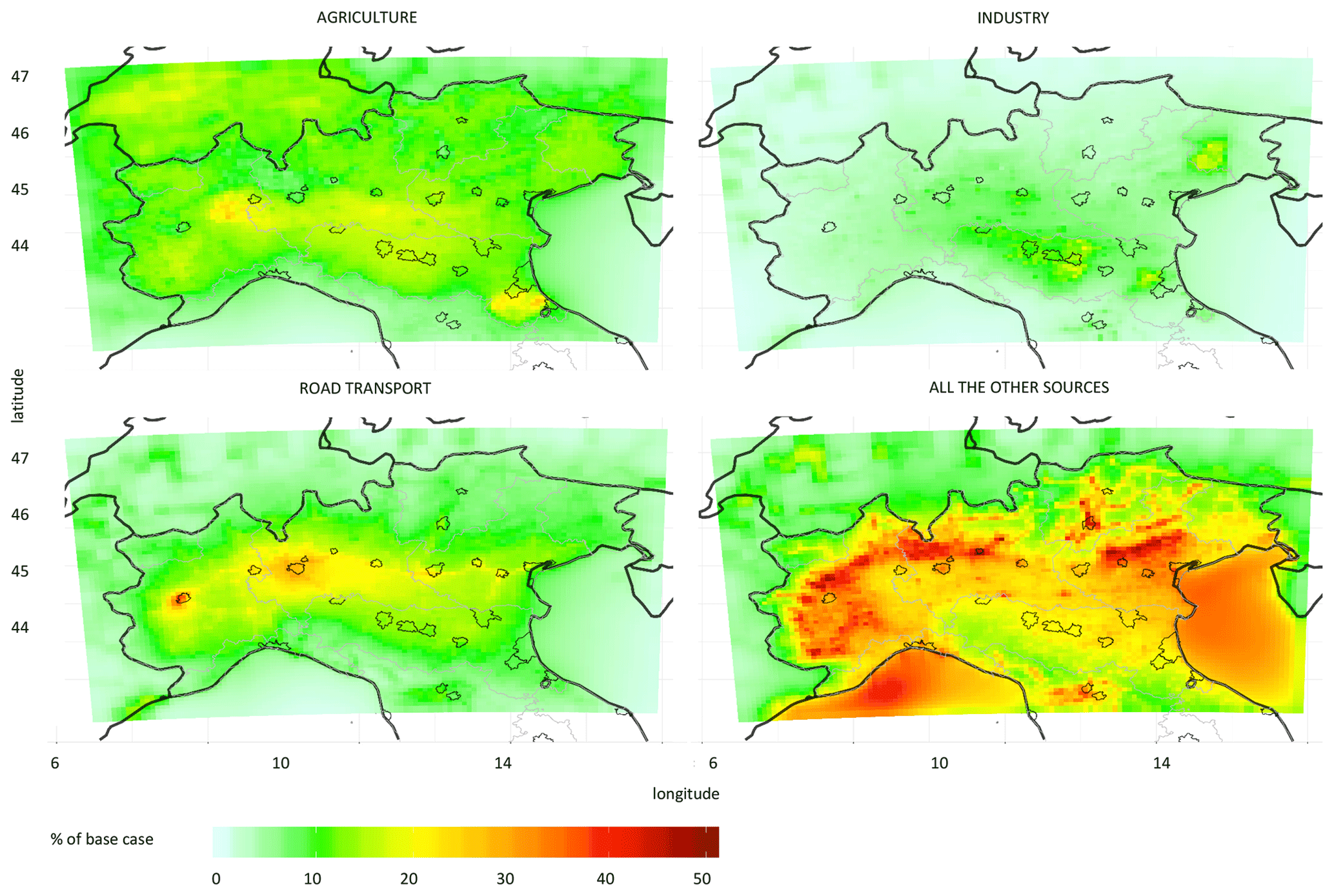
Figure 1 Annual contributions of the PM₁₀ sources over the Po Valley area according to the tagged species (TS) approach as computed by CAMx-PSAT. The grey lines indicate the boundaries of the regions and the polygons represent the municipal areas of the main cities.

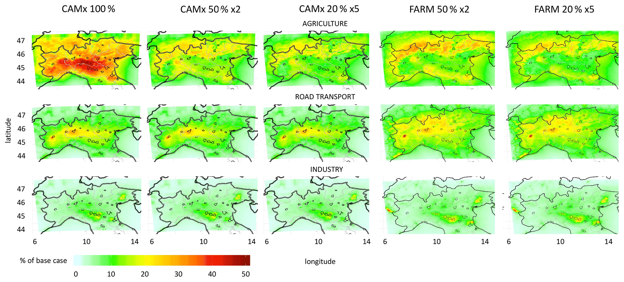
Figure 2 Annual average impacts of AGR, TRA and IND expressed as a percentage of the base case. From left to right: CAMx 100 %, 50 % and 20 % emission reduction levels and FARM 50 % and 20 % emission reduction levels. For a direct comparison of the linearity between the different ERLs, the impacts of 50 % and 20 % are multiplied by 2 and 5, respectively.

The annual average impacts of AGR, TRA and IND on PM₁₀ derived by the BF approach with CAMx and FARM for different emission reduction levels (ERLs) are shown in Fig. 2, while those of RES are shown in Fig. S3 in the Supplement. In a linear situation the impacts allocated to each source decrease proportionally to the intensity of the emission reduction ($\mathrm{\Delta }{C}_{\mathrm{100}\mathit{\%}}=\mathrm{2}\mathrm{\Delta }{C}_{\mathrm{50}\mathit{\%}}=\mathrm{5}\mathrm{\Delta }{C}_{\mathrm{20}\mathit{\%}}$). For that reason, the impacts at 100 % ERL can be compared directly with TS contributions, while those of 50 % and 20 % must be multiplied by factors 2 and 5, respectively. The linearity between different ERLs is discussed in Sect. 3.2. To facilitate the comparison between different models, impacts are expressed as a percentage of the base case in these figures. In Fig. 2, the highest impacts are those of AGR followed by TRA and IND. The outputs resulting from CAMx and FARM for 50 % and 20 % ERLs present similar levels and geographical patterns. Most of the highest impacts of AGR at 100 % ERL are observed in or near the areas of high NH₃ emissions (Fig. S4 in the Supplement), in which TS also points to high contributions of this source (Fig. 1). However, in these areas the BF impacts are nearly twice the TS contributions reported in Fig. 1 (see also Fig. 3, top left). Such high levels could be attributed to a near-double-counting effect which is dominant only at this ERL because the effect of a limited chemical regime cannot be observed at 100 % reduction (see Appendix A Sect. A2.2). At 50 % and 20 % ERLs the impacts are lower than 100 % ERL, because of the limited regime, and the highest ones are located in the mountainous areas (Alps and Apennines). Such a pattern is likely due to the low emissions of the SIA precursors (NH₃, NO_x and SO₂) (Fig. S4) and the modest base case PM₁₀ concentrations in these areas. For IND and TRA, the geographical patterns of BF are comparable to those of TS (Figs. 1 and 3 left) and do not vary significantly between the different ERLs, as discussed in Sect. 3.2. The only remark is that FARM presents higher TRA impacts in the subalpine areas compared to CAMx, irrespective of the SA approach used.

Figure 3 Scatter plots of the single grid cell annual average BF source impacts (CAMx and FARM) on PM₁₀ versus the TS contributions (CAMx–PSAT) for 100 %, 50 % (multiplied by 2) and 20 % (multiplied by 5) ERLs for AGR, TRA and IND. Dotted line: regression; red line: identity.

As shown in Fig. 3, the single grid cell annual averages of BF impacts on PM₁₀ by IND and TRA plotted versus the TS contributions are arranged on a line close to the identity, indicating that BF and TS approaches lead to similar results for these two sources. A similar behaviour is observed in all the ERLs even though the BF impacts estimated with FARM present a higher dispersion than those obtained with CAMx. Such a closer relationship between TS (CAMx-PSAT) and CAMx BF results is likely a consequence of both being results of the same model. By contrast, the impacts of AGR on PM₁₀ at 100 % ERL are more than twice the TS contributions in most grid cells, which is due to the much greater AGR BF impacts on sulfate and nitrate than TS contributions at this ERL (Figs. S5 and S6 in the Supplement, respectively). Such non-linear behaviour is associated with a situation near to double counting, which results in negative interaction terms, and for nitrate, also near to the NH₄NO₃ equilibrium, since both effects lead to BF impacts higher than TS contributions (Appendix A).

Despite the comparable range of BF impacts and TS contributions of AGR on PM₁₀ at 50 % and 20 % ERLs (Fig. 3), there is a considerable dispersion around the regression line (R² between 0.65 and 0.72), indicating spatial heterogeneity. In addition, impacts at 20 % ERL present a slightly lower slope with respect to TS contributions than those at 50 % ERL. Also, AGR BF impacts on nitrate present non-linear high values at 50 % and 20 % ERLs, which are however compensated for by ammonium impacts which are much lower than TS contributions (Figs. S6 and S7 in the Supplement, respectively). The greater difference observed between TS and BF at 100 % ERL for AGR compared to TRA and IND is in part due to AGR being the only significant source of NH₃ in the domain. Consequently, a 100 % reduction in AGR implies an almost complete abatement of NH₃, while 100 % reduction in TRA or IND does not reduce NO_x and SO₂ emissions completely (compensation effect). The reported differences between AGR TS contributions and BF impacts on PM₁₀ concentrations are due to the way in which the two approaches allocate ammonium, nitrate and sulfate to this source. TS allocates secondary constituents according to the mass of precursors deriving from each source (Mircea et al., 2020; Yarwood et al., 2004). Therefore, for TS the contribution of AGR is close to the mass fraction of ammonium in PM₁₀, and very little nitrate and sulfate is allocated to this source, since SO₂ and NO_x emissions from AGR are small compared to those from IND and TRA. By contrast, BF allocates these constituents on the basis of the amount of NH₄NO₃ and/or (NH₄)₂SO₄, which is not formed when such sources are reduced. Consequently, considerable nitrate and sulfate are allocated to AGR by BF, even though they are not physically emitted by this source, because there is no formation of NH₄NO₃ and/or (NH₄)₂SO₄ in the absence of NH₃ emissions from AGR.

Even in the cases where BF impacts and TS contributions to PM₁₀ are linear and close to identity, PM₁₀ constituents may not behave in the same way. Sometimes, the linearity observed in PM₁₀ is the result of a compensation between constituents for which BF impacts>TS contributions and others for which BF impacts<TS contributions. A good example is TRA, whose annual BF impacts on PM₁₀ are aligned with TS contributions (Fig. 3). However, the ammonium impacts from this source are highly non-linear and larger than TS contributions (Fig. S7), sulfate impacts are quite non-linear and can be either larger or smaller compared to TS contributions (Fig. S5), while nitrate impacts are rather linear and slightly lower than TS contributions (Fig. S6). A similar situation is observed for nitrate and ammonium impacts from IND, with the difference that in this case sulfate, a component for which this source is dominant, is rather linear.

The non-linearity between TS and BF source apportionment of PM₁₀ secondary inorganic constituents observed in Figs. S5–S7 occurs when the BF and TS approaches do not allocate these compounds to the same sources. For instance, high non-linearity is observed for BF impacts of TRA and IND on ammonium because it is emitted almost exclusively by AGR, while BF methods allocate impacts on ammonium to TRA and IND due to the atmospheric reactions between NH₃ and HNO₃ or H₂SO₄, which are mainly emitted from TRA and IND, respectively. A similar situation is observed for AGR impacts on sulfate and nitrate. TS allocates a negligible share of these compounds to AGR (proportional to SO₂ and NO_x emissions from AGR only), while the BF method allocates them to this source proportionally to the (NH₄)₂SO₄ and NH₄NO₃ concentration variations, respectively.

The analysis of the impacts reported in this section clearly points to AGR as the source mostly associated with the non-linear response of BF impacts with respect to TS.

3.2 Non-linearity between different ERLs

In this section the connection between the magnitude of the emission reduction and the BF source impacts on PM₁₀ is analysed more in detail. The scatter plots in Fig. 4 depict the relationships between BF impacts at different ERLs for every source and model. IND is the source for which the similarity between the different ERLs is the highest with regression slopes and R² between impacts calculated for the three ERLs of CAMx and the two of FARM near unity. Although the regressions between TRA impacts are also linear, the 50 % ERL impacts are ca. 8 % lower and 20 % ERL ca. 12 % lower than those obtained with 100 % ERL using the same model. The impacts at 50 % and 20 % ERLs are well correlated, and the latter are less than 5 % below the former for both CAMx and FARM values. For AGR the relationship between the impacts calculated for both 50 % and 20 % ERLs are clearly non-linear when compared to 100 % ERL. In the latter impacts are 3 or 4 times higher than the former two, especially for mid to high impacts. By comparison, the relationship between impacts at 50 % and 20 % ERLs is closer to linearity (R²=0.99), with the latter leading to 18 %–20 % lower impacts than the former. The results shown in Fig. 4 confirm that AGR is the source presenting the most serious non-linearity among those emitting SIA precursors (see Sect. 3.1). In addition, the analysis indicates that also for TRA the impacts of the different ERLs are not fully equivalent.

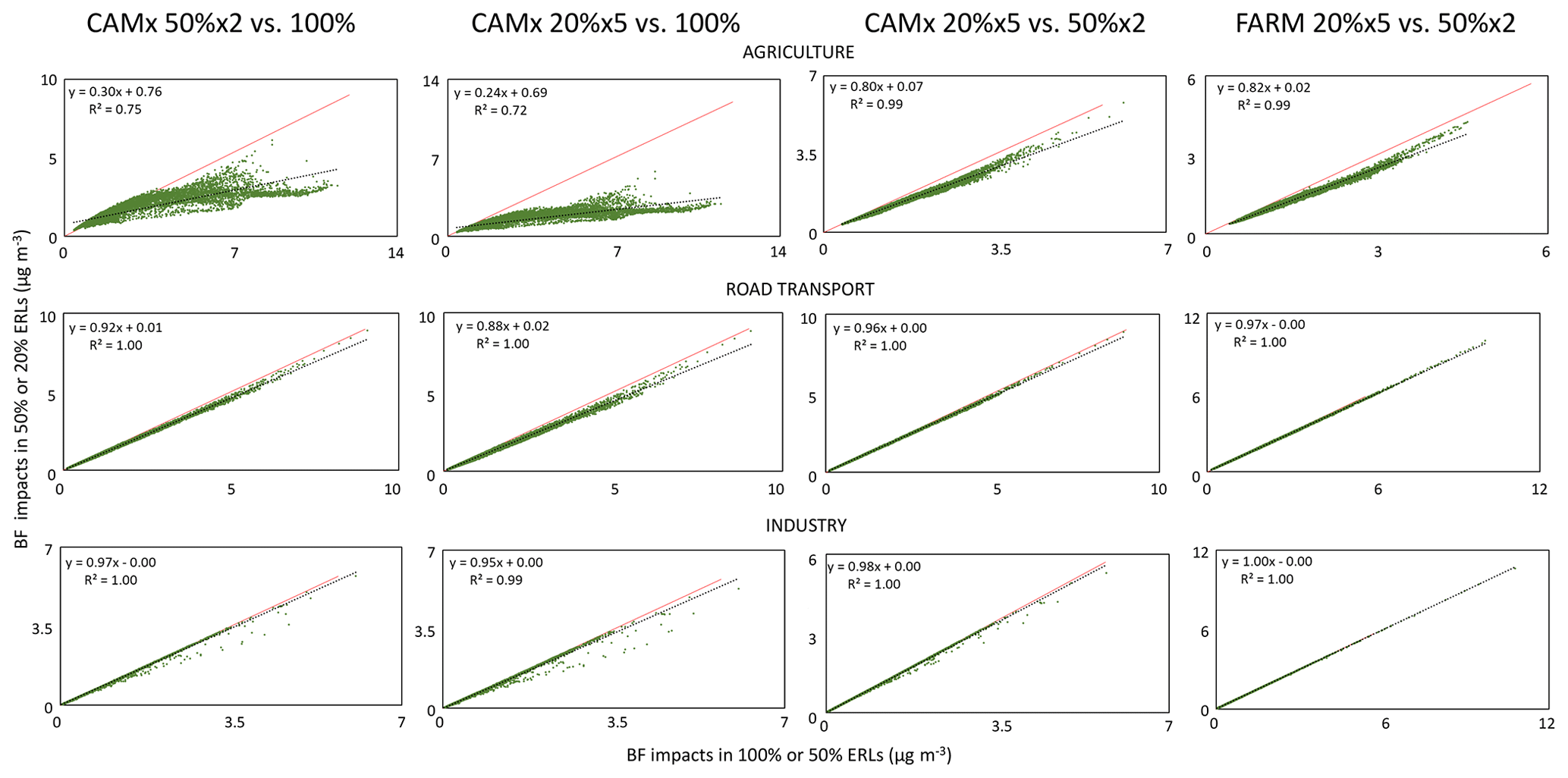
Figure 4 Scatter plots of the single grid cell BF source impacts (CAMx and FARM) on PM₁₀ between 100 %, 50 % (multiplied by 2) and 20 % (multiplied by 5) ERLs for AGR, TRA and IND. Dotted line: regression; red line: identity.

The large differences in AGR impacts on PM₁₀ between 100 % and the other ERLs are likely explained by two reasons. Firstly, turning off AGR 100 % systematically shifts the system into a different chemical regime, while this is not the case for the other sources, and secondly, the influence of limiting precursors (leading to less than double counting and consequently less BF overestimation with respect to TS) is not expressed at 100 % ERL (Appendix A Sect. A2.2). The differences between 50 % and 20 % ERLs could be explained by the way in which limited chemical regimes interact with the reduction in emissions. Since the non-linearity associated with limited chemical regimes appears only when the emission reduction causes a drop in concentrations higher than the excess of the non-limiting precursor (Appendix A), the chance of such non-linearity influencing source impacts is proportional to the emission reduction. However, the relatively small differences observed between 50 % and 20 % ERLs are likely due to the smoothing effect of the NH₄NO₃ equilibrium with respect to the non-linearity caused by a limited chemical regime because such equilibrium leads PM₁₀ concentrations to change even when the non-limiting precursor emission reduction is lower than the excess (Appendix A Fig. A1).

3.3 Interaction terms

In Fig. 5 the annual average interaction terms ($\widehat{c}$) of the factor decomposition, which are used in this study as indicators of the impact's non-linearity, are mapped. The binary interaction terms are, in general, of higher magnitude than the ternary interaction terms. The most negative interaction terms (indicating BF>TS) are observed in 100 % ERL for the contemporary reduction in AGR and TRA in the rural areas located to the north of the Po Valley where NH₃ is in excess, while the interaction terms are less negative in the main urban areas, where NH₃ is a limiting factor. When AGR and IND are both reduced by 100 %, the most negative interaction terms are observed in the industrial districts around the main cities to the south of the Po Valley and to a lesser extent in the rural areas in the central Po Valley. By contrast, positive interaction terms are observed for the IND–TRA binary reduction due to the competition between HNO₃ and H₂SO₄ that leads to an increase in the PM formation when SO₂ emissions (mainly industrial) are reduced in the presence of NO_x (deriving mainly from road transport). Such maximum positive interactions are observed in vast areas of the central Po Valley. A similar geographical pattern of the interaction terms is observed for 50 % and 20 % ERL (Figs. S8 and S9 in the Supplement, respectively), with the magnitude of the interaction decreasing with the emission reduction.

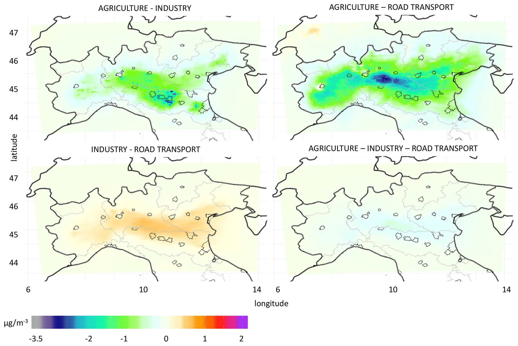
Figure 5 Map of the binary and ternary interaction terms of the PM₁₀ factor decomposition for AGR, IND and TRA in the CAMx BF 100 % scenarios.

A similar analysis was carried with FARM at 50 % ERLs for residential heating (Fig. S10 in the Supplement), and the resulting interaction terms were very low compared with those of the other sources at the same ERL. The explanation is that despite the considerable contribution of this source to PM₁₀, its origin is mainly primary with a high non-reactive carbonaceous fraction (Piazzalunga et al., 2011), and therefore the impact on the secondary inorganic aerosol is limited.

The values of the interaction terms depend on the pollutant concentration. In order to define when $\widehat{c}$ is significantly different from zero, and consequently when the non-linearity is not negligible, the absolute value $\left|\mathrm{0.5}\right|$ % BC is proposed. Such an arbitrary threshold was defined to highlight the interactions that according to the analysis of the impacts presented in the previous sections are associated with evident non-linear situations (e.g. AGR–TRA). In Figs. S11 and S12 in the Supplement are reported the maps of the interaction terms expressed as a percentage of the base case for 100 % and 50 % ERLs, respectively. According to the proposed threshold, at 100 % ERL most of the Po Valley falls in the area where non-linearity is measurable for all the binary and ternary interactions. At 50 % ERL, the non-linearity of the binary interactions AGR–IND are measurable in industrial districts located to the SW and NW of the Po Valley, including the industrial areas to the NW of Milan. The non-linearity associated with the interaction AGR–TRA is not negligible in the entire Po Valley and also in the Alpine areas, probably due to the low PM₁₀ levels of the latter. The binary interaction IND–TRA exceeds the threshold only in the central area of the Po Valley and in a hotspot to the NW of Milan. The ternary interaction is below the threshold for the entire domain. For 20 % ERL (not shown), all the interactions are negligible according to CAMx, while FARM provides a pattern comparable to 50 % ERL.

3.4 Analysis of chemical regimes

A more in-depth analysis of the relationships between the chemical regime and the interaction terms was accomplished in three selected sites with different source emission set up (their position is shown in Fig. S1). A rural location at the border between the provinces of Cremona and Brescia (CR_P) was selected because of the high NH₃ emissions, while the local NO_x and SO₂ emissions are very limited. The site of Milan (MI) was selected because it is representative of a typical urban situation with high NO_x concentrations deriving from road transport emissions. The NH₃ emissions in this site are very limited and are associated with road transport, while SO₂ emissions are also low and derive in part from the energy production. The third site is an industrial area in the province of Ravenna (RA_P) located in the south-eastern Po Valley. In this location, there are considerable SO₂ emissions from industry, which also release NO_x, and moderate NH₃ emissions from the agricultural sector. In order to define the chemical regime in each base case (CAMx and FARM) and each of the simulations including binary or ternary interactions, the gas ratio (GR) proposed by Ansari and Pandis (1998) was used:

$$\begin{array}{}\text{(2)}& \text{GR}=\left(\right[{\mathrm{NH}}_{\mathrm{3}}]+[{\mathrm{NH}}_{\mathrm{4}}^{+}]-\mathrm{2}\left[{\mathrm{SO}}_{\mathrm{4}}^{\mathrm{2}-}\right])/\left(\right[{\mathrm{HNO}}_{\mathrm{3}}]+[{\mathrm{NO}}_{\mathrm{3}}^{-}\left]\right),\end{array}$$

where concentrations are nmol m⁻³ or in nmol mol of air (ppb).

The GR value defines three different chemical regimes:

• (a)

  GR>1, in which NH₄NO₃ formation is limited by the availability of HNO₃,

• (b)

  $\mathrm{0}<\text{GR}<\mathrm{1}$, in which NH₄NO₃ formation is limited by the availability of NH₃, and

• (c)

  GR<0, in which NH₄NO₃ formation is inhibited by H₂SO₄.

The plots in Fig. 6 display for each scenario the magnitude of the changes in the chemical regime with respect to the base case and the relationship between such changes and the interaction terms (expressed as a percentage of the PM yearly mean concentrations). Each plot is divided into zones defined by the combination of the GR thresholds and the threshold proposed in this study for the interaction terms ($\widehat{c}>\left|\mathrm{0.5}\mathit{\%}\text{BC}\right|$) as an indicator of non-negligible non-linearity in the mass concentration allocated to sources with respect to the PM mass concentration.

Figure 6 Plot of the interaction terms ($\widehat{c}$), expressed as a percentage of the base case (BC), in three selected sites with different chemical regimes versus the gas ratio (Ansari and Pandis, 1998). (a) CR_P: Cremona province, (b) MI: Milan and (c) RA_P: Ravenna province. C: CAMx and F: FARM. 10, 5 and 2 indicate 100 %, 50 % and 20 % ERLs, respectively. A: agriculture, I: industry and T: transport. White background indicates negligible interaction terms.

A common feature of all three sites is that the higher the ERL, the higher the difference between the GR of the scenarios and the one of the base case providing evidence about the extent to which the emission reductions alter the original conditions. The points representing simulations in which AGR is reduced sit to the left of their respective base case. The scenarios with 100 % ERL often lead to changes in the chemical regime and to the highest absolute interaction terms. On the other hand, 50 % and 20 % ERLs lead, in general, to $\widehat{c}$ values closer to zero than 100 % ERL, indicating lower or negligible non-linearity (located in the white background area). All interactions IND–TRA give rise to $\widehat{c}\text{values}\ge \mathrm{0}$, consistent with the competition effect (Appendix A Sect. A2.3). In CR_P and RA_P such simulations lead to increase in GR (data points in Fig. 6a and c are placed to the right of their base case), while in MI they lead to null or slightly negative changes in GR (data points are located to the left of the base case in Fig. 6b). This behaviour indicates that the simultaneous reduction in IND and TRA leads to a higher impact of ammonia+nitric acid on GR compared to the one of sulfate, in the three sites.

In CR_P the base cases of CAMx and FARM represent a HNO₃-limited chemical regime for NH₄NO₃ formation, in line with the rural character of this area (Fig. 6a). All scenarios where AGR is reduced lead to a decrease in GR (points located to the left of the corresponding base case), indicating a loosening of the HNO₃ limitation, while all those in which AGR is not reduced lead to an increase in GR (points located to the right of the corresponding base case), indicating a stronger HNO₃ limitation. Sizeable negative $\widehat{c}$ are observed in scenarios reducing AGR 100 %, likely associated with the shift towards a NH₃-limited regime when AGR, the only significant source of this precursor, is turned off. The described situation is reflected by the points representing the interaction terms AGR–IND (C10AI), AGR–TRA (C10AT) and AGR–IND–TRA (C10AIT) of 100 % ERL located in the bottom left of Fig. 6a. The only 100 % ERL scenario that does not lead to a chemical regime change is the contemporary reduction in IND and TRA (C10IT). It also leads to positive interaction terms resulting from the competition between HNO₃ and H₂SO₄. In this case, the abatement of SO₂ emissions leads to a reduced availability of H₂SO₄, which is replaced in the reaction with NH₃ by HNO₃, the latter deriving from NO_x emissions also from other sectors on top of TRA and IND (e.g. energy industry), which is an example of a compensation process (Appendix A Sect. A2.5). Figure 6a shows that for 50 % and 20 % ERLs, the emission reductions do not modify the chemical regime at this site. The AGR–TRA (C5AT) is the only scenario at 50 % ERL leading to a non-negligible $\widehat{c}$ value. The scenarios at 20 % ERL generally show similar behaviours to those at 50 %.

In MI the base case simulations correspond to a chemical regime where NH₄NO₃ is limited by NH₃ (Fig. 6b). The inhibition of NH₄NO₃ formation by H₂SO₄ is unclear since the GR values calculated from both models are close to the boundary between H₂SO₄ inhibited and non-inhibited chemical regimes. As in the previous site, all scenarios with 100 % ERLs (C10) but one (C10IT) lead to a situation with strong NH₃ limitation, H₂SO₄ inhibition and negative interaction terms (data points in the bottom left of Fig. 6b). However, unlike the previous site, the combined 100 % reduction in IND and TRA (C10IT) in MI leads to a H₂SO₄-limited regime. Thus, all 100 % ERL scenarios lead to a strengthening of the H₂SO₄-inhibited chemical regime, which is relatively weak in the base case. As already observed in CR_P, the interaction terms at 50 % and 20 % ERLs are negligible, with the exception of AGR–TRA (C5AT). Among these scenarios, all those involving AGR reductions lead to regimes where NH₄NO₃ formation is limited by NH₃ and inhibited by H₂SO₄ (data points to the left of the corresponding base case). By contrast, most scenarios not involving AGR (F5IT, F2IT, except C5IT) lead to situations where NH₄NO₃ formation is more limited by NH₃ (data points to the right of the corresponding base case), while the inhibition by H₂SO₄ is uncertain since data points remain close to the boundary between the two regimes.

In RA_P, both base cases are in a regime of NH₄NO₃ formation limited by NH₃. However, for CAMx base case simulation NH₄NO₃ formation is not inhibited by H₂SO₄, while this is the case for the FARM base case (Fig. 6c). As in CR_P, the CAMx 100 % scenarios in which AGR is reduced lead to a decrease in GR and negative interaction terms (data points in the bottom left), while the one involving the interaction IND–TRA (C10IT) leads to an increase in GR and positive interaction terms (data points in the top right). All scenarios in which AGR is reduced lead to NH₃ limitation and in most cases also H₂SO₄-inhibition chemical regimes (data points to the left of the respective base case). By contrast, the scenarios in which only combustion sources (TRA and IND) are reduced lead to regimes where NH₄NO₃ formation is limited by NH₃ (data points to the right of the corresponding base case) and not inhibited by H₂SO₄ (with some data points close to the boundary between the two regimes).

Among the scenarios at 50 % and 20 % ERLs, those involving AGR and IND lead to the highest absolute interaction terms, of which some (C5AI, F2AI) are negative and clearly different from zero (non-linearity), with the exception of F5AI, which presents a negligible interaction term. The higher interaction terms for the AGR–IND scenarios with respect to the other sites may be related to the greater importance of IND compared to TRA in this particular region.

The numerical relationship between the interaction terms and the gas ratio delta (i.e. the difference between the gas ratio in one run and the corresponding base case) varies from site to site and, therefore, it is not possible to define acceptability thresholds valid for the entire domain.

4 Conclusions

The theoretical analysis carried out by Clappier et al. (2017) applying factor decomposition was further developed in this study by undertaking a real source apportionment exercise using CTM models in an area with a complex meteorology and chemistry, namely the Po Valley.

The interaction terms of the factor decomposition measure the consistency between the impacts obtained with single-source reductions compared to those of multiple-source reductions. Consequently, they are also suitable indicators of the non-linearity between the sum of the sources' mass concentration and the PM₁₀ total mass concentration. In addition, the interaction terms used in association with the GR provide evidence about the relationships between changes in the chemical regime (e.g. limiting precursor, competition) and the non-linear response of PM₁₀ concentrations to emission reductions.

The analysis of the single secondary inorganic constituents of PM₁₀ combined with interaction terms and GR made it possible to identify a series of mechanisms that influence the non-linear response of these pollutants when emission reduction scenarios are applied to a real particulate pollution case: near double counting, a precursor-limited chemical regime, competition between precursors, thermodynamic equilibrium and compensation.

The results of this study confirm that due to the key role of NH₃ in the formation of SIA in the Po Valley, the strongest non-linear response of PM₁₀ concentrations to emission reductions is associated with the AGR–TRA reduction scenarios. The differences in PM₁₀ attributed to AGR applying the TS and the BF approaches at the 100 % emission reduction level reach a factor 2. Moreover, the competition between HNO₃ and H₂SO₄ to react with NH₃ leads to a modest non-linear response of PM₁₀ in scenarios where TRA and IND are reduced simultaneously, especially in areas with important SO₂ emissions. Tests carried out in the study area about RES indicate very little non-linearity associated with this source, likely due to the dominance of the primary fraction, including a considerable amount of carbonaceous constituents.

The factors that trigger differences in SA between the TS and BF approaches also lead to non-linearity among different levels of emission reduction. For PM₁₀, this non-linearity is higher between 100 % and the other reduction levels and is mainly observed in scenarios involving AGR reductions where the differences may reach a factor of 3–4 and to a lesser extent in scenarios involving TRA where differences are ca. 10 %. This is due to (a) the almost complete suppression of NH₃ when turning off AGR, while turning off TRA leaves other strong sources of SO₂ and NO_x active, and (b) the fact that limiting precursors' effects is only observable for ERLs below 100 %. Moreover, the present study shows that even when the secondary inorganic components of PM₁₀ present a non-linear behaviour in their annual averages, the PM₁₀ response may be linear due to the compensation between different constituents.

It was also observed that in the majority of the tested scenarios at 50 % and 20 % ERLs, interaction terms are either negligible or remain low (a few percent of the base case concentrations). In these conditions, the TS and BF approaches provide comparable results. Such findings were confirmed in this study by the direct comparison between these two approaches that provided highly comparable spatial patterns and quantification of the role (contribution or impact) of IND, TRA and RES sources.

Due to its high emission levels and stagnation of air masses, the situations potentially leading to non-linear responses are common in the Po Valley, making this region particularly suitable for studying these kinds of phenomena. The results of the study suggest that AGR is the most important source from this point of view: a number of scenarios involving the reduction in emission from AGR lead to non-linear responses of PM₁₀. This is due to the key role of NH₃, whose only significant source is AGR in the formation of secondary inorganic aerosol (SIA) in the test area. In addition, scenarios with high AGR emission reduction (e.g. 100 %) lead to a shift of the NH₄NO₃ formation chemical regime. One of the implications of these findings is that when there is a strong non-linear response (e.g. 100 % reduction in AGR), it is not appropriate to sum the impacts obtained with single-source reductions to estimate the combined effect of more than one source. Furthermore, in the case of AGR emission reduction, extrapolating the results of moderate ERL scenarios to stronger ERL (e.g. greater than 50 %, as shown in Fig. 4) is discouraged too. Likewise, in such situations, the use of TS results to derive information about emission reduction impact can be misleading.

The findings of the present work about PM₁₀ are also valid for the behaviour of PM_2.5. In the runs used for this study these two size fractions present the same geographical patterns and values because the difference between them (the coarse fraction) is mainly primary and thus expected to respond linearly to emission reduction.

Considering the complexity of computing the Stein and Alpert decomposition for all possible combinations of source reductions (due to the high number of required runs), this work aims to provide a picture of the conditions that give rise to non-linear responses of PM₁₀ or PM_2.5 yearly averages for the reduction in single sources. Such a picture is intended as a contribution to simplify the tests needed in common modelling practice to detect non-linear responses by allowing practitioners to focus on the situations that are more likely to be associated with non-linearity.

BF and TS are different but complementary techniques. Understanding how they work is necessary to adopt the one which is most suitable for the purposes of the work. On the one hand, BF is the best choice to assess the response of the air quality system to changes in the emission rates. For instance, this approach emphasises better the key role of agriculture and is then most suitable for planning purposes. On the other hand, TS is most valuable when the focus is on the actual mass transferred from sources to receptors in the situation described in the base case. It is, therefore, most appropriate for studying the health impact of sources because the effect of pollutants depends on the dose. An option to emphasise the role of agriculture with this approach would be to develop a version based on the molar ratios instead of the mass. However, assessing the usefulness of such an approach would require a new full set of tests.

One of the main outcomes of this study is that in most situations (linear response) the two approaches provide similar results for the annual averages, which is the time averaging required for long-term air quality indicators. However, for shorter time windows (daily, seasonal averages or pollution episodes) non-linearity is likely to be more prominent. If there is a clear non-linear response, precaution is needed in the interpretation of the results from both approaches:

• in BF it is not appropriate to sum the impact of the sources obtained by single-source reduction because they may not match the total PM, while

• in TS there could be a distortion in the allocation of secondary aerosol because it does not account for indirect effects (Mircea et al., 2020; Thunis et al., 2019).

Moreover, in the case of non-linear responses, also extending the results of BF for a specific ERL to another (e.g. 20 % to 50 % or 100 %) could be misleading.

To overcome the limitations of strong non-linear responses on source apportionment, the only option is to run a scenario analysis with the exact combination of emission reductions for all the sources at once so all the interactions among them leading to secondary compounds are accounted for. However, this approach is valid only for one specific situation.

The methodology proposed in this study provides the means to identify non-linear responses to promote a more mindful use of source apportionment techniques, the ultimate goal of which is to inform more effective air quality plans with a consequent more efficient use of economic resources and a faster achievement of air quality standards to protect human health and ecosystems.

Appendix A

A1 Interaction terms

The interaction terms in the factor decomposition (Stein and Alpert, 1993) reflect the consistency between single-source emission reduction and contemporary reduction in more than one source and are indicators of the non-linear response of particulate matter (PM₁₀ or PM_2.5) concentration to single-source reductions.

A1.1 Binary interactions

Binary interactions describe the situation of two precursors α and β emitted by two different sources A and B, respectively, that react in the atmosphere to form the secondary compound γ ($\mathit{\alpha }+\mathit{\beta }\to \mathit{\gamma }$). ΔC denotes the change in the concentration of γ as a consequence of applying the same percentage of reduction to sources A and B separately or at the same time. The binary interaction term (${\widehat{c}}_{\text{AB}}$) is the difference between ΔC(γ) due to the contemporary reduction in both sources and the sum of ΔC(γ) due to the reduction in each single source:

$$\begin{array}{}\text{(A1)}& {\widehat{c}}_{\text{AB}}=\mathrm{\Delta }{C}_{\text{AB}}-\mathrm{\Delta }{C}_{\mathrm{A}}-\mathrm{\Delta }{C}_{\mathrm{B}}.\end{array}$$

A1.2 Ternary interactions

By analogy, ternary interactions refer to the interplay of three sources A, B and C, each emitting one precursor (α, β and χ, respectively), which react among each other in the atmosphere for example as follows.

$$\begin{array}{}\text{(A2)}& {\displaystyle }& {\displaystyle }\mathit{\alpha }+\mathit{\beta }\to {\mathit{\gamma }}_{\mathrm{1}}\text{(A3)}& {\displaystyle }& {\displaystyle }\mathrm{2}\mathit{\alpha }+\mathit{\chi }\to {\mathit{\gamma }}_{\mathrm{2}}\text{(A4)}& {\displaystyle }& {\displaystyle }\mathit{\gamma }={\mathit{\gamma }}_{\mathrm{1}}+{\mathit{\gamma }}_{\mathrm{2}}\end{array}$$

The ternary interaction term is a function of ΔC(γ), resulting from the reduction in all three sources at once, of ΔC(γ) resulting from the reduction in each single source at a time, and of the $\widehat{c}$ for all the combinations of binary source reductions as described below (see also Eq. 1):

$$\begin{array}{}\text{(A5)}& {\widehat{c}}_{\text{ABC}}=\mathrm{\Delta }{C}_{\text{ABC}}-\mathrm{\Delta }{C}_{\mathrm{A}}-\mathrm{\Delta }{C}_{\mathrm{B}}-\mathrm{\Delta }{C}_{\mathrm{C}}-{\widehat{c}}_{\text{AB}}-{\widehat{c}}_{\text{AC}}-{\widehat{c}}_{\text{BC}}.\end{array}$$

A2 Situations giving rise to non-linearity

This section analyses in detail the situations that may lead to non-linearity. Most of these situations are visible in binary interactions; however, competition is only observable in ternary interactions. The different binary interactions that are part of ternary interactions may represent different situations described in this section, some of which lead to non-linearity and others not.

A2.1 Double counting

This interaction takes place when the concentrations of the emitted precursors (α, β) are close to the stoichiometric ratios and consequently none of them is limiting the reaction or is in excess. In addition, no compensation mechanisms (see Sect. A2.5) take place, and there are no other precursors competing for the reaction between α and β. Under these circumstances, the application of the brute force (BF) approach leads to a 100 % reduction in the concentration of γ when reducing the emissions of either source A or B by 100 %. This is called “double counting” because the sum of the scenario where only A is reduced by 100 % and the one where only B is reduced by 100 % is exactly double the mass of the scenario when both sources A and B are reduced at once. This situation is described in the equation below:

$$\begin{array}{}\text{(A6)}& \mathrm{\Delta }{C}_{\text{AB}}=\mathrm{1}/\mathrm{2}(\mathrm{\Delta }{C}_{\mathrm{A}}+\mathrm{\Delta }{C}_{\mathrm{B}}).\end{array}$$

In other words, the ΔC of the contemporary reduction in A and B is half of the sum of the ΔC of the single reductions of A and B, respectively. In this situation, ${\widehat{c}}_{\text{AB}}$ is negative, and its absolute value is highest and is equal to the ΔC of A and B, which are equal to each other.

$$\begin{array}{}\text{(A7)}& {\widehat{c}}_{\text{AB}}=-\mathrm{\Delta }{C}_{\mathrm{A}}=-\mathrm{\Delta }{C}_{\mathrm{B}}=-\mathrm{1}/\mathrm{2}(\mathrm{\Delta }{C}_{\mathrm{A}}+\mathrm{\Delta }{C}_{\mathrm{B}})\end{array}$$

A perfect double counting is a theoretical situation that does not take place in the “real-world” formation of secondary inorganic aerosol (SIA) because of the influence of other factors such as reversible reactions and pH feedback on solubility (deliquescent particles). Consequently, in this study we observe situations near to double counting where the interaction terms are strongly negative, like the one described below.

Let us consider the reaction ${\mathrm{NH}}_{\mathrm{3}}+{\mathrm{HNO}}_{\mathrm{3}}\to {\mathrm{NH}}_{\mathrm{4}}{\mathrm{NO}}_{\mathrm{3}}$, where A is the source of NH₃ and B is the one of HNO₃, and concentrations in ppb are denoted by [NH₃]=a and [NO₃]=b. When setting the gas ratio (GR, Ansari and Pandis, 1998) =1, $\left[{\mathrm{SO}}_{\mathrm{4}}^{\mathrm{2}-}\right]=\mathrm{0.5}$ ppb (about 2 µg m⁻³), and assume particles to be deliquescent, then $\mathrm{d}\left[\mathrm{PM}\right]/\mathrm{d}\left[{\mathrm{NH}}_{\mathrm{3}}\right]=\mathrm{2.5}$ and $\mathrm{d}\left[\mathrm{PM}\right]/\mathrm{d}\left[{\mathrm{NO}}_{\mathrm{3}}\right]=\mathrm{0.6}$. Under these circumstances, a 50 % reduction in source A leads to a decrease in PM of $\mathrm{\Delta }{C}_{\mathrm{A}}=\mathrm{2.5}\times a/\mathrm{2}$; a 50 % reduction in source B leads to a decrease in PM of $\mathrm{\Delta }{C}_{\mathrm{B}}=\mathrm{0.6}\times b/\mathrm{2}$, and a simultaneous 50 % decrease in emissions from both A and B leads to a PM decrease in $\mathrm{\Delta }{C}_{\text{AB}}=a/\mathrm{2}+b/\mathrm{2}$. The actual interaction term is

$${\widehat{c}}_{\text{AB\_actual}}=\mathrm{\Delta }{C}_{\text{AB}}-\mathrm{\Delta }{C}_{\mathrm{A}}-\mathrm{\Delta }{C}_{\mathrm{B}}=-\mathrm{0.75}a+\mathrm{0.2}b,$$

while according to Eq. (A7) the double-counting interaction term is ${\widehat{c}}_{\text{AB\_DC}}=-\mathrm{0.625}a-\mathrm{0.15}b$.

Since near the stoichiometric ratio a is similar to b, the actual interaction term is close to but less negative than the double-counting interaction term.

A2.2 Precursor-limited chemical regime

Most commonly, the concentrations of the precursors significantly differ from the stoichiometric ratio, and consequently one of them acts as a limiting factor or limiting precursor (in the example below the one emitted by source A, which implies ΔC_A>ΔC_B). In this case, the emission reduction can lead to two different situations.

• (a)

  The reduction in the emissions causes a decrease in the non-limiting precursor (β) concentration lower than or equal to its excess with respect to the limiting precursor (α), leading to an interaction equal to zero because ΔC_B is zero and ΔC_AB=ΔC_A.

  $$\begin{array}{}\text{(A8)}& {\widehat{c}}_{\text{AB}}=\mathrm{\Delta }{C}_{\text{AB}}-\mathrm{\Delta }{C}_{\mathrm{A}}-\mathrm{\Delta }{C}_{\mathrm{B}}=\mathrm{0}\end{array}$$

  In this case the potential interaction does not take place.

• (b)

  The reduction in the emissions of source B is enough to reduce the concentration of precursor β by more than its excess with respect to α, leading to a negative ${\widehat{c}}_{\text{AB}}$ with a lower absolute value than the double counting.

  $$\begin{array}{}\text{(A9)}& \mathrm{0}>{\widehat{c}}_{\text{AB}}>-\mathrm{1}/\mathrm{2}(\mathrm{\Delta }{C}_{\mathrm{A}}+\mathrm{\Delta }{C}_{\mathrm{B}})\end{array}$$

  In this case there is a situation of less than double counting.

Less than double counting is an intermediate situation between no interaction and the maximum interaction, which is the double counting, and the interaction terms are always negative.

The limitation regime can only be observed when source reductions are less than 100 % because, unless the same precursor is emitted by other sources or transported from other areas (see Sect. A2.5), the complete removal of the precursor leads to the complete removal of its products.

In the real world, situations where NH₄NO₃ formation is limited by free NH₃ availability (GR<1) or total nitrate availability (GR>1) are common. However, due to feedback processes, the impact of reducing the emissions of a non-limiting precursor is small but not null, while the one of reducing the emissions of a limiting precursor may be smoothed by the NH₄NO₃ equilibrium (see Sect. A2.4).

A2.3 Competition

The interaction between two sources A and B can be affected by a third one C when the precursors emitted by the two sources B and C compete to react with the one emitted by source A (see Eqs. A2 and A3). In the formation of SIA, there is competition between HNO₃ and H₂SO₄ to react with NH₃ to produce ammonium nitrate and ammonium sulfate, respectively. HNO₃ derives from NO_x emissions emitted i.a. by road transport (there are other sources), H₂SO₄ mainly comes from SO₂ emitted by industry, and NH₃ is mainly emitted from agriculture.

In situations where the formation of SIA is not limited, neither by H₂SO₄ nor by HNO₃ availability (and conditions are favourable to the formation of (NH₄)₂SO₄), the reaction H₂SO₄+NH₃ produces 1 mol of (NH₄)₂SO₄ every 2 mol of NH₃, while the reaction HNO₃+NH₃ produces 1 mol of NH₄NO₃ for every mol of NH₃. The yield of aerosol in terms of mol of the second reaction is twice the one of the first reaction. The difference of mass in µg m⁻³ is as follows.

• The reaction $\mathrm{2}{\mathrm{NH}}_{\mathrm{3}}+{\mathrm{H}}_{\mathrm{2}}{\mathrm{SO}}_{\mathrm{4}}\to ({\mathrm{NH}}_{\mathrm{4}}{)}_{\mathrm{2}}{\mathrm{SO}}_{\mathrm{4}}$ leads to 3.9 µg m⁻³ PM from 1 µg m⁻³ NH₃.

• The reaction ${\mathrm{NH}}_{\mathrm{3}}+{\mathrm{HNO}}_{\mathrm{3}}\to {\mathrm{NH}}_{\mathrm{4}}{\mathrm{NO}}_{\mathrm{3}}$ leads to 4.7 µg m⁻³ PM from 1 µg m⁻³ NH₃.

Consequently, when the SO₂ emissions are reduced in an NH₃-limited regime and HNO₃ replaces H₂SO₄ to react with NH₃, there is an increase in the PM concentration.

In order to quantify the abovementioned competition, it is necessary to compute the interaction between at least three sources at once (Eq. A5).

The competition in a three-source system may lead to negative ΔC (=increase in PM₁₀) for the single IND reduction scenarios, which results in positive binary IND–TRA interaction terms (see Sect. 3.4). The effect is also observed in the TRA impact on sulfate and the IND impact on nitrate.

A2.4 Equilibrium with solid NH₄NO₃

The analysis of the previous cases is valid for unidirectional or irreversible chemical reactions. However, in the atmosphere the reaction products, nitrate and ammonium, are in thermodynamic equilibrium with the reagents ammonia and nitric acid.

$$\begin{array}{}\text{(A10)}& {\mathrm{HNO}}_{\mathrm{3}}+{\mathrm{NH}}_{\mathrm{3}}\leftrightarrow ({\mathrm{NO}}_{\mathrm{3}}^{-},{\mathrm{NH}}_{\mathrm{4}}^{+})\end{array}$$

The actual concentrations of reagents and products depend on the ratio between the kinetics of the reaction in either direction. For the conditions in which particulate ammonium nitrate is in a solid state (non-deliquescent particles), the equilibrium constant K of this reaction is the product of the reagent gas-phase concentrations [HNO₃(g)] and [NH₃(g)]:

$$\begin{array}{}\text{(A11)}& K=\left[{\mathrm{HNO}}_{\mathrm{3}}\right(\mathrm{g}\left)\right]\left[{\mathrm{NH}}_{\mathrm{3}}\right(\mathrm{g}\left)\right].\end{array}$$

Any emission reduction leading to decreases in HNO₃ and/or NH₃ gas-phase concentrations by a factor q shall lead to the shifting of the equilibrium towards the gas phase (volatilisation) of a concentration of ammonium nitrate ΔC so that the equilibrium ($K=\left[{\mathrm{HNO}}_{\mathrm{3}}\right(\mathrm{g}\left)\right]\times \left[{\mathrm{NH}}_{\mathrm{3}}\right(\mathrm{g}\left)\right]$) is reached again.

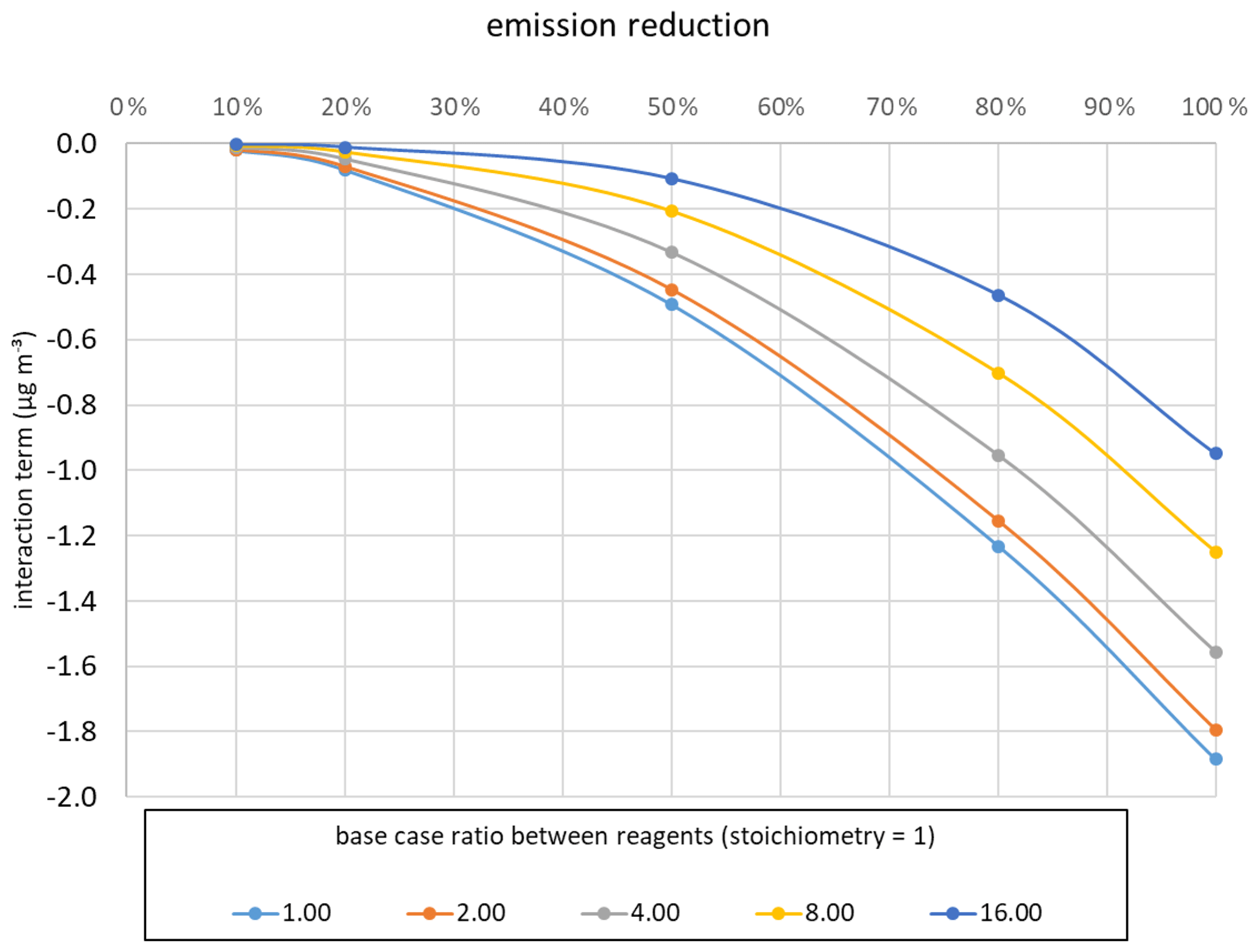
Figure A1 Variation of the interaction terms as a function of the NH₃ and HNO₃ emission reduction for different stoichiometric ratios ranging from a non-limited regime (r=1) to a strongly limited regime (r=16). Calculations were performed for conditions in which K=4 ppb².

In the base case, the concentrations of the reagents are a=[NH₃(g)] and b=[HNO₃(g)].

$$\begin{array}{ll}{\displaystyle }& {\displaystyle }\text{In case only the source of ammonia (A) is reduced,}\\ \text{(A12)}& {\displaystyle }& {\displaystyle }\mathrm{\Delta }C=\mathrm{\Delta }{C}_{\mathrm{A}}\text{with}K=(b+\mathrm{\Delta }{C}_{\mathrm{A}})(a/q+\mathrm{\Delta }{C}_{\mathrm{A}}).{\displaystyle }& {\displaystyle }\text{In case only the source of nitric acid precursors (B) is reduced,}\\ \text{(A13)}& {\displaystyle }& {\displaystyle }\mathrm{\Delta }C=\mathrm{\Delta }{C}_{\mathrm{B}}\text{with}K=(b/q+\mathrm{\Delta }{C}_{\mathrm{B}})(a+\mathrm{\Delta }{C}_{\mathrm{B}}).{\displaystyle }& {\displaystyle }\text{In case both sources are reduced,}\\ \text{(A14)}& {\displaystyle }& {\displaystyle }\mathrm{\Delta }C=\mathrm{\Delta }{C}_{\text{AB}}\text{with}K=(a/q+\mathrm{\Delta }{C}_{\text{AB}})(b/q+\mathrm{\Delta }{C}_{\text{AB}}).\end{array}$$

Solving these second-order equations for different emission reductions (represented by q in Eqs. A12–A14) shows that the inequality $\mathrm{\Delta }{C}_{\text{AB}}<\mathrm{\Delta }{C}_{\mathrm{A}}+\mathrm{\Delta }{C}_{\mathrm{B}}$ (i.e. ${\widehat{c}}_{\text{AB}}<\mathrm{0}$) is always observed (Fig. A1). Moreover, the interaction terms vary in a non-linear way with respect to the emission reduction, becoming less negative when the system moves away from stoichiometric conditions (Fig. A1).

A2.5 Compensation

In addition to the determinants described in the previous sections, which are mainly associated with the modellistic approaches used to estimate source impacts and with atmospheric chemistry, there are other factors that may alter the linearity of the relationship between the emission reductions ΔE and the response ΔC. In this section, we generically refer to such alterations as compensation.

Compensations are all the processes taking place in real-world conditions which alter the ΔC expected to result from a given ΔE in a theoretical exercise (either at the single cell or at the entire grid level), leading to interaction terms different from those expected only on the basis of applied emission reduction.

Compensation of precursor emissions: the actual emission reduction (ΔE) of one precursor is lower than the expected ΔE in a system with few sources because in a complex system, like the one analysed in this study, there are other sources of the same precursor in the grid. Consequently, the reduction in its concentration (ΔC) may not be proportional to the reduction (ΔE) of one emission source.

Compensation of precursor concentrations: the actual ΔC is different from the one expected from ΔE because there is import (advection) of this precursor from neighbouring grid cells or export (advection or deposition) from the considered grid cell.

Below are presented examples of how the compensation may affect the interaction terms in different chemical regimes.

• (a)

  The compensation alters the excess of the non-limiting precursor when emissions from not-considered sources or advection from other cells contribute significantly to the concentration of this precursor and consequently prevent the applied emission reduction from triggering a non-linear response (see Sect. A2.2).

• (b)

  The compensation alters the chemical regime. This can occur in different ways.

  • (b1)

    Emissions from unconsidered sources or advection processes are such that they keep the concentration of a limiting precursor at the stoichiometric ratio, with other precursors leading to larger negative interactions terms than those expected (see Sect. A2.1).

  • (b2)

    Advection or deposition processes may reduce the level of a non-limiting precursor to levels close to the stoichiometric ratio with other precursors and consequently lead to more negative interaction terms as described in Sect. A2.1.

  • (b3)

    Compensation may also alter the concentration of a precursor which is in competition with another. For instance, when the emissions from three major sources (e.g. AGR, TRA, IND) are reduced, other sources (e.g. energy industry, residential heating) may become predominant in controlling the chemical regime of SIA formation, which may result in novel inhibition or competition situations (e.g. Sect. A2.4).