Improving dust simulations in WRF-Chem v4.1.3 coupled with the GOCART aerosol module

In this paper, we rectify inconsistencies that emerge in the Weather Research and Forecasting model with chemistry (WRF-Chem) v3.2 code when using the Goddard Chemistry Aerosol Radiation and Transport (GOCART) aerosol module. These inconsistencies have been reported, and corrections have been implemented in WRF-Chem v4.1.3. Here, we use a WRF-Chem experimental setup configured over the Middle East (ME) to estimate the effects of these inconsistencies. Firstly, we show that the old version underestimates the PM_2.5 diagnostic output by 7 % and overestimates PM₁₀ by 5 % in comparison with the corrected one. Secondly, we demonstrate that submicron dust particles' contribution was incorrectly accounted for in the calculation of optical properties. Therefore, aerosol optical depth (AOD) in the old version was 25 %–30 % less than in the corrected one. Thirdly, we show that the gravitational settling procedure, in comparison with the corrected version, caused higher dust column loadings by 4 %–6 %, PM₁₀ surface concentrations by 2 %–4 %, and mass of the gravitationally settled dust by 5 %–10 %. The cumulative effect of the found inconsistencies led to the significantly higher dust content in the atmosphere in comparison with the corrected WRF-Chem version. Our results explain why in many WRF-Chem simulations PM₁₀ concentrations were exaggerated. We present the methodology for calculating diagnostics we used to estimate the impacts of introduced code modifications. We share the developed Merra2BC interpolator, which allows processing Modern-Era Retrospective Analysis for Research and Applications, version 2 (MERRA-2) output for constructing initial and boundary conditions for chemical species and aerosols.

1 Introduction

Produced by wind erosion, mineral dust is one of the major drivers of climate over the Middle East (ME) (Osipov et al., 2015). Dust suspended in the atmosphere affects the energy budget by absorbing and scattering incoming solar radiation (Miller and Tegen, 1998) and by affecting cloud radiative properties (Forster et al., 2007). Dust can also negatively impact infrastructure and technology. For instance, reducing solar radiation reaching the Earth's surface dust decreases the output of photovoltaic systems. Moreover, dust deposition on solar panels deteriorates their efficiency (Sulaiman et al., 2014). Dust also has socioeconomic implications. Bangalath and Stenchikov (2015) showed that due to high dust loading, the tropical rain belt across the ME and north Africa strengthens and shifts northward, causing up to a 20 % increase in summer precipitation over the semi-arid strip south of the Sahara, including the Sahel. Frequent dust outbreaks have a profound effect on air quality in the ME region (Banks et al., 2017; Farahat, 2016; Alghamdi et al., 2015; Lihavainen et al., 2016). Air pollution is characterized by near-surface concentrations of particulate matter (PM), which comprise both PM_2.5 and PM₁₀ (particles with diameters less than 2.5 and 10 µm, respectively). Dust is the major contributor to PM over the ME region (Ukhov et al., 2020a). The ME is also subjected to the inflow of dust from the nearby Sahara, which is another major dust source region (Osipov et al., 2015; Kalenderski and Stenchikov, 2016). Dust deposition fertilizes ocean surface waters and the seabed (Watson et al., 2000; Zhu et al., 1997).

Thus, given the impact of dust on climate, technology, human health, and ecosystems, an accurate description of dust effects in numerical models is essential. In the first place, it requires careful description of the dust cycle: from emission at the Earth's surface, to transport in the atmosphere, and, finally, to removal by deposition.

Most of the studies mentioned above were conducted within the group of Atmospheric and Climate Modeling at King Abdullah University of Science and Technology (KAUST) using the Weather Research and Forecasting model with chemistry (WRF-Chem) (Skamarock et al., 2005; Grell et al., 2005; Powers et al., 2017). WRF-Chem is a popular open-source tool that is widely used to study atmospheric chemistry, air quality, and aerosols (Jish Prakash et al., 2015; Khan et al., 2015; Kalenderski et al., 2013; Kalenderski and Stenchikov, 2016; Parajuli et al., 2019; Anisimov et al., 2017; Osipov and Stenchikov, 2018). This model has been used extensively to study aerosols and their impact on air quality (Fast et al., 2006, 2009; Ukhov et al., 2020a, b; Parajuli et al., 2020), climate (Zhao et al., 2010, 2011; Chen et al., 2014; Fast et al., 2006) and to analyze dust outbreaks (Bian et al., 2011; Chen et al., 2014; Fountoukis et al., 2016; Ma et al., 2019; LeGrand et al., 2019; Su and Fung, 2015; Eltahan et al., 2018; Bukowski and van den Heever, 2020) in the ME and north Africa (Zhang et al., 2015; Flaounas et al., 2016; Rizza et al., 2017; Karagulian et al., 2019; Rizza et al., 2018), North America (Zhao et al., 2012), India (Dipu et al., 2013; Kumar et al., 2014), and Australia (Nguyen et al., 2019). Many aforementioned studies utilized the WRF-Chem model coupled with the Goddard Chemistry Aerosol Radiation and Transport (GOCART) aerosol module (Chin et al., 2002). The GOCART module simulates major tropospheric aerosol components, including sulfate, dust, black and organic carbon, and sea salt, and includes algorithms for dust and sea salt emissions, dry deposition, and gravitational settling. The GOCART module is one of the most popular aerosol modules used in WRF-Chem (Bian et al., 2011; Dipu et al., 2013; Kumar et al., 2014; Chen et al., 2014; Su and Fung, 2015; Zhang et al., 2015; Flaounas et al., 2016; Fountoukis et al., 2016; Rizza et al., 2017; Flaounas et al., 2017; Nabavi et al., 2017; Chen et al., 2018; Rizza et al., 2018; Ma et al., 2019; LeGrand et al., 2019; Parajuli et al., 2019; Yuan et al., 2019; Ukhov et al., 2020a; Eltahan et al., 2018; Nguyen et al., 2019; Bukowski and van den Heever, 2020).

Table 1 WRF-Chem chem_opt namelist options affected by the found inconsistencies.

However, working with the WRF-Chem/GOCART modeling system, we found a few inconsistencies in the physical parameterizations which affected its performance. Firstly, we found that the diagnostic output of PM_2.5 and PM₁₀ was miscalculated. Secondly, the contribution of submicron dust particles was incorrectly accounted for in the Mie calculations of aerosol optical properties, and thus aerosol optical depth (AOD) was underestimated in comparison with observations. Thirdly, an inconsistency in the process of gravitational settling was leading to a violation of the dust and sea salt mass balance. The complete list of the WRF-Chem chem_opt namelist options that were affected is presented in Table 1.

All of these inconsistencies have affected WRF-Chem performance since 2 April 2010, when WRF-Chem v3.2 was released. We have reported all those issues, and they have been rectified in the WRF-Chem v4.1.3 code release. In this paper, we specifically discuss these corrections and evaluate how they have affected results. We demonstrate the methodology for calculating diagnostics that we used to estimate the impact of the introduced corrections. We also share with the community the Merra2BC interpolator (Ukhov and Stenchikov, 2020), which allows constructing initial and boundary conditions (IC&BC) for chemical species and aerosols using the Modern-Era Retrospective Analysis for Research and Applications, version 2 (MERRA-2) reanalysis (Randles et al., 2017). We believe that this discussion is in line with the open-source paradigm and will help users to better handle the code, understand physical links, and evaluate the sensitivity of the results to particular physical assumptions made in the code.

The paper is organized as follows: Sect. 2 describes the WRF-Chem model setup. In Sect. 3, a description of the inconsistencies found in the WRF-Chem code and their effects on the results is presented. Conclusions are presented in Sect. 4.

2 WRF-Chem experimental setup

To quantify the effects of introduced code modifications, we use our typical model setup which we previously adopted for simulating dust emissions using the WRF-Chem model coupled with the GOCART aerosol module. The WRF-Chem simulation domain (see Fig. 1) is centered at 28^∘ N, 42^∘ E, with a 10 km × 10 km horizontal grid (450 × 450 grid nodes). The vertical grid comprises 50 vertical levels with enhanced resolution closer to the ground. The model top boundary is set at 50 hPa. We use the chem_opt=300 namelist option, which corresponds to simulation using the GOCART aerosol module without ozone chemistry.

Figure 1 Simulation domain with marked locations of the AERONET sites. The red square corresponds to the dust emission area for conducting the dust mass balance check. Shaded contours correspond to source function S (Ginoux et al., 2001).

The unified Noah land surface model (sf_surface_physics=2) and the revised MM5 Monin–Obukhov scheme (sf_sfclay_physics=1) are chosen to represent land surface processes and surface layer physics. The Yonsei University scheme is chosen for planetary boundary layer (PBL) parameterization (bl_pbl_physics=1). The WRF single-moment microphysics scheme (mp_physics=4) is used for the treatment of cloud microphysics. The new Grell scheme (cu_physics=5) is used for cumulus parameterization. The Rapid Radiative Transfer Model (RRTMG) for both shortwave (ra_sw_physics=4) and longwave (ra_lw_physics=4) radiation is used for radiative transfer calculations. Only the aerosol direct radiative effect is accounted for. More details on the physical parameterizations used can be found at http://www2.mmm.ucar.edu/wrf/users/phys_references.html (last access: 20 January 2021).

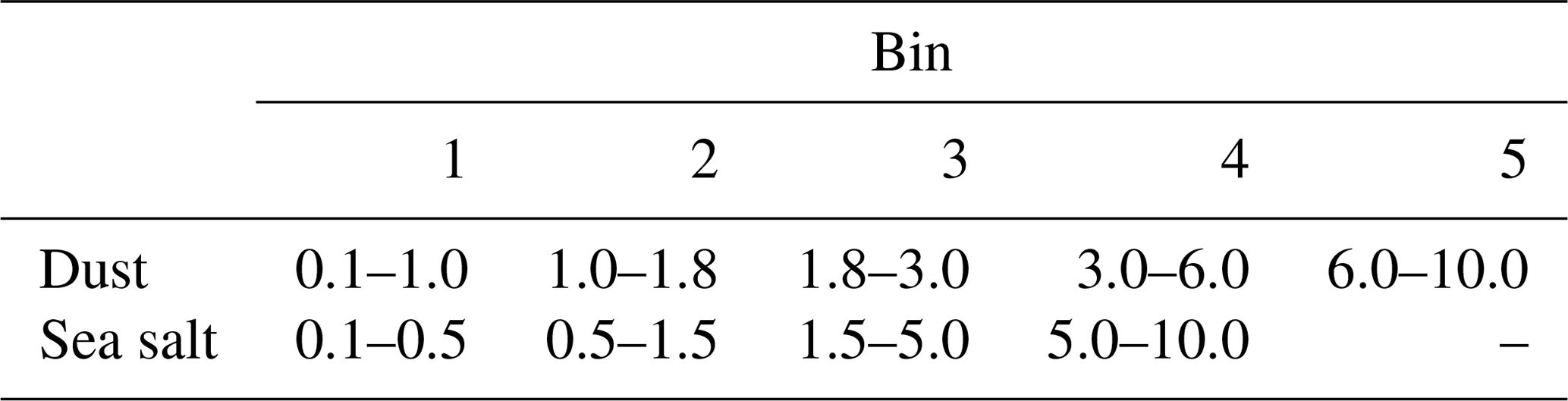
Dust size distribution in the GOCART module is approximated by five dust bins; see Table 2. Dust density is assumed to be 2500 kg m⁻³ for the first dust bin and 2650 kg m⁻³ for dust bins 2–5. In WRF-Chem, there are three dust emission schemes that can be used with GOCART: the original GOCART-WRF scheme (dust_opt=1) (Bagnold, 1941; Belly, 1964; Gillette and Passi, 1988), the Air Force Weather Agency (AFWA) scheme (dust_opt=3) (Marticorena and Bergametti, 1995; Su and Fung, 2015; Wang et al., 2015), and the University of Cologne (UoC) scheme (dust_opt=4) (Shao, 2001, 2004; Shao et al., 2011). The detailed description of all schemes is provided in LeGrand et al. (2019).

Table 2 Radii ranges (µm) of dust and sea salt bins used in the GOCART aerosol module.

Here, we simulate dust emissions using the original GOCART-WRF scheme (dust_opt=1) proposed in Ginoux et al. (2001). Dust emission mass flux, F_p (µg m⁻² s⁻¹) in each dust bin $p=\mathrm{1},\mathrm{2},\mathrm{\dots },\mathrm{5}$ is defined by the relation

$$\begin{array}{}\text{(1)}& F_p=\left\{\begin{array}{ll}CS{s}_p{u}_{\mathrm{10}\mathrm{m}}^{\mathrm{2}}\left(u_{\mathrm{10}\mathrm{m}}-u_{\mathrm{t}}\right),& \text{if }{u}_{\mathrm{10}\mathrm{m}}>u_{\mathrm{t}}\\ \mathrm{0},& \text{if }{u}_{\mathrm{10}\mathrm{m}}\le u_{\mathrm{t}},\end{array}\right.\end{array}$$

where C (µg s² m⁻⁵) is a spatially uniform factor which controls the magnitude of dust emission flux; S is the source function (Ginoux et al., 2001) (see Fig. 1) that characterizes the spatial distribution of dust emissions; u_10 m is the horizontal wind speed at 10 m; u_t is the threshold velocity, which depends on particle size and surface wetness; s_p is a fraction of dust emission mass flux within dust bin p.

Sea salt size distribution in the GOCART module is approximated by four sea salt bins (see Table 2). Sea salt density is 2200 kg m⁻³. Emission of sea salt is calculated according to Gong (2003).

2.1 Dust emission tuning

To adjust to regional conditions, dust emission in the model is calibrated to fit observed AOD and aerosol volume size distributions (AVSDs) obtained from the AErosol RObotic NETwork (AERONET; Holben et al., 1998). AERONET AOD observations represent the total AOD with contributions from all types of aerosols. But because in the ME dust is more prevalent than all other aerosols, we focus on dust emission only. More detailed information on dust emission tuning is provided in Ukhov et al. (2020a). For this study, we choose three AERONET sites (KAUST Campus, Mezaira, and Sede Boker) located within the domain (Fig. 1). We utilize level-2.0 (cloud-screened and quality-assured) AERONET AOD data. Note that from here onwards, we assume that AOD is given or calculated at 550 nm; see Appendix C.

2.1.1 Tuning the C parameter

To adjust dust emissions, we first tune the C factor from Eq. (1), as practiced in our own studies (Kalenderski et al., 2013; Jish Prakash et al., 2015; Khan et al., 2015; Kalenderski and Stenchikov, 2016; Anisimov et al., 2017; Parajuli et al., 2019, 2020; Ukhov et al., 2020a) and in the studies of other authors (Zhao et al., 2013; Kumar et al., 2014; Flaounas et al., 2017; Rizza et al., 2017). Our test runs indicate that for the ME, C=0.5 achieves a good agreement between simulated and observed AOD at the KAUST Campus, Mezaira, and Sede Boker AERONET sites. Therefore, this sub-optimal value (C=0.5) is retained in all subsequent runs.

2.1.2 Tuning the s_p fractions

We also tune s_p fractions from Eq. (1) to better reproduce the AVSDs provided by AERONET retrievals using the spectral deconvolution algorithm (SDA) (O'Neill et al., 2003). AERONET provides column-integrated AVSD dV∕dln r (µm³ µm⁻²) on 22 logarithmically equidistant discrete points in the range of radii between 0.05 and 15 µm. For AVSDs, we use the AERONET v3, level-2.0 product (Dubovik and King, 2000).

In WRF-Chem, the default values of parameter s_p from Eq. (1) are {0.1, 0.25, 0.25, 0.25, 0.25}, for the DUST₁, DUST₂, …, DUST₅ dust bins, respectively. They control the size distribution of emitted dust. Our test runs indicate that when we use the default s_p values the dust volume size distributions in the atmosphere do not match those from AERONET. To achieve a better agreement between the modeled and AERONET volume size distributions, we adjust the fractions s_p to be {0.15, 0.1, 0.25, 0.4, 0.1}. The fractions s_p are set in the phys/module_data_gocart_dust.F file, array frac_s. We effectively increase the dust emission in the finest DUST₁ and in coarse DUST₄, and decrease those in DUST₂ and DUST₅. The size distribution of emitted dust is further processed in the atmosphere.

2.2 Initial and boundary conditions for meteorological parameters, chemical species, and aerosols

As is the case with any partial differential equation solver, WRF-Chem requires the IC&BC for meteorological parameters and chemical species. IC&BC for meteorological fields are derived from the ERA-Interim (Dee et al., 2011) global atmospheric reanalysis produced by the European Centre for Medium-Range Weather Forecasts (ECMWF). IC&BC values for chemical species are required to account for initial concentrations and inflow of aerosols and chemical species. The setting of improper lateral boundary conditions for aerosols and chemistry may significantly affect the result of the simulation. The role of lateral boundary conditions increases if the domain is located close to a significant source of dust or other chemicals. Concentrations of aerosols and chemicals within the domain are especially affected by the inflow through the lateral boundaries of species with long atmospheric lifetimes.

By default, WRF-Chem uses the idealized vertical profiles of a limited number of chemical species for calculating IC&BC. These profiles are obtained from the NOAA Aeronomy Lab Regional Oxidant Model (NALROM) model (Liu et al., 1996) simulation and are representative of the northern hemispheric midlatitude (North America) summer and clean environmental conditions. Another option in WRF-Chem is to use the output from the Model for Ozone And Related chemical Tracers, version 4 (MOZART-4) (Emmons et al., 2010), which is an offline tropospheric global chemical transport model.

The MERRA-2 reanalysis (Randles et al., 2017) provides a consistent distribution of aerosols and chemical species constrained by observations with the spatial resolution about 50 km. MERRA-2 aerosol and chemical fields are superior compared to those used previously in WRF-Chem. To calculate the chemical IC&BC using MERRA-2 output, we develop an interpolator (Merra2BC; Ukhov and Stenchikov, 2020), which uses gaseous and aerosol fields from MERRA-2 reanalysis to construct the IC&BC required by the WRF-Chem simulation. For more details regarding the Merra2BC interpolator, see Appendix A.

3 Results

In the discussion below, we refer to the WRF-Chem run with all inconsistencies fixed and with properly adjusted dust emission (see Sect. 2.1), with IC&BC constructed using the developed Merra2BC interpolator (see Sect. 2.2) as ALL_OK.

To quantify the effect of each inconsistency, we perform a WRF-Chem run where all the other corrections we discuss here are implemented, with the exception that we focus on a given time. The relative difference (%) of a specific set of variables in this run with respect to the ALL_OK run is presented as a measure of sensitivity to the chosen correction. All WRF-Chem runs are performed for 1–12 August 2016. At the end of this section, we estimate the cumulative effect of all inconsistencies. For this purpose, we performed WRF-Chem simulation over the period from 1 June to 31 December of 2016.

3.1 Calculation of PM_2.5 and PM₁₀

The subroutine sum_pm_gocart in module_gocart_aerosols.F calculates PM_2.5 and PM₁₀ surface concentrations using the following formulas:

$$\begin{array}{}\text{(2)}& \begin{array}{rl}{\mathrm{PM}}_{\mathrm{2.5}}& =\mathit{\rho }\cdot \left({\mathrm{DUST}}_{\mathrm{1}}+{\mathrm{DUST}}_{\mathrm{2}}\cdot d\mathit{\_}\mathrm{25}+{\mathrm{SEAS}}_{\mathrm{1}}\right.\\ & \left.+{\mathrm{SEAS}}_{\mathrm{2}}\cdot s\mathit{\_}\mathrm{25}\right),\\ {\mathrm{PM}}_{\mathrm{10}}& =\mathit{\rho }\cdot \left({\mathrm{DUST}}_{\mathrm{1}}+{\mathrm{DUST}}_{\mathrm{2}}+{\mathrm{DUST}}_{\mathrm{3}}\right.\\ & \left.+{\mathrm{DUST}}_{\mathrm{4}}\cdot d\mathit{\_}\mathrm{10}+{\mathrm{SEAS}}_{\mathrm{1}}+{\mathrm{SEAS}}_{\mathrm{2}}+{\mathrm{SEAS}}_{\mathrm{3}}\right),\end{array}\end{array}$$

where ρ is the dry air density (kg m⁻³), DUST${}_{\mathrm{1},\mathrm{2},\mathrm{3},\mathrm{4}}$ and ${\mathrm{SEAS}}_{\mathrm{1},\mathrm{2},\mathrm{3}}$ are the mixing ratios (µg kg⁻¹) of the dust in the first four bins and sea salt in the first three bins, respectively. The contribution of the dust and sea salt bins to PM_2.5 and PM₁₀ is defined by the mapping coefficients d_25, d_10 for dust and s_25 for sea salt; see Eq. (2). Black and organic carbon and sulfate also contribute to PM, but over the ME region their contributions are small in comparison to dust and sea salt, and we omit them for the sake of brevity.

We suspect that the default mapping coefficients are calculated incorrectly. Therefore, we recalculated them assuming that dust and sea salt volume size distributions are functions of natural logarithm of particle radius. For example, interpolation in the logarithm space is more accurate than in the radius space, as aerosol size distributions are smoother functions of logarithm than radius. The updated values of mapping coefficients s_25, d_25, and d_10 along with their default values are presented in Table 3. Effectively, the contributions in PM_2.5 of sea salt SEAS₂ decreases, while that of dust DUST₂ increases. The contribution of DUST₂ in PM₁₀ decreases.

Table 3 Default and updated values of the s_25, d_25, and d_10 mapping coefficients used to calculate PM_2.5 and PM₁₀.

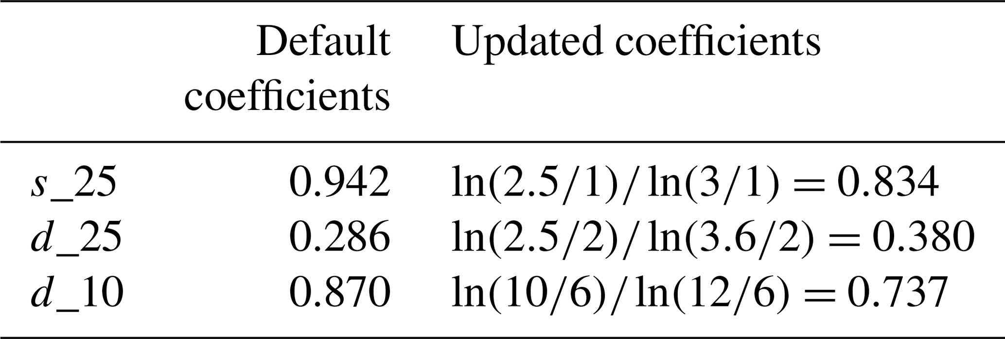
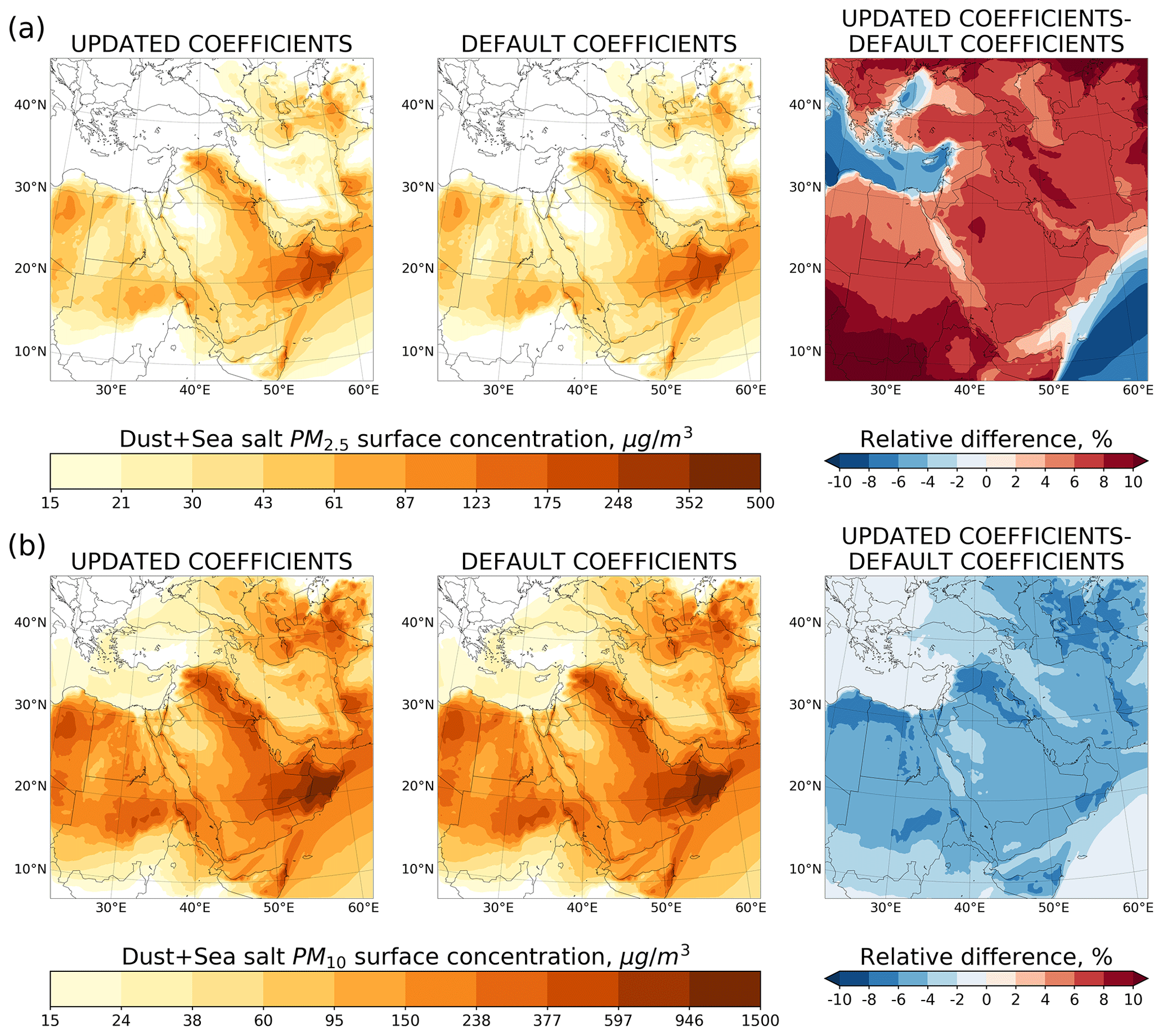
Figure 2 Average dust and sea salt PM_2.5 (a) and PM₁₀ (b) surface concentration (µg m⁻³) calculated using default and updated coefficient values and relative difference (%).

The effects of using the updated mapping coefficients in place of default ones in PM calculation are shown in Fig. 2. We calculate the PM_2.5 and PM₁₀ concentrations in the lowest model layer using Eq. (2). Surface concentrations of dust and sea salt are computed using the procedure presented in Appendix E. With the default mapping coefficients, the model on average yields 7 % lower PM_2.5 and 5 % higher PM₁₀ concentrations over the ME.

3.2 Calculation of aerosol optical properties

For modeling in the ME, the treatment of optically active dust within the model is vitally important. AOD is calculated based on aerosol number density and aerosol optical properties, which depend on the aerosol size and refractive index. In WRF-Chem, a parameterized Mie theory (Ghan and Zaveri, 2007) is employed to calculate the aerosol optical properties. This parameterization is modified for the sectional representation of the aerosol size distribution by Fast et al. (2006) and Barnard et al. (2010), so the Mie subroutine requires input of dust number density or concentration in eight size intervals: {0.039–0.078, 0.078–0.156, 0.156–0.312, 0.312–0.625, 0.625–1.25, 1.25–2.5, 2.5–5.0, and 5.0–10.0} µm. These size intervals are identical to those used in the Model for Simulating Aerosol Interactions and Chemistry (MOSAIC) microphysical module (Zaveri et al., 2008). Therefore, we further refer to them as MOSAIC bins (MOS${}_{\mathrm{1},\mathrm{2},\mathrm{3},\mathrm{4},\mathrm{5},\mathrm{6},\mathrm{7},\mathrm{8}}$).

To correctly calculate the dust optical properties, we implement two corrections in the subroutine optical_prep_gocart() in module_optical_averaging.F that compute the volume-averaged refractive index needed for Mie calculations.

3.2.1 Effect of small particles

In WRF-Chem's GOCART aerosol module, dust particle sizes span 2 orders of magnitude, from 0.1 to 10 µm; see Table 2. However, we find that dust particles with radii between 0.1 and 0.46 µm are incorrectly accounted for in the Mie calculations of aerosol optical properties. Their mixing ratio is mapped on coarser MOSAIC bins than is required. Since finer particles have a stronger effect on AOD per unit mass in comparison to coarser particles, the model AOD decreases. As a result, when tuning dust emission, we push the model to emit more dust into the atmosphere, in order to fit the observed AOD. We rectify this error by correcting mapping fractions of DUST₁ into MOSAIC bins; see Table 4.

Table 4 Dust mass redistribution between GOCART and MOSAIC bins before and after inclusion of dust particles with radii ≥ 0.1 µm into calculation of aerosol optical properties.

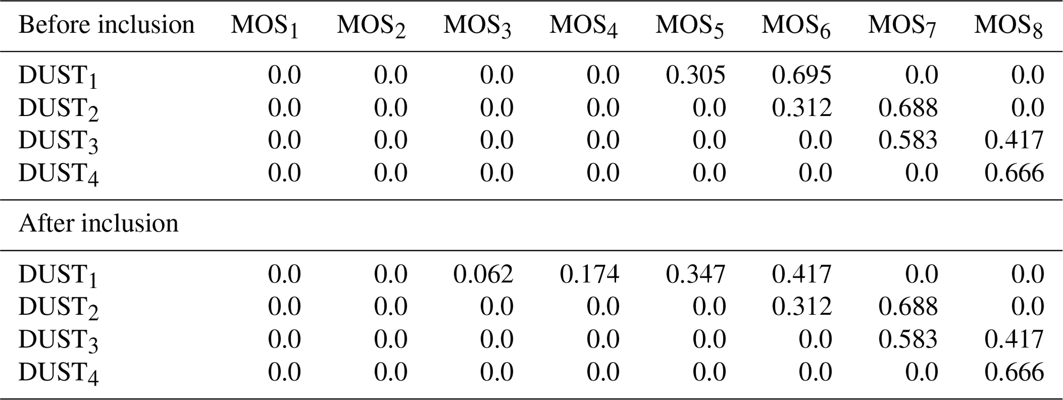
Table 4 presents the mapping fractions of the GOCART dust bins (DUST${}_{\mathrm{1},\mathrm{2},\mathrm{3},\mathrm{4}}$) to the MOSAIC bins (MOS${}_{\mathrm{1},\mathrm{2},\mathrm{3},\mathrm{4},\mathrm{5},\mathrm{6},\mathrm{7},\mathrm{8}}$) before and after correction. We do not include GOCART dust bin DUST₅ in Table 4 since it is out of the MOSAIC size range and is therefore not accounted for in the mass redistribution. Also, the mass from DUST₄ is only partially accounted for. After the changes, the dust mass from the DUST₁ bin is redistributed between finer MOS${}_{\mathrm{3},\mathrm{4},\mathrm{5},\mathrm{6}}$ bins compared to the original WRF-Chem where the entire DUST₁ mixing ratio was mapped on the coarser MOS_5,6 bins.

3.2.2 Bin concentration interpolation

Originally, the subroutine optical_prep_gocart() redistributes dust and sea salt mass from GOCART into MOSAIC bins, using the assumption that dust size distribution is a function of particle radius. Consistent with Sect. 3.1, here we conduct interpolation assuming that dust distribution is a function of natural logarithm of radius. This modification causes changes in the mass redistribution between the GOCART and MOSAIC bins (see Table 5) and increases the contribution of small dust particles into the AOD. Because the dust size distribution is a smoother function of the logarithm of a radius than the radius itself, interpolation is more accurate in logarithms than in radii.

Table 5 Dust mass redistribution between GOCART and MOSAIC bins based on the assumption that bin concentration is a function of radius and on the assumption that bin concentration is a function of natural logarithm radius.

Figure 3 AOD time series (a–c) and scatter plots (d–f) from NON_LOG_046 and ALL_OK runs (blue and red lines) and AERONET AOD (green markers) at KAUST Campus, Mezaira, and Sede Boker. WRF-Chem's AOD is interpolated to the times (blue diamonds and red dots) when AERONET AOD measurements were conducted.

To estimate the effect of these two corrections, we develop the WRF-Chem simulation NON_LOG_046, where only these two inconsistencies are not fixed, and compare the resulting AOD with that from the ALL_OK run. The AOD values are computed as described in Appendix C. As expected, the AOD increases after the corrections. Figure 3 compares the AOD obtained from the ALL_OK and NON_LOG_046 runs with AERONET AOD at KAUST Campus, Mezaira, and Sede Boker. Because AERONET conducts measurements during daylight hours only, we interpolate WRF-Chem AOD to the AERONET measurement times.

To quantify the capability of WRF-Chem in reproducing the AERONET AOD, we calculate the Pearson correlation coefficient R and mean bias (see Appendix B) of simulated AOD with respect to the AERONET AOD observations for the entire simulation period (see Table 6). The corrections improve the correlation for Mezaira and Sede Boker and cause a 2-fold reduction in the mean bias in KAUST Campus and Mezaira. The magnitude and temporal evolution of the AOD time series is well correlated in both runs (with and without corrections) with the observed AERONET AOD at all sites only when the AERONET AOD < 1. For dusty conditions with AOD > 1, WRF-Chem with the original GOCART scheme (dust_opt=1) struggles to capture the observations. We find the worst correlation (R=0.42) and highest mean bias (−0.19) with AERONET AOD at the Mezaira station, which is located in a major dust source region (see Fig. 1). We obtain higher correlations with AERONET AOD of 0.66 and 0.75 for the KAUST Campus and Sede Boker stations, respectively. Both of these stations are located outside the main dust source regions.

Table 6 Pearson correlation coefficient R and mean bias calculated for AOD time series from two runs with respect to AERONET AOD observations.

Figure 4 Averaged AOD fields obtained from the ALL_OK and NON_LOG_046 runs and their relative difference (%).

Figure 4 shows the averaged AOD fields obtained from the ALL_OK and NON_LOG_046 runs, as well as their relative difference (%). We conclude that due to these two inconsistencies, averaged AOD obtained from the NON_LOG_046 run is lower by 25 %–30 % on average over the ME in comparison with the ALL_OK run. Over Libya, Egypt, Oman, Iran, Azerbaijan, Turkmenistan, and Pakistan, the difference is even higher, reaching 30 %–35 %.

3.3 Gravitational settling

We find that in the original WRF-Chem code the gravitational settling of dust and sea salt is calculated incorrectly. The default finite-difference scheme (implemented in the subroutine settling() file module_gocart_settling.F) does not account for change in air density when it calculates deposition mass flux. Thus, in the course of the gravitational settling, the total mass of dust and sea salt in the atmosphere increases, violating their mass balances. We introduce the new finite-difference scheme, which allows conservation of the mass of dust and sea salt in the course of gravitational settling in the atmosphere. The new finite-difference scheme is provided below.

The change of aerosol mixing ratio due to gravitational settling at downward directed velocity w is given by the following differential equation:

$$\begin{array}{}\text{(3)}& {\displaystyle \frac{\partial \left(\mathit{\rho }q\right)}{\partial t}}={\displaystyle \frac{\partial \left(\mathit{\rho }qw\right)}{\partial z}},\end{array}$$

where q is the aerosol mass mixing ratio (µg kg⁻¹) and ρ is the dry air density (kg m⁻³). Using the first-order upwind scheme, this equation can be discretized into the following form:

$$\begin{array}{}\text{(4)}& {\displaystyle \frac{q_k^{n+\mathrm{1}}{\mathit{\rho }}_k^{n+\mathrm{1}}-q_k^n{\mathit{\rho }}_k^n}{\mathrm{\Delta }t}}={\displaystyle \frac{q_{k+\mathrm{1}}^n{\mathit{\rho }}_{k+\mathrm{1}}^{n+\mathrm{1}}{w}_{k+\mathrm{1}}^n-q_k^n{\mathit{\rho }}_k^{n+\mathrm{1}}{w}_k^n}{\mathrm{\Delta }{z}_k}},\end{array}$$

where Δz_k is the depth of the k model level, and Δt is the model time step. Subscript k denotes the model levels and superscript n is the time level. Taking into account that the calculation of gravitational settling is split from the calculation of the continuity equation, we assume ${\mathit{\rho }}_k^{n+\mathrm{1}}\approx {\mathit{\rho }}_k^n$ and get the following solution:

$$\begin{array}{}\text{(5)}& q_k^{n+\mathrm{1}}=q_k^n\left(\mathrm{1}-{\displaystyle \frac{\mathrm{\Delta }t{w}_k^n}{\mathrm{\Delta }{z}_k}}\right)+q_{k+\mathrm{1}}^n{\displaystyle \frac{\mathrm{\Delta }t{w}_{k+\mathrm{1}}^n}{\mathrm{\Delta }{z}_k}}{\displaystyle \frac{{\mathit{\rho }}_{k+\mathrm{1}}^{n+\mathrm{1}}}{{\mathit{\rho }}_k^{n+\mathrm{1}}}}.\end{array}$$

Equation (5) is solved for each model column from the top to the bottom.

To validate the modified finite-difference scheme, we zero dust emissions across the whole domain, except for the 200 km × 200 km area located at the center of the domain; see Fig. 1. Only the first 10 simulation hours of dust emissions within this area are included. We prohibit the inflow of dust from the domain boundaries by zeroing the corresponding boundary conditions, and we zero the initial dust concentrations to simplify calculation of the dust mass balance, which we compute using the following balance relation:

$$\begin{array}{}\text{(6)}& \begin{array}{rl}& \text{Dust in the atmosphere}=\text{Emitted dust}\\ & -(\text{Grav. settled dust}+\text{Dry deposited dust}).\end{array}\end{array}$$

The amount of dust in the atmosphere is controlled by dust emission and dust deposition. The latter comprises gravitational settling and dry deposition. For the sake of clarity, we refrain from introducing other dust removal processes, such as subgrid wet deposition (conv_tr_wetscav=0). The procedure of calculation of these diagnostics using the WRF-Chem output is provided in Appendix F.

Figure 5 Dust mass balance check (a) before and (b) after correction of gravitational settling. Deposited dust is the combination of gravitationally settled dust and dry deposited dust.

Figure 5 demonstrates the evolution of the components of the dust mass balance (see Eq. 6) from the two runs, with and without correction of the gravitational settling procedure. For the analysis, we took only the first 40 h of output because, after that time the dust plume reaches the lateral boundaries of the domain. As shown in Fig. 5a, the dashed red line corresponding to the sum of deposited mass and dust mass in the atmosphere diverges from the dash-dotted purple line, which corresponds to the mass of emitted dust. This difference reaches 2.16 % before the dust plume reaches the boundaries of the domain. The run using the original gravitational settling gains the dust mass represented by the blue line, due to the error in calculating gravitational settling, as discussed above. This is in contrast with Fig. 5b, where we see perfect agreement between the amounts of deposited dust plus dust in the atmosphere and emitted dust until the dust plume reaches the boundaries of the domain. Thus, this inconsistency in the gravitational settling subroutine is significant, as the error of 2.16 % of total emitted mass accumulates within ≈ 20 h. For a larger domain, this imbalance will be more significant. This effect is especially important in the low-latitude desert regions. Zhang et al. (2015), Dipu et al. (2013), and Huang et al. (2010) reported that in dry subtropics the boundary layer height can reach 6–7 km, which promotes the transport of dust particles to this altitude. When dust particles are settling from higher altitudes, a larger mass imbalance is accumulated.

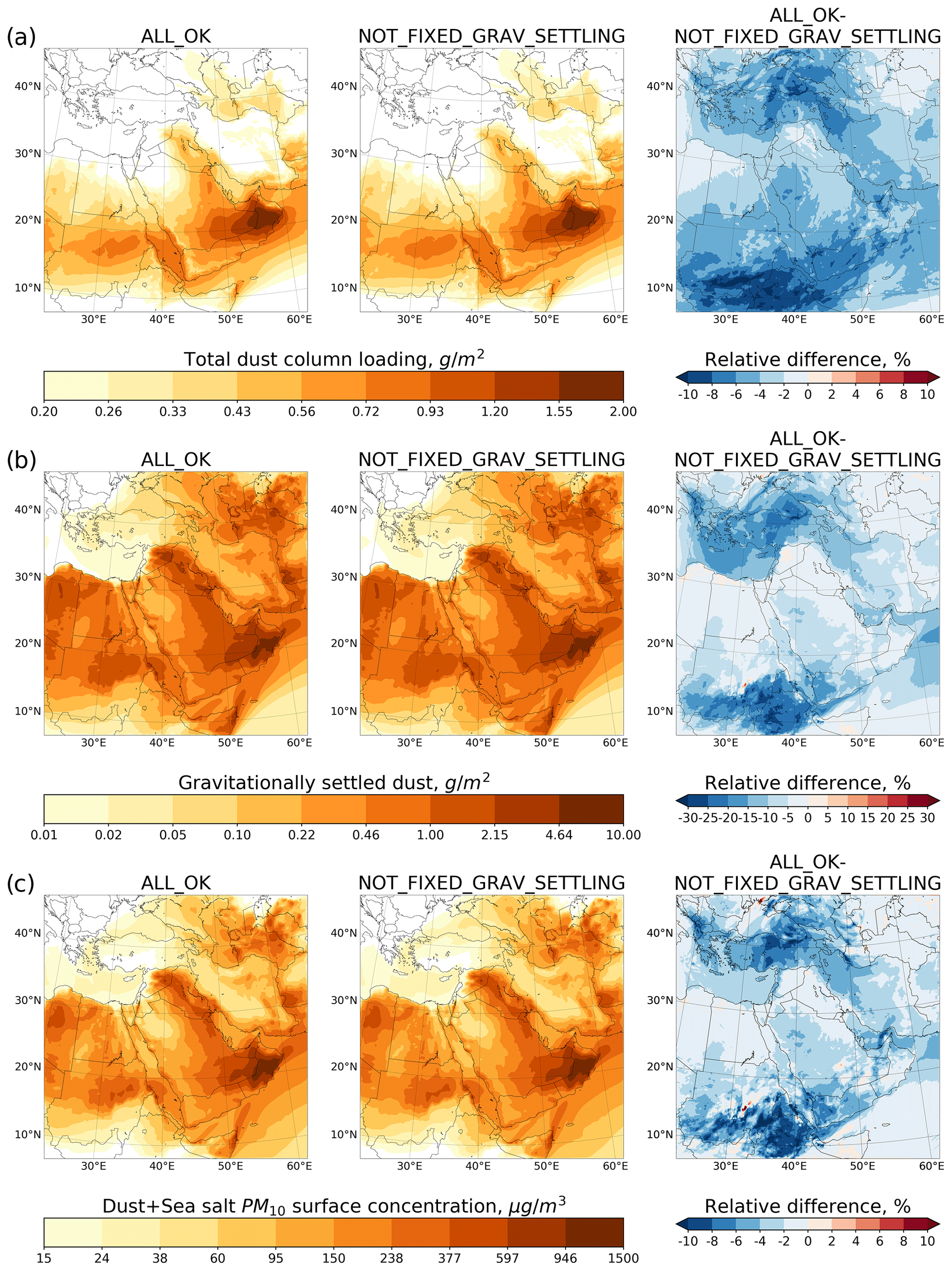
Figure 6 Comparison of ALL_OK and NOT_FIXED_GRAV_SETTLING runs. (a) Averaged total dust column loadings (g m⁻²) and relative difference (%). (b) Gravitationally settled dust (g m⁻²) and relative difference (%). (c) Averaged dust and sea salt PM₁₀ surface concentrations (µg m⁻³) and relative difference (%).

We estimate the effect of the gravitational settling error by comparing averaged total dust column loadings (see Fig. 6a), accumulated gravitationally settled dust (see Fig. 6b), and averaged dust and sea salt PM₁₀ surface concentrations (see Fig. 6c) obtained in the ALL_OK and NOT_FIXED_GRAV_SETTLING runs, where the latter corresponds to the run with error in gravitational settling. We perform a comparison in terms of relative differences (%) in the runs, with and without corrections. Dust column loadings, gravitationally settled dust, and PM₁₀ surface concentrations are calculated according to the methodology described in Appendix Sects. D, F3, and E, respectively. According to Fig. 6a–c, we observe higher negative values of relative difference over non-dust-source regions (see Fig. 1), i.e., over Sudan, Turkey, Yemen, Eritrea, Djibouti, and Ethiopia. In contrast, the relative differences over dust source regions, which include Egypt and the eastern part of Arabian Peninsula, are close to zero. Coarse dust particles have shorter lifetimes in the atmosphere because of their higher deposition velocities. Thus, coarse dust particles are mostly deposited in the dust source regions, which explains close to zero values of relative difference in this region. Fine dust particles have longer atmospheric lifetime and thus can be transported over longer distances. The discrepancies in the descriptions of the life cycle of fine dust explain larger relative errors in non-dust regions, as mentioned above.

Thus, we can conclude that in the NOT_FIXED_GRAV_SETTLING run, the total dust column loading is higher by 4 %–6 % over the ME in comparison with the ALL_OK run. The computed total amount of dust in the atmosphere (see Appendix F4) was 6.41 and 6.72 Tg for the ALL_OK and NOT_FIXED_GRAV_SETTLING runs, respectively. Hence, the amount of dust in the atmosphere is around 4.8 % higher. The total amount of gravitationally settled dust is 5 %–10 % higher on average in NOT_FIXED_GRAV_SETTLING run. The biggest difference (15 %–25 %) is observed in Sudan, Yemen, Eritrea, Djibouti, Ethiopia, and Turkey. The computed total amount of gravitationally settled dust (see Appendix F3) was 11 and 11.55 Tg for ALL_OK and NOT_FIXED_GRAV_SETTLING runs, respectively. Hence, the amount of gravitationally settled dust is around 5 % higher in the NOT_FIXED_GRAV_SETTLING run. Dust and sea salt PM₁₀ surface concentrations (see Eq. 2 and Appendix E) are higher by 2 %–4 % on average over the ME in comparison with the ALL_OK run. We observe even bigger differences (6 %–10 %) over Eritrea, Djibouti, Ethiopia, and Turkey.

3.4 Case study

In the previous sections, we separately quantified the effect of each inconsistency in the WRF-Chem code and explained the associated physical links using short-term runs. In this section, we conduct a 7-month case study to demonstrate the cumulative effect of all inconsistencies. We ran two WRF-Chem simulations from 1 June to 31 December 2016, using the experimental setup described in Sect. 2. We refer to the WRF-Chem run, where all inconsistencies are intact, as ALL_OLD. We compare it with ALL_OK run in which all inconsistencies are corrected. The simulation period is chosen to take advantage of PM₁₀ surface concentrations measurements conducted by the Saudi Authority for Industrial Cities and Technology Zones (MODON) in Riyadh, Jeddah, and Dammam (megacities of Saudi Arabia). More details on these measurements are provided in Ukhov et al. (2020a).

Figure 7 Daily averaged AOD time series from the ALL_OK and ALL_OLD runs (red and blue lines) and AERONET AOD (green line) at KAUST Campus, Mezaira, and Sede Boker.

To adjust dust emissions in ALL_OLD run, we tuned the C factor from Eq. (1). Our test runs indicated that C=0.8 provides the best agreement between simulated and observed AOD. For the ALL_OK run, we used C=0.5 as before. Comparison of daily averaged AOD time series obtained from the ALL_OK and ALL_OLD runs with the AERONET AODs at KAUST Campus, Mezaira, and Sede Boker is presented in Fig. 7. AODs from both experiments are in good agreement with the AERONET AOD. The Pearson correlation coefficients and mean biases (see Appendix B) with respect to AERONET AOD are in the ranges of 0.62–0.75 and −0.03–0.07, respectively, for all AERONET sites. Thus, in the ALL_OLD run, the incorrect mapping of dust particles with radii between 0.1 and 0.46 µm causes stronger dust emissions in comparison with ALL_OK run.

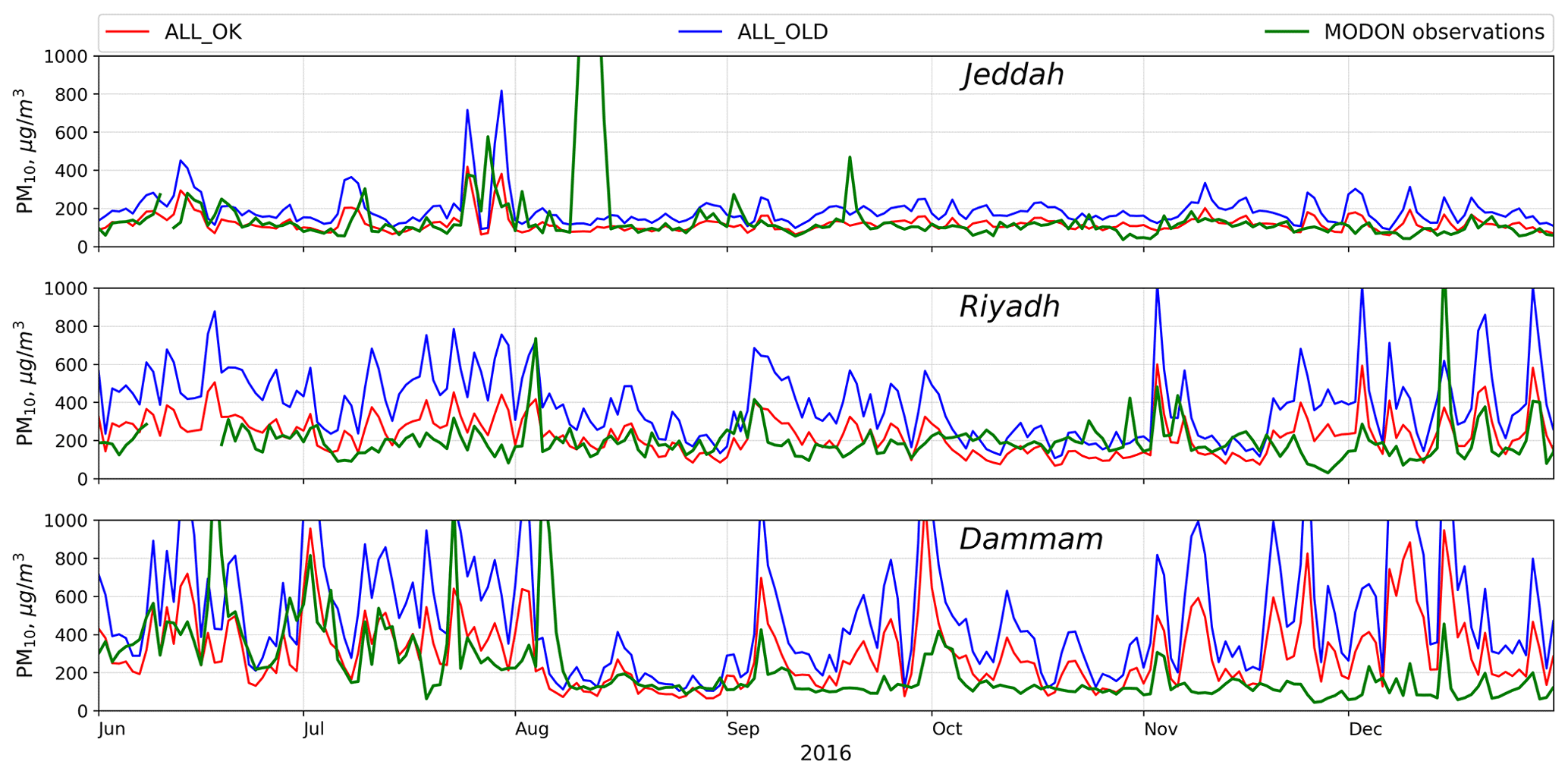
Figure 8 Daily averaged PM₁₀ surface concentrations (µg m⁻³) from the ALL_OK and ALL_OLD runs (red and blue lines) and from MODON observations (green line) at Jeddah, Riyadh, and Dammam.

The stronger dust emissions lead to increased dust surface concentrations and increased dust content in the atmosphere. Figure 8 shows comparison of the daily averaged PM₁₀ surface concentrations obtained from the ALL_OK and ALL_OLD runs and from MODON observations in Riyadh, Jeddah, and Dammam. Modeled PM₁₀ concentrations were computed using Eq. (2). PM₁₀ constituents were sampled at the exact MODON stations locations. We used “default” and “updated” mapping coefficients (s_25, d_25, and d_10; see Table 3) for the evaluation of PM₁₀ concentrations from the ALL_OLD and ALL_OK runs, respectively. Average MODON PM₁₀ concentrations are 136, 206, and 229 (µg m⁻³) for Jeddah, Riyadh, and Dammam, respectively. PM₁₀ concentration time series from the ALL_OK run demonstrate better agreement with the MODON observations in comparison with the PM₁₀ time series from the ALL_OLD run. In particular, mean biases with respect to MODON observations for ALL_OK and ALL_OLD runs are 2, 23, and 77, and 72, 182, and 275 (µg m⁻³) for Jeddah, Riyadh, and Dammam, respectively; see Fig. 8. Thus, the PM₁₀ concentration bias in ALL_OK is lower by 50 %–85 % in comparison with the ALL_OLD run.

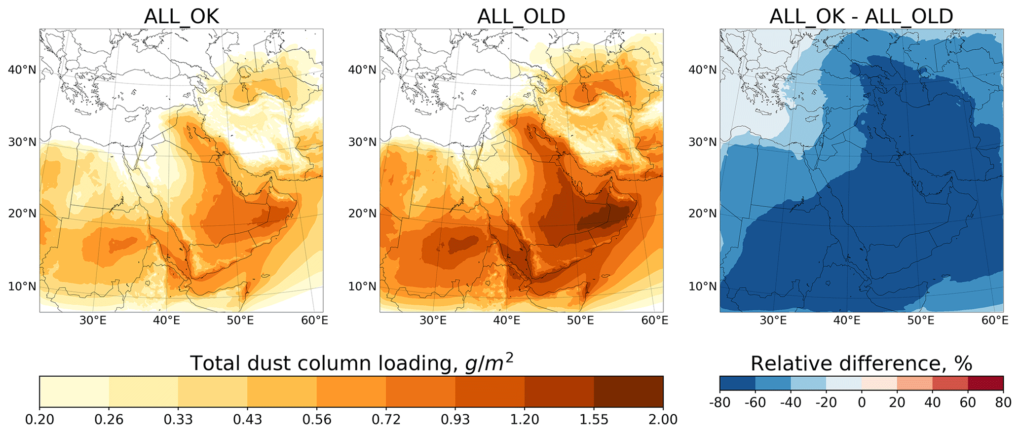
Figure 9 Averaged over the summer (June, July, August) of 2016 total dust column loadings (g m⁻²) from the ALL_OK and ALL_OLD runs and relative difference (%).

Figure 9 demonstrates the averaged over the summer (June, July, August) of 2016 total dust column loadings (g m⁻²) and their relative differences (%) obtained from the ALL_OK and ALL_OLD runs. In some locations, dust content in the atmosphere from the ALL_OLD run is higher by 80 % in comparison with the ALL_OK run. The total mass of dust in the atmosphere in the ALL_OK run yields 6.68 Tg in comparison with 10.92 Tg in the ALL_OLD run, so the difference exceeds 60 %.

3.5 Effect of initial and boundary conditions

We specifically conduct a sensitivity simulation to examine the impact of boundary conditions on PM₁₀ surface concentration over the ME. In this simulation, boundary conditions are constructed using the developed Merra2BC interpolator (Ukhov and Stenchikov, 2020) (see Appendix A), and we zero the initial concentrations of dust and sea salt. The emissions of dust and sea salt within the domain are turned off (dust_opt=0, seas_opt=0). In this instance, PM₁₀ concentrations are entirely determined by the inflow from the lateral boundaries. The averaged PM₁₀ surface concentrations are presented in Fig. 10. PM₁₀ concentrations are calculated using Eq. (2). Figure 10 shows the inflow of PM₁₀ from Africa, central Asia, and the Indian Ocean. Dust is the major contributor to the PM₁₀ transported from Africa and central Asia, whereas sea salt contributes to PM₁₀ transported over the Indian Ocean.

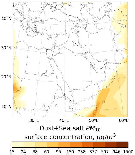
Figure 10 Effect of transboundary transport. Averaged dust and sea salt PM₁₀ surface concentrations (µg m⁻³) are obtained from the WRF-Chem simulation without emission of sea salt and dust.

4 Conclusions

In this paper, we discuss the inconsistencies found in the WRF-Chem v3.2 model coupled with the GOCART aerosol module. All of these inconsistencies are rectified in the WRF-Chem v4.1.3 code release. Here, we demonstrate the effect of the code rectification on WRF-Chem model performance. We also demonstrate the methodology we employ to calculate diagnostics, which we then use to estimate the effects of the changes made. To make these assessments, we configure the WRF-Chem domain over the ME and run it with 10 km grid resolution. The runs discussed in this paper were performed over the period of 1–12 August 2016. The effect of each inconsistency was estimated using specifically designed WRF-Chem runs where only one model inconsistency was activated.

We found that in WRF-Chem v3.2 coupled with GOCART, the inconsistency in diagnostics of PM surface concentration caused a 7 % decrease in PM_2.5 and a 5 % increase in PM₁₀ surface concentrations. Due to drawback in mapping of dust particles with radii between 0.1 and 0.46 µm from GOCART to MOSAIC bins for Mie calculations of aerosol optical properties, the modeled AOD was decreased by 25 %–30 % in comparison with the corrected WRF-Chem version. This led to higher dust emissions and surface PM concentrations, because the WRF-Chem model is tuned to fit the simulated AOD to AERONET observations. This explains the inconsistencies found in Kumar et al. (2014), Eltahan et al. (2018), and Flaounas et al. (2017). Flaounas et al. (2017) noted that the model simulates realistic AODs when dust emissions are exaggerated, which in turn results in exaggerated dust surface concentrations. Conversely, realistic reproduction of dust concentration yields AODs that are smaller than in observations. Because of the error in calculating gravitational settling, dust column loadings increased by 4 %–6 % and the mass of gravitationally settled dust increased by 5 %–10 % in comparison with the corrected WRF-Chem version. The contribution of dust and sea salt into PM₁₀ surface concentration was also higher by 2 %–4 % on average over the ME.

The cumulative effect of all inconsistencies was estimated in the 7-month case study conducted for 1 June–31 December 2016, when both AERONET AODs and PM₁₀ surface observations were available. The comparison of runs with and without proposed changes shows that the run without corrections yields higher dust loadings and total dust mass in the atmosphere by 80 % and 60 %, respectively. This 7-month case study shows that the cumulative response to all code modifications applied simultaneously is stronger than the sum of their partial contributions. For instance, AOD underestimation causes higher dust emissions, which causes higher dust surface concentrations and increased production of dust in the atmosphere due to the error in gravitational settling. As a consequence, PM₁₀ surface concentration further increases. Finally, an already high PM₁₀ surface concentration becomes even higher due to the incorrect calculation of PM₁₀. Thus, the proposed improvements help to explain the considerable bias towards higher PM₁₀ concentrations found in Ma et al. (2019), Flaounas et al. (2017), Su and Fung (2015), Nabavi et al. (2017), Rizza et al. (2017), and Eltahan et al. (2018).

In the course of improving the simulation of natural and anthropogenic aerosols and chemicals, we developed the capability to use MERRA-2 reanalysis for constructing WRF-Chem initial and boundary conditions for chemical species and aerosols. The interpolation utility Merra2BC was coded for this purpose. Boundary conditions constructed using MERRA-2 reanalysis more realistically account for the transboundary transport of aerosols. Merra2BC is made available to the community.

We believe the detailed quantification of the effects of the recent WRF-Chem code improvements are in line with open-source principles. The results of this work aim at better understanding of the model sensitivities to physical parameterizations. This work will add a greater understanding of model performance and will be especially helpful for those who use the WRF-Chem model coupled with the GOCART aerosol module to carry out dust simulations over regions where dust plays an important role.

Appendix A: Merra2BC interpolator

The Merra2BC interpolator (Ukhov and Stenchikov, 2020) (available online at https://github.com/saneku/Merra2BC) creates initial and boundary conditions based on MERRA-2 reanalysis (Randles et al., 2017) for a WRF-Chem simulation by interpolating chemical species mixing ratios defined on the MERRA-2 grid to WRF-Chem grid. For the initial conditions, interpolated values are written to each node of the WRF-Chem grid. For the boundary conditions, only boundary nodes are affected.

Merra2BC is written in Python. The utility requires additional modules that need to be installed in the Python environment: NetCDF4 (netcdf4, https://github.com/Unidata/netcdf4-python, last access: 20 January 2021) interface to work with NetCDF files and SciPy's (scipy, https://github.com/scipy/scipy, last access: 20 January 2021) interpolation package.

The full MERRA-2 reanalysis data set including aerosol and gaseous collections is publicly available online (https://disc.gsfc.nasa.gov/daac-bin/FTPSubset2.pl, last access: 20 January 2021). Depending on the requirements, all or one of the following aerosol and gaseous collections need to be downloaded: inst3_3d_aer_Nv – gaseous and aerosol mass mixing ratios, (kg kg⁻¹) and inst3_3d_chm_Nv – carbon monoxide and ozone mass mixing ratios, (kg kg⁻¹). Besides downloaded mass mixing ratios, pressure thickness DELP and surface pressure PS fields also need to be downloaded. Spatial coverage of the MERRA-2 files should include the area of the simulation domain. The time span of the downloaded files should match the start and duration of the simulation. More information regarding MERRA-2 files' specification is provided in Bosilovich et al. (2016).

A1 Reconstruction of the pressure in MERRA-2 and in WRF-Chem

Atmospheric pressure is used as a vertical coordinate. Latitude and longitude serve as the horizontal coordinates.

The MERRA-2 vertical grid has 72 model layers which are on a terrain-following hybrid σ−p coordinate. The pressure at the model top is a fixed constant, P_TOP=0.01 hPa. Pressure at the model edges is computed by summing the DELP starting at P_TOP. A representative pressure for the layer can then be obtained by averaging pressure values on adjacent edges. Indexing for the vertical coordinate is from top to bottom; i.e., the first layer is the top layer of the atmosphere (P_TOP), while the 72nd layer is adjacent to the Earth's surface.

In WRF-Chem, the pressure field is not given in wrfinput_d01 and wrfbdy_d01 files. Hence, the pressure field must be restored using surface pressure P_SFC taken from met_em_...* files created by metgrid.exe during the preprocessing stage. Pressure at the top of the model wrf_p_top and η values on half levels (znu) are taken from the wrfinput_d01 file. The procedure of reconstructing the pressure from met_em_...* files using the Python code is demonstrated in Fig. A1.

Figure A1 A Python script, which reconstructs the pressure using the met_em_...* files. nx, ny, and nz indicate the number of grid nodes in WRF-Chem domain.

A2 Mapping chemical species between MERRA-2 and WRF-Chem

Merra2BC file config.py contains multiplication factors to convert MERRA-2 mass mixing ratios of gases given in kg kg⁻¹ into ppmv. Aerosols are converted from kg kg⁻¹ to µg kg⁻¹. When using the GOCART aerosol module in WRF-Chem simulation, all MERRA-2 aerosols and gases are matched with those from WRF-Chem. We simply multiply by a factor of 10⁹ to convert MERRA-2 aerosol mixing ratios given in kg kg⁻¹ into µg kg⁻¹. In the case of gases, we need to multiply MERRA-2 mass mixing ratios by a ratio of molar masses M_air∕M_gas multiplied by 10⁶ to convert kg kg⁻¹ into ppmv, where M_gas and M_air are molar masses (g mol⁻¹) of the required gas and air (28.97 g mol⁻¹), respectively. If another aerosol module is chosen in WRF-Chem, then different multiplication factors should be used.

A3 Interpolation procedure

A brief description of the interpolation procedure applied to the initial conditions is presented in Fig. A2.

Figure A2 Interpolation procedure applied to initial conditions.

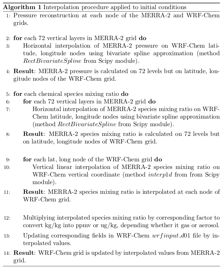
For boundary conditions, the procedure is similar, except that additional updates of domain boundary tendencies are required and interpolation is performed for each step, where boundary conditions are applied.

A4 Typical workflow

Here are the steps describing how to work with the Merra2BC interpolator:

1. Run real.exe, which will produce initial wrfinput_d01 and boundary conditions wrfbdy_d01 files required by the WRF-Chem simulation.

2. Download required MERRA-2 files from https://disc.gsfc.nasa.gov/daac-bin/FTPSubset2.pl;

3. Download Merra2BC from https://github.com/saneku/Merra2BC.

4. Edit the config.py file which contains

   • a.

     mapping of chemical species and aerosols between MERRA-2 and WRF-Chem;

   • b.

     paths to wrfinput_d01, wrfbdy_d01, and met_em_...* files;

   • c.

     a path to the downloaded MERRA-2 files.

5. real.exe sets default boundary and initial conditions for some chemical species. Merra2BC adds interpolated values to the existing values, which may cause incorrect concentration values. To avoid this, run “python zero_fileds.py”, which will zero the required fields.

6. Run “python main.py”, which will do the interpolation. As a result, files wrfinput_d01 and wrfbdy_d01 will be updated by the interpolated from MERRA-2 values.

7. Modify the WRF-Chem namelist.input file at section &chem: set have_bcs_chem = .true. to activate updated boundary conditions and, if needed, chem_in_opt = 1 to activate updated initial conditions.

8. Run wrf.exe.

Appendix B: Statistics

The following statistical parameters were used to quantify the level of agreement between estimations and observations.

For the Pearson correlation coefficient (R),

$$\begin{array}{}\text{(B1)}& R={\displaystyle \frac{\sum _{i=\mathrm{1}}^N\left(F_i-\stackrel{\mathrm{‾}}{F}\right)\left(O_i-\stackrel{\mathrm{‾}}{O}\right)}{\sqrt{\sum _{i=\mathrm{1}}^N{\left(F_i-\stackrel{\mathrm{‾}}{F}\right)}^{\mathrm{2}}\sum _{i=\mathrm{1}}^N{\left(O_i-\stackrel{\mathrm{‾}}{O}\right)}^{\mathrm{2}}}}}.\end{array}$$

For the mean bias (bias),

$$\begin{array}{}\text{(B2)}& \mathrm{bias}={\displaystyle \frac{\mathrm{1}}{N}}\sum _{i=\mathrm{1}}^N\left(F_i-O_i\right),\end{array}$$

where F_i is the estimated value, O_i is the observed value, $\stackrel{\mathrm{‾}}{F}=\frac{\mathrm{1}}{N}\sum _{i=\mathrm{1}}^N{F}_i$ and $\stackrel{\mathrm{‾}}{O}=\frac{\mathrm{1}}{N}\sum _{i=\mathrm{1}}^N{O}_i$ their averages, and N is the number of data.

Appendix C: AOD calculations

WRF-Chem does not calculate AOD at 550 nm (only at 300, 400, 600, and 1000 nm for variables TAUAER1, TAUAER2, TAUAER3, and TAUAER4, respectively), but instead it outputs the extinction coefficient at 550 nm (variable EXTCOF55). The AOD at 550 nm (AOD₅₅₀) for the (i,j) vertical column can be calculated by summing throughout the vertical column of product of multiplication of the EXTCOF55 by the Δz:

$$\begin{array}{}\text{(C1)}& {\mathrm{AOD}}_{\mathrm{550}i,j}=\sum _k\mathrm{EXTCOF}{\mathrm{55}}_{i,j,k}\cdot \mathrm{\Delta }{z}_{i,j,k},\end{array}$$

where $\mathrm{\Delta }{z}_{i,j,k}$ is the depth (m) of the ($i,j,k$) cell, which can be computed using the formula:

$$\begin{array}{}\text{(C2)}& \begin{array}{rl}\mathrm{\Delta }{z}_{i,j,k}& =\left({\mathrm{PH}}_{i,j,k}+{\mathrm{PHB}}_{i,j,k}\right)/g\\ & -\left({\mathrm{PH}}_{i,j,k-\mathrm{1}}+{\mathrm{PHB}}_{i,j,k-\mathrm{1}}\right)/g,\end{array}\end{array}$$

where PH is the geopotential and PHB is the perturbed geopotential, and g=9.81 m s² is the gravitational acceleration. Variables PH and PHB are taken from the WRF-Chem output.

To facilitate comparison with the model output, the 550 nm AOD is calculated using the following relation:

$$\begin{array}{}\text{(C3)}& {\displaystyle \frac{{\mathit{\tau }}_{\mathit{\lambda }}}{{\mathit{\tau }}_{{\mathit{\lambda }}_{\mathrm{0}}}}}={\left({\displaystyle \frac{\mathit{\lambda }}{{\mathit{\lambda }}_{\mathrm{0}}}}\right)}^{-\mathit{\alpha }},\end{array}$$

where α is the Ångström exponent for the 440–675 nm wavelength range provided by AERONET, τ_λ is the optical thickness at wavelength λ, and ${\mathit{\tau }}_{{\mathit{\lambda }}_{\mathrm{0}}}$ is the optical thickness at the reference wavelength λ₀.

Appendix D: Column loadings

WRF-Chem stores dust column loadings (µg m⁻²) using variables DUSTLOAD_1,2,3,4,5. Column loadings for the (i,j) vertical column of other aerosols or chemical species can be computed by vertically summing throughout the vertical column of product of multiplication of the mass mixing ratio q (µg kg⁻¹) by the cell depth Δz (m) (see Eq. C2) and dry air density (kg m⁻³). WRF outputs variable ALT, which is inverse dry air density (m³ kg⁻¹):

$$\begin{array}{}\text{(D1)}& {\text{Column loading}}_{i,j}=\sum _k{q}_{i,j,k}\cdot \mathrm{\Delta }{z}_{i,j,k}\cdot \mathrm{1}/{\text{ALT}}_{i,j,k}.\end{array}$$

WRF-Chem outputs gases concentrations expressed in ppmv. Conversion from ppmv to the mass mixing ratio can be calculated using the following formula:

$$\begin{array}{}\text{(D2)}& \text{Mass mixing ratio}=\mathrm{ppmv}\cdot {\mathrm{10}}^{-\mathrm{6}}\cdot M_{\mathrm{gas}}/M_{\mathrm{air}},\end{array}$$

where M_gas and M_air are molar masses (g mol⁻¹) of the required gas and air (28.97 g mol⁻¹), respectively.

Appendix E: Surface concentrations

Surface concentration (µg m⁻³) of an aerosol at (i,j) vertical column can be computed by multiplication of the mass mixing ratio (µg kg⁻¹) at the first model level (q₁) by the corresponding dry air density (kg m⁻³) at the first model level (1∕ALT₁):

$$\begin{array}{}\text{(E1)}& {\text{Surface concentration}}_{i,j}=q_{i,j,\mathrm{1}}\cdot \mathrm{1}/{\text{ALT}}_{i,j,\mathrm{1}}.\end{array}$$

To obtain gas surface concentration (µg m⁻³), ppmv needs to be converted to the mass mixing ratio; see Eq. (D2).

Appendix F: Dust mass balance

In WRF-Chem's GOCART aerosol module, dust emissions along with three types of removal processes (dry deposition, gravitational settling, and wet scavenging) are implemented. Here, for the sake of clarity, we refrain from consideration of wet scavenging. To calculate the dust mass balance, assuming there is no flow of dust through the domain boundaries, we need to calculate the amount of dust emitted from the domain area, the amount of dust that was deposited by gravitational settling and dry deposition, and the amount of dust in the atmosphere. By default, WRF-Chem stores instantaneous values of dust emission and deposition fluxes. We modified the WRF-Chem code to accumulate the dust emission and deposition fluxes.

F1 Grid column area

In WRF, one of the following four projections can be used: the Lambert conformal, polar stereographic, Mercator, and latitude–longitude projections. These projections are implemented using map factors. In the computational space, the grid lengths Δx (m) and Δy (m) (dx and dy variables in namelist.input) in x and y directions are constants. In the physical space, distances between grid points vary with position on the grid. Map factors mx_i,j and my_i,j for both the x and y components are used for the transformation from computational to physical space and computed by geogrid.exe during the preprocessing stage. mx_i,j and my_i,j are defined as the ratio of the distance in computational space to the corresponding distance on the Earth's surface (Skamarock et al., 2008):

$$\begin{array}{}\text{(F1)}& \left(m{x}_{i,j},m{y}_{i,j}\right)=(\mathrm{\Delta }x,\mathrm{\Delta }y)/\left({\text{distance on the Earth}}_{i,j}\right).\end{array}$$

Map factors mx_i,j and my_i,j for each (i,j) vertical column are stored in wrfinput_d01 file in variables MAPFAC_MX and MAPFAC_MY, respectively. Thus, the area of (i,j) column S_i,j (m²) in physical space is calculated using the following formula:

$$\begin{array}{}\text{(F2)}& S_{i,j}=\left(\mathrm{\Delta }x/m{x}_{i,j}\right)\cdot \left(\mathrm{\Delta }y/m{y}_{i,j}\right).\end{array}$$

F2 Dust emission

For demonstration purposes, we use the original GOCART-WRF dust emission scheme (dust_opt=1) implemented in subroutine gocart_dust_driver() file module_gocart_dust.F. In this scheme, instantaneous dust emission flux (kg s⁻¹ cell), calculated for each dust, bin is stored in the variables EDUST1,2,3,4,5. Other dust emission schemes (dust_opt=2,3) store instantaneous dust emission flux expressed in g m⁻² s⁻¹ and µg m⁻² s⁻¹, respectively. Thus, multiplying this flux by Δt on each time step and by adding the value obtained to the previous value, we accumulate dust emission (kilograms per cell) from each surface grid cell. Thus, emission of dust from the first dust bin Emitted dust₁ (kg) is calculated using the following formula:

$$\begin{array}{}\text{(F3)}& {\text{Emitted dust}}_{\mathrm{1}}=\sum _{i,j}\left(S_{i,j}/\mathrm{\Delta }x\cdot \mathrm{\Delta }y\right)\cdot {\text{EDUST1}}_{i,j},\end{array}$$

where S_i,j is the area of the (i,j) column (m²); see Eq. (F2). Here, we divide S_i,j by Δx⋅Δy to account for the fact that in the subroutine gocart_dust_driver() dust emission are calculated in the computational space where grid cells have dimensions Δx and Δy.

F3 Gravitational settling and dry deposition

The subroutines settling() implemented in module_gocart_settling.F and gocart_drydep_driver() implemented in module_gocart_drydep.F are used to calculate gravitational settling and dry deposition of dust. By default, instantaneous gravitational and dry deposition fluxes (µg m⁻² s⁻¹) are stored in variables GRASET_1,2,3,4,5 and DRYDEP_1,2,3,4,5, respectively. Thus, multiplying these fluxes on each time step by the time step Δt and the scaling coefficient 10⁻⁹, and by adding the resulting value to the previous value, we obtain accumulated gravitational and dry deposition mass per unit area expressed in (kg m⁻²).

Hence, deposition of the dust from the first dust bin due to gravitational settling (Grav. settled dust₁, kg) and dry deposition (Dry deposited dust₁, kg) is calculated using the following formulas:

$$\begin{array}{}\text{(F4)}& {\displaystyle }{\text{Grav. settled dust}}_{\mathrm{1}}=\sum _{i,j}{S}_{i,j}\cdot \text{GRASET}\mathit{\_}{\mathrm{1}}_{i,j},\text{(F5)}& {\displaystyle }{\text{Dry deposited dust}}_{\mathrm{1}}=\sum _{i,j}{S}_{i,j}\cdot \text{DRYDEP}\mathit{\_}{\mathrm{1}}_{i,j},\end{array}$$

where S_i,j is the area of the (i,j) column (m²); see Eq. (F2).

F4 Dust in the atmosphere

There are two approaches to calculate the amount of dust in the atmosphere (Dust in the atmosphere, kg). In the first approach, we use dust column loadings (variables DUSTLOAD_1,2,3,4,5, µg m⁻²). Thus, the mass of dust in the first dust bin is given:

$$\begin{array}{}\text{(F6)}& \begin{array}{rl}& {\text{Dust in the atmosphere}}_{\mathrm{1}}={\mathrm{10}}^{-\mathrm{9}}\cdot \sum _{i,j}{S}_{i,j}\\ & \cdot \text{DUSTLOAD}\mathit{\_}{\mathrm{1}}_{i,j},\end{array}\end{array}$$

where S_i,j is the area of the (i,j) column (m²); see Eq. (F2).

In the second approach, we calculate the mass of air in each grid cell, multiply it by the dust mass mixing ratio (for example, DUST₁, µg kg⁻¹) and sum over all grid cells in the domain:

$$\begin{array}{}\text{(F7)}& \begin{array}{rl}& {\text{Dust in the atmosphere}}_{\mathrm{1}}={\mathrm{10}}^{-\mathrm{9}}\cdot \sum _{i,j}{S}_{i,j}\\ & \cdot \sum _k{\mathrm{DUST}}_{\mathrm{1}i,j,k}\cdot \mathrm{\Delta }{z}_{i,j,k}\cdot \mathrm{1}/{\text{ALT}}_{i,j,k},\end{array}\end{array}$$

where $\mathrm{\Delta }{z}_{i,j,k}$ is the depth (m) (see Eq. C2) and ALT${}_{i,j,k}$ is the inverse dry air density (m³ kg⁻¹) in the grid cell ($i,j,k$).

Gaseous concentrations expressed in ppmv need to be converted into mass mixing ratios (µg kg⁻¹); see Eq. (D2).