the Creative Commons Attribution 4.0 License.
the Creative Commons Attribution 4.0 License.
 | 29 Jul 2021
SCOPE 2.0: a model to simulate vegetated land surface fluxes and satellite signals
Peiqi Yang
Egor Prikaziuk
Wout Verhoef
Christiaan van der Tol
The Soil Canopy Observation of Photosynthesis and Energy fluxes (SCOPE) model aims at linking satellite observations in the visible, infrared, and thermal domains with land surface processes in a physically based manner, and quantifying the microclimate in vegetation canopies. It simulates radiative transfer in the soil, leaves, and vegetation canopies, as well as photosynthesis and non-radiative heat dissipation through convection and mechanical turbulence. Since the first publication 12 years ago, SCOPE has been applied in remote sensing studies of solar-induced chlorophyll fluorescence (SIF), energy balance fluxes, gross primary production (GPP), and directional thermal signals. Here, we present a thoroughly revised version, SCOPE 2.0, which features a number of new elements: (1) it enables the definition of layers consisting of leaves with different properties, thus enabling the simulation of vegetation with an understorey or with a vertical gradient in leaf chlorophyll concentration; (2) it enables the simulation of soil reflectance; (3) it includes the simulation of leaf and canopy reflectance changes induced by the xanthophyll cycle; and (4) the computation speed has been reduced by 90 % compared to earlier versions due to a fundamental optimization of the model. These new features improve the capability of the model to represent complex canopies and to explore the response of remote sensing signals to vegetation physiology. The improvements in computational efficiency make it possible to use SCOPE 2.0 routinely for the simulation of satellite data and land surface fluxes. It also strengthens the operability for the numerical retrieval of land surface products from satellite or airborne data.
- Article
(2188 KB) - Full-text XML
- BibTeX
- EndNote


Vegetation, as a dynamic component of the Earth system, affects the climate via its influence on the exchange of energy and matter between the land surface and the atmosphere. Quantification of this exchange is relevant for a wide range of applications including weather prediction, climate projections, agriculture, and ecological and hydrological studies.
Process-based terrestrial ecosystem models describe the exchange of water, carbon, energy among soil, vegetation, and atmosphere in a mechanistic way. A number of models have been developed since 1970s, such as the comprehensive plant–environment model Cupid (Norman, 1979), the Simple Biosphere model (SiB, Sellers et al., 1986), the Boreal Ecosystem Productivity Simulator (BEPS, Liu et al., 1997), the Biosphere Energy Transfer Hydrology model (BETHY, Rayner et al., 2005), and the models in the Trends in Net Land-Atmosphere Carbon Exchange project (TRENDY, Sitch et al., 2008). Proper representation of the land surface and the response of net CO2 exchange to changes in environmental conditions (e.g. temperature and precipitation) is crucial for accurately modelling future climate and climate–carbon cycle feedbacks. Terrestrial ecosystem models consider vegetation layers either as one big leaf (e.g. SiB), two big leaves (e.g. BEPS), or a cluster of leaves (e.g. BETHY). They generally include a photosynthesis submodel for estimation of ecosystem production and an energy balance submodel for the partition of net radiant energy into sensible and latent flux, and use remotely sensed data (e.g. leaf area index, LAI) as temporally variant input data to capture spatial and temporal variations in terrestrial vegetation (Xiao et al., 2019).
Earth observation with satellites can be used to monitor key characteristics of vegetation that are responsible for the surface–atmosphere exchange and identify changes therein. The most commonly used remote sensing indicator of vegetation biophysical and biochemical properties is reflectance (Ollinger, 2011). For example, the MODIS (Moderate Resolution Imaging Spectroradiometer) normalized vegetation reflectance index (NDVI), and the Envisat MERIS Terrestrial Chlorophyll Index (MTCI) have been empirically correlated with canopy LAI and leaf chlorophyll content, respectively (Huete et al., 2002). For the past 10 years, remotely sensed solar-induced chlorophyll fluorescence (SIF) has offered an additional way to monitor vegetation (Mohammed et al., 2019). SIF has been successfully used to estimate gross primary production (GPP) (Guanter et al., 2014; Ryu et al., 2019) and stress detection (Ač et al., 2015; Rossini et al., 2015). In addition to reflectance and SIF, thermal signals provide insights in the physical processes of surface energy and water balance, such as demonstrated by the mapping of evapotranspiration globally with satellite thermal radiance (Nemani and Running, 1989; Allen et al., 2007).
Combined radiative transfer and plant physiological modelling is a promising way to investigate the exchange of energy, water, and carbon among soil, vegetation, and atmosphere, and to develop remote sensing techniques for monitoring of vegetation functioning. Many factors affect the signals observed from remote sensing, including the Sun–observation geometry and the structure and composition of the Earth's surface and atmosphere. A physically consistent exploitation of remote sensing data therefore requires the modelling of radiative transfer in the soil–vegetation–atmosphere system. Radiative transfer models (RTMs) describe the relationship between vegetation characteristics and remote sensing observations obtained under varying Sun–observer geometry. However, for a complete understanding of the role of vegetation in the energy budget of the Earth's surface, radiative transfer modelling is not sufficient. One also needs to model non-radiative processes of energy dissipation via photosynthesis, phase transitions of water, heat storage, and turbulent heat exchange between the surface and the atmosphere. This enables investigations beyond the monitoring of vegetation biophysical and biochemical properties, towards monitoring of fluxes.
The Soil Canopy Observation of Photosynthesis and Energy fluxes (SCOPE) model simulates the radiative transfer of incident light and thermal and fluorescence radiation emitted by soil and plants, component temperatures, photosynthesis, and turbulent heat exchange (van der Tol et al., 2009). In SCOPE, the radiative transfer and the non-radiative energy fluxes are computed in an assemblage of leaves and soil. The energy balance is maintained at all levels of spatial aggregation. Maintaining an energy budget is necessary for the simulation of thermal radiation, which depends on the within-canopy temperature distribution. To obtain this distribution, stomatal aperture and latent and sensible heat fluxes of individual elements have to be resolved together with the radiative fluxes in the vegetation canopy.
SCOPE has been applied in a wide range of studies. Thanks to the coupling of photosynthesis and radiative transfer of fluorescence in the SCOPE model, it has been used as a convenient tool for in-depth process-based studies to unravel the relationship between fluorescence and photosynthesis (Damm et al., 2015; Verrelst et al., 2016; Migliavacca et al., 2017). Besides, it has also been used for simulating directional anisotropy of satellite-measured surface temperatures (Duffour et al., 2015), for predicting evapotranspiration (Galleguillos et al., 2011), and as a benchmark for other simpler radiative transfer models (Bian et al., 2020). Contemporary simulations of satellite observations and plant physiological processes make SCOPE a useful tool to monitor vegetation dynamic response to environmental conditions (Zhang et al., 2014; Pacheco-Labrador et al., 2019).
Since the original publication, SCOPE been extended with new features:
-
The Brightness–Shape–Moisture (BSM) soil reflectance model (Verhoef et al., 2018; Yang et al., 2020b) has been introduced.
-
The radiative transfer of fluorescence has been improved (Van der Tol et al., 2019).
-
Changes in reflectance due to dynamic xanthophyll pigment changes have been included (Vilfan et al., 2018).
-
The RTMs in the SCOPE have been adapted for multi-layer canopies (Yang et al., 2017).
These new features have not been described together. In the new version of SCOPE (SCOPE 2.0) presented here, these improvements are coherently incorporated. Moreover, the model has been optimized in many ways to improve the computational efficiency and stability, and the options to provide data input formats have been extended. We present a description of basic functionality of the model followed by several recent developments.
2.1 Starting points
SCOPE is designed to simulate photosynthetic, hydrological, and radiative transfer processes at the vegetated land surface. For these purposes, it combines several RTMs with a leaf biochemical model and an aerodynamic resistance scheme. These models provide simulations of emanating hyperspectral radiance and net radiation Rn (via radiative transfer processes), photosynthesis rates (via photosynthetic processes), and sensible heat flux H, latent heat flux λE, and ground heat flux G (via micrometeorological processes), for both individual elements of the land surface (e.g. soil and leaves) and the whole vegetation stand. In order to meet the requirements of broad applicability, the models are as physically based as possible.
The central idea of SCOPE is the modelling of interactions between radiative and non-radiative fluxes among elements of the vegetation canopy. Remote sensing signals, such as reflectance, fluorescence, and thermal radiance, are the output of these interactions. The modelling of radiative fluxes facilitates the simulation of optical properties (i.e. reflectance, transmittance, and absorptance) of soil, leaves, and canopies. This is complemented with the modelling of non-radiative fluxes in vegetation canopies, respecting energy conservation at all levels of spatial aggregation from the photosystem to the whole stand. The energy budget is determined by both the radiative transfer of incident and emitted (thermal) radiation, and the exchange of (latent) heat with the atmosphere. The surface temperature is resolved as the outcome of this balance.
2.2 Model domain and representation
In the spatial domain, the typical representation of land surfaces in SCOPE is a vegetation layer consisting of leaves bounded underneath by a soil surface. The leaves in the canopy can have different orientations, which are characterized by 13 different leaf zeniths and 36 different leaf azimuths. The probability of the occurrence of each leaf orientation among 13 × 36 classes is quantified by using the leaf inclination distribution function (LIDF). Thus, the model is more realistic than big-leaf and two-leaf models. Nevertheless, the representation of the vegetation layer is one dimensional in the sense that fluxes in the vertical (z) direction are considered only. This implies that even if the model is applied pixel by pixel in a spatial grid, the horizontal interactions are not considered. Thus, typical 3-D effects in the vegetation, such as boundary effects at the edge of fields or forests, or effects of topography and horizontal heat advection are not included. Furthermore, radiative transfer is based on turbid medium representations of the leaf and the whole canopy. This means that the clumping effect is not included in the current model. Except for radiation, within-canopy variation of meteorological conditions (e.g. humidity and air temperature) is not fully simulated, and these meteorological factors are differentiated only at three levels: above the roughness vegetation layer, in, and below the layer.
In the temporal domain, SCOPE assumes steady-state conditions. This means that a simulation with SCOPE outputs the energy and spectrally resolved radiation budgets of the surface for a single set of surface and weather characteristics at one moment in time. The lack of memory of state variables in time also means that storage of carbon and water is not considered, and similarly, vegetation growth is not simulated. A complete run of SCOPE may consist of many simulations, either for one location as a function of time, or for different locations or surface types, but the simulations in such a sequence are treated independently without interactions, and thus the order of model simulations is arbitrary. One exception is the (optional) modelling of the soil heat budget with a thermal inertia approach, which is described in Sect. 3.4.
In the spectral domain, SCOPE simulates visible to thermal infrared radiance from 0.4 to 50 µm as observed above the canopy. The spectral resolutions in the spectral regions from 0.4 to 2.5 µm, from 2.5 to 15 µm, and from 15 to 50 µm are 1, 100, and 1000 nm, respectively. It also covers the fluorescence spectral region from 640 to 850 nm with a resolution of 1 nm. It is noted that the spectral resolutions in these regions are easily adapted to simulation requirements and spectral input data.
2.3 Structure of the model
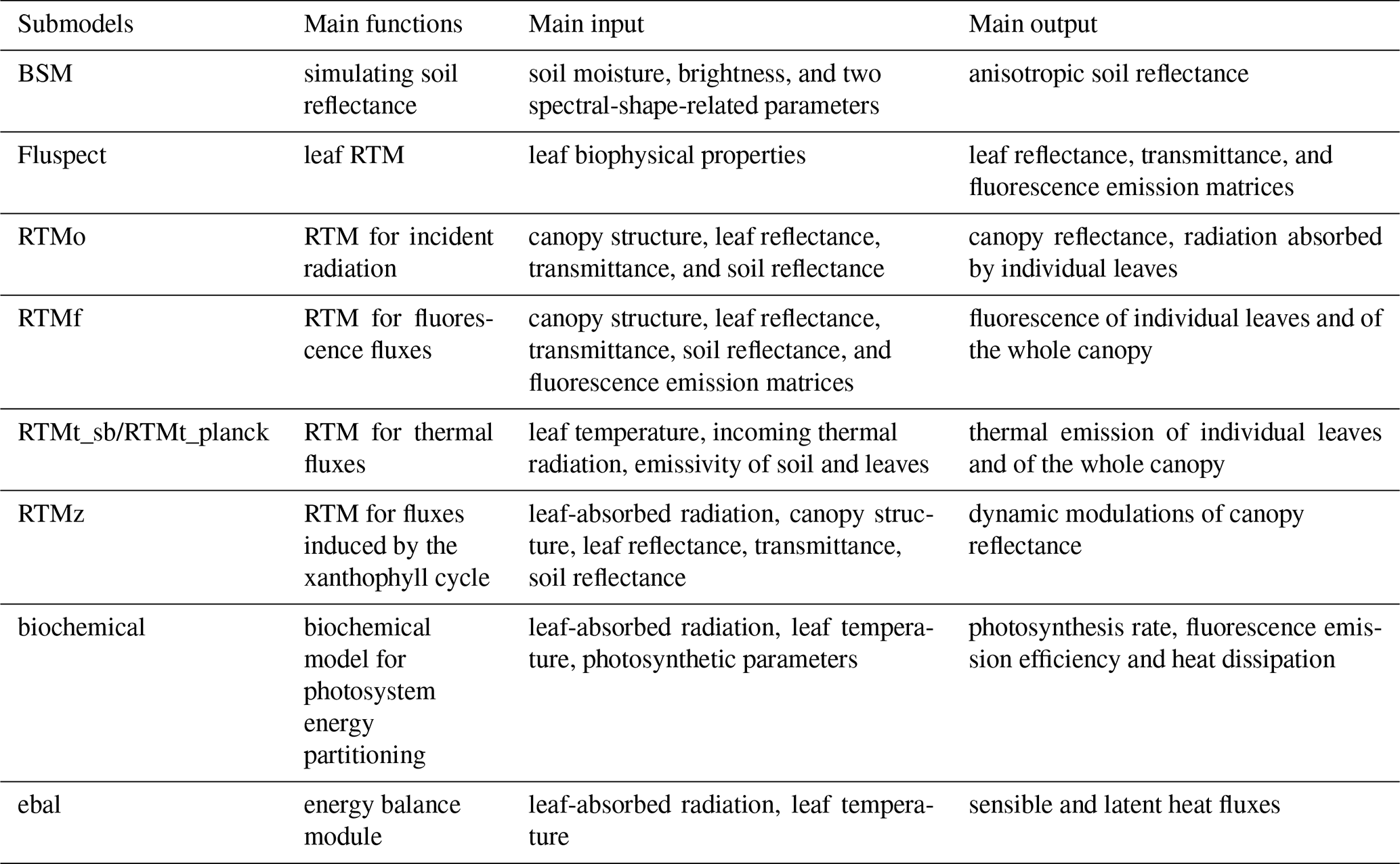
The model code at the highest hierarchical level, SCOPE, calls submodels which operate in series. The main submodels are listed in Table 1. Besides the listed submodels for radiative transfer and energy balance, SCOPE requires functions for input, output, and some supporting functions (such as Planck's equation). Therefore, all the functions used in SCOPE can be organized into four types: (1) RTMs, (2) modules for energy balance, (3) input–output functions, and (4) supporting functions.
2.3.1 RTMs
SCOPE includes seven RTMs, which together simulate the spectrally resolved radiance emanating from the vegetation: one for the soil (BSM, only available in SCOPE 2.0, Verhoef et al., 2018; Yang et al., 2020b), one for the leaf (Fluspect, Vilfan et al., 2016, 2018), and five for the whole stand, i.e. the combined system of soil and foliage. They include one RTM for incident radiation from the Sun and the sky (RTMo), two for thermal radiation emitted by the soil and vegetation (RTMt_sb and RTMt_planck), one for chlorophyll fluorescence (RTMf, van der Tol et al., 2009; Van der Tol et al., 2019), and one for the dynamic modulations of leaf reflectance and transmittance due to pigment changes in the xanthophyll cycle (RTMz, only available in SCOPE v1.70 or later, Vilfan et al., 2018).
Four types of fluxes are involved in the radiative transfer processes, namely a direct solar flux, two hemispherical (semi-isotropic) diffuse fluxes (up- and downward), and a flux in the direction of viewing. Following the Kubelka–Munk theory, the radiative transfer in the vertical direction is expressed with a set of linear differential equations (Verhoef, 1984). These equations are solved either with analytical or numerical approaches. This four-stream radiative transfer theory is applied in SCOPE, and analytical solutions to the radiative transfer problems are essentially based on the approach given in Verhoef (1984) and Verhoef (1985). SCOPE 2.0 employs an updated unified four-stream radiative transfer theory for multi-layer vegetation canopies and uses different solutions for the radiative transfer problems. A complete derivation of the solutions is given in Yang et al. (2020c).
2.3.2 Energy balance module
The energy balance module in SCOPE minimizes the energy balance closure error eebal,
for all leaf and soil elements by iteratively updating their temperature. In this equation, Rn is the net radiation, H the sensible heat flux, λE the latent heat flux, and G the ground heat flux (zero for leaf elements), all in W m−2. In the energy balance, chemical conversions (photosynthesis and respiration) and fluorescence are neglected.
The net radiation is obtained after spectral integration of the radiative transfer modules for incident radiation (RTMo) and internally generated thermal radiation (RTMt). The radiative transfer for incident radiation is computed before the energy balance closure loop, while the internally generated thermal radiation is calculated within this loop because of its dependence on leaf and soil temperatures. The sensible and latent heat fluxes are calculated with an aerodynamic resistance scheme, where resistances for the leaf and soil boundary layer, the vegetation layer, and the atmospheric surface layer apply. The aerodynamic resistances depend on atmospheric stability, wind speed, and surface roughness (van der Tol et al., 2009). For latent heat flux of leaves, a stomatal resistance is calculated with a combined photosynthesis and stomatal model (Van der Tol et al., 2014), while for the soil, a surface resistance applies which is either a pre-defined input or an empirical function of soil moisture.
2.3.3 Leaf biochemical model
The biochemical model simulates the energy partitioning into fluorescence, heat, or photochemistry in photosystems (Maxwell and Johnson, 2000; Van der Tol et al., 2014). It is based on a conventional photosynthesis model of Collatz et al. (1991) for C3 and Collatz et al. (1992) for C4 vegetation, in which photosynthetic rates (or photosynthetic light-use efficiency) are simulated as a function of leaf temperature, ambient radiation levels, intercellular CO2 concentrations Ci, and other leaf physiological parameters (e.g. photosynthetic pathways, maximum carboxylation rate Vcmo). A difference with some other canopy-scale models (e.g. BEPS) is that SCOPE applies the photosynthesis models at leaf level (disaggregated), whereas many other models apply these models at aggregated (big-leaf or Sun-shade two-leaf models) scales.
Van der Tol et al. (2014) established empirical relationships between fluorescence emission efficiency and photosynthetic light-use efficiency under various environmental conditions by using active fluorescence measurements. With these relationships, the fraction of the absorbed radiation by a leaf emitted as fluorescence and dissipated as heat can be simulated.
2.3.4 Interactions among the submodels
Figure 1 is a schematic overview of the SCOPE model structure, which also shows the connections among the submodels. A full list of input parameters is provided in Table 2. A simulation with SCOPE starts with calculating soil reflectance (BSM), the leaf reflectance, and transmittance and fluorescence emission excitation matrices (Fluspect). These simulations of soil and leaf optical properties, together with canopy structure and irradiance, are the input of canopy RTMs. The submodel for radiative transfer of solar and sky radiation (RTMo) takes leaf optical properties and soil reflectance as input and outputs canopy reflectance and radiation fluxes including the net absorbed solar radiation by soil and leaves. RTMf takes the leaf fluorescence emission excitation matrices and the radiation fluxes as input and simulates canopy fluorescence.
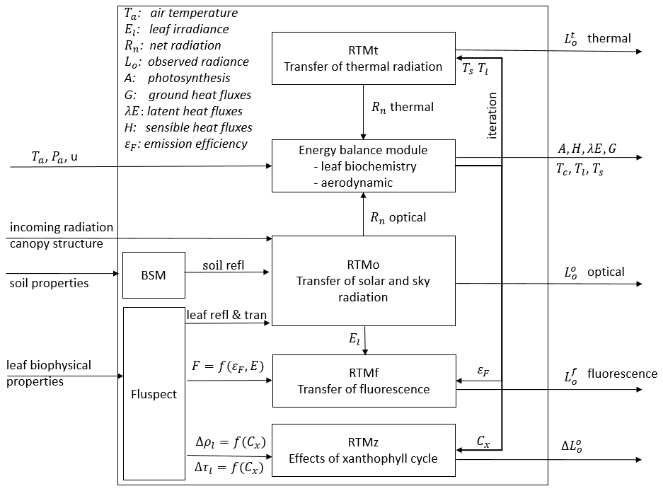
Figure 1Schematic overview of the SCOPE model structure. For a complete list of input data, see Table 2.
The radiative transfer of emitted thermal radiation relies on the temperatures of soil and leaves, which are not known a priori. For this reason, the thermal radiative transfer model is carried out in the energy balance closure loop as described in Sect. 2.3.2. For the purpose of computational efficiency, the radiative transfer of emitted thermal radiation is carried out in broadband in this loop by using RTMt_sb. The letters “sb” denote the use of the Stefan–Boltzmann law to describe the spectrally integrated radiance from a leaf or soil in terms of its temperature. Leaf temperature is also used together with the radiation absorbed by leaf chlorophyll pigments and other leaf physiological parameters to simulate photosystem energy partitioning in the biochemical model (Van der Tol et al., 2014). The energy balance residual is used to update the initial estimate of temperature of each element.
After energy balance closure, the thermal radiation fluxes are simulated as spectrally resolved in the observation direction by using RTMt_planck, where “planck” denotes the use of Planck's law to describe the spectrally resolved radiance from a leaf or soil in terms of its temperature. The radiative transfer of the emitted fluorescence is simulated with RTMf. This module uses the radiative fluxes interacting with leaves as simulated with RTMo, and the fluorescence emission matrices simulated with Fluspect, to simulate leaves' fluorescence emission, which is aggregated to canopy fluorescence signals. Finally, the effect of (small) changes in reflectance and transmittance due to the illumination and temperature-dependent xanthophyll epoxidation state are simulated with RTMz.
2.4 Model inputs and outputs
2.4.1 Input variables for soil, vegetation, and meteorology
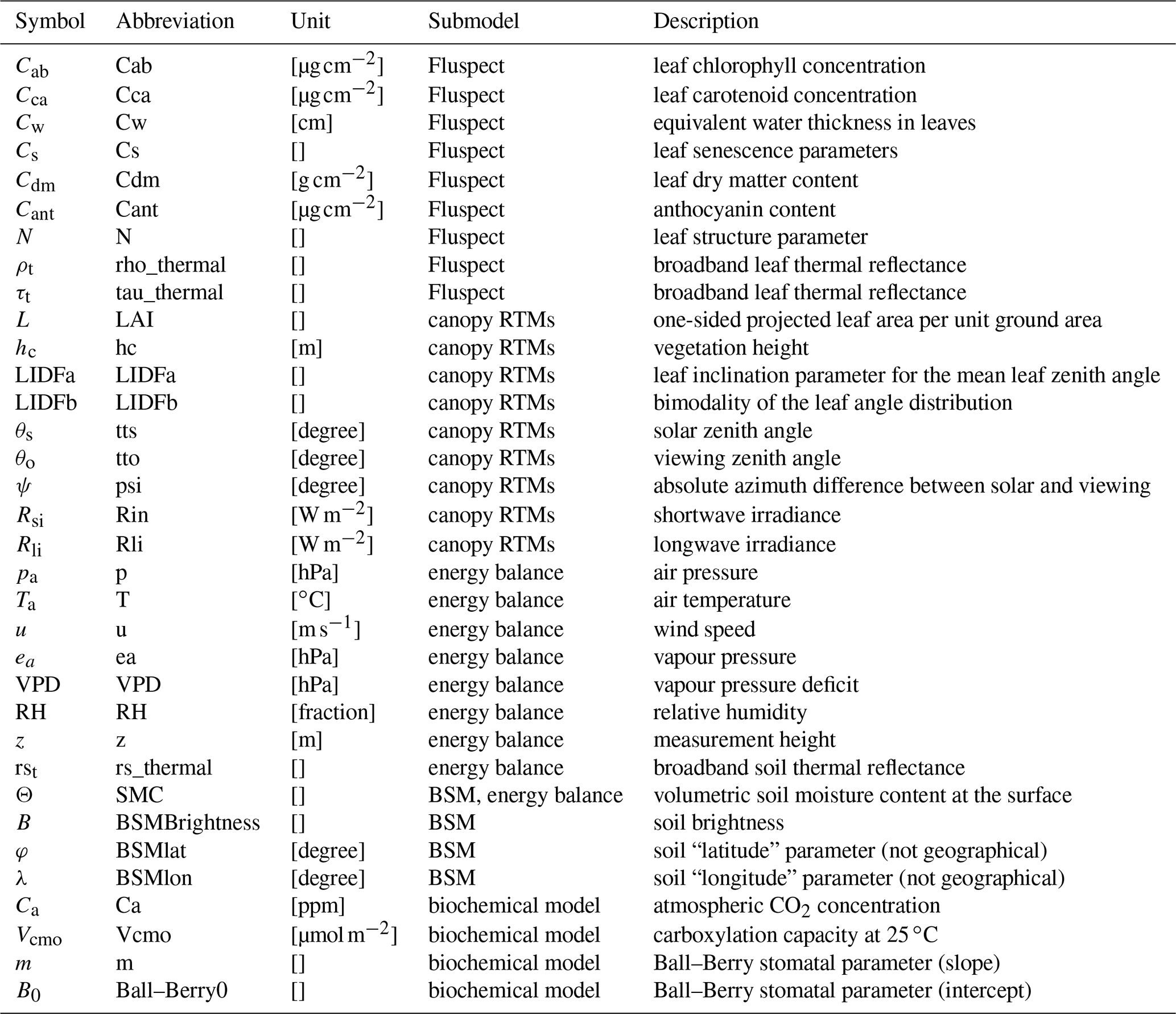
The inputs of the SCOPE model comprise soil, leaf, and canopy properties as well as Sun–observer geometry and meteorological conditions. Besides the intermediate variables, which are passed between the submodels, the main input variables of SCOPE are given in Table 2.
Leaf biophysical and biochemical parameters characterize leaf pigment, water, and dry matter contents, which determine leaf optical properties. Canopy structural parameters describe the arrangement of the leaves in the canopy. Sun–observer geometry is determined by the Sun and observer's zenith angles and their absolute azimuth difference. Both the canopy structural parameters and Sun–observer geometry strongly affect remote sensing signals observed above the canopy.
The meteorological inputs for SCOPE include the typical synoptic weather variables of air temperature, humidity, wind speed, and air pressure, and the concentrations of oxygen and carbon dioxide. All these inputs are required close to the Earth's surface. The height above the surface of the terrain for which they are specified must be given in the input, as input z, typically 2.5 times the vegetation height. Thus, z is not the height of the terrain above sea level but rather the height above the terrain at in surface layer, where the wind profile is logarithmic. The value of z must be given in the input as it is used to calculate the aerodynamic roughness of the surface.
2.4.2 Input irradiance for the atmosphere boundary condition
In addition to the variables listed in Table 2, SCOPE requires the radiative properties of the atmosphere as an upper boundary condition. They can be provided in two different ways.
The first option is to provide irradiance at the bottom of the atmosphere (BOA) in the form of a file with two columns representing the spectra of direct solar irradiance Esun and diffuse sky irradiance Esky [W m−2 ], respectively. These spectra could either be measured in the field or generated with an atmospheric RTM (e.g. MODTRAN, Berk et al., 1999). Using an atmospheric RTM has the disadvantage that Esky may not be accurate, because Esky depends also on the surface (canopy) reflectance in the surroundings, which may not be known a priori in the atmospheric radiative transfer simulation. Therefore, if the surface reflectance assumed in the atmospheric radiative transfer simulation largely differs from the canopy reflectance produced by SCOPE, errors in Esky occur.
The second and preferred option is using an atmospheric RTM to generate some optical properties of the atmosphere rather than the direct output of Esky and Esun. The optical properties should include the following coefficients:
-
Escos (θs), the product of the solar irradiance at the top of the atmosphere (TOA) and the cosine of the solar zenith angle; this product is the irradiance at TOA projected on the surface (W m−2 );
-
ρdd, the diffuse reflectance of the atmosphere (i.e. the spherical albedo);
-
τss, the direct atmospheric transmittance in the direction of the Sun;
-
τsd, the diffuse atmospheric transmittance for solar incidence; and
-
La, the thermal emission by atmosphere at BOA towards the surface (W m−2 ).
The coefficients listed can be extracted from MODTRAN simulations by using the T18 system, which is described in detail in Verhoef et al. (2018). A database of the optical coefficients for several typical atmospheric conditions is provided together with the SCOPE model. With these coefficients, SCOPE can simulate the BOA direct and diffuse irradiance spectra in the module RTMo with consideration of surface–atmosphere interactions. The BOA irradiances Esun and Esky are calculated in the function RTMo as
where rsd and rdd are the surface reflectance for direct and diffuse incoming radiation, respectively, and Ls the thermal emission by the (vegetated) surface (). All of them are simulated with SCOPE. The overbars denote the spectral averaging to the SCOPE resolution (1 nm in the visible–near infrared, VNIR). Note that τss and ρdd are aggregated to the SCOPE resolution separately, but also the product τssρdd, in order to accommodate spectral correlation effects in the finite bands. The coupling with the atmosphere is described in detail in Verhoef et al. (2018) and Yang et al. (2020b).
Finally, SCOPE offers the possibility to provide additional values for the spectrally integrated irradiance (direct solar radiation Esun plus Esky) over the ranges from 0.4 to 2.5 µm and 2.5 to 50 µm. These are the input fields Rsi and Rli, respectively. However, it is not necessary to specify these inputs, because the broadband irradiances Rsi and Rli are already calculated internally as the integral of the irradiance spectra. If the values for these two inputs are specified, then the solar and sky irradiance spectra Esun plus Esky are linearly scaled (each by the same factor so that the ratio remains unaltered) in the two spectral regions separately to match the values provided for Rsi and Rli. This option can be useful if time series of synoptic weather data are used as input, and if it is computationally not feasible to carry out atmospheric radiative transfer simulations for every time step separately. For coupled surface–atmosphere simulations, this is not recommended, because of obvious inconsistencies between SCOPE and the atmospheric model. In that case, the input fields for Rsi and Rli must be left blank.
2.4.3 Model outputs
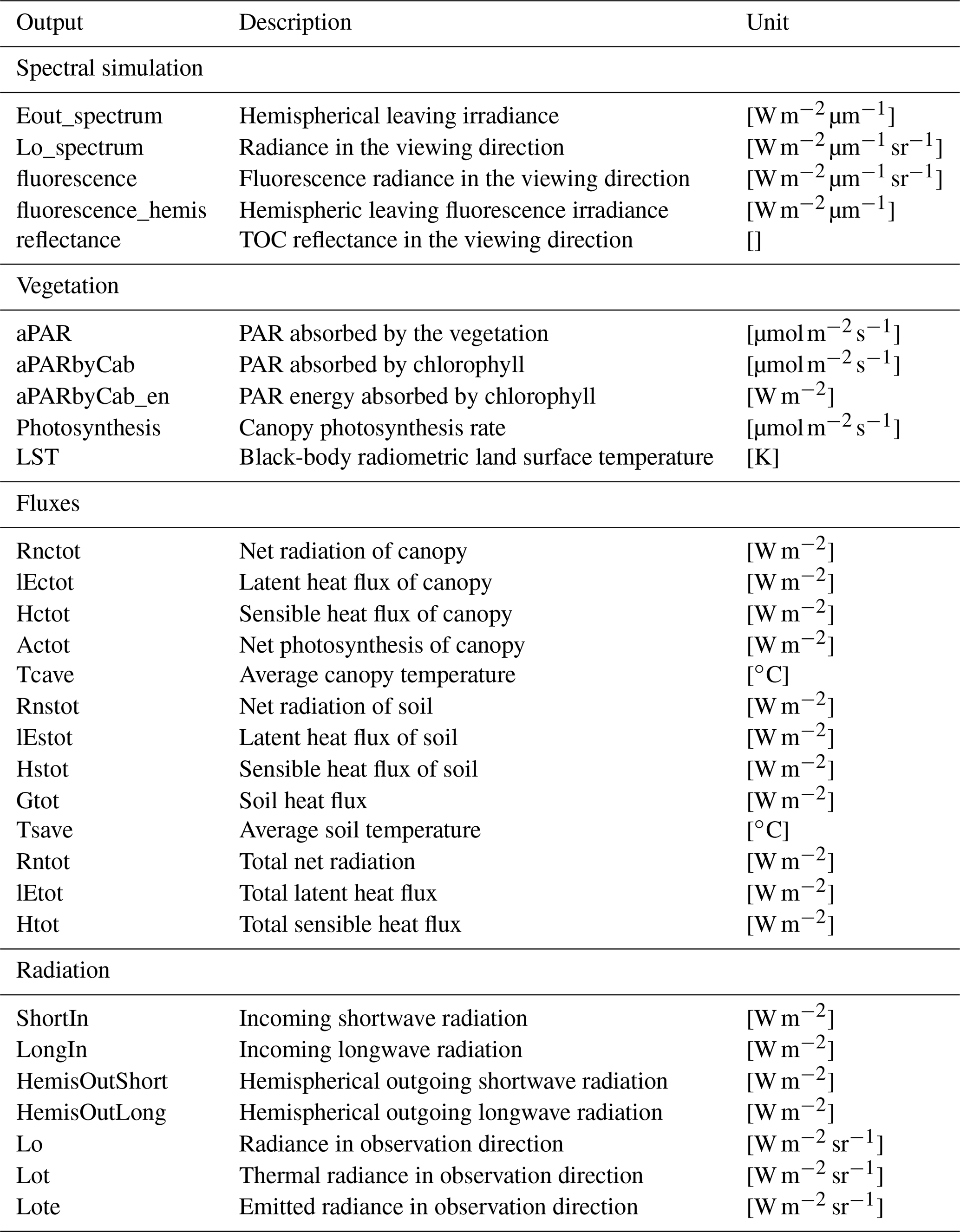
In Table 3, the main outputs of SCOPE are listed. The general output of SCOPE includes (1) spectral simulations of radiance in the viewing direction and upward flux for the whole upper hemisphere from optical to thermal domain including fluorescence; (2) radiation budget, such as incoming and outgoing radiation for shortwave from 0.5 to 2.5 µm and longwave from 2.5 to 50 µm; (3) fluxes such as sensible heat, latent heat, and the ground heat flux for canopy, soil, and the combined system; and (4) canopy absorption, such as absorbed PAR by chlorophyll. Most of the stored outputs of SCOPE are for the whole canopy, although similar variables of leaves are also computed internally in SCOPE. Some intermediate variables, e.g. leaf-absorbed PAR by chlorophyll and fluorescence spectra, are simulated but not stored as the final outputs.
3.1 Implementation of the BSM soil reflectance model
In the first published version of SCOPE, the soil reflectance spectrum was an input variable. The users should either provide a measured soil spectrum or select one from the soil reflectance library incorporated in the SCOPE model. In SCOPE 2.0, we provide the users the option to simulate soil reflectance thanks to the implementation of a soil reflectance model.
The BSM model simulates the isotropic soil reflectance. This model is based on an empirical reflectance model of dry soil (Verhoef et al., 2018; Jiang and Fang, 2019) and incorporates the effects of soil moisture by using the water film coating approach (Ångström, 1925; Yang et al., 2020b). To simulate reflectance of dry soil, the model requires soil brightness (B) and two spectral-shape-related parameters (φ and λ) as inputs. Soil moisture is necessary for simulating wet soil reflectance.
Figure 2 shows the effects of the four parameters on soil reflectance. It is evident that soil brightness only affects the “intensity” of soil reflectance and the “shape” of soil reflectance is controlled by φ and λ. Soil moisture affects reflectance intensity over all wavelengths but reflectance at the water absorption bands is more sensitive to soil moisture. Soil moisture effects on reflectance are considerably similar to the effects of soil brightness, and soil is dark when it is wet as explained in Lekner and Dorf (1988).
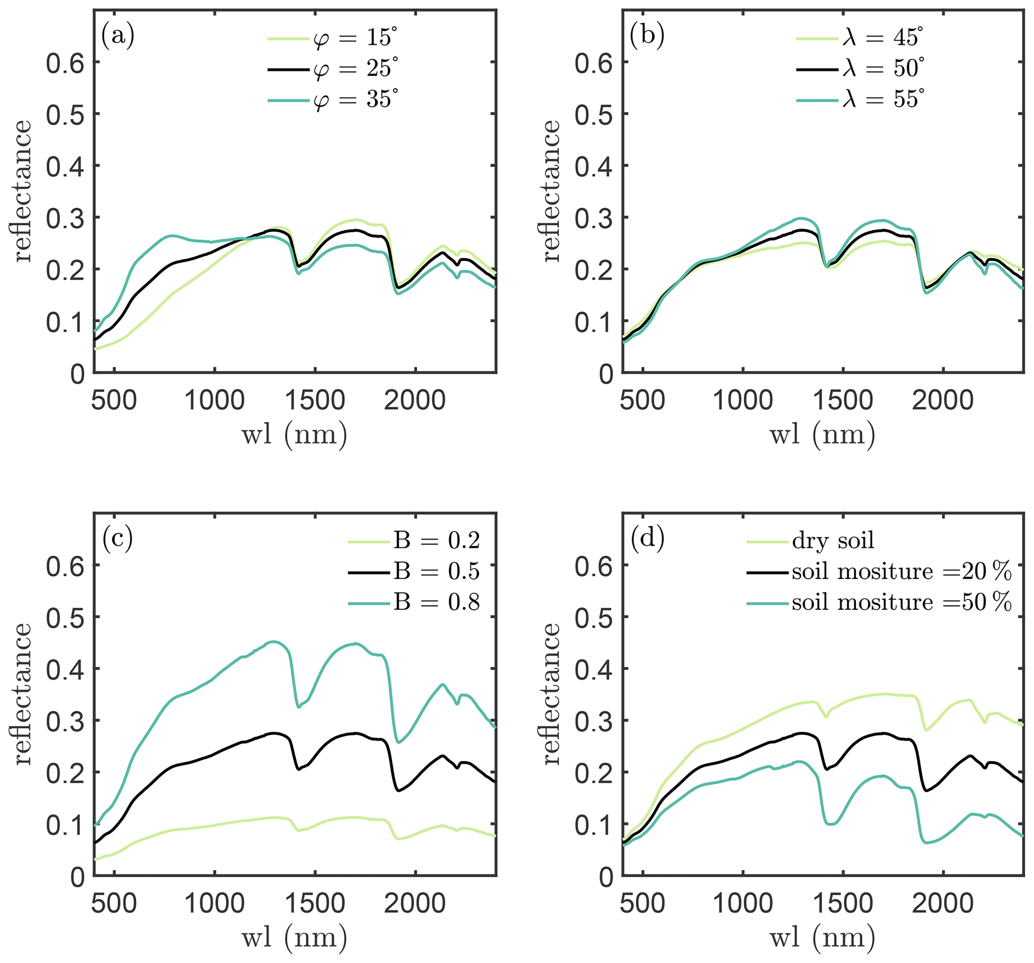
Figure 2Reflectance simulations with the BSM model. The black curves in each panel are the same simulation.
3.2 Inclusion of dynamic reflectance induced by the xanthophyll cycle
A new feature in SCOPE 2.0 is modelling the photochemical reflectance dynamics induced by the xanthophyll cycle at both leaf and canopy levels. In the original leaf RTM Fluspect (Vilfan et al., 2016), leaf optical properties are determined by leaf biophysical properties. However, in natural conditions, the xanthophyll cycle that is involved in photo-protection mechanisms under excess light can provoke a change in reflectance and transmittance as the composition of the pigment pool is regulated. Changes in the de-epoxidation state (DEPS) of xanthophyll cycle pigments (e.g. violaxanthin and zeaxanthin) can be observed as changes in the leaf absorption of light with wavelengths between 500 and 570 nm. These spectral changes can be a good remote sensing indicator of the photosynthetic efficiency. The photochemical reflectance index (PRI, ) proposed by Gamon et al. (1992) is a example of a measure for the effects of xanthophyll cycle pigments on the reflectance. It takes changes in reflectance at 531 nm to estimate DEPS with reflectance at 570 nm as a reference to correct changes in reflectance induced by other factors, such as Sun–observer geometry.
Vilfan et al. (2018) incorporated the effects of the xanthophyll cycle on leaf optical properties in Fluspect and developed the Fluspect-CX model. The main idea of Fluspect-CX is to use in vivo specific absorption coefficients for two extreme states of carotenoids, representing the two extremes of the xanthophyll de-epoxidation. A “photochemical reflectance parameter” (Cx) is employed to describe the intermediate states as a linear mixture of these two states. Cx controls the specific absorption coefficient of carotenoids in a leaf and thus affects leaf reflectance and transmittance.
The propagation of changes in leaf reflectance and transmittance induced by the xanthophyll cycle to TOC reflectance is carried out with RTMz, which is largely similar to RTMf in the sense that both the xanthophyll cycle and fluorescence emission lead to small changes in (apparent) reflectance but for different spectral regions (i.e. 500–570 and 640–850 nm, respectively). RTMf and RTMz take fluorescence emission efficiency and Cx (simulated from the leaf biochemical model), respectively, as inputs, of which the magnitudes vary among individual leaves due to their ambient light intensities, temperature, etc. Figure 3 depicts an example of the effects of Cx on the leaf and canopy reflectance as simulated by SCOPE 2.0 with the default model inputs. Although the effects on canopy reflectance seem small, they could be helpful for monitoring the variation in DEPS.
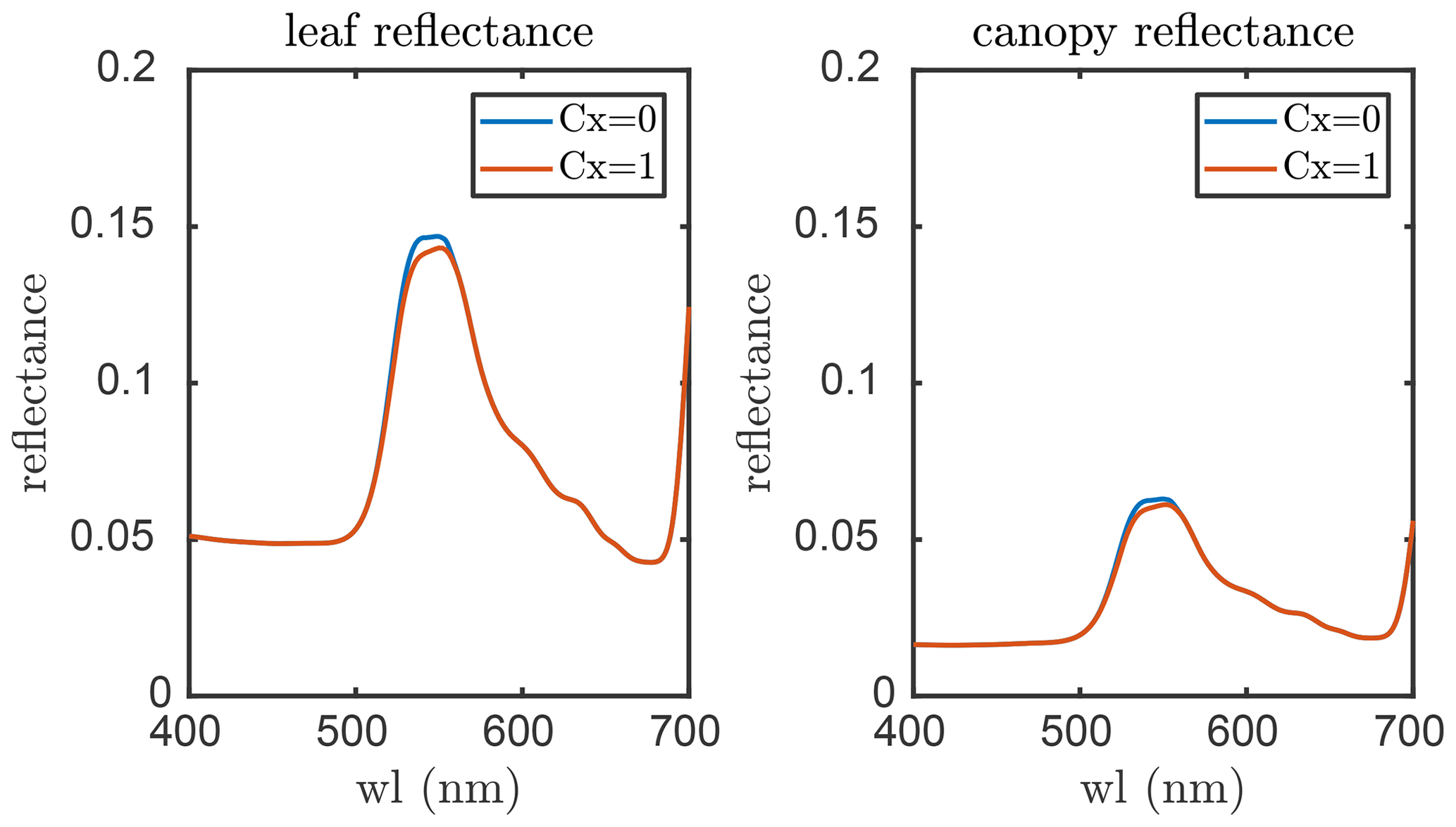
Figure 3The effects of the xanthophyll cycle on leaf and canopy reflectance simulated with SCOPE 2.0. Cx is a factor for the de-epoxidation state (DEPS) of xanthophyll cycle pigments.
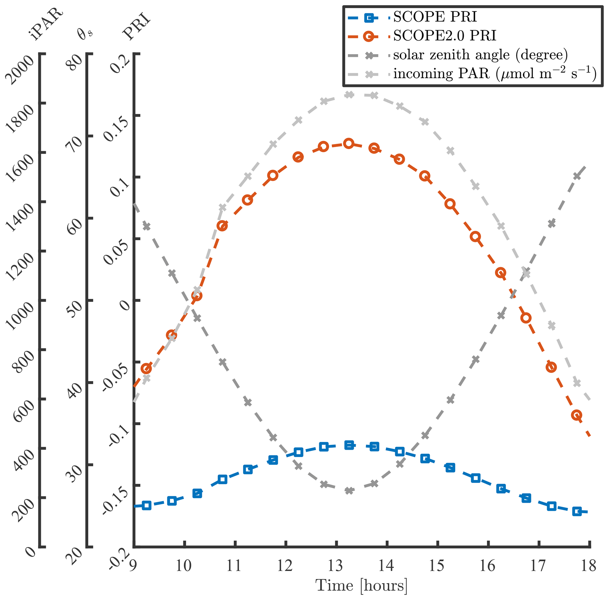
Figure 4 compares simulations of PRI in a day with SCOPE and SCOPE 2.0. In these simulations, the default model inputs are used except for the incoming radiation and solar zenith angles. The values of incoming radiation and solar zenith angles (θs) are assigned according field measurements presented in Yang et al. (2020a) (i.e. on day 232 of the dataset in the referred paper). The comparison demonstrates that the inclusion of dynamic reflectance induced by the xanthophyll cycle has a clear impact on the simulation of diurnal changes in PRI. In SCOPE, diurnal variation of PRI is mainly regulated by Sun–observer geometry, since leaf biophysical properties and canopy structure are kept unchanged in a day. Because the bidirectional reflectance distribution function (BRDF) effects on reflectance at 531 and 570 nm are similar, they cancel out in PRI, and the diurnal variation of PRI simulated with SCOPE is small. Compared with SCOPE, SCOPE 2.0 considers the changes in leaf pigment pool induced by the xanthophyll cycle in response to the variation of incoming radiation besides the BRDF effects. The excessive incoming radiation during midday leads to larger Cx values than in the morning and afternoon, and higher afternoon than morning temperatures to higher afternoon Cx, and thus more significant diurnal variation of PRI.
3.3 Adaption of the RTMs for multi-layer canopies
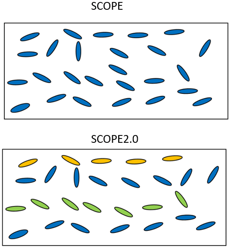
The original SCOPE model assumes that vegetation canopies are vertically homogeneous and horizontally infinite, as its radiative transfer routines are based on the classical 1-D SAIL model (Verhoef, 1984). The vertical heterogeneity of leaf biophysical and biochemical properties may have a large effect on the bi-directional reflectance, fluorescence, and photosynthesis of vegetation canopies. To allow simulations of vertical heterogeneous canopies, Yang et al. (2017) modified the RTMs in SCOPE and developed a new branch of SCOPE, called mSCOPE. SCOPE 2.0 incorporates the essence of mSCOPE on radiative transfer modelling and adapts the capability to simulate reflectance, fluorescence and photosynthesis of vertically heterogeneous canopies (as illustrated in Fig. 5). In comparison with the original SCOPE, SCOPE 2.0 accepts vertical profiles of leaf properties (such as chlorophyll content) as inputs. This is done via a table in which optical properties can be specified for user-defined LAI intervals. If single values of the Fluspect parameters in Table 2 are provided, the model will assume the canopy is vertically homogeneous. The true heterogeneity of leaves within a vegetation canopy may be too large to fully implement in the model. Thus, a simplification of the canopy may be needed: two- or three-layer representations are most common. For example, forests usually have understorey and overstorey, and crops at the senescent stage have two or three distinct layers with brown or green leaves. However, it is noted that more layers are possible in SCOPE 2.0 for specific purposes as shown in Yang et al. (2017).
RTMs in SCOPE 2.0 remain structurally the same with the original SCOPE. However, a more general solution of the radiative transfer problems is used. Compared to the classic SAIL analytical solution, SCOPE 2.0 (and mSCOPE) employs the adding method to solve the radiative transfer problems. The application of the adding method for TOC reflectance simulation is given in Verhoef (1985). Yang et al. (2017) extended this method to calculating the radiative flux profiles in the canopy. The procedure is summarized as follows: (1) divide the vertical layer into n thin homogeneous layers; (2) start from the bottom homogeneous layer, calculate the surface reflectance of the combined system of the bottom surface (e.g. soil) and this layer; (3) add a new homogeneous vegetation layer above the surface of the previous system in step 2, and calculate the surface reflectance of the new system; (4) repeat step 3 until all homogeneous layers are added. (5) Once the surface reflectance at each vertical level is obtained, the fluxes profile can be computed from top to bottom, given the incident fluxes at top of the canopy. For the radiative transfer of fluorescence and thermal radiation, the emission from leaves and soil should be included as extra radiation sources besides the incident fluxes at the top of the canopy. In SCOPE 2.0, the value of n is set as 10 times the LAI rather than a fixed value of 60 in mSCOPE, because this ensures the LAI of one elementary layer is small enough (i.e. LAI of a thin layer, iLAI <0.1), and the use of less elementary layers improves the computational efficiencies of the RTMs.
3.4 An alternative way to estimate the ground heat flux
In SCOPE, the ground heat flux is calculated for the sunlit and shaded soil (the heat storage changes in the canopy are not considered). In the original SCOPE model, this was either a constant fraction of 0.35 of the net radiation on the soil or calculated with the force restore method of Bhumralkar (1975). SCOPE 2.0 offers an alternative way to estimate the ground heat flux as a function of the soil temperature time series with the method of Wang and Bras (1999). The ground heat flux is determined by the gradient of soil temperature in the profile underneath the soil surface. The subsurface is outside the model domain of SCOPE, and therefore the soil temperature gradient is not simulated. However, this vertical gradient may equivalently be expressed the by the half-order time derivative of the surface temperature (Wang and Bras, 1999). This enables the estimation of G from the time history of the surface temperature:
where T is the soil temperature at time s, Γ [J m−2 s K−1] is the thermal inertia of the soil, calculated from physical properties of the soil:
where cs is the volumetric heat capacity of the soil [J kg−1 K−1], ρs the soil bulk density [kg m−3], and λs [J m−1 s−1 K−1] the heat conductivity of the soil. In SCOPE 2.0, a solution derived for a discrete time series of temperatures by Bennett et al. (2008) (Eq. A3 therein) was adopted:
This approach is only meaningful if consecutive simulations are carried out in a time series, in which the diurnal variation of temperature is reproduced (at least one simulation per 3 h time step). The approximation of G=0.35Rns should be used for cases in which the state of the soil heat reservoir cannot be known, for example, if simulations are carried out for pixels in a satellite image taken at a single moment in time.
3.5 Improvements in energy balance closure
The energy balance loop starts by simulating the radiative transfer of internally generated radiation with initial estimates of component temperatures, followed by the calculation of aerodynamic and stomatal resistances (and photosynthesis), and the fluxes H, λE, and G. Finally, new estimates of the component temperatures are calculated from the value of the energy balance closure error (ΔE) per leaf and soil element. Newton's method is used to estimate the new temperatures, which are the starting point for the next iteration in the loop.
where is the first derivative of the energy balance closure error to temperature, and W is a weighting for the step size. The derivative is estimated analytically:
Equation (6) is a linearization of the relation between temperature and energy balance error. This linearization is estimated analytically, which is much faster than calculating the derivative numerically. In the estimate, it is assumed that the incident irradiance on the leaves (or soil) does not change. This is an approximation. The internally (in the canopy) generated incident irradiance depends on the temperature of the neighbouring leaves, which is updated in the next iteration step as well. Further, it is assumed that the resistances ra and rs do not change between iteration steps. This is an approximation as well, as both depend on leaf and soil temperature. Although these interactions cannot be resolved analytically, Eq. (6) is a sufficiently accurate approximation of the first derivative to obtain rapid energy balance convergence. Iterations continue until the maximum absolute closure error of all leaf and soil elements is less than 1 W m−2, and this is usually achieved in less than 10 iteration steps. If energy balance closure is not achieved after 10 steps, then the weighting coefficient W is gradually decreased from 1 (i.e. smaller update steps) to avoid the updated temperatures bouncing around the solution.
In earlier versions of SCOPE, a similar equation to Eq. (6) has been used to update temperature in the energy balance loop. However, the partial derivative of latent heat flux to temperature was not included in the equation. The improvement in SCOPE 2.0 has substantially reduced the number of required iterations due to a more complete estimate of the derivative.
3.6 Angular aggregation of sunlit leaves
In the energy balance routine, the number of sunlit leaf elements that are considered is 13 leaf zenith × 36 leaf azimuth times 10×LAI layers, while the number of shaded leaf elements is 10×LAI. Solving the energy budget for all these elements separately means that a closure of energy balance should be achieved for each element and this is computationally demanding. SCOPE 2.0 offers the possibility to simulate the non-radiative energy fluxes, photosynthesis and gas exchange for all inclination and azimuth angles of the sunlit leaves combined (the 'lite' option). This involves an aggregation (weighted averaging) of net radiation over all leaf angles, before entering the energy balance loop. One effective leaf for the 13×36 sunlit leaf classes is used for each layer. The resulting number of elements is 10×LAI for the sunlit leaves and 10×LAI for the shaded leaves. This significantly reduces the computation time of the energy balance routine.
The consequence of this internal aggregation is that the all sunlit leaves in a layer will have an identical temperature, gas exchange, photosynthesis rate, chlorophyll fluorescence emission efficiency, and latent and sensible heat fluxes, independent of their inclination towards the Sun. Figures 6 and 7 present examples for the effects of the angular aggregation on the profiles of leaf temperature and photosynthesis simulations, respectively. In these simulations, the default model inputs are used. Due to the simplifications in the energy balance and biochemical part in the lite mode, the layer-average temperatures become slightly higher for both sunlit and shaded leaves (Fig. 6). A slight difference in photosynthetic production between the lite-on and lite-off modes can be found for sunlit leaves, but the difference for shaded leaves is negligible (Fig. 6). The photosynthetic production simulation for the whole canopy changes by about 0.7 (4 %) when the lite mode is activated. The differences in leaf temperature and photosynthesis are apparently affected by the incoming radiation, leaf biochemistry, canopy structure, and other model inputs. The implementation of the lite mode might be helpful for estimation of the added value of consideration of various leaf orientations in a canopy in comparison of the simpler one-big-leaf or two-big-leaf models (Dai et al., 2004; Luo et al., 2018).
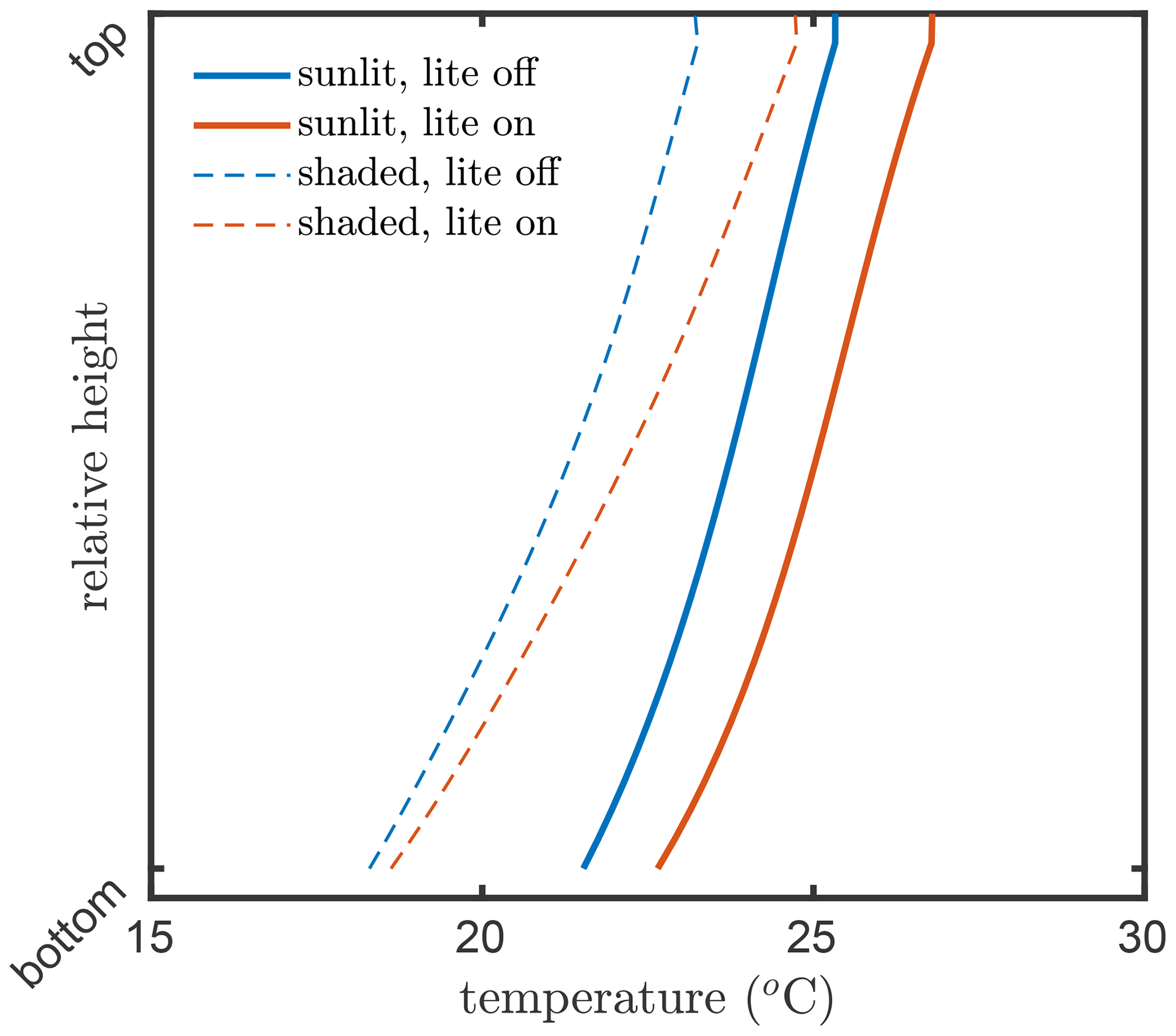
Figure 6Layer-average kinetic temperatures of the leaves in the vegetation canopy simulated by SCOPE 2.0 with the “lite” representation on (red) and off (blue) of the vegetation, for sunlit (solid lines) and shaded (dashed lines) leaves.
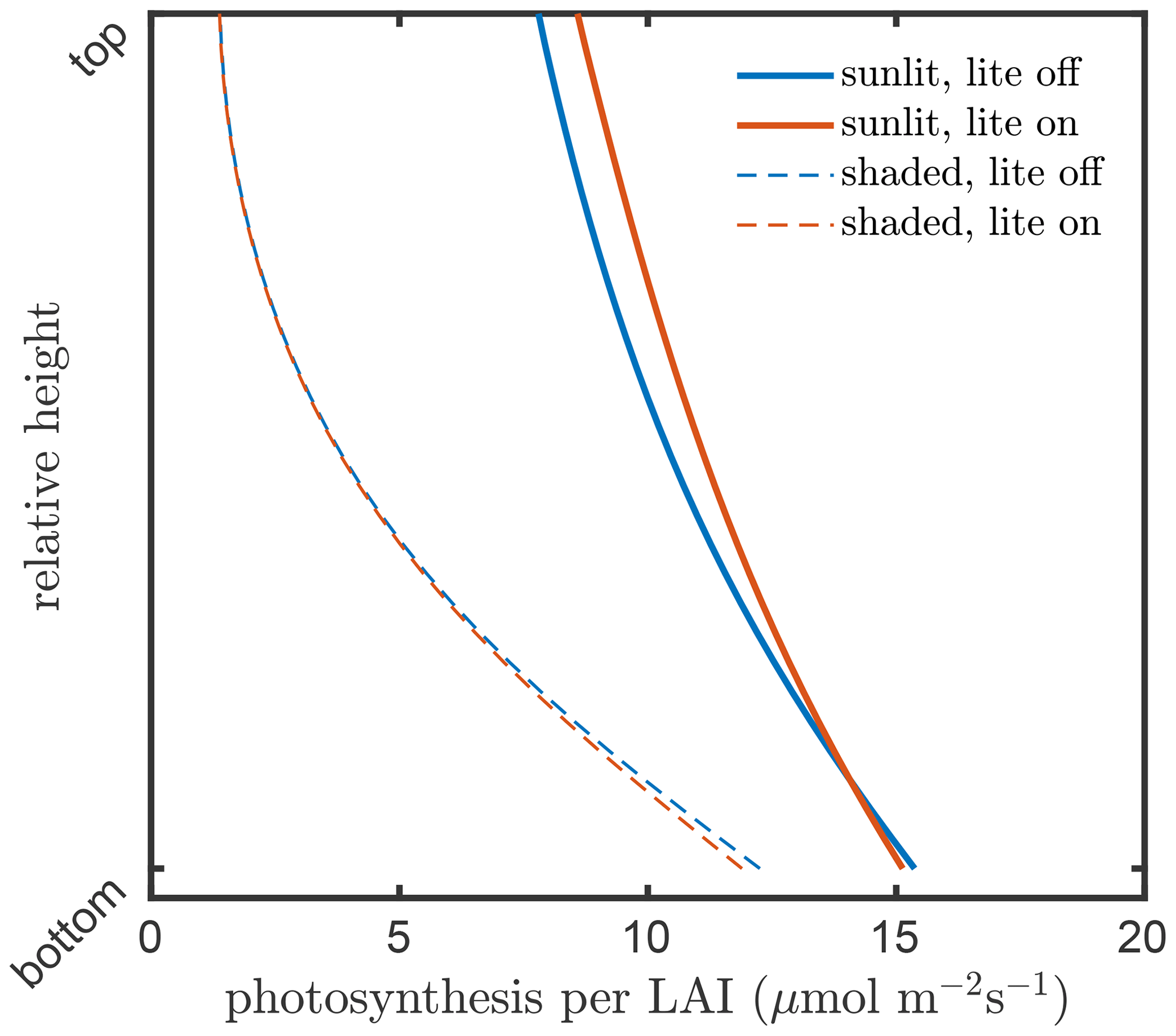
Figure 7Layer photosynthesis per LAI in the vegetation canopy simulated by SCOPE 2.0 with the “lite” representation on (red) and off (blue) of the vegetation, for sunlit (solid lines) and shaded (dashed lines) leaves.
With the lite option switched on, the emitted (thermal and fluorescence) radiation is calculated for layer-average temperature and emission efficiency, respectively, albeit separately for the sunlit and shaded portions. The aggregated layer properties will propagate into the simulation of fluorescence and surface brightness temperature (Tb) as observed above the canopy. Figure 8 presents an example for the effects of the angular aggregation on fluorescence and Tb simulation with the default model inputs. With the default values of the model parameters, the difference in TOC SIF is around 0.1 and around 1∘ in the surface temperature simulation. The difference in radiance is minimal, while the difference in average temperature is relatively higher (compared to the natural spatiotemporal variability). This is not an error but simply due to the non-linear relation between temperature and irradiance in the Planck law. However, the applicability of the lite option depends on specific purposes and the desired accuracy. It is worth noting that the RTMs are all carried out with the original representation of the canopy, thus with 13×36 leaf orientations per layer. This means that the lite mode has no influence on reflectance, net radiation in the optical domain, and absorbed photosynthetically active radiation (APAR) by leaves. Moreover, the directionality and hotspot is still simulated (Fig. 8).
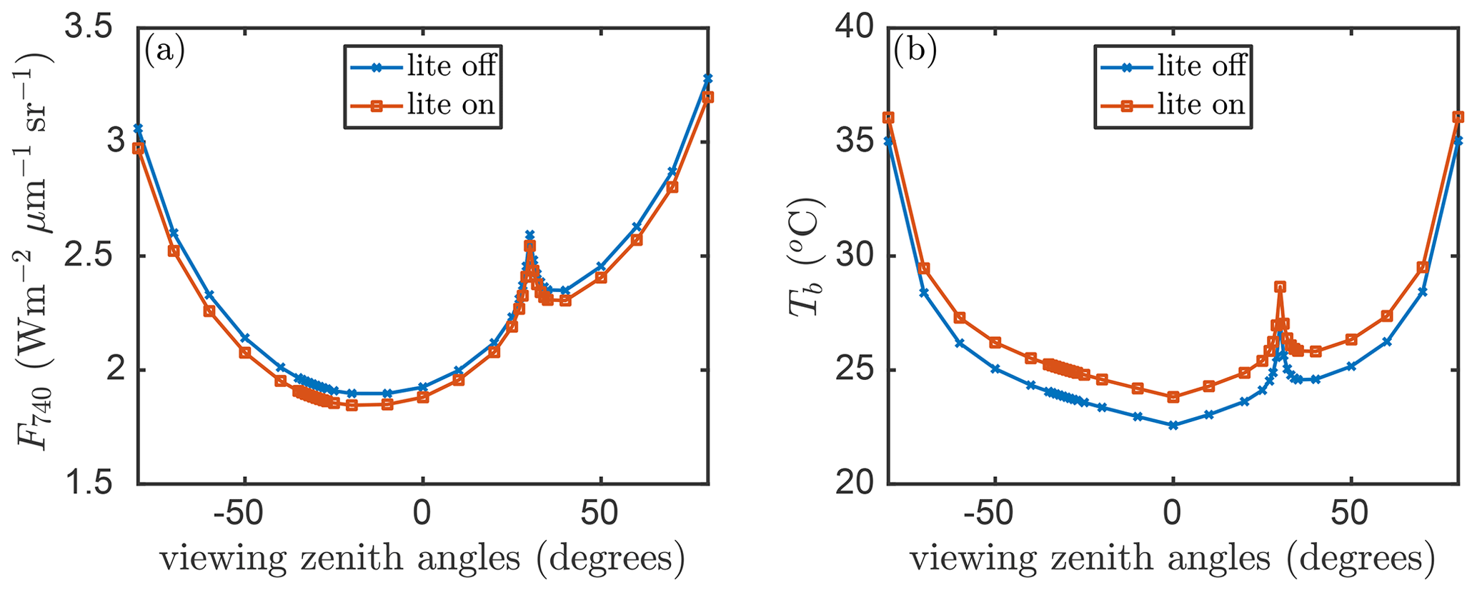
Figure 8(a) Top-of-canopy fluorescence at 740 nm (F740) and (b) surface brightness temperature (Tb) simulated by SCOPE 2.0 with the “lite” representation on (red) and off (blue) of the vegetation versus viewing angles in the principle plane.
3.7 Improvements in the computational efficiency
In SCOPE 2.0, substantial reductions in computation have been achieved compared to SCOPE 1.70 (Table 4). In a test case of 100 scenarios run by SCOPE 2.0 using a regular PC, the computation time is 12.8 % (lite option off) or 7 % (lite option on) of the same 100 scenarios run by SCOPE 1.70. The reduction of computation time is due to (in order of decreasing contribution) (1) a more efficient energy balance closure, (2) more efficient saving of output (initially as binary files, later converted to csv), (3) the overall reduction of the number of layers (from 60 to 10×LAI), and (4) introducing the mSCOPE radiative transfer equations, which allows for a better re-use of earlier calculated quantities. A further factor of 2 in computation time can be achieved when switching off the temperature correction of biochemical parameters (such as Vcmo) with the option “tempcor”, due to a more rapid convergence of the energy balance loop (not shown).
Table 4Breakdown of computation time to the most computationally intensive modules in SCOPE 1.70 and SCOPE 2.0 expressed as seconds per 100 simulations.
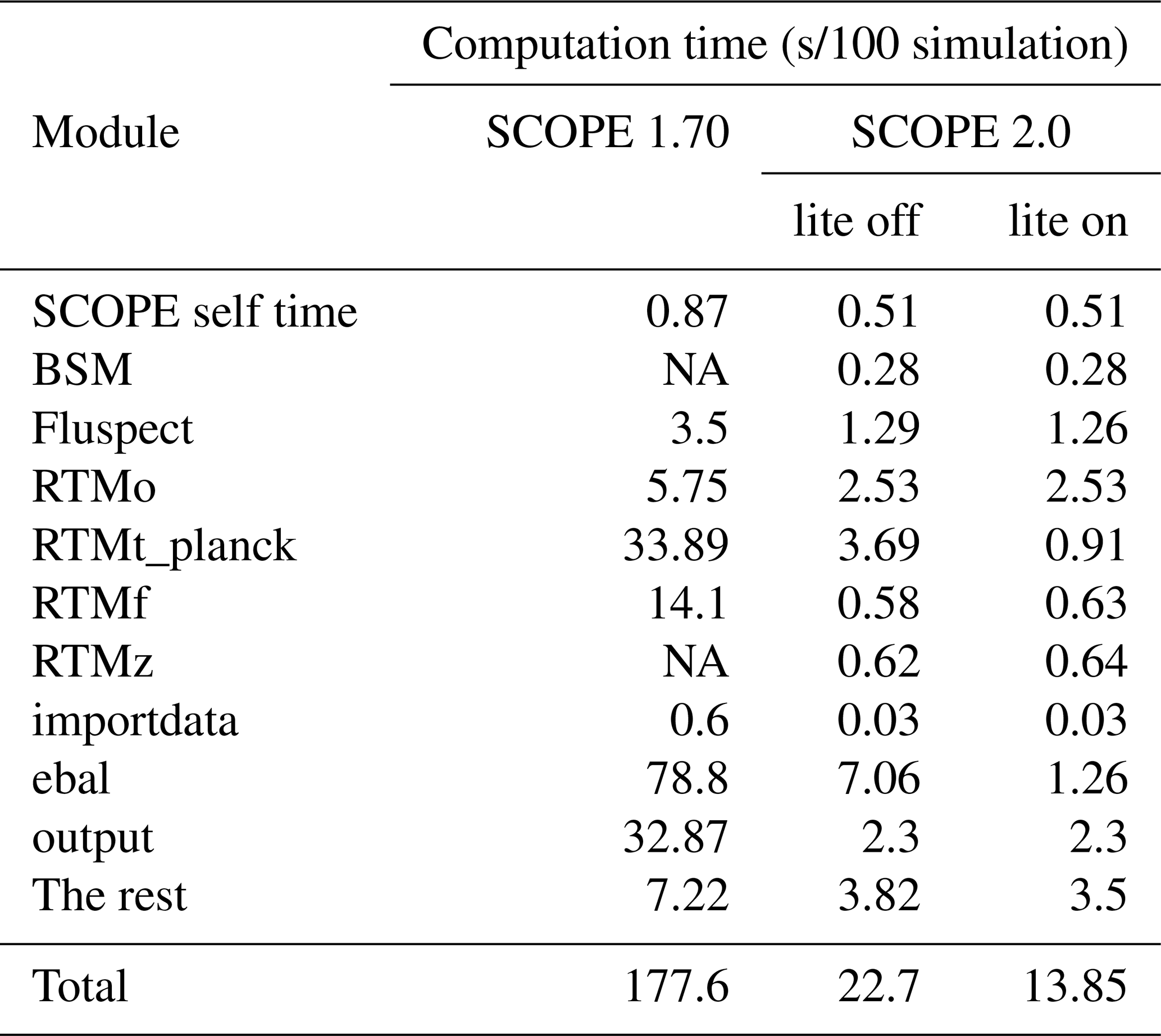
NA – not available
3.8 Additional outputs
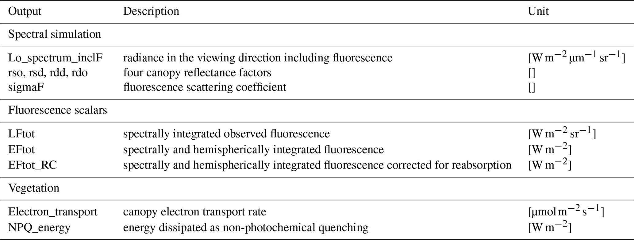
In addition to the output of the original SCOPE model, more model output parameters are produced and stored in SCOPE 2.0, considering users' needs. In Table 5, the outputs available in SCOPE 2.0 but not in the original SCOPE model are presented. Nevertheless, it is worth noting that all the outputs produced in SCOPE 2.0 can also be computed in the original SCOPE with little effort, although they are not stored as outputs.
In the original SCOPE model, TOC reflectance spectral simulation in the viewing direction is provided as an output. It is computed as
where Lo is the radiance in the viewing direction excluding fluorescence contribution, and Esun and Esky the incoming direct solar and diffuse sky irradiance.
In practice, many users do not have measurements of Esun and Esky or atmospheric properties available for inputs but the fraction of diffuse light (fsky). Therefore, we provide the directional reflectance factors of the surface as outputs: rso, rsd, rdd, and rdo. The two-letter subscripts indicate the incident and outgoing fluxes types: d referring to the diffuse fluxes, s referring to the direct solar flux, and o referring to the flux in the viewing direction. These four reflectance factors are independent of the incoming irradiance but are optical properties of the soil–vegetation system. The canopy reflectance in the viewing direction can be estimated as
Furthermore, the radiance in the viewing direction including the fluorescence contribution is provided, which allows computing the apparent reflectance of a vegetation canopy beside the true reflectance.
We include several fluorescence variables as outputs to help to better interpret fluorescence signals in SCOPE 2.0, besides fluorescence at top of canopy. Because fluorescence produced by all photosystems is considered to have a more direct relationship with canopy GPP (Yang and Van der Tol, 2018; Van der Tol et al., 2019), we include it in the outputs. This allows us to compute an important variable: the fluorescence scattering coefficient, which is defined as
where EF is the total emitted fluorescence irradiance by all photosystems, calculated as the canopy integration of the product of absorbed photosynthetically active radiation by chlorophyll, the fluorescence yield, and the (constant) spectral shape of chlorophyll fluorescence. The coefficient σF is sometimes referred to as the “escape probability” in the literature. It can be used to correct the fluorescence for both Sun–observation geometry and reabsorption of fluorescence in the canopy in order to estimate a canopy-effective fluorescence yield (Yang et al., 2020a).
The biochemical model quantifies the energy partitioning into different pathways and computes their light-use efficiencies at leaf scale. The energy partitioning concept is applied to the whole canopy. By taking the weighted average values of the efficiencies of individual leaves, we obtain canopy electron transport rate and non-photochemical quenching (NPQ), which describes the effective photosynthetic light-use efficiency and the effective efficiency of the heat dissipation pathway of the canopy (Maxwell and Johnson, 2000). These variables are direct indicators of the physiological status of the whole canopy.
We presented a significantly improved version of the Soil-Canopy Observation of Photosynthesis and Energy fluxes (SCOPE) model. SCOPE 2.0 simulates the energy balance fluxes of net radiation, sensible and latent heat fluxes, ground heat flux, and photosynthesis, as well as hyperspectral radiance in the optical and thermal domain including the contribution of fluorescence.
The improved computational efficiency and model stability make the model a suitable tool for routine estimation of fluxes and satellite signals, in homogeneous vegetation canopies with an understorey and overstorey, or multi-layer structure. The new features also include the simulation of a subtle change in the reflectance due to the xanthophyll cycle dynamics in the range of 500–600 nm, allowing a better investigation of vegetation physiology under various weather conditions. With the aim for accurate simulations of vegetated land surface processes and remote sensing signals, the models are constantly improved. Some important features, such as canopy clumping effects, crop yield simulation, leaf specular reflection, and soil BRDF effects, are considered as the future directions of SCOPE improvements.
The source code of the model described in this paper is freely available to users via https://doi.org/10.5281/zenodo.4309327 (Van der Tol et al., 2020). Different versions of the model and the details of model developments can be found on GitHub (https://github.com/Christiaanvandertol/SCOPE, last access: 1 May 2021). SCOPE is written in MATLAB and is compatible with versions 2013a and later. A compiled version is available for the MATLAB Runtime Compiler 2019a.
Due to the nature of this research, the data that support the findings of this study can be generated with the presented model using the settings described in the paper.
CvdT and PY designed the model general structure of SCOPE 2.0. WV and PY developed the BSM model and the multi-layer vegetation parameterization. CvdT, PY, and EP wrote the model code and performed the simulations. EP and CvdT wrote the online model documentation. PY and CvdT prepared the manuscript with contributions from all co-authors.
The authors declare that they have no conflict of interest.
Publisher's note: Copernicus Publications remains neutral with regard to jurisdictional claims in published maps and institutional affiliations.
Many users contributed with their feedback and suggestions. Particular thanks are given to Ari Kornfeld, Christian Frankenberg, Joe Berry, Albert Olioso, Jerome Démarty, Federico Magnani, Jose Moreno, Yves Goulas, and Marco Celesti.
This research has been supported by the European Space Agency (grant no. 4000122680/17/NL/MP), the Nederlandse Organisatie voor Wetenschappelijk Onderzoek (grant no. ALWGO.2017.018), and the Horizon 2020 Framework Programme (TRuStEE (grant no. 721995)).
This paper was edited by Philippe Peylin and reviewed by Yelu Zeng and one anonymous referee.
Ač, A., Malenovskỳ, Z., Olejníčková, J., Gallé, A., Rascher, U., and Mohammed, G.: Meta-analysis assessing potential of steady-state chlorophyll fluorescence for remote sensing detection of plant water, temperature and nitrogen stress, Remote Sens. Environ., 168, 420–436, 2015. a
Allen, R. G., Tasumi, M., and Trezza, R.: Satellite-based energy balance for mapping evapotranspiration with internalized calibration (METRIC) – Model, J. Irrig. Drain. E., 133, 380–394, 2007. a
Ångström, A.: The Albedo of Various Surfaces of Ground, Geogr. Ann., 7, 323–342, 1925. a
Bennett, W. B., Wang, J., and Bras, R. L.: Estimation of global ground heat flux, J. Hydrometeorol., 9, 744–759, 2008. a
Berk, A., Anderson, G. P., Bernstein, L. S., Acharya, P. K., Dothe, H., Matthew, M. W., Adler-Golden, S. M., Chetwynd Jr., J. H., Richtsmeier, S. C., Pukall, B., and Allred, C. L.: MODTRAN4 radiative transfer modeling for atmospheric correction, in: Optical spectroscopic techniques and instrumentation for atmospheric and space research III, vol. 3756, International Society for Optics and Photonics, 348–353, 1999. a
Bhumralkar, C. M.: Numerical experiments on the computation of ground surface temperature in an atmospheric general circulation model, J. Appl. Meteorol., 14, 1246–1258, 1975. a
Bian, Z., Roujean, J.-L., Lagouarde, J.-P., Cao, B., Li, H., Du, Y., Liu, Q., Xiao, Q., and Liu, Q.: A semi-empirical approach for modeling the vegetation thermal infrared directional anisotropy of canopies based on using vegetation indices, ISPRS J. Photogramm., 160, 136–148, 2020. a
Collatz, G. J., Ball, J. T., Grivet, C., and Berry, J. A.: Physiological and environmental regulation of stomatal conductance, photosynthesis and transpiration: a model that includes a laminar boundary layer, Agr. Forest Meteorol., 54, 107–136, 1991. a
Collatz, G. J., Ribas-Carbo, M., and Berry, J.: Coupled photosynthesis-stomatal conductance model for leaves of C4 plants, Funct. Plant Biol., 19, 519–538, 1992. a
Dai, Y., Dickinson, R. E., and Wang, Y.-P.: A two-big-leaf model for canopy temperature, photosynthesis, and stomatal conductance, J. Climate, 17, 2281–2299, 2004. a
Damm, A., Guanter, L., Paul-Limoges, E., Van der Tol, C., Hueni, A., Buchmann, N., Eugster, W., Ammann, C., and Schaepman, M. E.: Far-red sun-induced chlorophyll fluorescence shows ecosystem-specific relationships to gross primary production: An assessment based on observational and modeling approaches, Remote Sens. Environ., 166, 91–105, 2015. a
Duffour, C., Olioso, A., Demarty, J., Van der Tol, C., and Lagouarde, J.-P.: An evaluation of SCOPE: A tool to simulate the directional anisotropy of satellite-measured surface temperatures, Remote Sens. Environ., 158, 362–375, 2015. a
Galleguillos, M., Jacob, F., Prévot, L., French, A., and Lagacherie, P.: Comparison of two temperature differencing methods to estimate daily evapotranspiration over a Mediterranean vineyard watershed from ASTER data, Remote Sens. Environ., 115, 1326–1340, 2011. a
Gamon, J., Penuelas, J., and Field, C.: A narrow-waveband spectral index that tracks diurnal changes in photosynthetic efficiency, Remote Sens. Environ., 41, 35–44, 1992. a
Guanter, L., Zhang, Y., Jung, M., Joiner, J., Voigt, M., Berry, J. A., Frankenberg, C., Huete, A. R., Zarco Tejada, P., Lee, J.-E., and Moran, M. S.: Global and time-resolved monitoring of crop photosynthesis with chlorophyll fluorescence, P. Natl. Acad. Sci. USA, 111, E1327–E1333, 2014. a
Huete, A., Didan, K., Miura, T., Rodriguez, E. P., Gao, X., and Ferreira, L. G.: Overview of the radiometric and biophysical performance of the MODIS vegetation indices, Remote Sens. Environ., 83, 195–213, 2002. a
Jiang, C. and Fang, H.: GSV: a general model for hyperspectral soil reflectance simulation, Int. J. Appl. Earth Obs., 83, 101932, https://doi.org/10.1016/j.jag.2019.101932, 2019. a
Lekner, J. and Dorf, M. C.: Why some things are darker when wet, Appl. Optics, 27, 1278–1280, 1988. a
Liu, J., Chen, J., Cihlar, J., and Park, W.: A process-based boreal ecosystem productivity simulator using remote sensing inputs, Remote Sens. Environ., 62, 158–175, 1997. a
Luo, X., Chen, J. M., Liu, J., Black, T. A., Croft, H., Staebler, R., He, L., Arain, M. A., Chen, B., Mo, G., and Gonsamo, A.: Comparison of big-leaf, two-big-leaf, and two-leaf upscaling schemes for evapotranspiration estimation using coupled carbon-water modeling, J. Geophys. Res.-Biogeo., 123, 207–225, 2018. a
Maxwell, K. and Johnson, G. N.: Chlorophyll fluorescence—a practical guide, J. Exp. Bot., 51, 659–668, 2000. a, b
Migliavacca, M., Perez-Priego, O., Rossini, M., El-Madany, T. S., Moreno, G., Van der Tol, C., Rascher, U., Berninger, A., Bessenbacher, V., Burkart, A., and Carrara, A.: Plant functional traits and canopy structure control the relationship between photosynthetic CO2 uptake and far-red sun-induced fluorescence in a Mediterranean grassland under different nutrient availability, New Phytol., 214, 1078–1091, 2017. a
Mohammed, G. H., Colombo, R., Middleton, E. M., Rascher, U., Van der Tol, C., Nedbal, L., Goulas, Y., Pérez-Priego, O., Damm, A., Meroni, M., and Joiner, J.: Remote sensing of solar-induced chlorophyll fluorescence (SIF) in vegetation: 50 years of progress, Remote Sens. Environ., 231, 111177, https://doi.org/10.1016/j.rse.2019.04.030, 2019. a
Nemani, R. R. and Running, S. W.: Estimation of regional surface resistance to evapotranspiration from NDVI and thermal-IR AVHRR data, J. Appl. Meteorol., 28, 276–284, 1989. a
Norman, J. M.: Modification of the aerial environment of plants, ASAE, St. Joseph, MI, p. 538, 1979. a
Ollinger, S. V.: Sources of variability in canopy reflectance and the convergent properties of plants, New Phytol., 189, 375–394, 2011. a
Pacheco-Labrador, J., Perez-Priego, O., El-Madany, T. S., Julitta, T., Rossini, M., Guan, J., Moreno, G., Carvalhais, N., Martín, M. P., Gonzalez-Cascon, R., and Kolle, O.: Multiple-constraint inversion of SCOPE. Evaluating the potential of GPP and SIF for the retrieval of plant functional traits, Remote Sens. Environ., 234, 111362, https://doi.org/10.1016/j.rse.2019.111362, 2019. a
Rayner, P. J., Scholze, M., Knorr, W., Kaminski, T., Giering, R., and Widmann, H.: Two decades of terrestrial carbon fluxes from a carbon cycle data assimilation system (CCDAS), Global Biogeochem. Cy., 19, GB2026, https://doi.org/10.1029/2004GB002254, 2005. a
Rossini, M., Nedbal, L., Guanter, L., Ač, A., Alonso, L., Burkart, A., Cogliati, S., Colombo, R., Damm, A., Drusch, M., and Hanus, J.: Red and far red Sun-induced chlorophyll fluorescence as a measure of plant photosynthesis, Geophys. Res. Lett., 42, 1632–1639, 2015. a
Ryu, Y., Berry, J. A., and Baldocchi, D. D.: What is global photosynthesis? History, uncertainties and opportunities, Remote Sens. Environ., 223, 95–114, 2019. a
Sellers, P., Mintz, Y., Sud, Y., and Dalcher, A.: A simple biosphere model (SiB) for use within general circulation models, J. Atmos. Sci., 43, 505–531, 1986. a
Sitch, S., Huntingford, C., Gedney, N., Levy, P., Lomas, M., Piao, S., Betts, R., Ciais, P., Cox, P., Friedlingstein, P., and Jones, C. D.: Evaluation of the terrestrial carbon cycle, future plant geography and climate-carbon cycle feedbacks using five Dynamic Global Vegetation Models (DGVMs), Glob. Change Biol., 14, 2015–2039, 2008. a
van der Tol, C., Verhoef, W., Timmermans, J., Verhoef, A., and Su, Z.: An integrated model of soil-canopy spectral radiances, photosynthesis, fluorescence, temperature and energy balance, Biogeosciences, 6, 3109–3129, https://doi.org/10.5194/bg-6-3109-2009, 2009. a, b, c
Van der Tol, C., Berry, J., Campbell, P., and Rascher, U.: Models of fluorescence and photosynthesis for interpreting measurements of solar-induced chlorophyll fluorescence, J. Geophys. Res.-Biogeo., 119, 2312–2327, 2014. a, b, c, d
Van der Tol, C., Vilfan, N., Dauwe, D., Cendrero-Mateo, M. P., and Yang, P.: The scattering and re-absorption of red and near-infrared chlorophyll fluorescence in the models Fluspect and SCOPE, Remote Sens. Environ., 232, 111292, https://doi.org/10.1016/j.rse.2019.111292, 2019. a, b, c
Van der Tol, C., Prikaziuk, E., and Yang, P.: Christiaanvandertol/SCOPE: SCOPEv2.0 (Version v2.0). Zenodo [code], https://doi.org/10.5281/zenodo.4309327, 7 December 2020. a
Verhoef, W.: Light scattering by leaf layers with application to canopy reflectance modeling: the SAIL model, Remote Sens. Environ., 16, 125–141, 1984. a, b, c
Verhoef, W.: Earth observation modeling based on layer scattering matrices, Remote Sens. Environ., 17, 165–178, 1985. a, b
Verhoef, W., Van der Tol, C., and Middleton, E. M.: Hyperspectral radiative transfer modeling to explore the combined retrieval of biophysical parameters and canopy fluorescence from FLEX–Sentinel-3 tandem mission multi-sensor data, Remote Sens. Environ., 204, 942–963, 2018. a, b, c, d, e
Verrelst, J., Van der Tol, C., Magnani, F., Sabater, N., Rivera, J. P., Mohammed, G., and Moreno, J.: Evaluating the predictive power of sun-induced chlorophyll fluorescence to estimate net photosynthesis of vegetation canopies: A SCOPE modeling study, Remote Sens. Environ., 176, 139–151, 2016. a
Vilfan, N., Van der Tol, C., Muller, O., Rascher, U., and Verhoef, W.: Fluspect-B: A model for leaf fluorescence, reflectance and transmittance spectra, Remote Sens. Environ., 186, 596–615, 2016. a, b
Vilfan, N., Van der Tol, C., Yang, P., Wyber, R., Malenovskỳ, Z., Robinson, S. A., and Verhoef, W.: Extending Fluspect to simulate xanthophyll driven leaf reflectance dynamics, Remote Sens. Environ., 211, 345–356, 2018. a, b, c, d
Wang, J. and Bras, R.: Ground heat flux estimated from surface soil temperature, J. Hydrol., 216, 214–226, 1999. a, b
Xiao, J., Chevallier, F., Gomez, C., Guanter, L., Hicke, J. A., Huete, A. R., Ichii, K., Ni, W., Pang, Y., Rahman, A. F., and Sun, G.: Remote sensing of the terrestrial carbon cycle: A review of advances over 50 years, Remote Sens. Environ., 233, 111383, https://doi.org/10.1016/j.rse.2019.111383, 2019. a
Yang, P. and Van der Tol, C.: Linking canopy scattering of far-red sun-induced chlorophyll fluorescence with reflectance, Remote Sens. Environ., 209, 456–467, 2018. a
Yang, P., Verhoef, W., and Van der Tol, C.: The mSCOPE model: A simple adaptation to the SCOPE model to describe reflectance, fluorescence and photosynthesis of vertically heterogeneous canopies, Remote Sens. Environ., 201, 1–11, 2017. a, b, c, d
Yang, P., Van der Tol, C., Campbell, P. K., and Middleton, E. M.: Fluorescence Correction Vegetation Index (FCVI): A physically based reflectance index to separate physiological and non-physiological information in far-red sun-induced chlorophyll fluorescence, Remote Sens. Environ., 240, 111676, https://doi.org/10.1016/j.rse.2020.111676, 2020a. a, b
Yang, P., Van der Tol, C., Yin, T., and Verhoef, W.: The SPART model: A soil-plant-atmosphere radiative transfer model for satellite measurements in the solar spectrum, Remote Sens. Environ., 247, 111870, https://doi.org/10.1016/j.rse.2020.111870, 2020b. a, b, c, d
Yang, P., Verhoef, W., and Van der Tol, C.: Unified Four-Stream Radiative Transfer Theory in the Optical-Thermal Domain with Consideration of Fluorescence for Multi-Layer Vegetation Canopies, Remote Sensing, 12, 3914, https://doi.org/10.3390/rs12233914, 2020c. a
Zhang, Y., Guanter, L., Berry, J. A., Joiner, J., Van der Tol, C., Huete, A., Gitelson, A., Voigt, M., and Köhler, P.: Estimation of vegetation photosynthetic capacity from space-based measurements of chlorophyll fluorescence for terrestrial biosphere models, Glob. Change Biol., 20, 3727–3742, 2014. a