the Creative Commons Attribution 4.0 License.
the Creative Commons Attribution 4.0 License.
 | 23 Jul 2021
urbanChemFoam 1.0: large-eddy simulation of non-stationary chemical transport of traffic emissions in an idealized street canyon
Edward C. Chan
Timothy M. Butler
This paper describes a large-eddy simulation based chemical transport model, developed under the OpenFOAM framework, implemented to simulate dispersion and chemical transformation of nitrogen oxides from traffic sources in an idealized street canyon. The dynamics of the model, in terms of mean velocity and turbulent fluctuation, are evaluated using available stationary measurements. A transient model run using a photostationary reaction mechanism for nitrogen oxides and ozone subsequently follows, where non-stationary conditions for meteorology, background concentrations, and traffic emissions are applied over a 24 h period, using regional model data and measurements obtained for the city of Berlin in July 2014. Diurnal variations of pollutant concentrations indicate dependence on emission levels, background concentrations, and solar state. Comparison of vertical and horizontal profiles with corresponding stationary model runs at select times show that while there are only slight differences in velocity magnitude, visible changes in primary and secondary flow structures can be observed. In addition, temporal variations in diurnal profile and cumulative species concentration result in significant deviations in computed pollutant concentrations between transient and stationary model runs.
- Article
(4884 KB) - Full-text XML
-
Supplement
(242 KB) - BibTeX
- EndNote


The study of dispersion and chemical transformation of pollutants at urban scales (less than 200 m; Britter and Hanna, 2003) is not only of immediate scientific and engineering interest, but it is also an indispensable exercise for socioeconomists and policy makers seeking to quantify their decisions. At this scale, the local population is in close proximity with the pollutant sources, such as nitrogen oxides (NOx) from traffic sources. Based on recent reports from the European Environmental Agency, nitric oxide (NO) and nitrogen dioxide (NO2) derived from road traffic constitute close to 40 % of total NOx emissions in the EU-28 nations (EEA, 2019a). In addition to being an irritant and a potential carcinogen, NO2 acts as precursor to a number of harmful substances, such as nitric acid (HNO3), ground-level ozone (O3), and particulate matter (PM). Further, it is estimated that the associated aggregated global economic impact, including diminished productivity, health care expenditure, and reduced agricultural crop yields, could increase from USD 330 billion in 2015 to up to USD 3300 billion in 2060 (OECD, 2016).
In 2017, about 10 % of all air quality monitoring stations among the EU-28 have reported NOx exceedances of an annual mean limit of 40 µg m−3, with the majority observed in urban traffic stations (EEA, 2019b). In Germany, NOx exceedances were reported in over 40 % of urban traffic stations in 2018 (Minkos et al., 2020). Although these figures already represent a continually downward trend from 2014 levels (EEA, 2019a), additional measures are still required to meet the European air quality targets (EEA, 2019b). In conjunction with rigorous air quality monitoring programs and regional-scale modeling (Kuik et al., 2016; von Schneidemesser et al., 2017), urban-scale modeling can offer additional insights into localized formation and dispersion of pollutants and their impact on air quality at regional and urban scales, thus providing actors involved with environmental policy crucial information for identifying effective mitigation strategies.
As the basic geometrical unit in a typical urban environment, a street canyon consists of two rows of buildings separated by a road section. The aspect ratio between the building height (H) and the road section width (W) of the canyon is an important geometrical characteristic, as it has significant influence on pollutant transport (Liu et al., 2005). The flow in the freestream region above the canyon induces recirculation zones within the canyon, as demonstrated in numerical studies of infinite canyon arrangements (Baik and Kim, 1998; Li et al., 2008), which restricts exchange of air mass to the shear layer between the canyon and freestream regions (Driver and Seegmiller, 1985). The geometrical arrangement of these flow structures could be altered significantly, however, when various parts of the street canyon (that is, the building walls and street surface) are maintained at different temperatures, through solar heating, for instance, which, in combination with the prevailing wind, could increase stratification of pollutant concentrations in the canyon (Kim and Baik, 2001; Madalozzo et al., 2014; Xie et al., 2007). In particular, the formation of convective cells under a full or mixed convective regime introduces mean flow along the street canyon, whose magnitude depends on the canyon geometry and Rayleigh number, which cannot be assumed as negligible (Davies-Jones, 1970).
The Reynolds-averaged Navier–Stokes (RANS) equations are a popular numerical framework for modeling turbulent dynamics due to its simplicity and correspondingly low computational cost. While the RANS approach has been shown to adequately represent mean flow behaviors in some cases (Baik and Kim, 1998; Kwak and Baik, 2014), in the presence of large-scale unsteady mixing, such as vortex shedding from building surfaces, mean dynamics is not always sufficient, as these motions are not universal according to the Kolmogorov hypothesis (Pope, 2000), seen in part by large discrepancies observed in simulated pollutant concentrations for dispersion scenarios in comparison with measurement data (Tominaga and Stathopoulos, 2009). On the other hand, using large-eddy simulation (LES), large-scale turbulent motions can be resolved explicitly, leaving closure modeling to the smaller scales, which exhibit universal character to some extent. Furthermore, unlike RANS, where the prognostic equations are already averaged in time, the resolved scale statistical quantities in LES are evaluated after the computation has taken place. Hence LES can arguably provide a much more accurate and complete representation of the evolution of turbulent flow structures, as well as chemical transport of pollutant species.
Further, a number of studies have considered the coupling of dynamics with reaction kinetics relevant to urban traffic emissions. One such simple mechanism is the photostationary NO–NO2–O3 mechanism (Leighton, 1961). In a street canyon, photochemical steady state is well maintained in the individual vortices and ground-level corners where pavements are located, while deviations are observed close to the traffic emission sources and in the roof-level shear layer (Baker et al., 2004). Deviations from the photo steady state indicate heterogeneity due to imperfect mixing of NOx (Zhong et al., 2015) or presence of NOx oxidizing agents other than O3, such as hydroperoxy (HO2) or organic peroxy (R-O2) radicals, formed mainly through oxidation of carbon monoxide (CO) and hydrocarbons (R-H) initiated by hydroxyl (OH) radicals (Carpenter et al., 1998). Nevertheless, the photostationary mechanism has been shown to be adequate in modeling the concentrations of NOx and O3. In comparison with more detailed mechanisms, such as the Carbon Bond Mechanism (CBM-IV; Gery et al., 1989), Garmory et al. (2009) reported a difference of about 1 ppb for concentrations of NO, NO2, and O3. Similarly, similar levels of discrepancy are also observed in Bright et al. (2013) with the Reduced Chemical Scheme (RCS).
The present study seeks to extend the current corpus on idealized street canyon modeling in two aspects. First, previous studies have been conducted in stationary meteorological and pollutant conditions, inasmuch transient studies are carried out under statistically steady wind and constant emission rates (Kwak and Baik, 2014; Kristóf et al., 2020). Thus, the possibility of introducing diurnal variations on all forcings and their effects on the formation and spatial distribution of pollutant species can be contemplated in this investigation. This could, for instance, help conceptualize more comprehensive parametrization schemes, in which effects of transient conditions could be considered. Second, using the idealized street canyon as a starting point, the chemical transport model can be further conceived and developed to simulate more realistic urban environments using detailed chemical kinetics, coupled with meteorological conditions and background concentrations extracted from measurements or regional models.
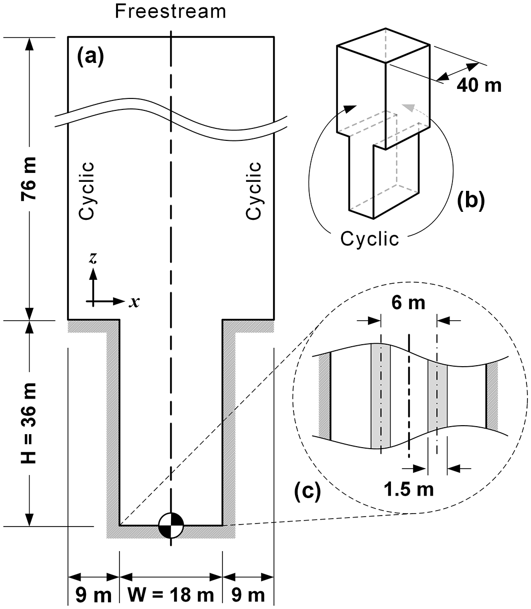
Figure 1Schematic of the solution domain representing the infinite street canyon geometry from Zhong et al. (2015): (a) basic dimensions and locations of cyclic and freestream boundaries, (b) isometric view of the domain showing lateral dimension and corresponding cyclic boundaries, and (c) top view of ground surface indicating size and position of simulated traffic lanes.
As illustrated in Fig. 1, the solution domain representing an infinite deep street canyon will be used for this study throughout. To facilitate discussion, x will be referred to as the spanwise direction, y the lengthwise direction, and z the vertical direction. The origin of the domain is located on the street level, at the intersection between the spanwise (x−z) and lengthwise (y−z) planes of symmetry. The span of the street section (W) is 18 m, and the building height (H) is 36 m, resulting in an height-to-span aspect ratio of two. The freestream boundary is located at 76 m above the canyon roof, or 112 m above street level, from which meteorological conditions are specified. The canyon roof extends 9 m on each side of the spanwise direction, as shown in Fig. 1a. The street section length is set to 40 m, as shown in Fig. 1b, centered about the domain origin. Traffic emissions are introduced as two 1.5 m wide sections in equidistant arrangement, as shown in Fig. 1c, and are assumed to be continuous and spatially uniform along both sections. Cyclic conditions are imposed on the spanwise and lengthwise boundary pairs to ascertain periodicity in the corresponding directions, as well as to allow turbulent flow structures to freely develop across the solution domain. To prevent accumulation of pollutants through the spanwise cyclic boundaries while maintaining background concentrations, chemical species will be introduced from the upstream spanwise boundary at specific, spatially uniform mixing ratios, while a zero gradient boundary condition will be imposed on the downstream spanwise boundary, allowing excess pollutants to leave the solution domain.
Initially, the dynamics of this model framework will be evaluated using the stationary laser Doppler anemometry (LDA) measurements of Li et al. (2008). This is followed by a transient simulation run with reaction kinetics activated. Boundary conditions representative of a working day in Berlin in July 2014 will be used. Diurnal variations for ambient wind and thermodynamics are extracted on an hourly basis from the regional model results of Kuik et al. (2018) using the Weather Research and Forecasting (WRF) Model (Skamarock et al., 2008). Meanwhile, hourly traffic emissions are derived from speciated spatiotemporal redistribution of annual NOx emission levels provided by the Berlin City Senate. Urban background concentrations for NO, NO2, and O3 are obtained from the Berlin Air Quality Measurement Network (Berliner Luftgüte-Messnetz, BLUME). In-canyon vertical and horizontal profiles will be compared against corresponding stationary model runs at specific times of the day, in addition to diurnal variations of species concentration at specific locations.
2.1 Prognostic equations
The prognostic equations employed in the present model will be formulated using a weakly compressible framework. This generalizes the theoretical foundation and opens up possibilities of direct coupling with other compressible regional models such as WRF in the future. These equations form the dynamic core of the modeling framework, to which the conservation equations for mass, momentum, energy, and species are to be solved numerically to determine the spatial and temporal distribution and evolution of the prognostic variables, namely, wind velocity components (ui), pressure (p), internal energy (e), and mass mixing ratios for each gas-phase component species (yq):
where the notation represents the substantial derivative, ρ is the density of the gas mixture, is the mixture enthalpy, and r is the net chemical production rate of each gas-phase species. The Coriolis coefficient is denoted by 2sin (ϕ)ωj, as a function of the planetary angular velocity ω, and the latitude of the point of interest ϕ. The shear stress tensor τij in Eq. (2) is represented by , where μ is the dynamic viscosity, and δij is the Kronecker delta. Enthalpy changes from chemical reactions are deemed negligible and thus are not considered in Eq. (3).
Due to the computational effort required to directly resolve all possible turbulent scales in any flow of practical interest, some form of statistical treatment must be adopted. In the LES model approach, this is realized by decomposing the instantaneous scalar variable φ into a resolved scale, 〈φ〉, and a residual scale, φΔ, through spatial convolution with a low-pass filter kernel F (Leonard, 1974):
The filter width Δ is associated with the smallest turbulent scale that can be retained in the resolved scale. In practice, Δ is derived from the local mesh dimensions, for example, the cube root of the cell volume, such that . Thus all turbulent scales residing within the resolved scale, i.e., those with spatial scales larger than the attenuation threshold defined by F(Δ), can be captured directly with the computational grid, while the residual turbulent scales, which are commonly referred to as the subgrid scale (SGS), are modeled.
As with Reynolds averaging for time-averaged scalars, additional terms will result from the filtering operation of Eqs. (1)–(4), deriving from the advective term in the substantial derivative Dt〈φ〉:
which implies
where is known as the SGS term, and in the case of the momentum Eq. (2) this is referred to as the SGS stress tensor and is denoted simply as σij. Further, in a compressible flow framework, where density also varies, additional SGS terms from density filtering will be introduced in Eq. (1). This can be avoided, however, by performing the filtering operation on a density averaged scalar, where through a process known as Favre filtering (Favre, 1965). The corresponding filtered transport equations for Eqs. (1)–(4) then become
where the notation for Favre-filtered substatial derivative is written as . In addition, Vreman et al. (1995) show that nonlinearities arising from filtering of diffusion terms can be neglected for weakly compressible flows based on a priori direct numerical simulation (DNS) data. The expanded form for the corresponding SGS terms for Eqs. (7)–(10) are presented below:
Detailed discussions pertaining to the modeling and parameterization of the remaining SGS terms described in Eqs. (12)–(14) can be found in Martín et al. (2000).
Numerous approaches are available for modeling the SGS terms (Garnier et al., 2009). A common method, first proposed by Smagorinsky (1963), is to model the SGS stresses by invoking the gradient transport theorem:
where . The closure of subgrid scale viscosity μΔ is, in turn, achieved by using representative turbulent scales. Based on the one equation model of Deardorff (1980) for incompressible flows, Yoshizawa (1986) proposed a similar closure scheme for weakly compressible flows using :
and the subgrid scale viscosity μΔ can then be evaluated as follows:
in which both Ck and Cϵ are dimensionless single-valued constants set to 0.094 and 1.05, respectively.
2.2 Thermophysical and chemistry models
In the current study, the photostationary NO–NO2–O3 mechanism (Leighton, 1961) will be considered. The mechanism comprises the photodissociation of NO2 into NO, the titration of O3 by NO to form NO2, and an intermediate third-body reaction for in situ ozone production through oxygen radicals originated from NO2 photolysis:
Reaction (R1) describes the photodissociation of NO2, whose rate constant k is calculated as a function of the solar zenith angle (χ):
Meanwhile, the rate constants for Reactions (R2) and (R3) are based on the Arrhenius rate law:
where A and TA are the corresponding pre-exponential factor and activation temperature for each reaction. All parameters for the aforementioned reactions are tabulated with reference in Table 1.
Saunders et al. (2003)Huie et al. (1972)Burkholder et al. (2015)Table 1Reaction rate parameters for the photostationary NO-NO2-O3 mechanism. Units are kmol, m3, s, and K.
In the current study, air is modeled as a mixture of its primary constituents, namely N2 and O2, but the effects of H2O and CO2 are not considered at this stage. Together with the additional gaseous species introduced in Reactions (R1) to (R3), i.e., NO, NO2, O(3P), and O3, Eq. (14) consists of six species transport equations that need be solved. The individual species net production rate rq in Eq. (14) is determined by summing up the generation and consumption rates of the corresponding species across all relevant reactions. As non-limiting examples, the net production rates for NO, NO2, and O3 for the current chemical mechanism are calculated as follows:
Transport and thermophysical properties for these species are available from McBride et al. (1993). Temperature dependence of specific heat for species q at constant pressure () is presented as a polynomial function:
where the polynomial coefficients ai are obtained using a least-squares fit and Rq is the specific gas constant for the species of interest. Meanwhile, dynamic viscosity (μ) is represented using Sutherland's law:
where AS (in Pa s K−1) and TS (in K) are species-specific single-valued coefficients. The thermodynamic state of the mixture is determined by the ideal gas relation:
where R is the specific gas constant for the gas mixture.
2.3 Model implementation
The open-source finite-volume computational continuum mechanics framework
OpenFOAM (Weller et al., 1998) has been used as the modeling foundation for this
work, due to its ability to handle compressible reactive flows
in an unstructured grid arrangement. More specifically, the current
flow solver and related data processing utilities are derived from OpenFOAM
version 7, maintained by CFD Direct Ltd. All pertinent modifications
and augmentations at the source level are performed in the C++
programming language. The OpenFOAM framework contains core classes for
LES and gas-phase thermophysics, chemistry, and reaction kinetics.
To adopt OpenFOAM for urban-scale chemical transport modeling,
a custom solver, urbanChemFoam, derived from the existing
rhoReactingFoam, has been developed to enable geodetic and
solar calculations using a Julian-Day-based date and time module.
The solar state, represented by the solar zenith angle (χ) can
either be calculated at each time step using the algorithm of
Meeus (1998), via a user-defined reference time and location, or
set to a fixed value by the user throughout the model run.
Additional components have also been developed to operate in conjunction
with urbanChemFoam. As existing chemical reactions in OpenFOAM
are functions only of the thermodynamic state, a new reaction class,
called irreversiblephotolysisReaction, has been developed to
model photodissociation as a function of the cosine of the solar
zenith angle. Further, surface emissions, for instance from traffic
sources, are provided in units of mass flux (i.e., kg s−1).
These are typically introduced in chemical transport models as
volumetric source terms in the interior cell nodes of the corresponding
surface boundaries. On the other hand, in OpenFOAM, emissions must be
expressed in terms of fluxes of mass mixing ratios (in kg s−1
per kilogram of mixture). Since the mass of the mixture, and therefore the
corresponding mixing ratio flux, is not known at the boundary surface,
this necessitates the implementation of a new boundary condition,
simpleEmission, in which the mixture mass at the boundary is
calculated using the adjacent interior cells, allowing surface emissions
to be prescribed as mass flux boundaries. To prevent spurious accumulation
of pollutant species through the spanwise cyclic boundaries,
the default cyclic boundary patches in OpenFOAM have been
augmented to behave as a Neumann boundary condition (zeroGradient)
on the downstream boundary of the flow, while maintaining background
concentrations on the upstream boundary, similar to a Dirichlet boundary
condition (fixedValue). These modified boundary patches are
referred to as cyclicZeroGradient and cyclicFixedValue,
respectively. Finally, a preprocessing utility, initCanyon,
has been developed to provide an initial velocity perturbation in the
solution domain, allowing turbulence flow structures to freely develop
between the spanwise and lengthwise cyclic boundaries.
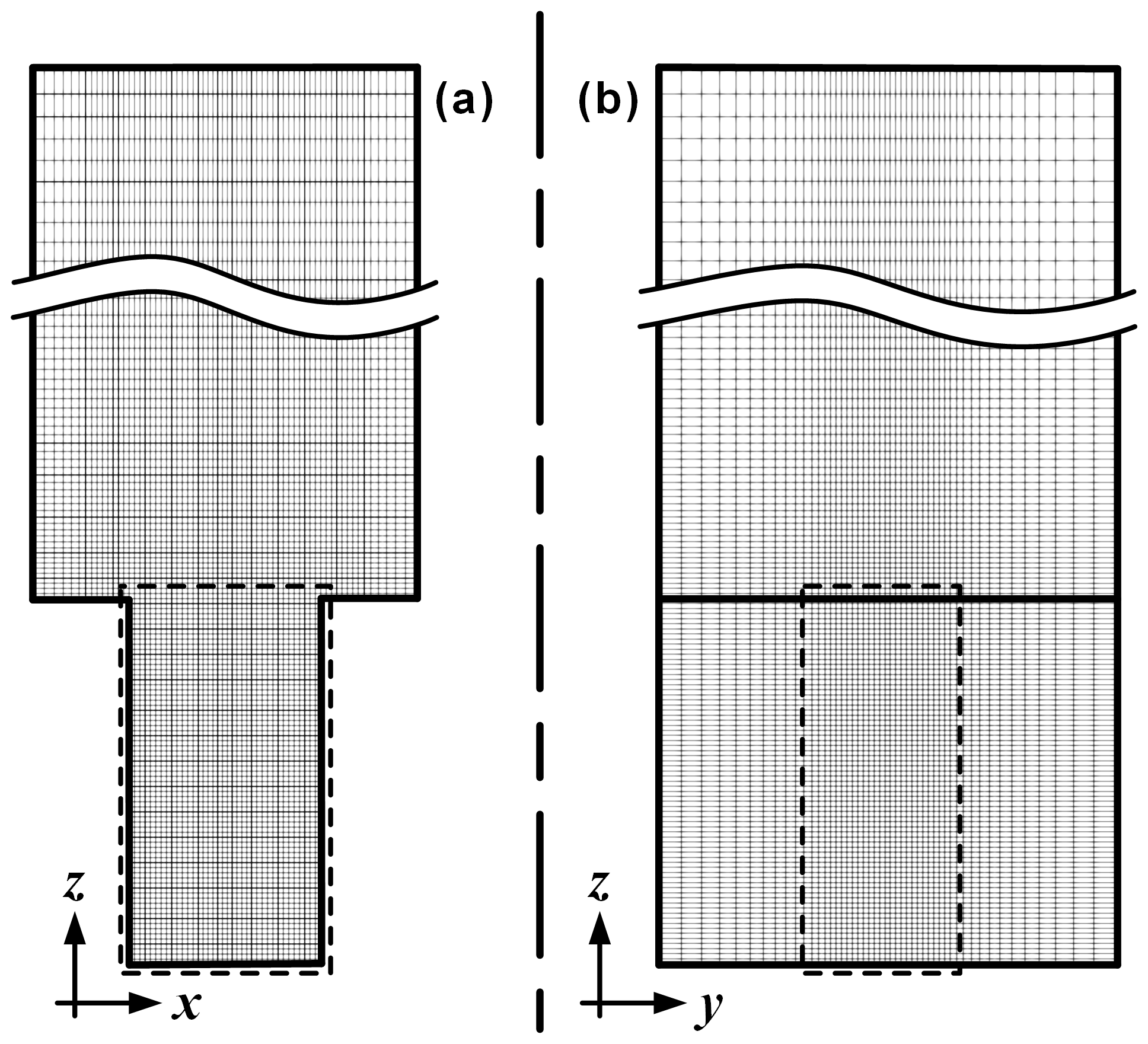
Figure 2Grid distribution of the canyon geometry in the (a) x−z plane and (b) y−z plane. Cell size in the canyon core region (dashed line) is m3.
2.4 Domain discretization and decomposition
The solution domain is discretized using the OpenFOAM blockMesh
utility, which generates a conformal hexahedral grid.
A core region is defined by a 9 m lengthwise section
about the domain origin, covering the entire span and height of
the street canyon, where grid cells are uniform and have an aspect ratio near unity. Grid cell grading is introduced beyond the core region
so that cell size gradually expands at a rate according to a
user-specified final expansion ratio relative to the core cell size,
which dictates the size of the furthermost cells.
For the present study, this expansion ratio is set to 1:2 in the
spanwise direction, 1:3.2 in the lengthwise directionm and 1:4 in the heightwise
direction. Two mesh configurations of core cell sizes
of 1 m (coarse mesh) and 0.5 m (fine mesh) have been
deployed in the evaluation study, corresponding to a total cell count of
43 500 and 344 000 cells. Following the results from the stationary
evaluation (Sect. 3), the transient study is conducted
only at the fine mesh level. Figure 2 shows the mesh cell
distribution for the fine mesh arrangement (core cell size 0.5 m),
showing core and graded regions.
The numerical schemes used in the discretization of the prognostic equations are second-order accurate in time and space. A colocated grid approach is used, in which pressure–momentum coupling is achieved using a fourth-order interpolation scheme (Rhie and Chow, 1983). For each time step, each discretized prognostic equation is solved iteratively using the biconjugate gradient method (van der Vorst, 1992) with a diagonal incomplete lower–upper matrix factorization (ILU) preconditioner, until the global normalized residual falls below a specified convergence criterion, in this case 10−5. Mass conservation is enforced at every iteration by solving an iterative pressure correction equation until the aforementioned residual threshold is reached. Typically, the pressure correction equation converges in two to three iterations and about five to eight iterations for the prognostic equations at each time step for the sizes of grid cells and time step considered in this study. Grid decomposition for parallel computing is performed in three dimensions using a dual recursive bipartitioning algorithm (Chevalier and Pellegrini, 2008).
For the purpose of evaluating the LES street canyon model, a stationary run is performed for which LDA flow measurement data are available from Li et al. (2008) for a scale model infinite canyon arrangement, also with a height-to-width aspect ratio of two, conducted in a water tunnel. The horizontal velocity of this simulation is prescribed at the freestream boundary, denoted as U∞. An initially quiescent velocity field is imposed in the canyon region, while a linear spanwise flow profile – i.e., , where z is the elevation above the canyon and z∞ and U∞ are the elevation and velocity at the domain freestream boundary, respectively – is assigned above the canyon. A value of 3.52 m s−1 has been used for the spanwise velocity at the freestream boundary. Turbulence in the flow domain is initiated using a superposition of randomized velocity perturbation, with a magnitude of up to 10 % of the freestream velocity, into the initial flow field. Simulations are conducted using the coarse (1 m) and fine (0.5 m) mesh configurations, both at a uniform time step of 0.01 s. Each simulation is given a 6 h (21 600 s) spin-up period before sampling begins for a period of 3600 s at a frequency of 100 Hz, from which turbulent statistics are constructed.
To coincide with the LDA measurements, sampling points for the LES simulations are located along vertical stations at , 0, and +0.25, denoting upstream, central, and downstream positions with respect to the direction of freestream flow, at the lateral plane of symmetry (y=0). The time-averaged velocity components and subgrid scale turbulent kinetic energy (SGS TKE) at each sampling point are calculated as the arithmetic mean of the respective time series. The turbulent velocity fluctuation in each direction is, in turn, determined using the L2 norm of the central difference of the instantaneous velocity components. The resolved scale TKE can then be calculated using its definition . Note that the LDA mean and fluctuation measurements represent a Reynolds average of the flow field, while the LES model data in the present study attempt to duplicate these results using only data contained in the resolved scale.
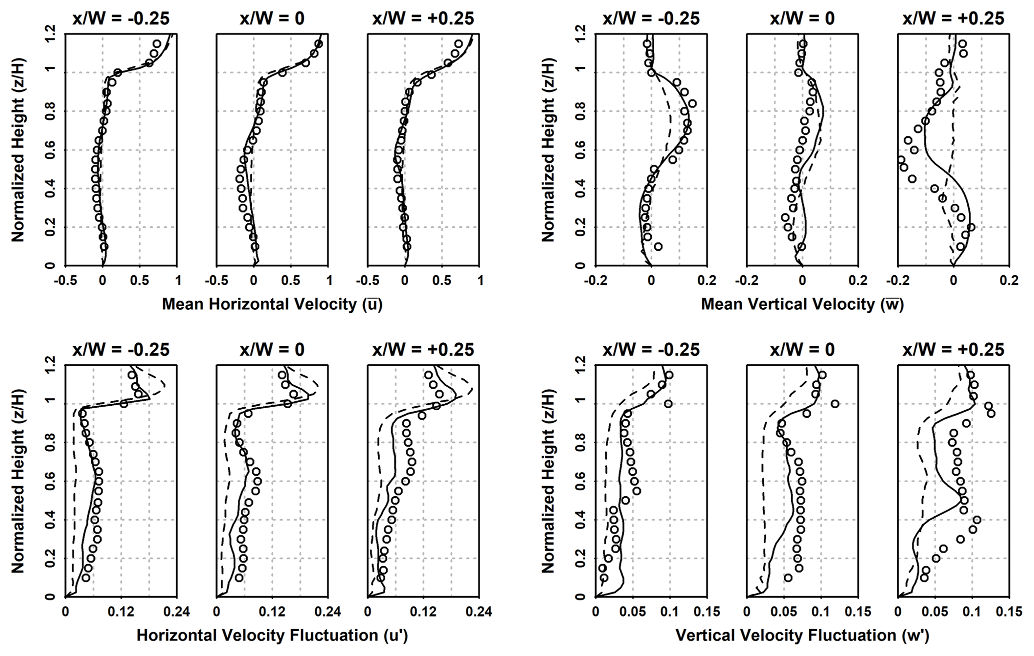
Figure 3Normalized vertical profiles of the of resolved mean horizontal (top left) and vertical (top right) velocity components, as well as horizontal (bottom left) and vertical (bottom right) velocity fluctuations, for stations located at (left), 0 (middle), and +0.5 (right) in the idealized street canyon geometry. Solid lines indicate the present study using fine mesh; dashed lines indicate the present study using coarse mesh; and symbols represent the LDA measurements from Li et al. (2008).
Figure 3 shows the comparison between the present LES results on both mesh arrangements with the LDA measurements at the aforementioned vertical stations. In this figure, both the fine and coarse mesh results are in excellent agreement with respect to horizontal time-averaged velocity (, upper-left panel), with the exception of a slight overprediction above the canyon at . For the time-averaged vertical velocity component (, upper-right panel), the fine mesh solution is able to adequately capture the profiles. There is a discrepancy at , but the salient features are still well represented. In comparison, the coarse mesh results underpredict the velocity magnitude. In light of the fine mesh results, this observation indicates an issue with grid convergence. In addition, substantially better agreement in turbulent fluctuation (u′ and w′, lower-left and lower-right panels, respectively) can be found with the fine mesh results. There are still minor differences between the fine grid LES results and the LDA measurements, but they can be attributed to the use of only resolved turbulent fluctuations in deriving the time-averaged results. In addition, as Zhong et al. (2015) also indicated, the circumstances under which the experiment (Li et al., 2008) is conducted, methods of vortex generation, for instance, are not modeled, which could attribute, at least in part, to the observed differences.
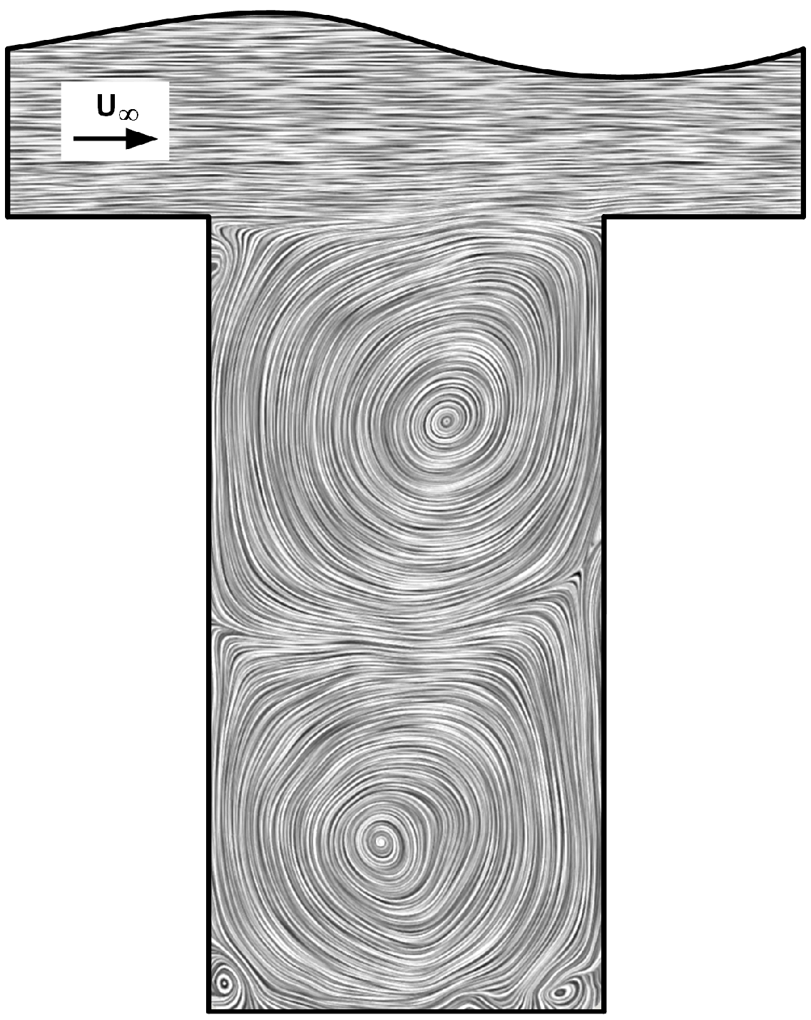
Figure 4Line integral convolution representation of the velocity vector along the x−z plane. Inset indicates direction of freestream flow.
The mean flow field in the canyon along the lateral plane of symmetry has been obtained by averaging the instantaneous velocity field at interval of 300 s for over the 3600 s sampling period for the fine mesh configuration. It is presented in Fig. 4 using a line integral convolution representation (LIC; Cabral and Leedom, 1993). It depicts a typical skimming flow regime occurring in idealized urban canyon arrays (Oke, 1988), where a free shear layer develops over the canyon at resulting from turbulent interaction between the building roof and the freestream flow upstream. Two vertically stacked primary recirculation zones exist inside the canyon, in line with existing works on deep street canyons (Baik and Kim, 1998; Li et al., 2008). However, additional, minor vortices are also observed at the corners at the street level, which may lead to additional isolation of street-level emissions, for instance, from traffic sources.
Although there is little mass transfer between the bulk flow and the canyon in the skimming flow regime, as indicated by the RANS vertical velocity component () near the canyon roof in Fig. 3. Based on the mean flow structures indicated in Fig. 4, weak vertical interaction still exists downstream in the canyon between the primary recirculation zones. It can be seen that pollutants from the street level can be carried upwards by the bulk flow, first through the lower recirculation zone in an counterclockwise direction downstream. Further exchange then takes place between the lower and upper recirculation zones, eventually reaching the canyon roof clockwise around the upper recirculation zone, where it merges with the bulk flow, again downstream in the canyon.
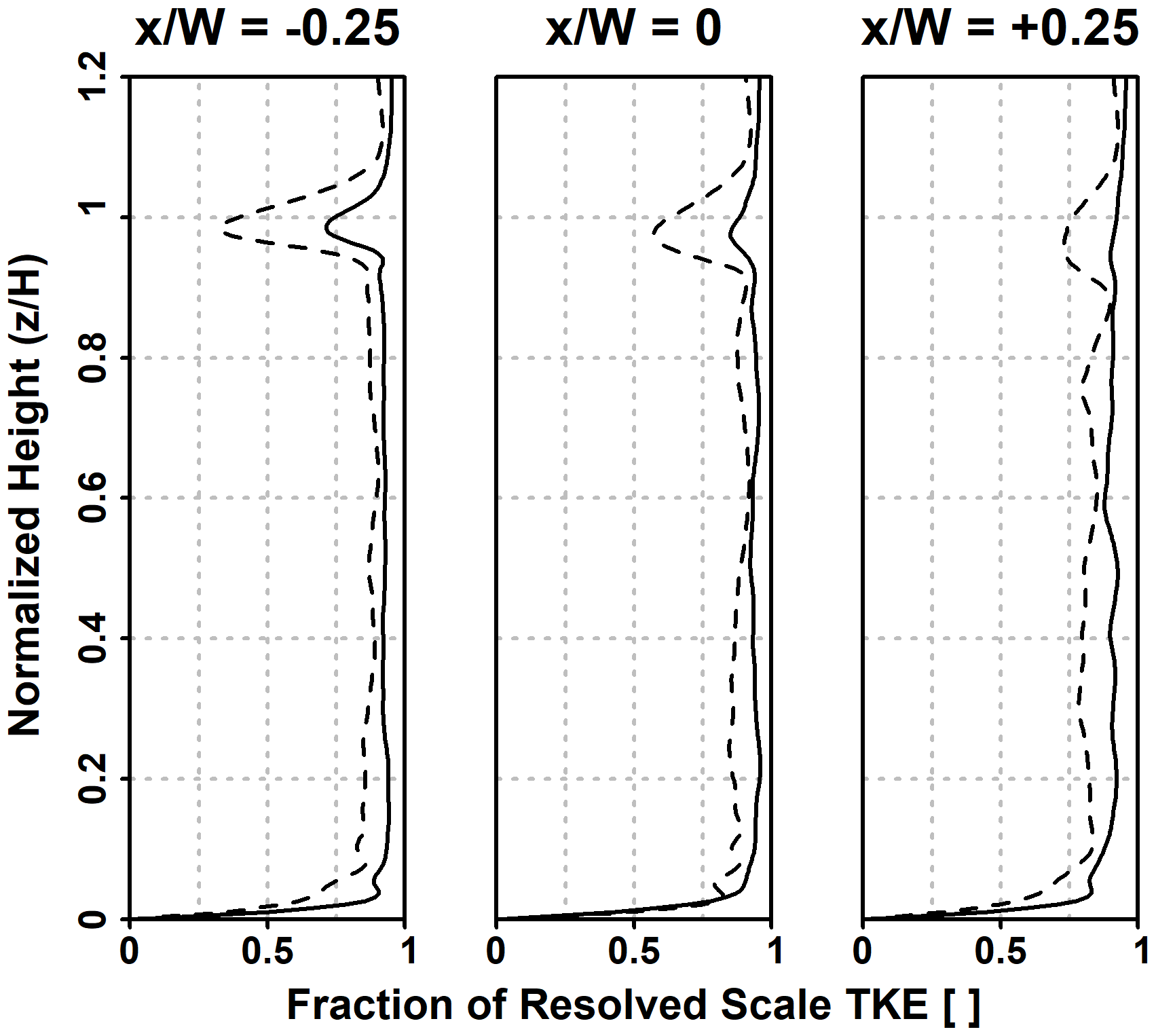
Figure 5Fraction of resolved scale TKE of total (resolved and SGS) TKE for the three stations in the street canyon. Solid lines indicate fine mesh, and dashed lines indicate coarse mesh.
To further evaluate the resolution of turbulent scales under each mesh configuration, the fraction of TKE as its simulated total – i.e., the sum of resolved and SGS TKE – is calculated along the three vertical stations, as presented in Fig. 5. The free shear layer on top of the canyon roof region is accompanied by a sudden increase in turbulence kinetic energy upstream in the canyon core, which dissipates downstream (Driver and Seegmiller, 1985). However, a decrease in resolved scale TKE fraction can be observed in this region. In particular, the attenuation in turbulence resolution is significantly higher in the coarse mesh than in the fine mesh configuration, with a minimum of 36.0 % and 73.6 % for the respective mesh density. This indicates a diminished capability of the coarse mesh to adequately capture turbulent structures explicitly, which contributes to the discrepancies in the vertical profiles observed in Fig. 3. Nevertheless, the resolved TKE fraction in the canyon core and the bulk flow regions (that is, outside of the free shear flow region) remains very high for both grid configurations. Based on a 95 % confidence interval for regions away from walls and the free shear layer, the resolved fraction is calculated to be 86.0 %–87.5 % for the coarse mesh and 92.6 %–93.3 % for the fine mesh. This suggests that the turbulent resolution in the free shear region could be summarily resolved by local mesh refinement. However, based on Fig. 5, the fine mesh configuration provides an adequate resolution of turbulent flow structures. Hence, subsequent discussions will be made exclusively with the 0.5 m mesh configuration.
The transient study consists of two sets of model runs. The first model set is a fully transient run, where boundary conditions are prescribed using the diurnal profiles for meteorological conditions, solar state, background concentrations, and traffic emissions. For the second set, a series of stationary runs are conducted with boundary conditions fixed at 08:00, 12:00, 16:00, and 20:00 UTC. Each run begins 6 h prior to the start of the data sampling period and is conducted using the fine mesh arrangement (core cell size 0.5 m) and a constant time step of 0.05 s. Vertical profile data are extracted at , 0 and +0.25, and in-canyon horizontal profile data are extracted at z=2 m and and 0.75.
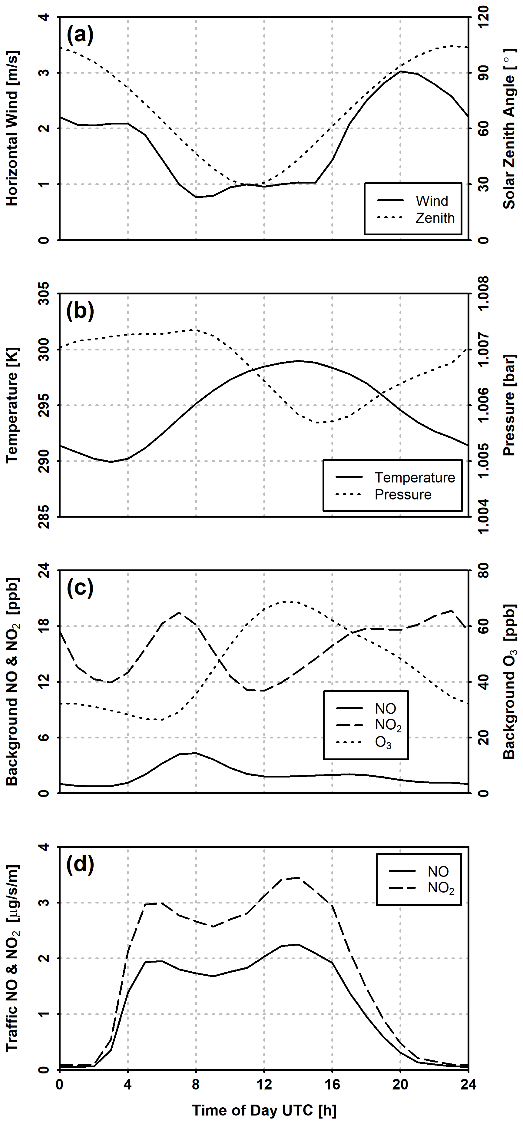
Figure 6Prescribed conditions for the transient simulation: (a) horizontal freestream wind velocity and solar zenith angle; (b) ambient temperature and density; (c) urban background NO, NO2, and O3 concentrations; and (d) workday traffic NO and NO2 emissions per unit street section length.
4.1 Model configuration
Figure 6 shows the diurnal profiles for meteorology, background concentrations, traffic emissions, and solar state applied to the transient model run, representative of a typical work day for the city of Berlin in July 2014. The freestream horizontal (u) wind, as well as the solar zenith angle (χ), is presented in Fig. 6a, while the air temperature and pressure are illustrated in Fig. 6b. The profiles for wind, pressure, and temperature have been obtained from the hourly WRF model output of Kuik et al. (2018) by first interpolating the pressure coordinates to the freestream height (112 m) of the canyon and averaging them at each hour across every day in the period of July 2014. A neutral boundary layer is assumed in order to suppress lengthwise convective cells formed under thermal stratification, which introduces grid dependence in the numerical solution in a cyclic finite-length street canyon (Davies-Jones, 1970). The solar zenith angle is calculated on line at each time step. Sunrise and sunset are defined when the solar zenith angle reaches the 90∘ crossing. For the 24 h simulation period, sunrise occurs at 02:55:06.83 UTC, and sunset takes place at 19:25:26.13 UTC. In the mean time, the solar zenith angle reaches a minimum of 29.42∘ at 11:10:24.67 UTC.
The profiles for background concentrations of NO, NO2, and O3, shown in Fig. 6c, are obtained from hourly averages on all full working days (Tuesdays and Wednesdays; Mondays and Thursdays have been excluded to minimize end-effects carried over from adjacent non-working days) from observation data of urban background stations located on Amrumer Straße (DEBE010) and Nansenstraße (DEBE034) in Berlin. Days with missing measurement data are discarded entirely, leaving 17 d with intact hourly measurements. The traffic NO and NO2 emissions, as presented in Fig. 6d, are estimated from annual NOx aggregate for the city of Berlin in 2014 using hourly traffic data and vehicle fleet composition provided by the Berlin City Senate. Temporal redistributions of annual traffic emissions are inferred by traffic density for major street segments, from which a representative flow speed and level of service are determined. Emission factors for NOx can then be calculated assuming a standard fleet composition for the street segment of interest. The NOx emission is then partitioned into NO and NO2 according to the Gridding Nomenclature for Reporting (GNFR) for the road transport source sector categories (Cranier et al., 2019), with a molar fraction of 0.95 for NO and 0.05 for NO2 for gasoline exhaust (F1) and 0.7 (NO) and 0.3 (NO2) for diesel exhaust (F2).
All runs are conducted with four cluster nodes, each comprising two Intel Xeon Platinum 9242 processors and 384 Gb of physical memory. Based on OpenFOAM run statistics, each simulation hour of model run requires on average 8623±148 s in processor time or 8788±145 s in wall clock time to complete, with a 95 % confidence interval over all transient and stationary runs. All output data are written to file every 30 s of simulation time, and corresponding hourly means are calculated at the top of each hour using a central window average spanning 3600 s.
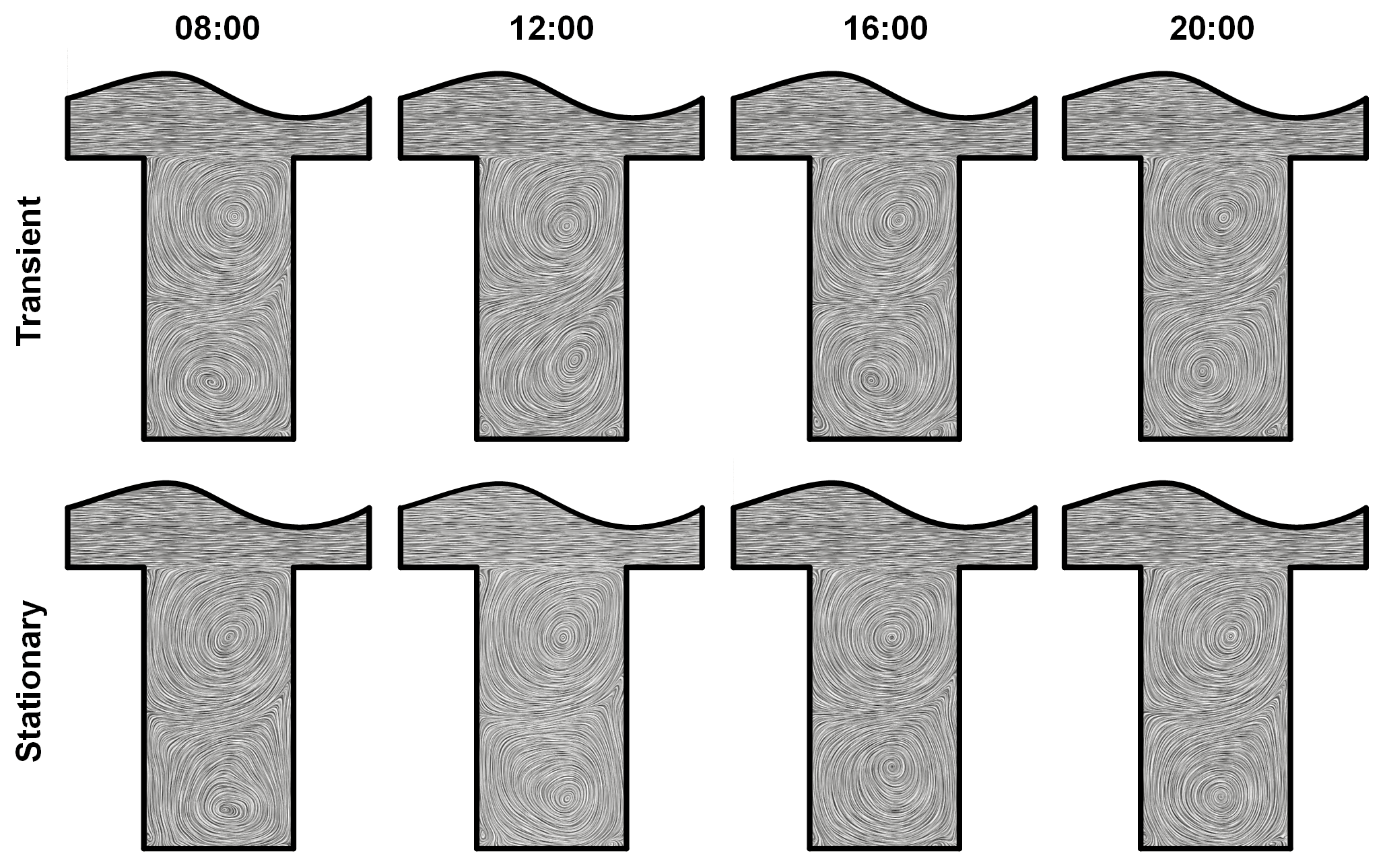
Figure 7Comparison of LIC representation of hourly mean velocity vector along the x−z plane for transient (top) and stationary (bottom) model runs at various points of time in UTC.
4.2 Results and discussion
Figure 7 shows the qualitative comparison based on the LIC representation of the hourly average velocity field between the fully transient run and the stationary runs at each specific time. As with Fig. 4, two vertically stacked primarily recirculation regions are visible in all cases, as well as secondary vortices located at the street-level corners. Differences in fluid motions can be observed between the transient and stationary model runs at the same time, as indicated by the relative displacement in the primary vortex locations. This is a result of the differences in temporal variations in the meteorological conditions, which are held constant at specific times in the stationary runs, as indicated in the difference in hourly vertical profile of horizontal velocity component in the freestream region () between the transient and stationary runs, as shown in Fig. 8. The momentum exchange in and out of the canyon is restricted by the shear region, defined by a strong mean shear () at the canyon roof (). The in-canyon () velocity component profiles follow a general feature proportional to the magnitude of the freestream velocity. Nevertheless, while the diurnal variation in freestream velocity is approximately 2 m s−1, as illustrated in Fig. 6a, the corresponding change in the in-canyon velocity magnitude is in only in the order of a few centimeters.
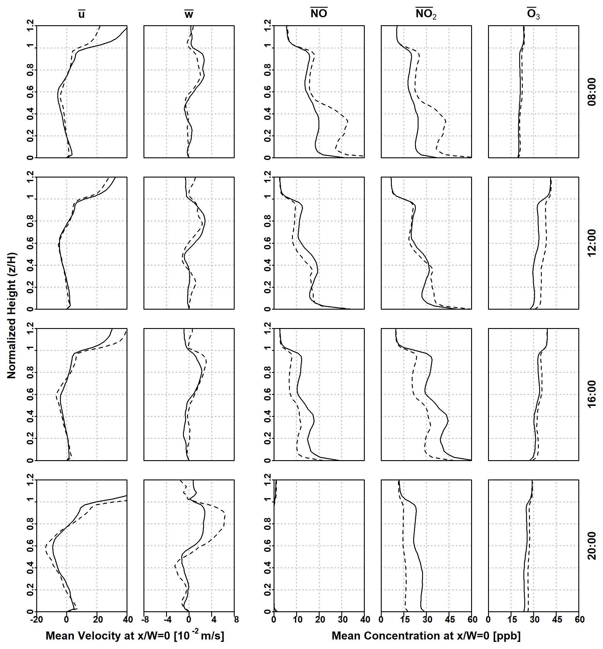
Figure 8Comparison of vertical station profiles of mean velocity components and species concentrations for transient and stationary model runs at various points of time in UTC. Solid lines indicate transient runs, and dashed lines indicate stationary runs.
However, deviations of up to about 20 ppb in pollutant concentrations can be observed in the vertical profiles in Fig. 8, even though the rate of hourly traffic NO and NO2 emissions are identical for the indicated times between transient and stationary simulations. The discrepancy is particularly large at 08:00 and 20:00 UTC, This is due to a two factors contributing to the difference between the two types of model runs. First, in addition to meteorological conditions, the rates of reactions, background concentrations, and emissions are also held constant in stationary simulations, while the transient run follows a diurnal variation, which results in a difference in equilibrium composition in the street canyon and freestream regions. This also brings about the second factor; i.e., the difference in boundary conditions also leads to a difference in cumulative pollutant concentration at the beginning of the sampling period.
Two observations can be made from this comparison. First, to the extent of the meteorological conditions considered in this study, there is little change in the in-canyon flow field between stationary and non-stationary runs. This is not surprising, considering that the shear layer in the roof region attenuates the dynamics inside the canyon from those above the buildings. Accordingly, the in-canyon wind should be less sensitive to the temporal variations in the freestream flow. On the other hand, significant changes can be observed in pollutant concentrations under stationary and non-stationary treatment. As such, temporal variations in emissions and background conditions, which are not considered in stationary runs, are significant and cannot be neglected. In light of the above observations, where wind and flow distributions are of primary concern, stationary model runs would likely suffice. However, if the focus of the study is on pollutant transport and transformation, temporal variations of background concentrations and emissions will have an appreciable influence on the model concentrations, and thus a non-stationary approach should be considered.
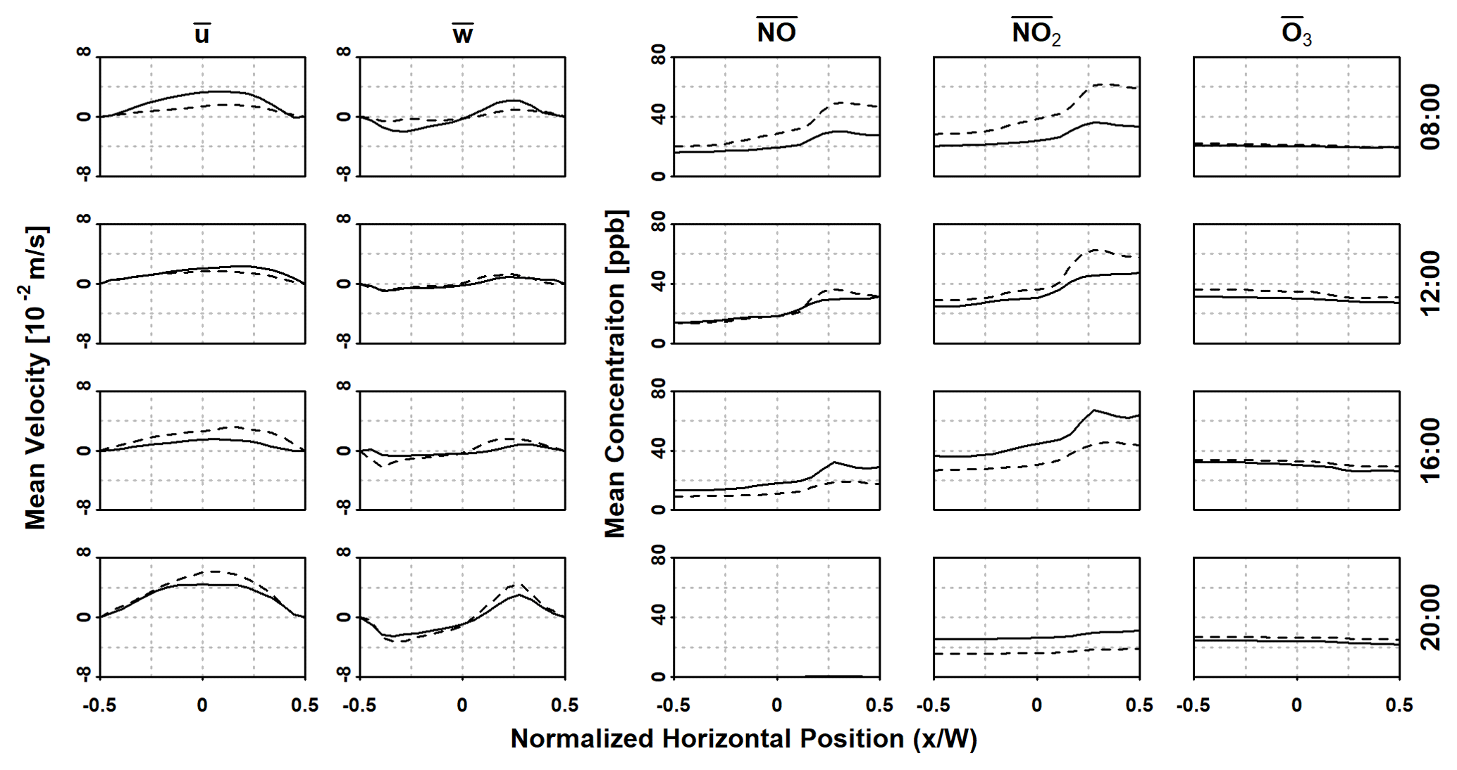
Figure 9Comparison of horizontal station profiles of mean velocity components and species concentrations at an elevation of 2 m for transient and stationary model runs at various points of time in UTC. Solid lines indicate transient runs, and dashed lines indicate stationary runs.
A cascade of concentrations for all species considered can be identified, corresponding to the individual primary vortices seen in Fig. 4, concurring with the numerical results of Bright et al. (2011) for a street canyon of unity aspect ratio. The concentrations of NO and NO2 generally increase along each level of cascade (and hence each primary vortex), due to the higher flow velocity in the outer regions of each vortex, causing pollutants to be transported first to the top of the vortex. A portion of NO and NO2 is then transferred at the top of the lower vortex into the bottom of the upper vortex through shear motion. The bulk motion in the upper vortex leads to an increase in vertical concentrations along the vortex, albeit in lower concentrations, before leaving the canyon through the shear layer at the roof level.
In addition, there is a reciprocal relationship between the concentrations of NO and NO2, as well as O3. This is expected as the O3 originates from the freestream and is titrated through Reaction (R3) by the NO originating from street-level traffic. However, the concentration of in-canyon O3 is not substantially different from freestream levels, at least in comparison with the NO and NO2 levels. This is, in part, due to the in situ production of O3 through photodissociation in Reaction (R1). The exception is 20:00 UTC, where the hourly sampling and averaging takes place with the absence of the photolysis Reaction (R1), as the solar zenith angle (χ) reaches 90∘ at 19:25 UTC, leaving the titration Reaction (R3) the only active reaction in the mechanism. Combined with a low traffic emission, as indicated in Fig. 6d, this leads to a moderate decrease in O3 while depleting the NO in the canyon.
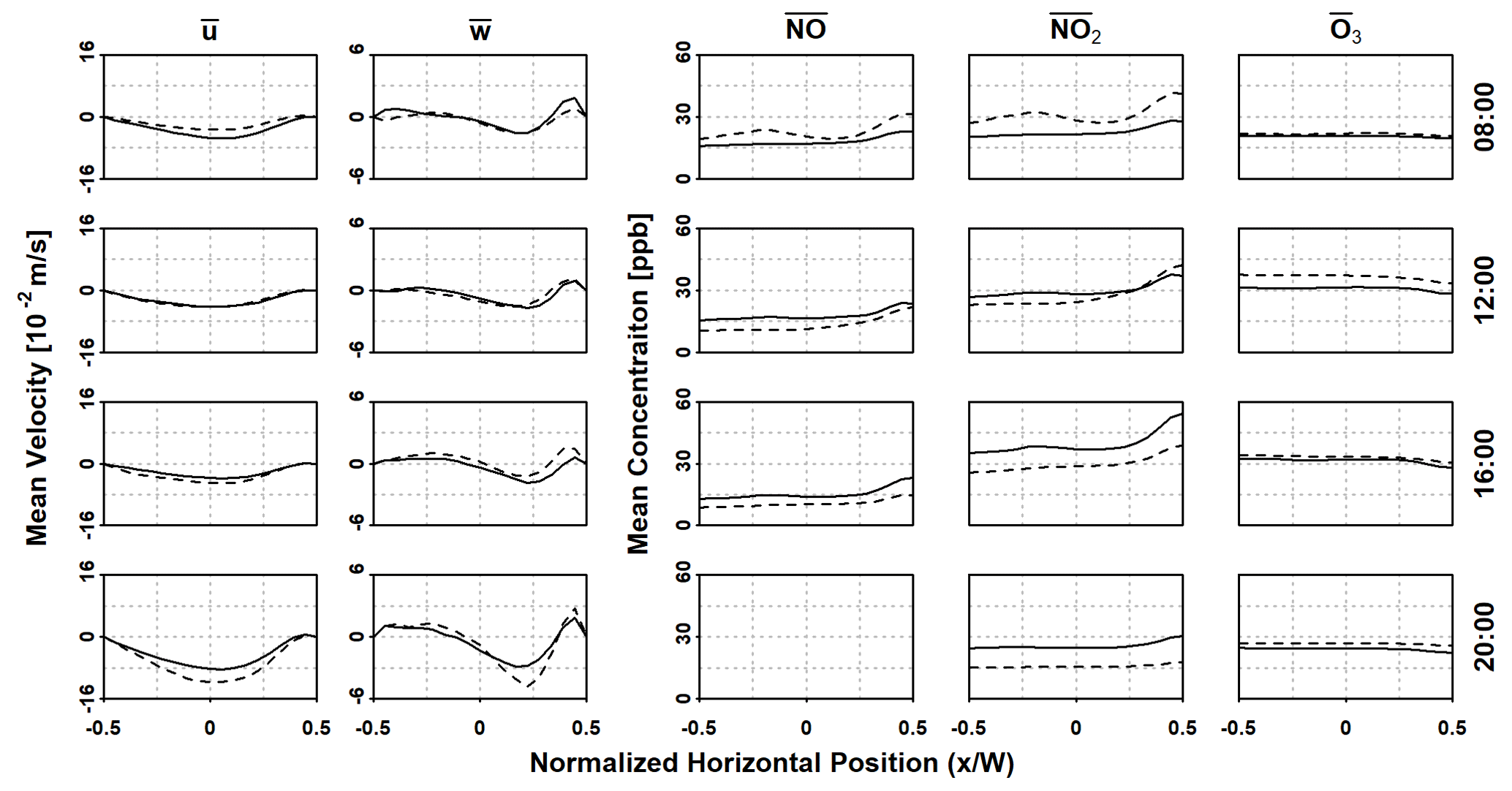
Figure 10Comparison of horizontal station profiles of mean velocity components and species concentrations at a normalized elevation of for transient and stationary model runs at various points of time in UTC. Solid lines indicate transient runs, and dashed lines indicate stationary runs.
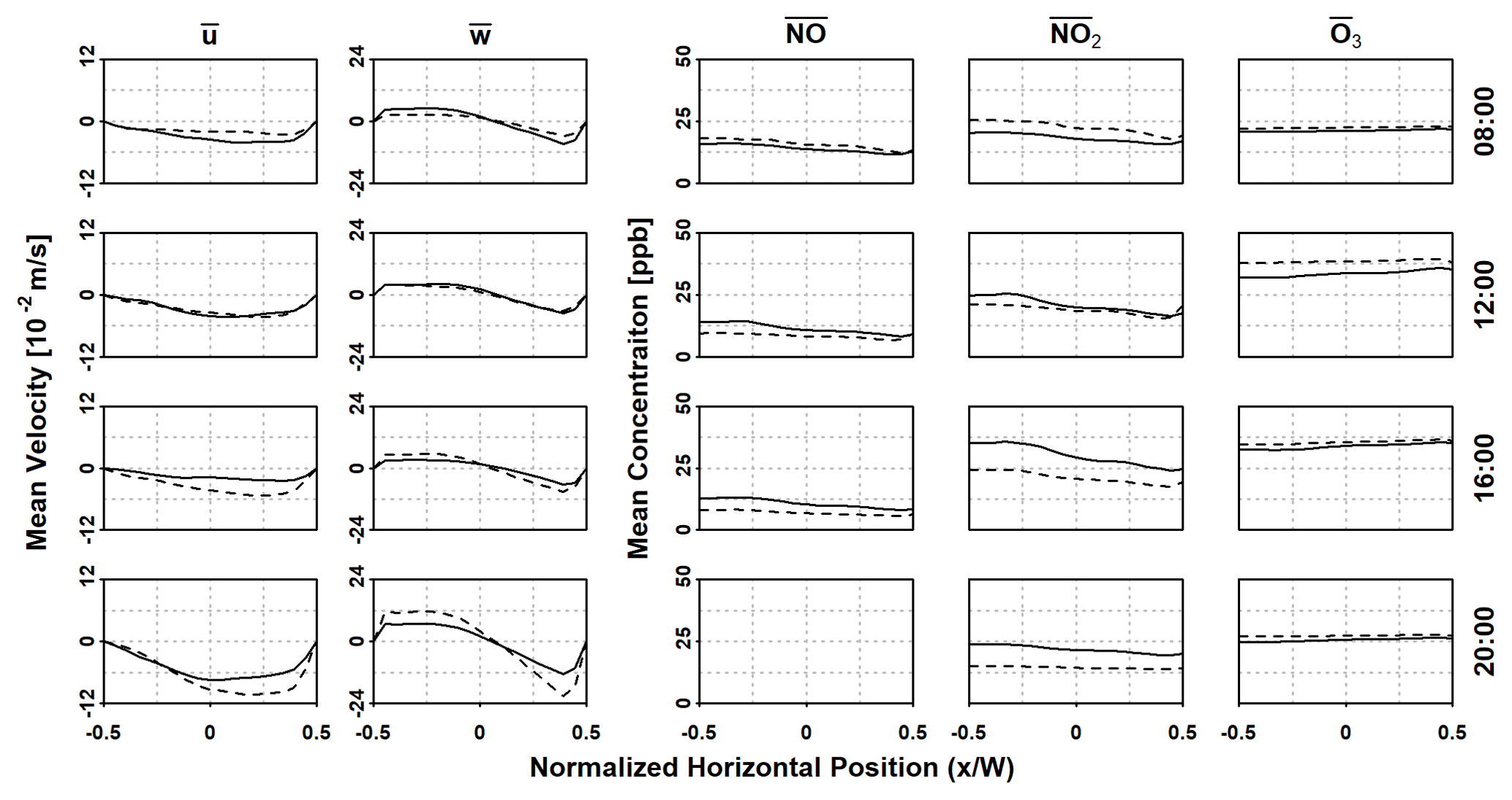
Figure 11Comparison of horizontal station profiles of mean velocity components and species concentrations at a normalized elevation of for transient and stationary model runs at various points of time in UTC. Solid lines indicate transient runs, and dashed lines indicate stationary runs.
Horizontal profiles of velocity and concentrations are presented in Figs. 9, 10, and 11, evaluated at 2 m, 18 m (), and 27 m () above the canyon street level respectively, representing street level, between the two vertical primary vortices, and the upper primary vortex. The direction of each vortex is indicated by the mean horizontal and vertical velocity components, with the lower vortex traveling counterclockwise, and clockwise for the upper vortex. There are slight differences ( m s−1) in velocity distributions between the transient and corresponding stationary runs, although both sets of runs follow a similar velocity profile. The velocity magnitude also increases with elevation as it approaches freestream flow.
The stratification of NOx at each horizontal level follow the direction of the vortex at the respective elevation, with higher concentration levels found towards the right wall in the lower vortex (Figs. 9 and 10) and the left wall in the upper vortex (Fig. 11). However, at the 2 m level, the peaks of NOx concentration resulting from diffusion of street-level emissions, as depicted in Fig. 1c, is not evidently shown. This is indicative of the dominance of spanwise advection near the street surface in the lower vortex, which results in the aforementioned high-concentration region towards the right side of the lower vortex. By comparison, the concentration of O3 remains more or less stable at all horizontal levels.
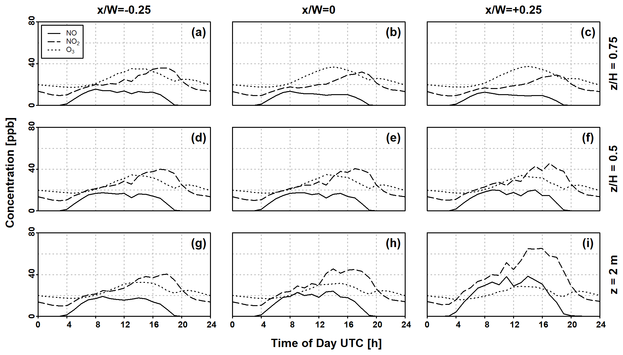
Figure 12Hourly averaged time series of NO, NO2, and O3 concentrations at (a–c) , (d–f) , and (g–i) z=2 m at different horizontal stations over a 24 h period. The solar zenith angle (χ) crosses the 90∘ threshold at 02:35 and 19:25 UTC.
Finally, Fig. 12 shows the diurnal cycles in the concentrations of NO, NO2, and O3 in the street canyon from the transient model run at nine different locations corresponding the intersections between the vertical (Fig. 8) and horizontal profiles (Figs. 9 to 11). Both the NO and O3 profiles exhibit a typical diurnal cycle, which show strong dependence on solar activity, since only the titration Reaction (R3) remains active before sunrise and after sunset (i.e., ), as previously pointed out. Thus, in conjunction with emission rates from traffic NOx during these times, a drastic reduction in NO can be seen. Further, the O3 concentration at all monitoring points follows the same tendency as the background O3 shown in Fig. 6c, except at the time immediately following the cessation of solar activity (at 19:25 UTC), where an acute reduction is observed due to NOx still presently available, mainly from emission sources, for the titration Reaction (R3).
While the trend of NO2 concentration in the afternoon and early evening (that is, between 15:00 and 21:00 UTC) is in line with the traffic emissions, the overall diurnal variation does not reflect the morning traffic peak but instead only gradually increases following sunrise at 02:35. As the morning period is accompanied by a comparatively low background O3 concentration, the photodissociation of NO2 becomes the dominant reaction in the mechanism, leading to consumption of the emitted NO2 from the traffic sources. As the O3 concentration increases in the afternoon, the rate of titration increases correspondingly. Therefore the afternoon NO2 peak coincides with a decrease in NO concentration.
A weakly compressible, reactive finite-volume LES solver, based on the OpenFOAM computational continuum mechanics framework (Weller et al., 1998), has been developed for modeling chemical transport of gas-phase pollutant species in an idealized street canyon under conditions where meteorology, background pollutant concentrations, and traffic emissions vary with time. A deep street canyon with a height-to-width aspect ratio of two (Zhong et al., 2015) has been used throughout this study. The solver has been evaluated using stationary LDA measurements from Li et al. (2008), showing excellent agreement in mean flow and turbulent velocity fluctuations. Whereas previous studies on street canyons have been conducted under stationary conditions, a subsequent transient model run with chemical transport, time-varying boundary conditions representing a typical working day for the city of Berlin in July 2014 covering a 24 h period have been prepared. Comparisons have also been made with stationary runs corresponding to certain points of time during the diurnal cycle. While vertical and horizontal profiles for velocity components indicate minor differences between the stationary runs and the transient runs at corresponding times, a large deviation in pollutant species concentration can be observed. This discrepancy is caused by time variations in ambient conditions, which also leads to differences in cumulative concentrations prior to solution sampling, both factors not considered in stationary runs. Diurnal variations in pollutant concentrations can also be inferred through the transient model run at specific locations in the canyon, showing typical profiles of NO, NO2, and O3 that correspond to traffic emissions, background concentrations, and solar zenith angle.
The results of this study demonstrate the ability of this solver in performing urban-scale chemistry transport modeling in both a stationary and non-stationary capacity in a grid-independent manner. As such, it can be readily adapted to model a larger domain with more realistic geometry, such as a city block. For models covering such domain regions, however, input data such as meteorology and emission profiles need to be prescribed at higher spatial and temporal resolutions, which can be accomplished by coupling the urban scale model with outputs from regional models, e.g., WRF-Chem. Particular emphasis can be placed on the role of absorptive, reflective, and refractive mechanisms of urban structures in the redistribution of solar radiant energy and their impact on the overall advective and convective thermal stratification in their immediate vicinity.
Further, the method of spatiotemporal distribution and NOx
emissions from annual aggregate and the subsequent partition into NO
and NO2 contributions, as outlined in Sect. 4.1,
can be extended to cover a road network, where emissions can be mapped as
discretized surface fluxes in a similar manner as the simpleEmission
boundary condition described in Sect. 2.3.
In addition to NOx, the emissions of PM, carbon
monoxide (CO), and volatile organic compounds (VOCs)
can be processed in a similar way.
While the photostationary NO-NO2-O3
mechanism (Leighton, 1961) serves as the integral component of the OpenFOAM
chemistry model for the current study, modeling transformation processes
of CO and VOCs will certainly require chemical kinetics that include
reactions of these species and their intermediate derivatives, such as
OH, R-H, and R-O2.
Mechanisms such as CBM-IV (Gery et al., 1989), involving 32 species and 81 reactions,
or, to a lesser degree, the SMOG mechanism (Damian et al., 2002), made up of 13 species
and 12 reactions, can be considered in subsequent investigations.
A1 Roman symbols
| ai | Polynomial coefficient for the ith power term |
| A | Arrhenius pre-exponential factor, in units of [m, kmol, s, K] |
| AS | Sutherland law reference viscosity factor [kg m−1 s−1 K] |
| Ck | Parametric constant for SGS viscosity [] |
| Cϵ | Parametric constant for SGS TKE dissipation rate [] |
| cp | Specific heat at constant pressure [J K−1 kg−1] |
| D | Binary diffusion coefficient [kg m−1 s−1] |
| e | Internal energy [J] |
| g | Gravitational acceleration [m s−2] |
| h | Enthalpy [J] |
| h | Planck constant (in Reaction R1) [J s] |
| i, j, k, q | Generic indices |
| J0 | Photolysis rate at χ=0 [s−1] |
| jR | Photolysis rate [s−1] |
| k | Turbulent kinetic energy [m2 s−2] |
| kR | Reaction rate constant [m3 kmol−1 s−1] |
| m, n | Photolysis rate parameters [] |
| p | Pressure [Pa] |
| R | Specific gas constant [J K−1 kg−1] |
| r | Net species production rate [m3 s−1] |
| Sij | Shear strain rate tensor [s−1] |
| T | Temperature [K] |
| TA | Arrhenius activation temperature [K] |
| TS | Sutherland law reference temperature [K] |
| U | Reference velocity [m⋅s-1] |
| u, v, w | Velocity components [m s−1] |
| u′, v′, w′ | Velocity fluctuation [m s−1] |
| x, y, z | Cartesian coordinate [m] |
| yq | Mass mixing ratio for species q [] |
A2 Greek symbols
| Δ | Subgrid filter length scale [m] |
| δx | Local grid size [m] |
| δij | Kronecker delta [] |
| ϵijk | Permutation tensor [] |
| λ | (Photon) wavelength [m] |
| μ | Dynamic viscosity [Pa s] |
| ν | (Photon) vibrational frequency [s−1] |
| ξ | Cartesian coordinate (alternative to x) [m] |
| ρ | Density [kg m−3] |
| SGS term for scalar φ | |
| τij | Shear stress tensor [Pa] |
| ϕ | Latitude [] |
| φ | Generic scalar variable |
| χ | Solar zenith angle [] |
| ω | Angular velocity [s−1] |
A3 Mathematical operators
| dx(⋅) | Direct derivative: |
| Partial derivative: | |
| Partial derivative (shorthand): | |
| Dt(⋅) | Substantial derivative: |
| F(x|Δ) | Spatial low-pass filter kernel with cut-off length Δ |
| [φ] | Volumetric concentration |
| Temporal (RANS) average | |
| 〈φ〉 | Spatial average |
| Density-weighted (Favre) average: |
A4 Acronyms and abbreviations
| BLUME | Berlin Air Quality Measurement Network (Berliner Luftgüte-Messnetz) |
| CBM | Carbon bond mechanism |
| DNS | Direct numerical simulation |
| GNFR | Gridding nomenclature for reporting |
| ILU | Incomplete lower–upper (matrix factorization) |
| LDA | Laser Doppler anemometry |
| LES | Large-eddy simulation |
| PM | Particulate matter |
| RANS | Reynolds-average Navier–Stokes (equations) |
| RCS | Reduced chemical scheme |
| SGS | Subgrid scale |
| TKE | Turbulent kinetic energy |
| VOC | Volatile organic compound |
| WRF | Weather Research and Forecasting (Model) |
The exact version of urbanChemFoam and all components
described in Sect. 2.3, as well as select test cases
featured in this article, are licensed under the terms of the
GNU General Public License version 3.0 or later and can be obtained
using the following digital object identifier: https://doi.org/10.5281/zenodo.4384731 (Chan and Butler, 2020).
The supplement related to this article is available online at: https://doi.org/10.5194/gmd-14-4555-2021-supplement.
The activities outlined in this article have been conceived and
designed by ECC and TMB. ECC was responsible for the development
of urbanChemFoam and all related components, execution of all model
runs, and preparation of the manuscript. TMB provided technical and scientific
input at all stages of the study.
The authors declare that they have no conflict of interest.
Publisher's note: Copernicus Publications remains neutral with regard to jurisdictional claims in published maps and institutional affiliations.
The BLUME urban background concentration station measurements and the aggregated annual traffic emissions data have been provided by the Senate Administration for Environment, Traffic, and Climate Protection (Senatsverwaltung für Umwelt, Verkehr und Klimaschutz) of the city of Berlin. The stationary LDA measurement data of Li et al. (2008) have been made available by Jian Zhong and Xiaoming Cai from the University of Birmingham. The authors would also like to express their gratitude to IASS colleagues Joana Leitão, Aurelia Lupaşcu, and Jörn Quedenau for their valuable input and support in the conception and preparation of this work.
This paper was edited by Christoph Knote and reviewed by two anonymous referees.
Baik, J. J. and Kim, J. J.: A Numerical Study of Flow and Pollutant Dispersion Characteristics in Urban Street Canyons, J. Appl. Meteorol., 38, 1576–1589, 1998. a, b, c
Baker, J., Walker, H. L., and Cai, X.: A study of the dispersion and transport of reactive pollutants in and above street canyons – a large eddy simulation, Atmos. Environ., 38, 6883–6892, 2004. a
Bright, V. B., Bloss, W. J., and Cai, X.: Modelling atmospheric composition in urban street canyons, Weather, 66, 106–110, 2011. a
Bright, V. B., Bloss, W. J., and Cai, X.: Urban street canyons: Coupling dynamics, chemistry and within-canyon chemical processing of emissions, Atmos. Environ., 68, 127–142, 2013. a
Britter, R. E. and Hanna, S. R.: Flow and Dispersion in Urban Areas, Annu. Rev. Fluid Mech., 35, 469–496, 2003. a
Burkholder, J. B., Sander, S. P., Abbatt, J., Barker, J. R., Huie, R. E., Kolb, C. E., Kurylo, M. J., Orkin, V. L., Wilmouth, D. M., and Wine, P. H.: Chemical Kinetics and Photochemical Data for Use in Atmopsheric Studies, Evaluation No. 18.. JPL Publication 15-10, Jet Propulsion Laboratory, Pasadena, CA, 2015. a
Cabral, B. and Leedom, L. C.: Imaging vector fields using line integral convolution, in: Proceedings the 20th annual conference on computer graphics and interactive techniques, Association for Computing Machinery, Anaheim, CA, 263–270, 1993. a
Carpenter, L. J., Clemitshaw, K. C., Burgess, R. A., Penkett, S. A., Cape, J. N., and McFadyen, G. G.: Investigation and Evaluation of the NOx/O3 Photochemical Steady State, Atmos. Environ., 32, 3353–3365, 1998. a
Chan, E. C. and Butler, T. M.: Code and data set for GMD-2020-432 (Version 1.0) [code and data set], Zenodo, https://doi.org/10.5281/zenodo.4384731, 2020. a
Chevalier, C. and Pellegrini, F.: PT-Scotch: A tool for efficient parallel graph ordering, Parallel Comput., 34, 318–331, 2008. a
Cranier, C., Darras, S., Denier van der Gon, H. A. C., Doubalova, J., Elguindi, N., Galle, B., Gauss, M., Guevara, M., Jalkanen, J.-P., Kuenen, J., Liousse, C., Quack, B., Simpson, D., and Sindelarova, K.: The Copernicus Atmosphere Monitoring Service global and regional emissions (April 2019 version), Copernicus Atmosphere Monitoring Service, Reading, 2019. a
Damian, V., Sandu, A., Damian, M., Potra, F., and Carmichael, G. R.: The Kinetic PreProcessor KPP – A Software Environment for Solving Chemical Kinetics, Comput. Chem. Eng., 26, 1567–1579, 2002. a
Davies-Jones, R.: Thermal convection in an infinite channel with no-slip sidewalls, J. Fluid Mech., 44, 695–704, 1970. a, b
Deardorff, J. W.: Stratocumulus-capped mixed layers derived from a three-dimensional model, Bound.-Lay. Meteorol., 18, 495–527, 1980. a
Driver, D. M. and Seegmiller, H. L.: Features of a Reattaching Turbulent Shear Layer in Divergent Channel Flow, AIAA Journal, 23, 163–171, 1985. a, b
EEA: European Union emission inventory report 1990–2017 under the UNECE Convention on Long–range Transboundary Air Pollution (LRTAP). EEA Report 8/2019, European Environmental Agency, Copenhagen, 2019a. a, b
EEA: Air Quality in Europe – 2019 report. EEA Report 10/2019, European Environmental Agency, Luxembourg, 2019b. a, b
Favre, A.: Équations des gaz turbulents compressible. II. Méthode des vitesses moyennes, méthode des vitesses macroscopiques pondérées par la masse volumique, J. Mécanique, 4, 391–421, 1965. a
Garmory, A., Kim, I. S., Britter, R. E., and Mastorakos, E.: Simulations of the dispersion of reactive pollutants in a street canyon, considering different chemical mechanisms and micromixing, Atmos. Environ., 43, 4670–4680, 2009. a
Garnier, E., Adams, N. A., and Sagaut, P.: Large eddy simulation for compressible flows, Springer, Dordrecht, 2009. a
Gery, M. W., Whitten, G. Z., Killus, J. P., and Dodge, M. C.: A photochemical kinetics mechanism for urban and regional scale computer modeling, J. Geophys. Res., 94, 12925–12956, 1989. a, b
Huie, R. E., Herron, J. T., and Davis, D. D.: Absolute rate Constants for the Reaction O + O2 + M → O3 + M over the Temperature Range 200–346 ∘K, J. Phys. Chem., 76, 2653–2658, 1972. a
Kim, J. J. and Baik, J. J.: Urban street-canyon flows with bottom heating, Atmos. Environ., 35, 3395–3404, 2001. a
Kristóf, G., Papp, B., Wang, H., and Hang, J.: Investigation of the flow and dispersion characteristics of repeated orogrpaphic structures by assuming transient wind forcing, J. Wind Eng. Ind. Dyn., 197, 104087, https://doi.org/10.1016/j.jweia.2019.104087, 2020. a
Kuik, F., Lauer, A., Churkina, G., Denier van der Gon, H. A. C., Fenner, D., Mar, K. A., and Butler, T. M.: Air quality modelling in the Berlin–Brandenburg region using WRF-Chem v3.7.1: sensitivity to resolution of model grid and input data, Geosci. Model Dev., 9, 4339–4363, https://doi.org/10.5194/gmd-9-4339-2016, 2016. a
Kuik, F., Kerschbaumer, A., Lauer, A., Lupascu, A., von Schneidemesser, E., and Butler, T. M.: Top–down quantification of NOx emissions from traffic in an urban area using a high-resolution regional atmospheric chemistry model, Atmos. Chem. Phys., 18, 8203–8225, https://doi.org/10.5194/acp-18-8203-2018, 2018. a, b
Kwak, K. H. and Baik, J. J.: Diurnal variation of NOx and ozone exchange between a street canyon and the overlying air, Atmos. Environ., 86, 120–128, 2014. a, b
Leighton, P. A.: Photochemistry of Air Pollution, Academic, Cambridge, MA, 1961. a, b, c
Leonard, A.: Energy Cascade in Large-Eddy Simulations of Turbulent Fluid Flows, Adv. Geophys., 18, 237–248, 1974. a
Li, X. X., Leung, D. Y. C., Liu, C. H., and Lam, K. M.: Physical Modeling of Flow Field inside Urban Street Canyons, J. Appl. Meteorol. Climatol., 47, 2058–2067, 2008. a, b, c, d, e, f, g, h
Liu, C. H., Leung, D. Y. C., and Barth, M. C.: On the prediction of air and pollutant exchange rates in street canyons of different aspect ratios using large-eddy simulations, Atmos. Environ., 39, 1567–1574, 2005. a
Madalozzo, D. M. S., Braun, A. L., Awruch, A. M., and Morsch, I. B.: Numerical simulation of pollutant dispersion in street canyons: Geometric and thermal effects, Appl. Math. Model., 24, 5883–5909, 2014. a
Martín, M. P., Piomelli, U., and Candler, G. V.: Subgrid-Scale Models for Compressible Large-Eddy Simulations, Theor. Comput. Fluid Dyn., 13, 361–376, 2000. a
McBride, B. J., Gordon, S., and Reno, M. A.: Coefficients for Calculating Thermodynamic and Transport Properties of Individual Species, NASA Technical Memorandum 4513, National Aeronautics and Space Administration, Cleveland, OH, 1993. a
Meeus, J.: Astromonical Algorithms, William-Bell, Richmond, VA, 1998. a
Minkos, A., Bauert, U., Feigenspan, S., and Kessinger, S.: Luftqualität 2019: Vorläufige Auswertung. ISSN 2363-829X, Umwelt Bundesamt, Dessau-Roßlau, 2020. a
OECD: The economic consequences of outdoor air pollution, OCED Publishing, Paris, 2016. a
Oke, T. R.: Street Design and Urban canopy Layer Climate, Energ. Buildings, 11, 103–113, 1988. a
Pope, S. B.: Turbulent Flows, Cambridge, 2000. a
Rhie, C. M. and Chow, W. L.: Numerical study of the turbulent flow past an airfoil with trailing edge separation, AIAA Journal, 21, 1525–1532, 1983. a
Saunders, S. M., Jenkin, M. E., Derwent, R. G., and Pilling, M. J.: Protocol for the development of the Master Chemical Mechanism, MCM v3 (Part A): tropospheric degradation of non-aromatic volatile organic compounds, Atmos. Chem. Phys., 3, 161–180, https://doi.org/10.5194/acp-3-161-2003, 2003. a
Skamarock, W. C., Klemp, J. B., Dudhia, J., Gill, D. O., Barker, D. M., Duda, M. G., Huang, X. Y., Wang, W., and Powers, J. G.: A Description of the Advanced Research WRF Version 3. NCAR Technical Note NCAR/TN-475+STR, National Center for Atmospheric Research, Boulder, CO, 2008. a
Smagorinsky, J.: General circulation experiments with the primitive equations: I: The Basic Experiment, Mon. Weather Rev., 91, 99–164, 1963. a
Tominaga, Y. and Stathopoulos, T.: Numerical simulation of dispersion around an isolated cubic building: Comparison of various types of k−ϵ models, Atmos. Environ., 43, 3200–3210, 2009. a
van der Vorst, H. A.: A Fast and Smoothly Converging Variant of Bi-CG for the Solution of Nonsymmetric Linear System, SIAM Journal on Scientific and Statistical Computing, 13, 631–644, 1992. a
von Schneidemesser, E., Kuik, F., Mar, K. A., and Butler, T. M.: Potential reductions in ambient NO2 concentrations from meeting Diesel vehicle emissions standards, Environ. Res. Lett., 12, 114025, https://doi.org/10.1088/1748-9326/aa8c84, 2017. a
Vreman, B., Geurts, B., and Huerten, H.: Subgrid-modeling in LES of compressible flow, Appl. Sci. Res., 54, 191–204, 1995. a
Weller, H. G., Tabor, G., Jasak, H., and Fureby, C.: A Tensorial approach to computational continuum mechanics using object-oriented techniques, Comput. Phys., 12, 620–631, 1998. a, b
Xie, X., Liu, C. H., and Leung, D. Y. C.: Impact of building facades and ground heating on wind flow and pollutant transport in street canyons, Atmos. Environ., 41, 9030–9049, 2007. a
Yoshizawa, A.: Statistical theory for compressible turbulent shear flows with the application to subgrid modelling, Phys. Fluids, 29, 2152–2164, 1986. a
Zhong, J., Cai, X., and Bloss, W. J.: Modelling the dispersion and transport of reactive pollutants in a deep urban street canyon: Using large-eddy simulation, Environ. Pollut., 200, 42–52, 2015. a, b, c, d