Development of a moving point source model for shipping emission dispersion modeling in EPISODE–CityChem v1.3

This paper demonstrates the development of a moving point source (MPS) model for simulating the atmospheric dispersion of pollutants emitted from ships under movement. The new model is integrated into the chemistry transport model EPISODE–CityChem v1.3. In the new model, ship parameters, especially speed and direction, are included to simulate the instantaneous ship positions and then the emission dispersion at different simulation time. The model was first applied to shipping emission dispersion modeling under simplified conditions, and the instantaneous and hourly averaged emission concentrations predicted by the MPS model and the commonly used line source (LS) and fixed point source (FPS) models were compared. The instantaneous calculations were quite different due to the different ways to treat the moving emission sources by different models. However, for the hourly averaged concentrations, the differences became smaller, especially for a large number of ships. The new model was applied to a real configuration from the seas around Singapore that included hundreds of ships, and their dispersion was simulated over a period of a few hours. The simulated results were compared to measured values at different locations, and it was found that reasonable emission concentrations were predicted by the moving point source model.

1 Introduction

Maritime transport plays an important role in the global transportation for passengers and goods. Compared to other transportation modes, such as road and air transport, maritime transport is considered as the most energy efficient and environment-friendly mode (International Maritime Organization (IMO), 2012). Maritime trade has grown rapidly in past years and is expected to keep an average annual growth rate of 3.5 % in the next 5 years (Asariotis et al., 2019), leading to an increase in maritime activities. As a result, pollutant emissions generated from ships keep increasing, and hence their impact on human health and environment in coastal cities and harbors has received attention from researchers (Langella et al., 2016; Tzannatos, 2010; Goldsworthy and Goldsworthy, 2015).

To evaluate the contributions of ship emissions on air quality in coastal areas, atmospheric dispersion modeling of the pollutants, such as NO_x, SO₂ and particulate matter (PM), in a regional or city scale by considering the local meteorological conditions, topographical information, turbulent diffusion and chemical transformations is a useful approach. Different dispersion software such as a Gaussian model and a Eulerian model have been developed and widely applied in numerical simulations (Milazzo et al., 2017; Gibson et al., 2013; De Nicola et al., 2013; Mallet et al., 2018; Kukkonen et al., 2016). The most common and simplest one is a Gaussian-based model that assumes the dispersion of air pollutant to follow a Gaussian distribution. Merico et al. (2019) applied a steady-state Gaussian-based model – ADMS-5 – to estimate the dispersion of emissions from ships which are mainly in the hoteling and maneuvering phase in the harbor area of an Italian port city of Bari. The same model was also used by Cesari et al. (2016) for a case study of ship emissions in Brindisi, Italy. Another popular steady-state Gaussian plume model, AERMOD, recommended by United States Environmental Protection Agency (EPA) was also widely used by different groups (Gibson et al., 2013; Cohan et al., 2011). Abrutytė et al. (2014) employed AERMOD to simulate the dispersion of NO_x from ships in Klaipėda port. AERMOD was also used by Fileni et al. (2019) and Cohan et al. (2011) to evaluate the contribution of ships on PM emissions in harbor cities. The Gaussian plume model is able to save a lot of computational cost; however, it suffers from several limitations, such as assuming a steady-state solution, a spatially uniform meteorology and straight line trajectories (Bluett et al., 2004), which make it not suitable under many conditions for air quality modeling. In addition to the simple Gaussian plume models, some advanced, unsteady Gaussian puff models (such as CALPUFF), which can simulate the effects of time- and space-varying meteorological conditions on pollutant transport, transformation and removal (Bluett et al., 2004), are developed as well. CALPUFF has been widely used for simulating the dispersion of ship emissions. Jahangiri et al. (2018) applied CALPUFF to predict the average values of the ship emissions on the port area of Brisbane, Australia, for the whole of 2013. Poplawski et al. (2011) and Murena et al. (2018) also employed CALPUFF to evaluate the effects of cruise ships on air quality in the harbors of Victoria, Canada, and Naples, Italy, respectively. Compared to the Gaussian plume models, the advanced unsteady Gaussian puff models overcome some limitations; for example, the causality effects can be simulated by CALPUFF.

Furthermore, a Lagrangian or Eulerian chemistry transport model (CTM) that solves the advection–diffusion equation and the atmospheric chemistry to predict the transport and chemical reactions of emission species received increasing attention (Pillai et al., 2012; Gariazzo et al., 2007; Gadhavi et al., 2015). For a Lagrangian CTM, a moving frame of reference is used to predict the trajectories of the pollution plume parcels. In comparison, an Eulerian CTM uses a fixed 3D Cartesian grid as the frame of reference to solve the continuity equations. Both CTMs have been applied to simulate the dispersion of ship emissions. Krysztofiak-Tong et al. (2017) evaluated the air pollution contributed from ships and oil platforms in West Africa by using the Lagrangian model FLEXPART. Shang et al. (2019) and Chen et al. (2018) applied the Eulerian-based WRF-Chem model to simulate the influence of ship emissions on harbor cities in China. Liu et al. (2017) studied the impact of ship emissions on the Shanghai urban area by using the WRF–CMAQ model. Huszar et al. (2010) evaluated the effects of ship emissions on NO_x and ozone (O₃) in the eastern Atlantic and Western Europe by using an Eulerian model CAMx. Karl et al. (2020) investigated the particle concentrations in the ship plumes by coupling an aerosol dynamic model MAFOR (Multicomponent Aerosol FORmation) with a 3D Eulerian chemistry transport model EPISODE–CityChem. In these studies, the chemistry transport models (mainly Eulerian models) have shown the ability of predicting the pollutant concentrations at the locations of interest and hence are a good approach for investigating the environmental impact of ship emissions in coastal cities.

In pollutant dispersion modeling, it is necessary to include an appropriate assumption or model for treating the emission sources. For a typical setup of shipping emission dispersion simulation, the definition for an emission source usually depends on the ship status, namely that the ship is at berth (hoteling) or on cruise (maneuvering and cruising). Usually, the ship at hoteling phase is treated as a fixed point emission source (Merico et al., 2019; Poplawski et al., 2011; Deniz and Kilic, 2010; Lucialli et al., 2011; Formentin, 2017), which is a reasonable assumption as the ship stops at the dock and generates emissions from its chimney as a single point. For the ships under movement, different models have been applied to treat the emission sources in different studies. Iodice et al. (2017) assumed the emissions from the moving ships were generated at multiple fixed points along the predefined navigation route. Saxe and Larsen (2004) used fixed points to represent the average positions of the ships in both maneuvering and hoteling modes. Murena et al. (2018) also treated the ships in maneuvering and navigation modes as fixed point emission sources. In another group of studies, a line emission source model was widely applied to simulate the moving ships in maneuvering or cruising mode (Poplawski et al., 2011; Kotrikla et al., 2013; Deniz and Kilic, 2010; Lucialli et al., 2011). In the line source (LS) model setup, the ship emission is assumed to be constantly emitted along the entire ship route, which is assumed to be a straight line. In some other cases, ships in hoteling or maneuvering modes were treated as area sources (Kotrikla et al., 2013; Formentin, 2017; Abrutytė et al., 2014); however, this assumption is not commonly used to treat ship emissions.

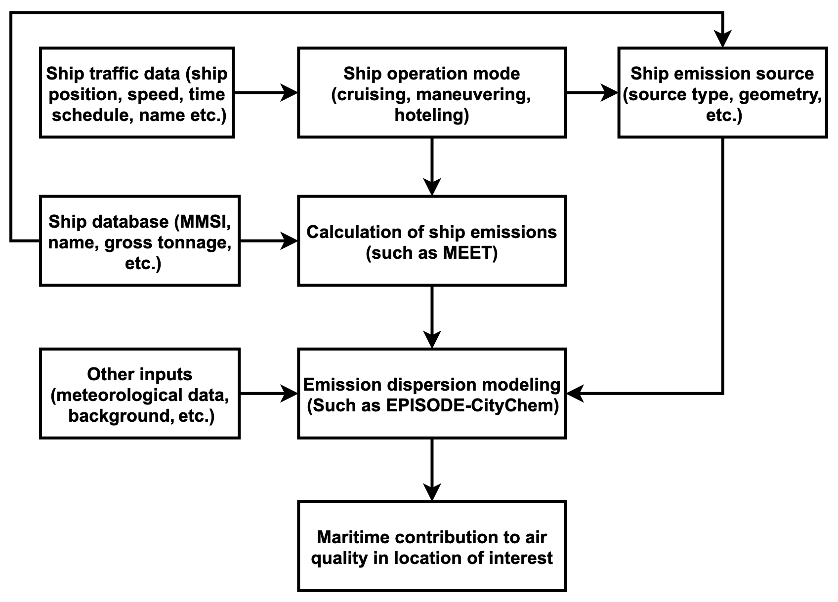
From the above literature review, it is evident that either a (or multiple) fixed point(s) source model or a line source model is commonly used for ships under movement in the air pollution dispersion modeling. However, neither of these assumptions is realistic as the ship position is changing when it is moving. The ship movement is not explicitly included in current air pollution dispersion modeling and leads to a research gap. In this paper, a moving point source (MPS) model that can update the ship positions at different times based on the ship speed and direction and then simulate the emission release from the moving ships in the dispersion modeling was hence developed. The new developed MPS model was integrated into the 3D Eulerian chemistry transport model EPISODE–CityChem (Hamer et al., 2020; Karl et al., 2019) and applied to predict the dispersion of NO₂ species generated by the ships in cruising mode in a simplified simulation, and the simulated results were compared to those obtained by using LS and fixed point source (FPS) models. In addition, the new MPS model was applied to a real case study to predict the concentrations of NO₂ and PM_2.5 species contributed by all ships around the city of Singapore, and the simulated results were compared to the measured values in different observation stations. The MPS model introduces a new approach for treating the ships and other objects under movement in the atmospheric dispersion modeling and will increase the knowledge of the atmospheric environment modelers. The model setups and important simulation results are presented in this paper.

2 Methods

The MPS model developed in this paper was integrated into the chemistry transport model, EPISODE–CityChem (Hamer et al., 2020; Karl et al., 2019), which is an open-source Fortran-based code. EPISODE–CityChem is a city-scale chemistry extension of the dispersion model EPISODE, which was originally developed by Slørdal et al. (2003) and Slørdal et al. (2008). In this section, the dispersion model, the MPS model, simulation setups and configurations of the case studies are introduced.

2.1 Dispersion model

EPISODE–CityChem simulates the transport, chemical reactions and deposition of pollutant species in both a 3D Eulerian grid and a ground-level sub-grid (Hamer et al., 2020; Karl et al., 2019). A typical Eulerian grid has a horizontal resolution of 1 km by 1 km, while the vertical grid size varies from several meters (near the ground) to several hundreds meters (higher layer), with a total height up to several kilometers. The sub-grid has a better resolution with a typical size of 100 m by 100 m horizontally. The governing advection–diffusion and mass conservation equations for the averaged concentrations in the main Eulerian grid model are indicated as

$$\begin{array}{}\text{(1)}& {\displaystyle }\begin{array}{rl}& {\displaystyle \frac{\partial C_i}{\partial t}}+{\displaystyle \frac{\partial \left(u{C}_i\right)}{\partial x}}+{\displaystyle \frac{\partial \left(v{C}_i\right)}{\partial y}}+{\displaystyle \frac{\partial \left(w{C}_i\right)}{\partial z}}=\\ & {\displaystyle \frac{\partial }{\partial x}}\left(K^{\left(H\right)}{\displaystyle \frac{\partial C_i}{\partial x}}\right)+{\displaystyle \frac{\partial }{\partial y}}\left(K^{\left(H\right)}{\displaystyle \frac{\partial C_i}{\partial y}}\right)\\ & +{\displaystyle \frac{\partial }{\partial z}}\left(K^{\left(z\right)}{\displaystyle \frac{\partial C_i}{\partial z}}\right)+R_i-S_i,\end{array}\text{(2)}& {\displaystyle \frac{\partial u}{\partial x}}+{\displaystyle \frac{\partial v}{\partial y}}+{\displaystyle \frac{\partial w}{\partial z}}=\mathrm{0},\end{array}$$

where C_i is the concentration of species i ($i=\mathrm{1}:N$, where N is the total number of species); u, v and w are the three wind velocity components; K^(H) and K^(z) are the horizontal and vertical eddy diffusivities; and R_i and S_i represent the source and sink terms. The estimation of eddy diffusivities is based on the mixing length theory (K-theory) (Slørdal et al., 2003). In the simulation, the emission source term, wind field and other meteorological conditions are assumed to be hourly constant. The emission species is simulated until it is fully diluted or outside of the simulation domain. The photochemistry simulated in the Eulerian grid has several options, such as EMEP45 (Walker et al., 2003), EmChem03mod and EmChem09mod (Simpson et al., 2012), that are modified or updated from the European Monitoring and Evaluation Programme (EMEP) (Simpson, 1995). In this study, the chemical scheme applied is EmChem09mod.

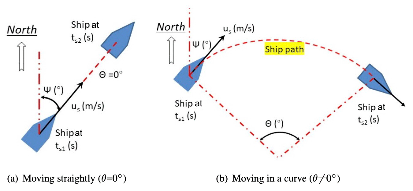
Figure 1 Illustration of the moving point source model. The ship variables in the figures are explained in Table 1.

Table 1 Setup of the moving point source model.

Note that in each simulation hour, all five variables are assumed constant and only need to be updated hourly.

In the sub-grid receptor model, the pollutants generated by emission sources (either a point or a line source) are calculated by using simple Gaussian models. The LS model used in the EPISODE–CityChem package is a steady-state integrated Gaussian plume model (HIWAY-2) with a simplified street canyon model (SSCM), which affects the concentrations on the receptor points close to the line source (usually within an influence distance of 500 m). The emitted mass from line sources is integrated into the 3D Eulerian model in each simulation time step. For the point source, a Gaussian segmented plume model, SEGPLU (Walker and Grønskei, 1992), with the use of a Weak-wind Open Road Model (WORM) (Walker, 2011) meteorological pre-processor (WMPP) is implemented to treat the pollutants released from an individual point source as discrete emissions of finite length plume segments that emitted in each time interval (Δt). In the calculations, the plume rise (due to buoyancy or momentum) is estimated based on Briggs’s algorithms (Briggs, 1969, 1971, 1975), which consider the different atmospheric stability conditions (such as neutral-unstable and stable conditions). The effects of stack downwash (Briggs, 1973) and plume penetration (Weil and Brower, 1984) on plume height are considered as well. The transport, growth, chemical reaction and deposition of the plumes are estimated based on the local meteorological conditions where the plumes stay, and the plume mass is integrated into the Eulerian grids when the segmented plume grows to a predefined size (usually when ${\mathit{\sigma }}_y/\text{d}y=\mathrm{4}$ or ${\mathit{\sigma }}_z/\text{d}z=\mathrm{4}$, where σ_y and σ_z are Gaussian dispersion length scales in the cross-wind direction and the vertical direction for a plume, and dy and dz are the horizontal and vertical sizes of an Eulerian grid cell). The existing plumes contribute to the concentrations in the sub-grid receptors. The emission concentration at the receptor points is finally estimated as the sum of the Eulerian grid concentration and contributions from line and point sources, described as Eq. (3).

$$\begin{array}{}\text{(3)}& {\displaystyle }{\displaystyle }{C}_{\text{rec}}^t=C_{\text{m}}^{t-\mathrm{1}}+\sum _{l=\mathrm{1}}^L{C}_{\text{l}}^t+\sum _{p=\mathrm{1}}^P{C}_{\text{p}}^t,\end{array}$$

where $C_{\text{rec}}^t$ is the receptor point concentration at time t, $C_{\text{m}}^{t-\mathrm{1}}$ is the Eulerian grid concentration at the previous time step (estimated by Eq. 1), $C_{\text{l}}^t$ and $C_{\text{p}}^t$ are the concentrations contributed from line and point emission sources, and L and P are the total numbers of line and point emission sources. In the sub-grid modeling, the stack downwash, dry and wet deposition, and plume rise and penetration are considered as well, and the photochemistry applied is the EP10-Plume scheme (Karl et al., 2019). More details about the EPISODE–CityChem software can be found in the papers written by Hamer et al. (2020) and Karl et al. (2019).

2.2 The moving point source model

As found from the literature review, LS and FPS models are the common approaches to simulate the emissions generated by the moving ships; however, they are not realistic as they cannot update the instantaneous ship positions. The MPS model is hence developed to fill the gap in the pollutant dispersion modeling.

In the MPS model, five new parameters are defined to determine the ship movement route, as presented in Fig. 1. The most important parameters are ship speed and direction, which can be easily captured from the maritime online databases, such as MarineTraffic. Three additional parameters, namely turning angle, start and stop time, are defined to provide the options to customize the ship movement when more accurate ship travel information is obtained. The new variables for each ship are only updated hourly and hence kept constant for each simulation hour. The detailed descriptions about the five model parameters are summarized in Table 1.

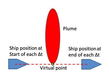
Based on these five variables, the ship position is estimated and updated in each simulation time step (Δt). As shown in Fig. 2, ship emission is assumed to be emitted in a virtual point of the short ship line that represents an average ship position for each individual time step. The emitted plume is then treated by using the SEGPLU model in EPISODE. As mentioned above, the parameters (such as plume size and location) of each individual plume were updated in each time step, and then their contributions to the 3D Eulerian cell and sub-grid receptors were calculated. In this model, the ship movement parameters, mainly ship speed, direction and turning angle, are constant for each simulation hour, and hence the virtual point is usually taken as the middle point of the short travel distance during each Δt. Apparently, the ship and plume positions are more realistic when the time step is smaller. For the time step in which the ship starts or stops moving, the estimation of the virtual point takes the time factor into account, as presented in Eqs. (4) and (5).

$$\begin{array}{}\text{(4)}& {\displaystyle }& {\displaystyle }{\mathit{x}}_i={\mathit{x}}_{i-\mathrm{1}}+\mathrm{0.5}\text{d}{\mathit{x}}_i{\displaystyle \frac{t_i-t_{s\mathrm{1}}}{\mathrm{\Delta }t}};(\text{if}{t}_{i-\mathrm{1}}\le t_{s\mathrm{1}}\le t_i),\text{(5)}& {\displaystyle }& {\displaystyle }{\mathit{x}}_i={\mathit{x}}_{i-\mathrm{1}}+\text{d}{\mathit{x}}_i-\mathrm{0.5}\text{d}{\mathit{x}}_i{\displaystyle \frac{t_{s\mathrm{2}}-t_{i-\mathrm{1}}}{\mathrm{\Delta }t}};(\text{if}{t}_{i-\mathrm{1}}\le t_{s\mathrm{2}}\le t_i),\end{array}$$

where x_i is the virtual position (x,y) of a ship during the ith time step in each simulation hour, $\text{d}{\mathit{x}}_i={\mathit{u}}_{\text{s}}(t_i-t_{s\mathrm{1}})$ (or ${\mathit{u}}_{\text{s}}(t_{s\mathrm{2}}-t_{i-\mathrm{1}})$) is the actual ship travel distance in the ith time step, t_i=iΔt is the actual time difference from the start of each simulation hour for the ith time interval and u_s is the ship velocity. As mentioned above, the five parameters in the simulation are only updated each hour, assuming that the ship is moving in a straight line or a curve with a constant speed during each hour. This is actually a limitation for the current version of the MPS model compared to a real ship if its movement parameters change frequently; however, the model used in this study is to address the idea of a MPS model that has the potential of tracking the ship movement and then better simulates the dispersion details of ship emissions. The current version of MPS model provides an alternative option for simulating the dispersion of ship emissions in a harbor city. In addition, it should be highlighted that it is possible to define an arbitrary ship movement by using the MPS model, once the real ship movement data collected at different time are added to the MPS input files in the simulation. In this study, the turning angle (θ) is set as 0^∘ for all moving ships, and the start time (t_s1) and stop time (t_s2) for all moving ships are assumed to be 0 and 3600 s respectively, due to the lack of such information for each ship.

Figure 2 Virtual point for plume release in each time step (Δt).

2.3 Simulation setup

The purpose of this study is to evaluate the new developed MPS model, and two simulations are conducted in the Singapore area in this paper. One is a simplified dispersion simulation that only includes moving ships with simplified input conditions, and the results by using the MPS model are compared with the LS and FPS models. Another is a real case study that simulates all the ships around the city of Singapore using the new model and compares them with the concentrations of emission species measured in different stations.

2.3.1 Simplified study

As shown in Fig. 3, the simulation is first conducted to include only a group of moving ships. The simulation domain is set for a 70 km by 70 km area, with a horizontal resolution of 1 km by 1 km in the reference case as suggested by Hamer et al. (2020) and Karl et al. (2019), and the domain has 13 vertical layers, with a height of 10 m in the ground layer and 500 m in the top layer (total height is 3500 m). The sub-grid receptor points (100 m by 100 m horizontal resolution) are created with a receptor height of 1.5 m above ground. In addition, a data point is selected around the coastline, as shown in Fig. 3, to record the concentrations of emission species at every simulation time step.

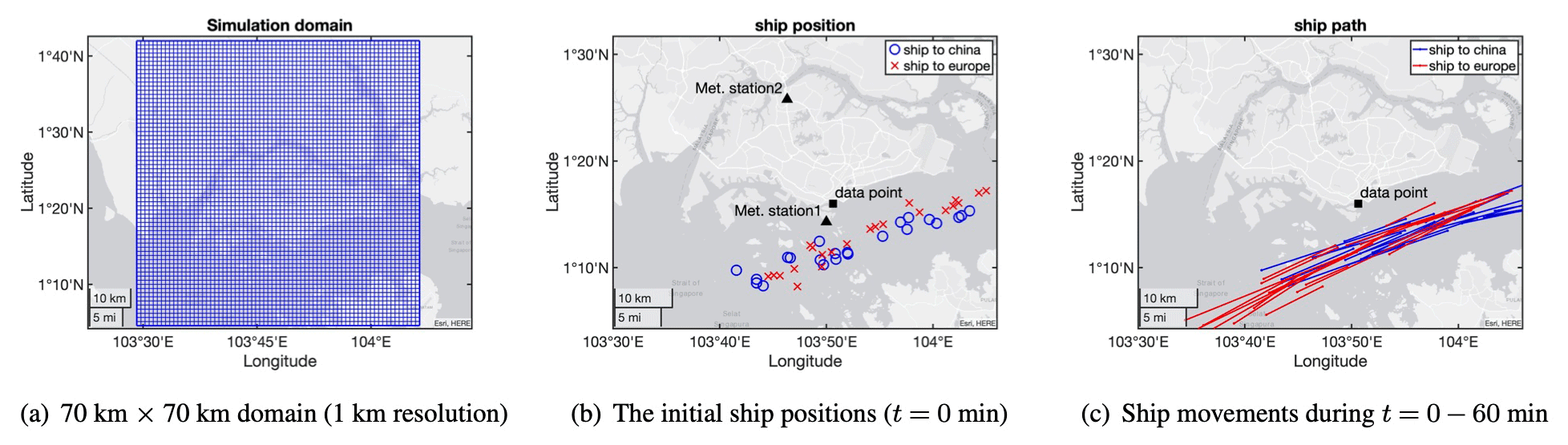
Figure 3 Configuration of the simulation domain in Singapore used in the simplified simulation. Ships to China are indicated by blue circles, and ships to Europe are indicated by red crosses; lines denote ship routes.

To simplify the simulation, a constant meteorological condition taken from two weather stations (as shown in Fig. 3b), one in the south of Singapore and another in the north of Singapore, was applied to the entire simulation period. The details of the weather conditions are shown in Table 2, where the wind inputs in two weather stations were assumed to be 2 m s⁻¹ and 180^∘ (blown from south to north). A built-in meteorological pre-processor, MCWIND, was used to first guess and estimate the local wind speed and direction in the simulation domain, based on the input values from the weather stations, and then they were adjusted to the given topography to obtain the 3D divergence-free and mass-consistent diagnostic wind field (Hamer et al., 2020). Other meteorological parameters (such as vertical temperature gradient) in the simulation area were also estimated by MCWIND. In this paper, the calculated wind field in the ground-level layer for the dispersion modeling is shown in Fig. 4.

Table 2 Meteorological inputs applied in MCWIND pre-processing utility for the simplified simulation.

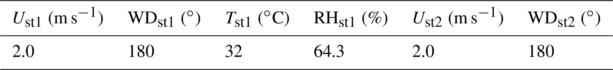
U: wind speed; WD: wind direction; T: temperature; RH: relative humidity; st1 and st2: weather station 1 and 2.

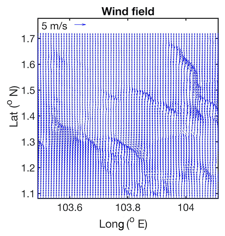
Figure 4 The 2D plot of ground-level diagnostic wind field calculated by MCWIND for the simplified dispersion modeling.

In the simplified simulation, a total number of 44 ships with different types and sizes are included. The ships are separated into two groups, where one group (22 ships) is assumed to move towards China and another is heading to Europe. The ship data, such as ship position, speed, direction and gross tonnage, are collected from online ship resources (such as VesselFinder). In order to better illustrate the feature of the new MPS model and also compare its results with those simulated by the LS and FPS models, only ships on the China–Europe route (west–east direction) are kept as the initial conditions by removing all other ships (such as those are at berthed or moving in a north–south direction), as shown in Fig. 3, and no new ships are included in the simulation. The dispersion modeling was conducted until all ships moved out of the simulation domain. During the entire simulation, all ships were assumed to move straightly (θ=0^∘), and the ship parameters (such as speed and direction) were assumed to be unchanged.

Table 3 Setups of shipping emission dispersion modeling.

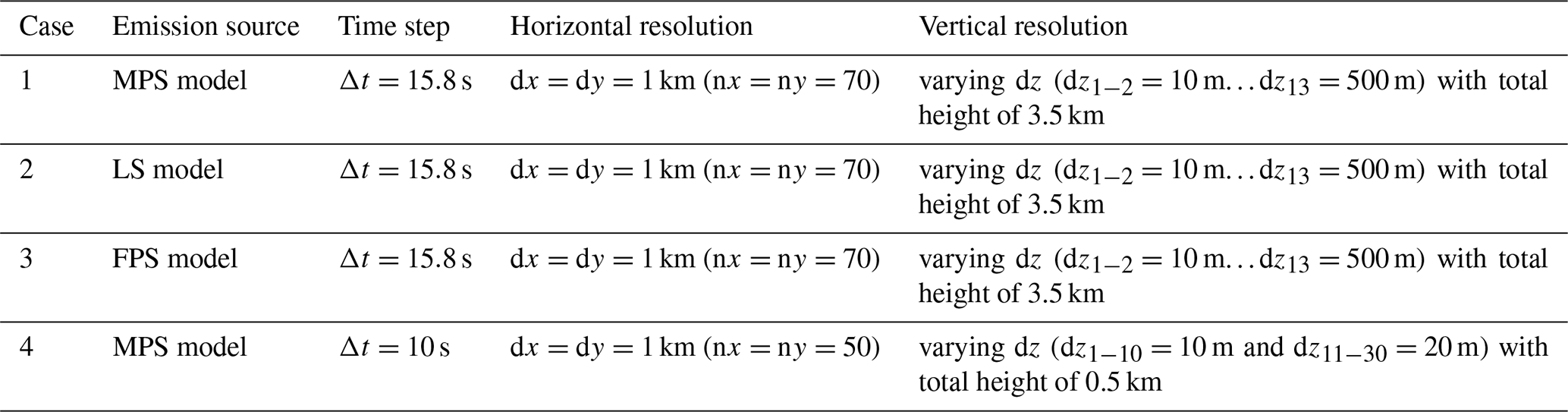
The ships are then divided into different categories (such as liquid bulk ships, dry bulk carriers, containers and cargo) based on those defined in the MEET (Methodologies for estimating air pollutant emissions from transport) methodology by Trozzi and Vaccaro (1999) and Trozzi (2010). The emission rates of main species (such as NO_x and PM) for each ship were then estimated by using the power-based emission factor equation (Eq. 6) proposed in the MEET method, based on a ship’s specifications such as ship type, speed and gross tonnage, as shown in Fig. 5. During the simplified simulation, the emission rates for each ship were constant as the ship operating conditions were unchanged, and no background concentrations were used. In addition, the chimney height is assumed to be 30 m for the large size ships (such as the liquid bulk ships) and 10 m for the small ones (such as the leisure ships), while exit gas is assumed to be at 20 m s⁻¹ with 300 ^∘C for all ships. The ship building height for each ship is set as 5 m below than the chimney height, and the width is assumed to be 20 m for the large-size ships and 5 m for the small ones. These choices have a very minor effect on the results (Appendix C). In this study, the ship emission sources were treated by using three different models, namely moving point, fixed point and line sources, and the simulated emission profiles were compared. The simulation setups are summarized in Table 3. In addition, sensitivity studies were conducted by changing the mesh density, simulation time step and emission source setups (such as exit velocity, chimney height and ship building dimensions), and the simulated concentration profiles for different species (such as NO₂, SO₂ and PM_2.5) were compared as well. The simulation results for the sensitivity studies are presented in Appendices A–D.

$$\begin{array}{}\text{(6)}& {\displaystyle }{\displaystyle }{E}_{\text{trip},i,j,k}=\sum _{\text{m}}\left[t_{\text{m}}\sum _e\left(P_e\times {\text{LF}}_e\times {\text{EF}}_{e,i,j,k,m}\right)\right],\end{array}$$

where E_trip is the emission over a trip (kg), EF is the emission factor (kg kWh⁻¹), LF is the engine load factor (%), P is the engine power (kW), t is time (hours), e is the engine category (main or auxiliary engine), i is the pollutant species (such as NO_x, PM), j is the engine type (slow-, medium- and high-speed diesel engine, gas turbine, and steam turbine), k is the fuel type (bunker fuel oil, marine diesel/gas oil, gasoline), m is the ship operation mode (cruising, hoteling, maneuvering).

Figure 5 Shipping emission dispersion modeling with MEET method (Trozzi, 2010).

2.3.2 Real case study

The MPS model was applied to a real case study in this paper as well. The hourly averaged emission values for several hours (11:00 to 16:00 on 23 April 2020) in Singapore were simulated by using the MPS model, and the results at different observation stations were compared to the measured data. The model setups (such as the grid size) and numerical methods (such as MEET method for emission rate calculation) are the same as those used in the simplified simulation, except for those (such as the meteorology and background concentrations) introduced in this section. The configurations and setups of the simulation are shown in Fig. 6.

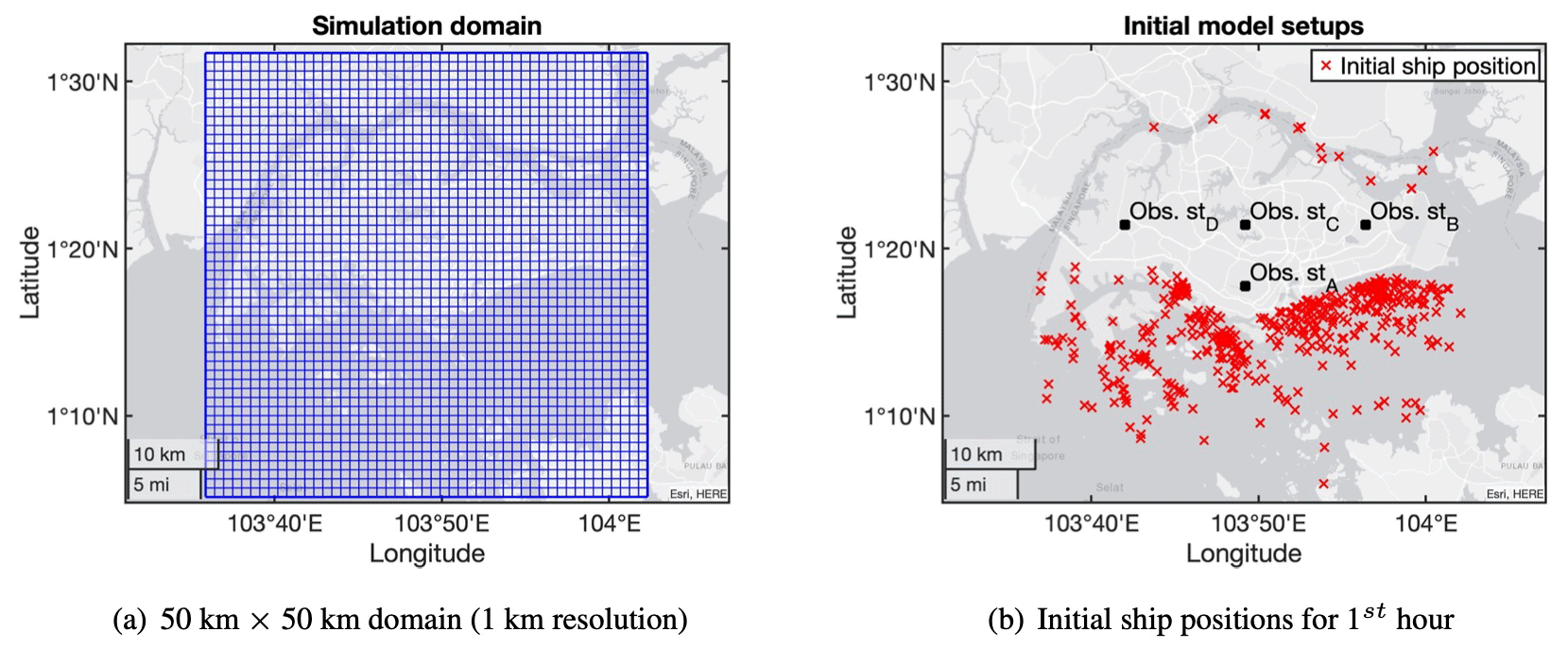
Figure 6 Configuration of the simulation domain used in the real case simulation.

The first difference in this real case study compared to the simplified simulation is that all the ships around the city of Singapore are included in the simulation, the ships are only updated each hour and their rates are estimated by using MEET method (Eq. 6) based on the ship information obtained from the online resource VesselFinder. Then the meteorological conditions obtained from Meteorological Service Singapore in each hour are applied to the simulation, while the concentrations of emission species obtained from the National Environment Agency in Singapore were selected as the background concentrations. In this study, all other model setups and configurations are listed as case 4 in Table 3.

3 Results and discussion

In this section, the results for two studies are presented. The first one (Sect. 3.1 and 3.2) results from comparing the MPS model with LS and FPS models for a simplified simulation. The air pollution dispersion modeling was first conducted with only one ship in the simulation domain, and the plume structures simulated by different emission models are compared. The emission source models were then applied to the additional simulation cases (cases 1–3) that include more ships in the China–Europe direction near Singapore. The instantaneous results and the hourly averaged NO₂ values simulated by different emission models are presented, as both of them are important for evaluating the impact of the pollutant emissions on the locations of interest. The second part (Sect. 3.3) is a real case study (case 4) that compares the predicted hourly averaged NO₂ and PM_2.5 concentrations by the MPS model at the observation stations with the measured data.

3.1 Simplified simulation – preliminary comparisons of different emission source models

The new MPS model was first tested by simulating only one ship, which moves from the east side to the west side. In this preliminary simulation, the ship movement parameters are constant, and all other conditions such as wind speed and direction are the same as mentioned in Table 2. Figure 7a presents the instantaneous NO₂ concentration near the ground simulated by the MPS model. Based on the 2D plots, it clearly shows that the species concentration inside the plume is gradually reduced in the opposed direction to the ship movement, which is reasonable. As the ship moves in the west–south direction and keeps emitting emissions at different positions along its route, the early generated emission are transported by wind further north and then diluted, and hence the emission plume is formed with minimum concentration on the east side and peak value on the west side. The simulated results indicate that the MPS model gives a quite reasonable prediction for the distribution of emissions released by a moving ship.

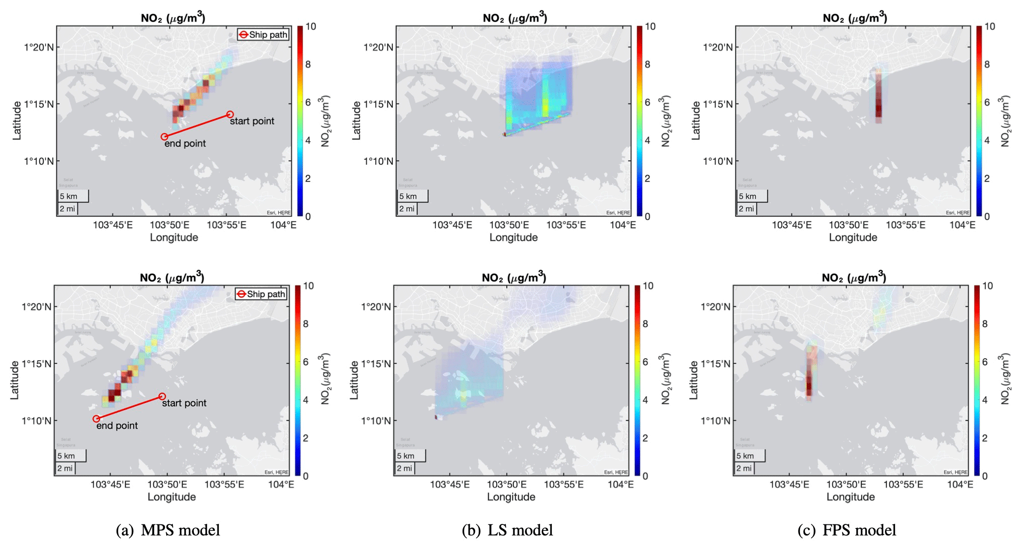
Figure 7 Instantaneous NO₂ concentrations near the ground generated by one moving ship. Top row: at t=60 min; bottom row: at t=120 min.

In comparison, the LS model gives quite different results, as shown in Fig. 7b, with the simulated NO₂ species distributed in a much wider area with a relatively smaller peak concentration. In the dispersion modeling, a line source is a very common model for treating a moving ship, assuming that the ship continuously generates emissions along the entire line in the simulation. As a result, more emissions appear near the entire ship route and are then gradually diluted in the downwind side. Compared to the real condition, it is unrealistic as the ship keeps moving and is not able to emit emissions from the entire ship route simultaneously. Furthermore, since the total emission rates (g s⁻¹) generated by the ship are the same for the MPS and LS models, the NO₂ emission rate at each point along the ship route (or emission rate intensity, g s⁻¹ m⁻¹) in the LS model is much smaller than the MPS model. Hence, the maximum NO₂ concentration generated by the LS model has a relatively smaller value than the MPS model.

In addition, the simulated emission profiles by using a FPS model are illustrated in Fig. 7c. The FPS model is another commonly used assumption for treating the moving ship in the literature. In this study, the moving ship is assumed to stay in the middle point of the ship routine in each hour. As shown in Fig. 7c, the NO₂ emission is blown north by wind from the ship point and then diluted. Since the ship position is assumed to be unchanged during each hour in the simulation, the emission is distributed in a much smaller area with a much larger concentration compared to the other two models. Clearly, the FPS model cannot reveal the effects of ship movement on emission dispersion.

3.2 Simplified simulation – results for case studies with more ships

After comparing the three emission source models for only one ship simulation, the three models were applied to a simplified study (cases 1–3) with 44 ships involved, in order to further evaluate the performance of different models for predicting the effects of moving ships on air quality in coastal cities. Both of the instantaneous and average results are presented in this section to fully compare the different emission models. The meteorological conditions and simulation setups are the same as presented in Tables 2 and 3.

3.2.1 Simulated results by using the moving point source model

In the case study for more moving ships, the simulation was first conducted by using the MPS model (case 1), and the instantaneous ground-level NO₂ concentrations at different time around the Singapore area are plotted in Fig. 8. Based on the 2D plots, it can be seen that the NO₂ emission moves north from the ship positions and forms the higher concentration at t=60 min compared to other simulation time, as most of ships are passing the same area during the first 60 min (Fig. 3c). The gas species then moves to the west and east directions as the two groups of ships move towards their destinations, and the gas concentration is continuously diluted in the following simulations as the ships keep moving out of the Singapore area.

Figure 8 Instantaneous NO₂ concentrations near the ground by using the MPS model (case 1).

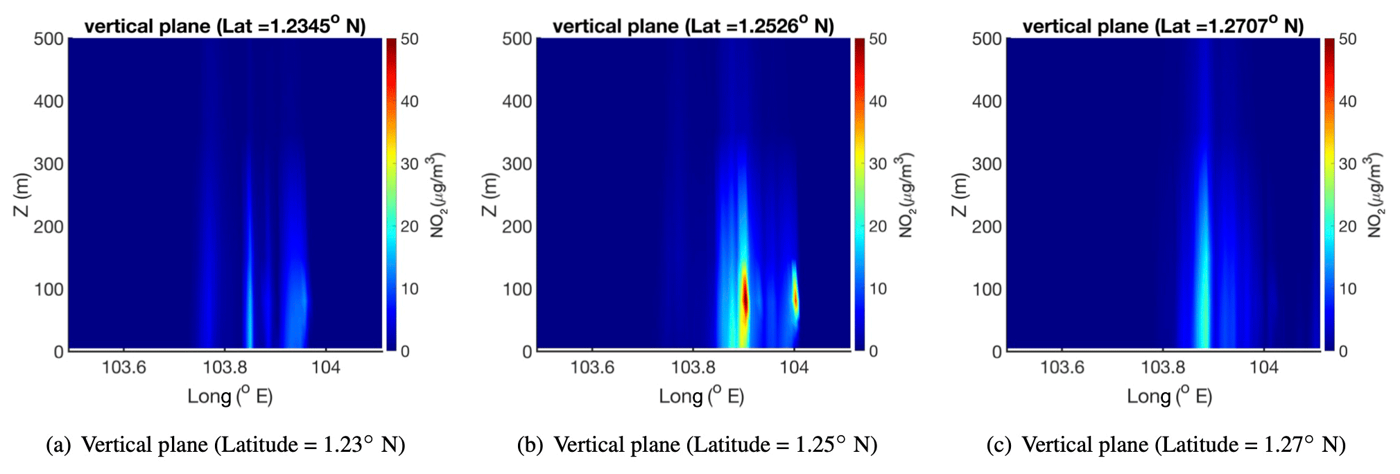
Figure 9 illustrates three vertical NO₂ concentration profiles (west–east vertical plane) at t=60 min. From these figures, it can be seen that less NO₂ species arrives on the ground when the plumes are closer to ships (Fig. 9a), and then the gas species are transported vertically to the ground as the plumes move in the downwind direction (Fig. 9b). This is mainly attributed to the plume rise effects when the gas species exits the ship chimney with a certain velocity (in the simplified simulation, the exit velocity is assumed to be 20 m s⁻¹ for all 44 ships), and then the gas species are blown by the wind (south to north) and only reach the ground at a certain distance in the downwind direction. As a result, the peak NO₂ concentrations at ground level appear on the locations that are far away from the ship routes but not near the ships, as shown in Fig. 8. As the emissions move further in the downwind direction, the plumes are diluted vertically until they fully disappear, as shown in Fig. 9c.

Figure 9 Vertical NO₂ profiles (west–east direction) at t=60 min.

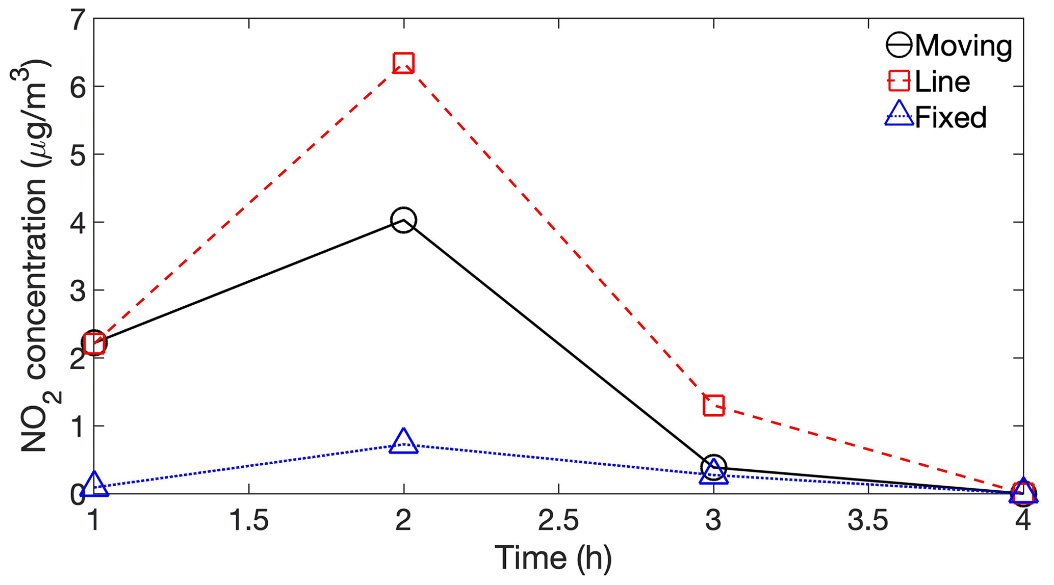
In addition, the time history of NO₂ concentration recorded at the data point (shown in Fig. 3b) is also plotted as shown in Fig. 10, where it indicates that there are two peaks for NO₂ concentration when using the MPS model. The time history is reasonable. Based on the NO₂ curves, it indicates that the emission species generated by the ships take around 30 min to reach the data point, and hence the two peaks should be induced by the transport and accumulation of emissions generated during the first 60 min. As shown in Fig. 11, a large group of ships pass by or are close to the data point during the first 30 min and lead to a continuous emission accumulation to form the first peak concentration, and another group of ships pass by the data point later (from 40 to 60 min) to generate the second peak value. After 60 min, most of the ships have passed the data point (Fig. 12), and hence the NO₂ concentration is continuously decreased. The time series of 2D plots in Fig. 8 and the NO₂ concentration curve in Fig. 10 reveal that the effects of ship movements on emission distributions can be well captured by using the MPS model.

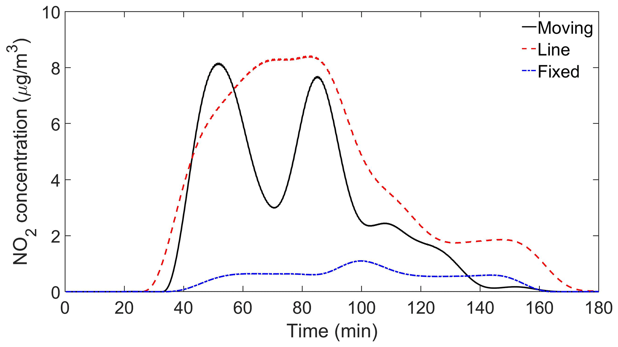
Figure 10 Time history of NO₂ concentration at the data point simulated by using different emission source setups.

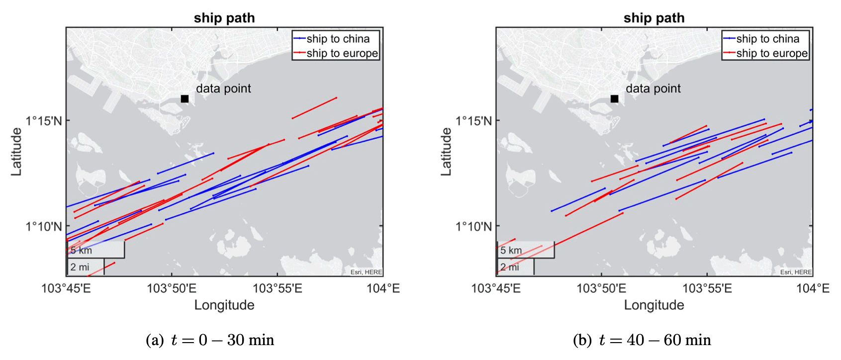
Figure 11 Ship movements during $t=\mathrm{0}-\mathrm{60}$ min.

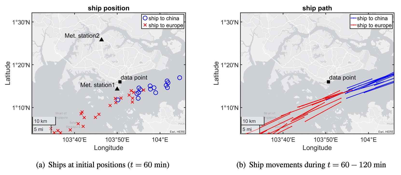
Figure 12 The ship initial positions and movements during t=60–120 min.

3.2.2 Comparison of three emission source models – instantaneous value

In the simplified case study, the simulation was then conducted by treating each moving ship as a line source (case 2). The instantaneous NO₂ concentrations contributed from the two groups of ships are plotted in Fig. 13 for different simulation times. Compared to the MPS results (Fig. 8), it clearly shows a much wider NO₂ distribution in the Singapore area when using the LS model to simulate the moving ships, due to the continuous emission generation along the entire ship routes. For the LS model, the generated emissions have the continuous impact on a specific area, while the emissions emitted by the MPS model only have transient impact on the same area. As a result, when ships are concentrated in a small region (as shown in Fig. 3), the integration of simulated NO₂ emission generated by line sources induces a higher peak concentration than the MPS model (Fig. 13a), although the emission rate intensity for each line source is smaller as mentioned in Sect. 3.1. As expected, when the ships are separated, the maximum NO₂ concentration for the line source becomes smaller than the MPS model, as shown in Fig. 13b and c.

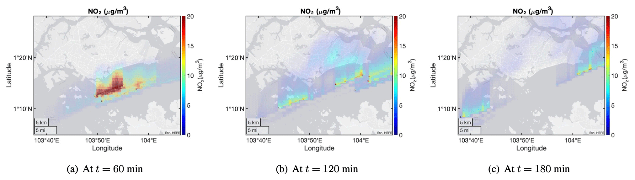
Figure 13 Instantaneous NO₂ concentrations near the ground by using the LS model (case 2).

The NO₂ time history curve for the LS simulation is also obtained as shown in Fig. 10. Compared to the MPS model, this simulated NO₂ concentration reaches its peak at around t=65 min and then is kept for around 15 min before it drops. In EPISODE–CityChem, hourly based simulations are conducted, and all the conditions such as meteorological parameters and emission setups are constant for every 60 min simulation. As shown in Figs. 3 and 12, more ships pass the data point during the first 60 min and less ships pass by during the second simulation period (t=60–120 min). When the LS model is used, a constant total NO₂ emission rate is generated during the first simulation period (t=0–60 min) and continuously affects the data point, leading to a concentration rise in the NO₂ curve to the peak value at around t=65 min (Fig. 10). Then the emission generation and dilution reach an equilibrium condition to maintain a constant peak concentration for a while, until the emissions generated by the ships in the second simulation period arrive at the data point. A smaller total emission rate is generated by the smaller amount of ships (during t=60–120 min) near the data point area, and hence the local concentration at the data point is reduced, shown as the NO₂ curve in Fig. 10. Clearly, the NO₂ concentration history obtained by the LS model cannot reveal the effects of real ship movements on emission dispersion, and hence it is not an appropriate assumption for simulating the instantaneous emission dispersion for ships in cruising mode compared to the MPS model.

In addition, the simulation was conducted by using the FPS model as well, assuming that the ships are staying at the middle points of the ship routes in each hour. The ground-level NO₂ distribution profiles are presented as Fig. 14. As expected, the emissions are distributed as separated plume segments, which are clearly not accurate. In Fig. 10, the NO₂ history curve for the fixed point assumption has the smallest peak value, as less NO₂ emission can be blown to the location of the data point. The individual plume segments and the smallest single-peak NO₂ time history indicate that the FPS model is an inaccurate approach for simulating the emission release and dispersion from the moving ships. Based on the comparisons of the simulation results by using three different emission models, this suggests that the new developed MPS model can simulate more realistic ship movement and then instantaneous emission concentrations generated by the moving ships.

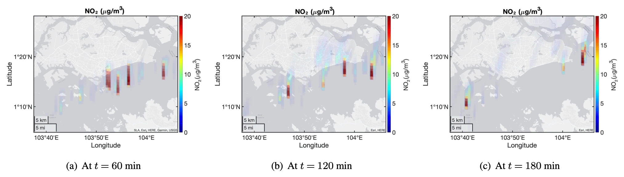
Figure 14 Instantaneous NO₂ concentrations near the ground by using the FPS model (case 3).

3.2.3 Comparison of three emission source models – average value

The simulation results in previous sections are the instantaneous NO₂ concentrations. In emission dispersion modeling, the average results (usually hourly based) are also important as they can be used for policy decision and for evaluating the long-term environmental impact. In this section, the hourly averaged results by using three different emission source models are compared as well, and the average NO₂ concentrations near the ground at different simulation time are presented in Fig. 15. Based on the 2D plots in Fig. 15, it can be seen that the average NO₂ profiles using the FPS model are much different from the other two setups. As discussed above, the FPS setup is clearly inappropriate for modeling the moving ships.

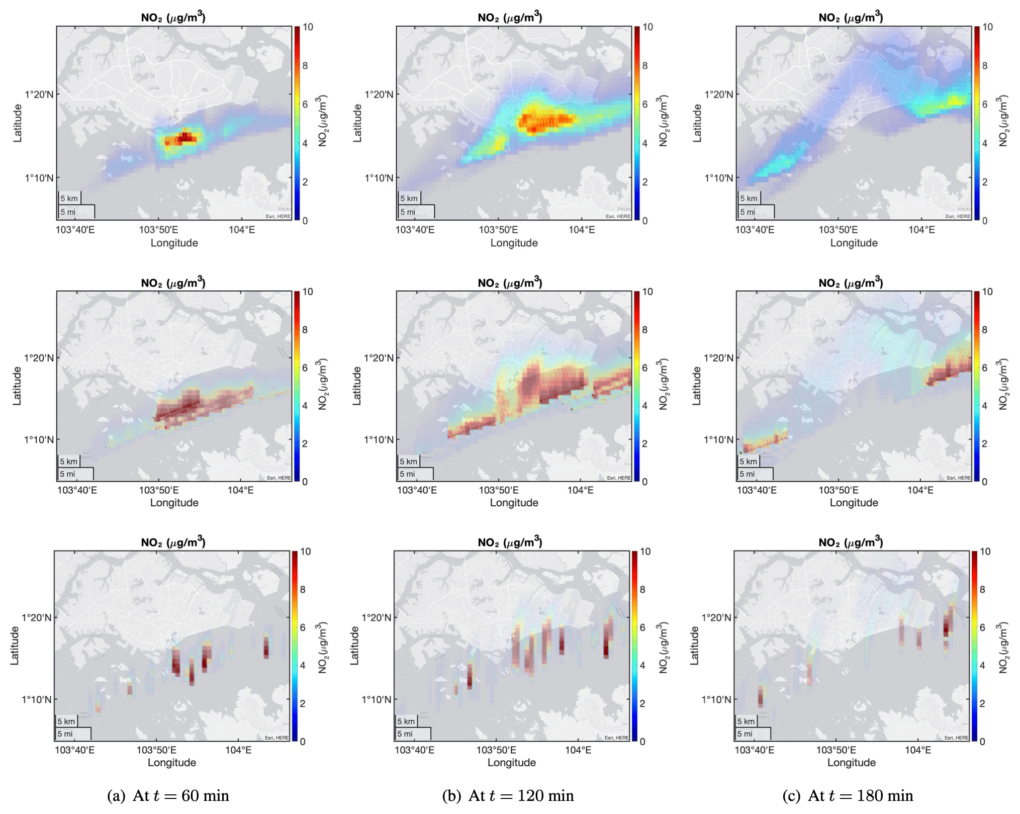
Figure 15 Hourly averaged NO₂ concentrations near the ground by using different emission models. Top row: MPS model (case 1); middle row: LS model (case 2); bottom row: FPS model (case 3).

The hourly averaged 2D plots in Fig. 15 also indicate that the simulated NO₂ emissions by using the MPS and LS models are distributed in a similar area. This is because the emissions for each ship are emitted along the same ship route for two models, although the location of NO₂ species generated by a MPS model changes along the ship route, while the LS model emits emissions along the entire route continuously. As a result, the accumulated NO₂ emissions cover a similar area for the two model setups and then generate similar results in the hourly averaged evaluations. However, the details of the NO₂ distributions (such as the peak concentration locations and values) are different for the two emission models, due to their natures of treating the emission generation differently in the dispersion modeling. As shown in Fig. 15, the LS model may overestimate the average NO₂ concentrations in some locations, compared to the MPS model.

The hourly averaged NO₂ concentrations at the data point for three emission source models are presented in Fig. 16. The concentration curves again indicate that the MPS and LS models predict comparable average NO₂ concentrations, while the FPS model gives a much different result. The simulation results suggest that the MPS model should be able to provide an alternative option to predict the hourly averaged emission concentrations and distributions in the air pollution dispersion modeling.

Figure 16 Hourly averaged NO₂ concentrations at a fixed point (“data point” in Fig. 3b) simulated by using different emission source setups.

3.3 Real case study – comparison with measurement

After comparing with the LS and FPS models in a simplified study, the new developed MPS model was applied to the real case by predicting the emission results generated by all ships (including those under cruise and at berth) around the Singapore area during a couple of hours. The predicted hourly averaged NO₂ and PM_2.5 concentrations are compared to the observed results obtained from the Singapore National Environment Agency online data resource.

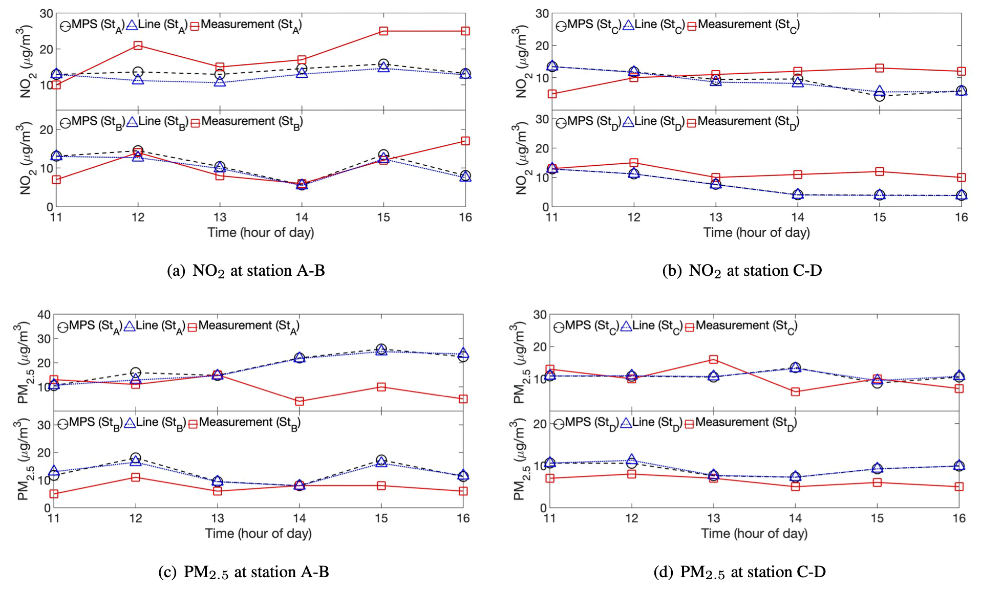
Figure 17 Comparison of hourly averaged emission concentrations between simulation and measurement at different locations.

Figure 17 compares the concentrations of NO₂ and PM_2.5 predicted by using the MPS model with the values obtained from different observation stations, whose locations are shown in Fig. 6b. Based on the figures, it can be seen that the new developed MPS model can reasonably predict the emission values at the four stations compared to the measured results, although there are still gaps between simulation and measurement. The differences may be attributed to the following aspects. First of all, only the emissions generated from ships around Singapore were included in the simulation; however, in the real world, the emissions measured in the observation stations should be the results contributed from ships and other sources, such as cars and powerplants. In addition, some assumptions were made in the simulation to simplify the model inputs that could induce different results from the real conditions. In the simulation, the meteorological conditions (such as wind speed and direction) are assumed to be hourly constant, although a space-varying wind field is estimated based on the input values at multiple weather stations, while the real wind and temperature are time- and space-varying, which could highly affect the dispersion of the emissions generated from ships. A constant background concentration was applied for the simulation while the actual value changes in different locations at different time. For the MPS model, each ship is assumed to move at constant speed and direction in each simulation hour, and no new ships are included until the next hour; however, in the real world, ships' speed and direction vary frequently, and ships can travel to the selected region at any time. The emission inventory or emission rate calculated by using the MEET method is based on the empirical equations fitted by the emission data obtained from a ship database, which includes ships with different types and sizes operating under different conditions (such as cruising and hoteling), and the estimated emission rates may be quite different from the actual values. Finally, the computational methods and model setups used in the simulation may not reveal the real process. The simulation is applied to a city-scale region with relatively coarse mesh setup, and the emission details at specific locations may not be well captured. The local emission distribution may vary highly due to the effects of different factors, such as building effect and different surface roughness. The chemical reactions of emission species are very complicated and may not be well predicted by the chemical mechanism applied in the simulation, while the physical changes in the aerosol particles are not simulated by the model.

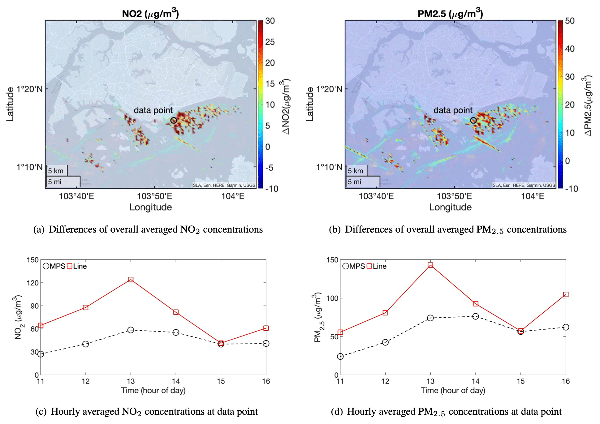
Figure 18 Emission concentrations during the entire simulation period predicted by the MPS and LS models. Note that in panels (a) and (b), the 2D plots show the differences of the overall averaged concentrations during the entire simulation period (6 h) predicted by using the LS and MPS models (differences = LS results − MPS results). In panels (c) and (d), the curves present the hourly averaged concentrations predicted by two models at the location of the data point shown in panels (a) and (b), where large differences exist.

The simulation results by using the LS model are also presented in Fig. 17. Compared to the measured data, the NO₂ and PM_2.5 concentrations predicted by the MPS and LS models are generally similar, while the MPS model shows slightly better NO₂ results at the observation station A, which is closer to the ships than other stations. Fig. 18 also presents the overall averaged emission concentrations during the entire simulation period predicted by the MPS and LS models, and it clearly shows that the emission concentrations predicted by the two models are quite different, especially at the locations close to the ships. The different results for the two models are mainly attributed to the different treatments for the moving ships. However, as the emissions are transported to the locations far away from the ships (such as at the stations A–D), the differences of the emission concentrations predicted by the two models become smaller, due to the emission deposition and dilution. Although it may be expected that with a large number of ships and for large distances from the sources the LS model and the new MPS model will give similar results, the MPS model is a more realistic representation of the source and allows for greater granulation of the emissions, allows for a swift response of the pollution dispersion model to any changes in the ship movement and is expected to be equally accurate across all scales. Based on the results in this section and the simplified study, it is found that differences between the LS and the MPS models are small when a large number of ships are moving in a constant manner in the location of interest; however, the new MPS model could capture the impact of changes in the ship's course on the emission dispersion and hence provide more options to the modeler.

4 Conclusions

In this paper, a MPS model was developed to simulate the emission generation and transport from the moving ships in pollutant dispersion simulations. For the dispersion modeling, the common assumption is to use a LS or a FPS model to treat the emissions generated by the moving ships. Both models cannot update the ship movements within a certain time period (usually an hour), which results in an unrealistic emission distribution. In the MPS model, the ship movement parameters, including speed and direction, are used to update the ship positions and then to estimate the emission dispersion at different simulation times. The new developed model was integrated into the city-scale chemistry transport model, EPISODE–CityChem, and then was evaluated by simulating the atmospheric dispersion of emission species emitted by the ships in the Singapore area.

The computational results by using the MPS model were first compared to those obtained from a LS model and a FPS model in simplified simulations. Under the simplified conditions with a limited number of ships, the results indicated that the new developed MPS model can simulate the ship movement and hence predicts more realistic instantaneous concentration profiles for the emission species (such as NO₂) generated by the moving ships. In comparison, the LS model assumes a continuous and constant emission rate along the entire ship route and then results in much different emission profiles and cannot reveal the instantaneous impact of ship movements on air quality in the coastal area. For the FPS model, separated plume segments were observed in the simulation. Clearly, it is unrealistic as the emission is continuously generated by the moving ships from different positions at different time, and a continuous emission distribution should be formed. The hourly averaged values were compared as well for all three models. The comparison shows that the averaged concentration profiles are similar but with local differences for the MPS and LS models, mainly caused by the different treatments for emission release by the two models although the positions of emission release cover the same ship routes. The FPS model again was proven to be an inappropriate assumption for treating the moving emission source.

In addition, a real case study was conducted as well to further evaluate the MPS model by simulating all ships around the Singapore area. Compared to the measured data, the MPS model was found to reasonably predict the emission concentrations at different observation stations located in Singapore, although gaps still exist due to the different setups and configurations between simulations and measurements. The LS model was compared in the study as well. The predicted emission concentrations by the MPS and LS models are quite different at the locations close to the ships, while these differences become smaller at the locations far away from the ships as the emission is diluted and deposited. Compared to the measured data, the MPS and LS models perform similarly, while a slightly better NO₂ result was found for the MPS model at observation station A, which is closer to the ships. The real case study together with the simplified study suggests that the MPS model is a more realistic representation of the emission source, and it allows for greater granulation of the emissions and a swift response of the pollution dispersion model to any changes in the ship movement, compared to the LS and FPS models. The MPS also has a great potential for a real-time simulation of the shipping emission dispersion, when used together with the automatic identification system (AIS) ship position data. Therefore, the MPS model should be a valuable alternative for the environmental society to evaluate the pollutant dispersion contributed from the moving ships.

Appendix A: Parameter study – time step

To further evaluate the MPS model, the time step is investigated. In the reference case (case 1), the calculated time step is 15.8 s, and in this parameter study, the time step is adjusted to two different values of 10 s (case S1) and 30 s (case S2) as shown in Table A1. All other conditions and model setups for all three cases are the same.

The instantaneous NO₂ profiles at ground level for two additional time step simulations are plotted in Fig. A1. Compared to the reference case (Fig. 8), it indicates that the NO₂ profiles at different simulation time are almost same for all three cases, although the local emission distributions and concentrations are slightly different.

In EPISODE–CityChem, parallel simulations of emission dispersion are conducted, with one Eulerian main grid (where $\text{d}z=\text{d}y=\mathrm{1}$ km) built up to model the time-dependent advection and diffusion of emission species in the 3D space. At the same time, the emissions emitted from each point source in the sub-grid modeling are treated as finite Gaussian plume segments generated in each time step. The plume size and movement (speed and direction) are estimated based on the local meteorological conditions (mainly temperature, wind speed and direction) of the Eulerian grid cell, where the plume stays. In next time step, the plume position is updated, and then its size and movement parameters are re-calculated based on the new meteorological conditions of the main grid cell, where the plume segment is transported. In addition, when the length scale of the segmented plume (σ_y or σ_z, which is highly affected by the meteorological conditions such as wind speed and temperature) reaches a pre-defined value (usually one-fourth of the Eulerian grid size), the plume mass is integrated into the main Eulerian grid cell where the segmented plume is located and then deleted from the sub-grid model.

Table A1 Setups of pollutant dispersion modeling for parameter study.

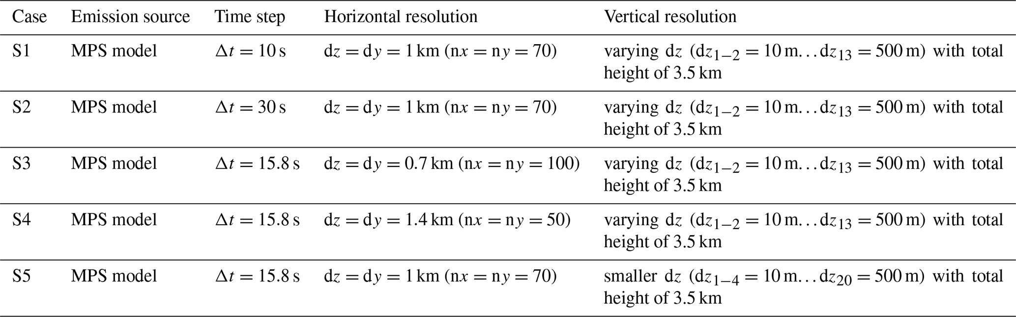
Figure A1 Instantaneous NO₂ concentrations near the ground by using different time steps. Top row: Δt=10 s (case S1); bottom row: Δt=30 s (case S2).

As the wind field (speed and direction) estimated by EPISODE–CityChem is spatially different (as shown in Fig. 4), the mass and number of plume segments and the values of other parameters (position, size, speed and direction) for each plume segment estimated in the dispersion modeling are different when using different time steps, and hence the plume prediction in the sub-grid modeling is different and results in different emission concentrations. However, as the time step reduces to a relatively small value, the impacts of time step on simulation results are negligible as shown in this paper (Figs. 8 and A1).

Appendix B: Parameter study – grid resolution

Another parameter study was conducted by changing the horizontal (case S3 and S4) and vertical (case S5) grid size. In this section, the dispersion of ship emissions was first simulated by using two different main grid resolutions, where the horizontal grid sizes (dz=dy) are changed to 700 m (case S3) and 1400 m (case S4), compared to the reference case (case 1, where $\text{d}z=\text{d}y=\mathrm{1}$ km). To keep the same simulation domain, the main grid has 100×100 cells in the horizontal direction for case S3 and 50×50 cells for case S4. All of other model setups (including vertical grid size and number) and initial conditions are the same for these cases.

The simulated NO₂ profiles for two additional grid resolutions are plotted in Fig. B1, which shows similar results to the reference case (Fig. 8) but with slightly different details. On the one hand, the space-varying wind fields for the different grid-resolution simulations are slightly different from the value in the reference case (case 1). As mentioned in the last section, the parameters of the plume segments, such as location, size and speed, are affected for the cases with different horizontal grid resolutions. On the other hand, the plume mass is added into the main grid cell where the plume is located, and then it induces a relatively higher local concentration for the finer grid and lower concentration for the coarse grid, compared to the reference case. Therefore, the integration of the sub-grid plume model with the main Eulerian model is affected and results in different NO₂ concentrations for the different grid setups. However, compared to the coarse grid (case S4), when the grid size is reduced, the simulation results for cases 1 and S3 are much closer to show mesh independence, as presented in Figs. 8 and B1.

Figure B1 Instantaneous NO₂ concentrations near the ground by using different grid resolutions. Top row: $\text{d}z=\text{d}y=\mathrm{700}$ m (case S3); middle row: $\text{d}z=\text{d}y=\mathrm{1400}$ m (case S4); bottom row: small dz (case S5).

A similar study was conducted by changing the vertical grid size (dz) as well. In this study, a smaller dz (especially at lower height) was applied in the simulation (case S5: 20 vertical layers), compared to the reference case (case 1: 13 vertical layers). All other setups and conditions are the same for the two cases. Similar conclusions are obtained in which the simulated NO₂ profiles are very similar, with only slightly different details for the two different setups, as shown in Figs. 8 and B1. The parameter study suggests that the MPS model works well for the shipping emission dispersion modeling.

Appendix C: Parameter study – emission source setup

In this study, the ship exit gas velocity was assumed to be 20 m s⁻¹ for all ships, and the chimney height was set as 30 m for large size ships and 10 m for small size ships (case 1). To investigate the effects of different setups for the MPS model on the simulation results, two additional cases were conducted by changing the exit gas velocity to 30 m s⁻¹ (case S6) and by increasing the chimney height to 40 m for all ships (case S7), as shown in Table C1. The comparisons of the simulated results obtained by using different setups are presented in Figs. 8a and C1. Based on the simulated NO₂ profiles, it can clearly be seen that the predicted results using different setups for the emission sources are almost identical, suggesting that the impact of different emission source parameters (such as chimney height and exit gas velocity) on the simulation results is quite small.

Table C1 Setups of emission sources for the MPS model in the parameter study.

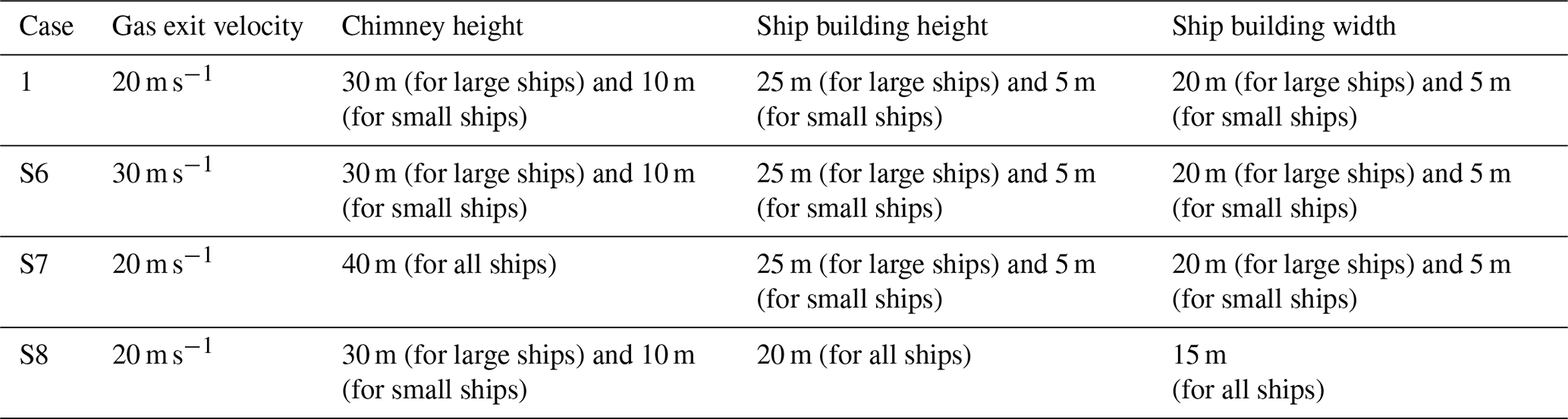
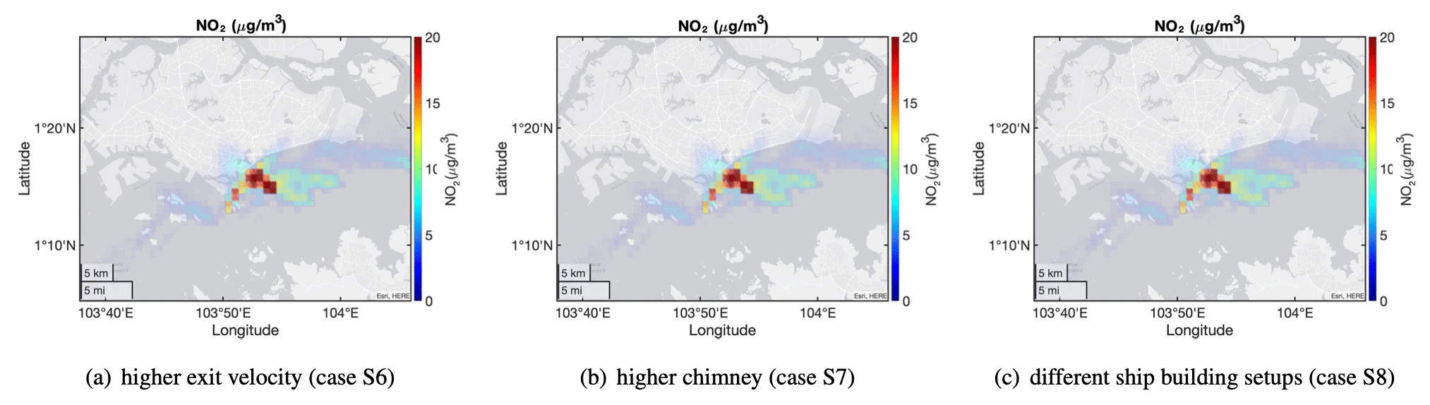
Figure C1 Instantaneous NO₂ concentrations near the ground by using different emission setups.

In addition, the ship building height was assumed to be 5 m below the chimney height, and the building width was set as 20 and 5 m for the large size and the small size ships respectively (case 1), as shown in Table C1. Another sensitivity study was conducted to evaluate the influences of different ship building dimensions on the simulation results, by assuming 20 m as the building height and 15 m as the building width for all ships (case S8). As shown in Fig. C1, the predicted NO₂ concentrations by using different ship building setups are very similar, compared to the reference results (case 1) in Fig. 8a. Therefore, this suggests that the impact of using these two different ship building setups on the simulations is negligible.

Appendix D: Results for different emission species

In this study, different species such as NO₂, SO₂ and PM_2.5 were simulated. However, the distributions of different species by using the same emission model (such as MPS model or LS model) are quite similar, and only the concentration values are different, as presented in Fig. D1. As the purpose of this paper is to demonstrate the development of the new MPS model and to show the differences of the simulated results by using the MPS model and other two common models (LS and FPS models), the paper only presents the predicted NO₂ profiles in the simplified study. In the real case study, the predicted NO₂ and PM_2.5 concentrations were presented to compare with the measured data in the observation stations, due to the data availability.

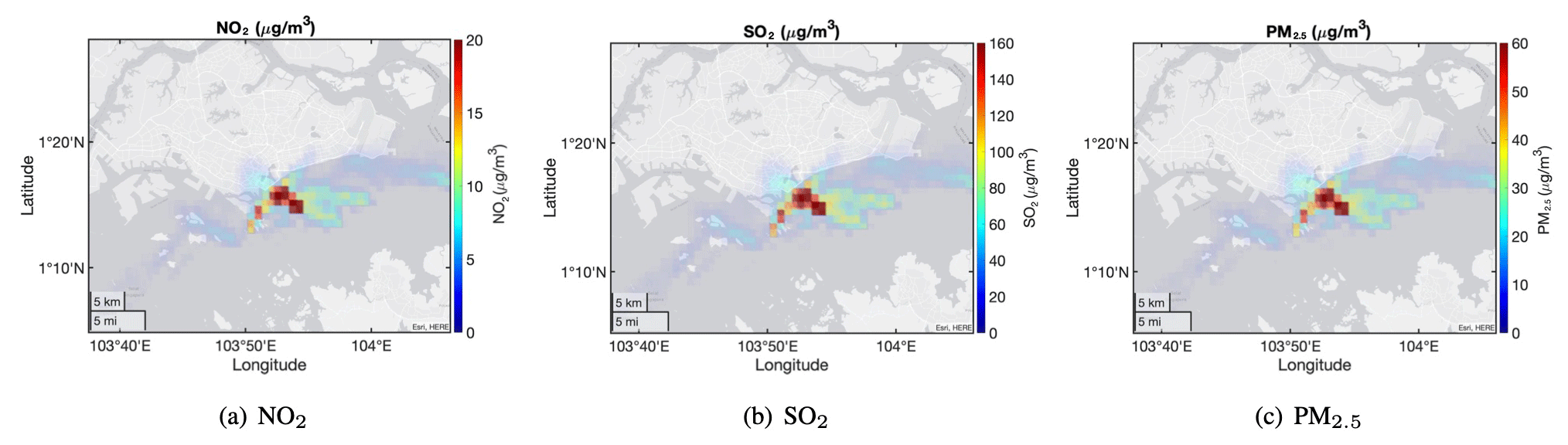
Figure D1 Predicted emission concentrations for different species when using the MPS model.