SCARLET-1.0: SpheriCal Approximation for viRtuaL aggrEgaTes

Aggregation of particles occurs in a large variety of settings and is therefore the focus of many disciplines, e.g., Earth and environmental sciences, astronomy, meteorology, pharmacy, and the food industry. In particular, in volcanology, ash aggregation deeply influences the sedimentation of volcanic particles in the atmosphere during and after a volcanic eruption, affecting the accuracy of model predictions and the evaluation of hazard and risk assessments. It is thus very important to provide an exhaustive description of the outcome of an aggregation process, starting from its basic geometrical features such as the position in space of its components and the overall porosity of the final object. Here we present SCARLET-1.0, a MATLAB package specifically created to provide a 3D virtual reconstruction for volcanic ash aggregates generated in central collision processes. In centrally oriented collisions, aggregates build up their own structure around the first particle (the core), acting as a seed. This is appropriate for aggregates generated in turbulent flows in which particles show different degrees of coupling with respect to the turbulent eddies. SCARLET-1.0 belongs to the class of sphere-composite algorithms, a family of algorithms that approximate 3D complex shapes in terms of a set of sphere-composite nonoverlapping spheres. The conversion of a 3D surface to its equivalent sphere-composite structure then allows for an analytical detection of the intersections between different objects that aggregate together. Thus, provided a list of colliding sizes and shapes, SCARLET-1.0 places each element in the vector around the core, minimizing the distances between their centers of mass. The user can play with different parameters that control the minimization process. Among them the most important ones are the cone of investigation (Ω), the number of rays per cone (N_r), and the number of orientations of the object (N_o). All the 3D shapes are described using the Standard Triangulation Language (STL) format, which is the current standard for 3D printing. This is one of the key features of SCARLET-1.0, which results in an unlimited range of applications of the package. The main outcome of the code is the virtual representation of the object, its size, porosity, density, and the associated STL file. In addition, the object can be potentially 3D printed. As an example, SCARLET-1.0 has been applied here to the investigation of ellipsoid–ellipsoid collisions and to a more specific analysis of volcanic ash aggregation. In the first application we show that the final porosity of two colliding ellipsoids is less than 20 % if flatness and elongation are greater than or equal to 0.5. Higher values of porosities (up to 40 %–50 %) can instead be found for ellipsoids with needle-like or extremely flat shapes. In the second application, we reconstruct the evolution in time of the porosity of two different aggregates characterized by different inner structures. We find that aggregates whose population of particles is characterized by a narrow distribution of sizes tend to rapidly reach a plateau in the porosity. In addition, to reproduce the observed densities, almost no compaction is necessary in SCARLET-1.0, which is a result that suggests how ash aggregates are not well described in terms of the maximum packing condition.

1 Introduction

The formation of aggregates from an initial set of individual monomers is a common topic in science, such as planetary formation, granulation processes, the food industry, meteorology, pollution, and Earth sciences (Brauer et al., 2001; Dominik et al., 2006; Poon et al., 2008; Brown et al., 2012; Cuq et al., 2013; Shi et al., 2015; Dacanal et al., 2016; Pumir and Wilkinson, 2016; Imaeda and Ebisuzaki, 2017; Ohno et al., 2020). In volcanology, aggregation plays a key role in affecting the sedimentation processes of ash in the atmosphere during and after a volcanic eruption, with deep consequences for the accuracy of the dispersal forecasting and hazard assessment (Durant, 2015).

The study of aggregation with experimental setups or direct observations in natural environments is often a challenging – if not impossible – task (Karrer et al., 2020). For this reason, the use of virtual reality has been considered a valuable alternative to direct investigation (Lumme and Rahola, 1994; Filippov et al., 2000; Min et al., 2007).

Several algorithms have been dedicated to the numerical solution of theoretical problems concerning aggregation phenomena, such as the study of the maximum packing of geometrical shapes within fixed boundary conditions (Conway and Sloane, 1998; Weaire and Aste, 2000; Williams and Jia, 2003; Donev et al., 2004; Hales, 2005; Man et al., 2005); other codes have been specifically written for the investigation of aggregation in natural contexts. Among them, we only mention algorithms aimed at studying aggregates in protoplanetary disks (Ormel et al., 2007; Yurkin and Hoekstra, 2011), ice formation and snowflake aggregation (Kessler et al., 1984; Westbrook et al., 2004; Maruyama and Fujiyoshi, 2005; Reiter, 2005; Ning and Reiter, 2007; Tyynela and von Lerber, 2019; Ori et al., 2014; Karrer et al., 2020), and in other environmental applications, such as water treatment (Chopard et al., 2006). Several codes treat aggregation as a fractal process such as in diffusion-limited aggregation (DLA), in which the characteristic length of the aggregate, R, can be related to the number of monomers involved, N_p, and the fractal dimension, D_f, by means of the power law $N_{\text{p}}\propto R^{D_{\text{f}}}$ (Nguyen et al., 2003, 2004; Jacobson, 2005).

Another important aspect concerning aggregation algorithms is the capability to accurately describe the shapes of the particles involved. In some circumstances the morphology of the colliding objects is sufficiently well described in terms of equivalent spheres. In other cases, a more accurate description is needed, for example in the study of particle packing (Man et al., 2005) or in all cases in which particle interlocking plays a key role, such as in snowflake formation.

In volcanology, despite the importance attributed to ash aggregation, no specific code has been designed so far for the study of particle packing geometries or, in general, the dependency of aggregate densities with respect to their structural configuration. Several types of different aggregate geometries have been described in literature, from particle clusters (PCs) to accretionary pellets (APs) (see Brown et al., 2012, for a complete review). In particular, recent field observations have revealed how PC3 objects have a key role in ash sedimentation (Bagheri et al., 2016; Gabellini et al., 2020). PC3 types are roughly spherically symmetrical in shape and are composed of big particles of about 200–1000 µm (the core) at the center of the structure, with many smaller particles (typically < 100 µm) around it (the coating).

The physical explanation for the formation of PC-type aggregates involves the theoretical description of a polydisperse particle population within a highly turbulent flow, as is the case for a volcanic plume or cloud (Kieffer and Sturtevant, 1984). In the presence of a cascade of turbulent eddies and grains of different sizes, particles will show different degrees of coupling with the turbulent flow (Volk et al., 1980). This will produce a wide spectrum of relative velocities (Ormel and Cuzzi, 2007). In the limiting case of particles with a negligible velocity correlation with respect to the others (i.e., the kinetic theory limit), the object will aggregate following an inertial aggregation mechanism (Textor and Ernst, 2004). This is typical of large particles that will cross from one eddy to another with a poor correlation with the dynamics of the eddies. In their path across the turbulent flow these objects will encounter smaller particles that, in contrast, do show a high correlation with the eddies. This process can be modeled as a central collisional process in which the big particle is the target of random collisions coming from random directions.

All these aspects motivated us to create SCARLET-1.0 (SpheriCal Approximation for viRtuaL aggrEgaTes), a MATLAB package designed for the study of volcanic ash aggregation generated by central collisional processes of particles with arbitrary 3D shapes. SCARLET-1.0 simulates the binary and sequential collision between the core and a vector of N_p particles. The algorithm follows a Monte Carlo approach to investigate the final positions of the ith particle and the already placed aggregate, minimizing the distance between the center of mass of the two bodies. Once the ith particle has been placed, it is considered fixed within the aggregate.

One of the main problems related to the aggregation of objects with complex surfaces is the detection of the intersections between them. SCARLET-1.0 belongs to the so-called sphere-composite algorithms (Evans and Ferrar, 1989; Nolan and Kavanagh, 1995), in which each single shape is seen as the superposition of N_sp nonoverlapping spheres. Describing a given shape in terms of a set of spheres leads to a pure analytical solution when searching for intersections between multiple shapes. On the other hand, a large number of spheres is required for collisions for which a high degree of accuracy is needed (Jia and Williams, 2001).

The most innovative aspect of SCARLET-1.0 is the use of the Standard Triangulation Language (STL) to describe the 3D shapes involved in the collisions. STL is currently one of the most common formats for 3D printing, 3D scanning, and design (Szilvasi-Nagy and Matyasi, 2003). This guarantees great flexibility to create virtual aggregates with SCARLET-1.0 starting from a set of completely arbitrary shapes. As a demonstration of this, in the main body of the paper and in the Appendix we show virtual aggregates made of a great variety of shapes: from scientific ones, such as volcanic particles, snowflakes, cones, ellipsoids, and spheres, to the most creative ones. It is important to demonstrate that SCARLET-1.0 also produces as output the STL file of the final aggregate: this means that the virtual aggregate can be potentially 3D printed. This makes an innovative link between simulations in the virtual reality and experiences in the real world, such as laboratory investigations of the drag force exerted on complex aggregates (McCorquodale and Westbrook, 2021).

The paper is structured as follows: in Sect. 2 we described the model, with a focus on the functions fromStlToSpheres and mainSCARLET. In Sect. 3.1 the algorithm is tested for aspects concerning the calculation of porosity problems. In Sect. 3.2 we present an application of SCARLET-1.0 to the study of both generic ellipsoids and the evolution in time of volcanic ash aggregates. In Sect. 4 a short discussion of the pros and cons of the package is presented.

2 Model description

2.1 Physical description of the aggregation process and model design

SCARLET-1.0 is written in MATLAB (tested for MATLAB R2015b), and it has been motivated by the need for a better understanding of the geometrical packing of volcanic ash aggregates observed during volcanic eruptions (Taddeucci et al., 2011; Brown et al., 2012; Bagheri et al., 2016; Gabellini et al., 2020). It simulates the random collisions encountered by the core in its path across an environment where N_p particles of arbitrary sizes and shapes are present. This happens in nature when particles with different dynamical properties are released in a turbulent flow. In this case the complex interaction of a cascade of turbulent eddies and the presence of particles with different sizes and masses produce a wide spectrum of particle Stokes numbers and thus a complete set of different degrees of coupling with the flow (Ormel and Cuzzi, 2007). The limiting cases for the situation under analysis are described in the literature as the Saffman–Turner limit (Saffman and Turner, 1956) for particles fully coupled with the fluid and with a size smaller than the Kolmogorov scale as well as the kinetic theory limit (Abrahamson, 1975; Textor and Ernst, 2004), in which large particles are poorly coupled with smaller eddies. The final result of the process is a population of large particles with uncorrelated relative velocities that are higher as the decoupling with the flow is more pronounced (Volk et al., 1980). This is, for example, what happens in the case of coarse ash within a turbulent volcanic plume or cloud (Textor and Ernst, 2004) and also for dust grains in protoplanetary disks (Ormel et al., 2007; Okuzumi et al., 2009). The presence of a relative velocity between the core (or the aggregate) and the colliding particle creates a relative kinetic energy that must be dissipated in order to have a successful sticking. In SCARLET-1.0 we do not focus on the dissipation mechanisms, which require a full understanding and constraint on nontrivial quantities such as the presence of viscoelastic forces, water layers, electrostatic charges, and plastic deformations. Since we are mostly interested in the final geometrical packing, we simply assume that after the collision the ith particle will dissipate the relative kinetic energy available and stick to the central structure.

In summary, within the limit of the kinetic theory limit the large core shows a negligible correlation with the velocity of the surrounding particles, and it acts as a central pole of accretion for the colliding particles in its path across the turbulent eddies if a Lagrangian perspective is assumed. Moreover, considering that the core can indeed rotate and that the turbulence is usually assumed to be isotropic in the theoretical descriptions (Volk et al., 1980), the angles of collisions with respect to the central body are assumed to occur at random orientations.

In SCARLET-1.0 we fix the system of reference (SOR) at the center of mass (CM) of the core in a purely Lagrangian description of the motion. The core, which is of arbitrary shape, is the target for the collisions and the population of particles encountered as the aggregation process evolves is defined as a vector of particles with different sizes and arbitrary shapes. According to the physical process that we want to describe, collisions happen at random angles around the central structure and the collision cone is centered in the CM of the core. This is the main mode of operation of the code and the motivation that led us to create it according to what has been recently observed in volcanic eruptions (Bagheri et., 2016; Gabellini et al., 2020). However, it is worth anticipating here that SCARLET-1.0 allows relaxing some of these constraints if needed by the user. For example, collisions can occur following a fixed direction of collision, and the collision cone can be centered in alternative locations with respect to the CM of the core.

The main steps with which the aggregation process is modeled in SCARLET-1.0 are summarized here.

1. Definition of the shapes involved in the aggregation process. Every different shape used in the simulation must be already present in the folder as an STL file. STL files can be generated by means of specific CAD software; they can be downloaded from the internet or simply obtained by 3D scanners. The use of binary STL files is preferred with respect to the ASCII format.

2. The sphere-composite representation of each STL file. SCARLET-1.0 uses a dedicated script named fromStlToSpheres to construct the sphere-composite representation of the original shape (see Sect. 2.1). STL files are defined by a set of points and facets. The script takes advantage of the MATLAB function inpolyhedron (Sven, 2021) to generate random points within the surface. Once the point is created within the STL shape and outside an already existing sphere, it generates a new sphere (see Sect. 2.2). Each single shape that the user wants to involve in the simulation must be pre-processed by fromStlToSpheres.

3. Generation of the monomer's distribution. The grain size distribution of the coating is defined a priori by the user, who defines a vector of particle sizes with a length equal to the number of particles involved (N_p). Each element of the vector indicates the maximum length $d_{\text{max}}^i$ of the ith particle (in arbitrary units). The shape attributed to the ith particle is randomly selected within those available for the coating (see Sect. 2.1). The core size $d_{\text{max}}^{\text{core}}$ is defined by the user and corresponds to its maximum length (in arbitrary units a.u.). The shape attributed to the core is by definition the first element of the structure generated by the pre-processing function fromStlToSpheres.

4. Selection of the particles that will collide. Particles are selected sequentially from the previously defined vector of sizes. Therefore, the contemporary deposition of two particles is forbidden (i.e., only binary collisions are treated).

5. Collision trajectory. In order to place the ith particle, a cone is generated with its center in the CM of the core (or, alternatively, in one of the spheres that form the sphere-composite representation of the aggregate). N_r random rays are uniformly generated within the cone, and the shape associated with the ith particle – scaled to its actual size – is randomly rotated N_o times along each ray, following the Z–X–Z convention on the Euler's angles. Each rotated object is by default placed outside the aggregate. Then a coarse inward movement along the ray is performed until the overlapping of the sphere-composite representations of the aggregate and the ith particle happens. At this stage a finer outward movement along the ray is done until there is overlap between the spheres. The two-step process guarantees faster movements when the objects are far away and a fine tuning when they overlap.

6. Contact dynamics. The contact dynamic assumes an instantaneous sticking when the intersection of the spheres is no longer present (see step 5). This means assuming that the relative kinetic energy is completely dissipated at the moment of impact, with no rearrangement of the already existing structure. For each ith particle a total of N_r×N_o configurations are tested but we only take the one that minimizes the distances between the CM of the aggregate and the particle. This is equivalent to assume that among the N_r×N_o configurations the inward force and the torque oriented the particle in such a way to minimize this distance.

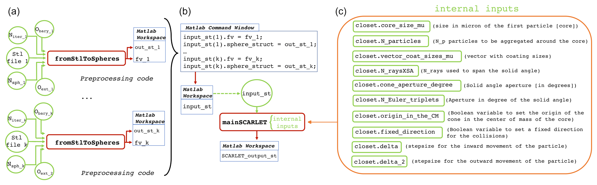
Figure 1 General scheme of SCARLET-1.0: (a) the pre-processing code fromStlToSpheres and (b, c) the main function mainSCARLET. The pre-processing code is needed to convert each 3D shape into a set of nonoverlapping spheres. The function fromStlToSpheres produces two output structures for each STL file, out_st and fv, which must be assembled into a new structure, input_st, as shown here; input_st represents the unique external input for mainSCARLET. A set of internal inputs control the details of each simulation, such as the number of coating particles involved, their sizes, and the degree of packing.

Figure 2 Example showing how SCARLET-1.0 creates a loosely packed aggregate made of 20 ellipsoids and cones of different sizes around a central object (a T-rex).

2.2 General overview of the code

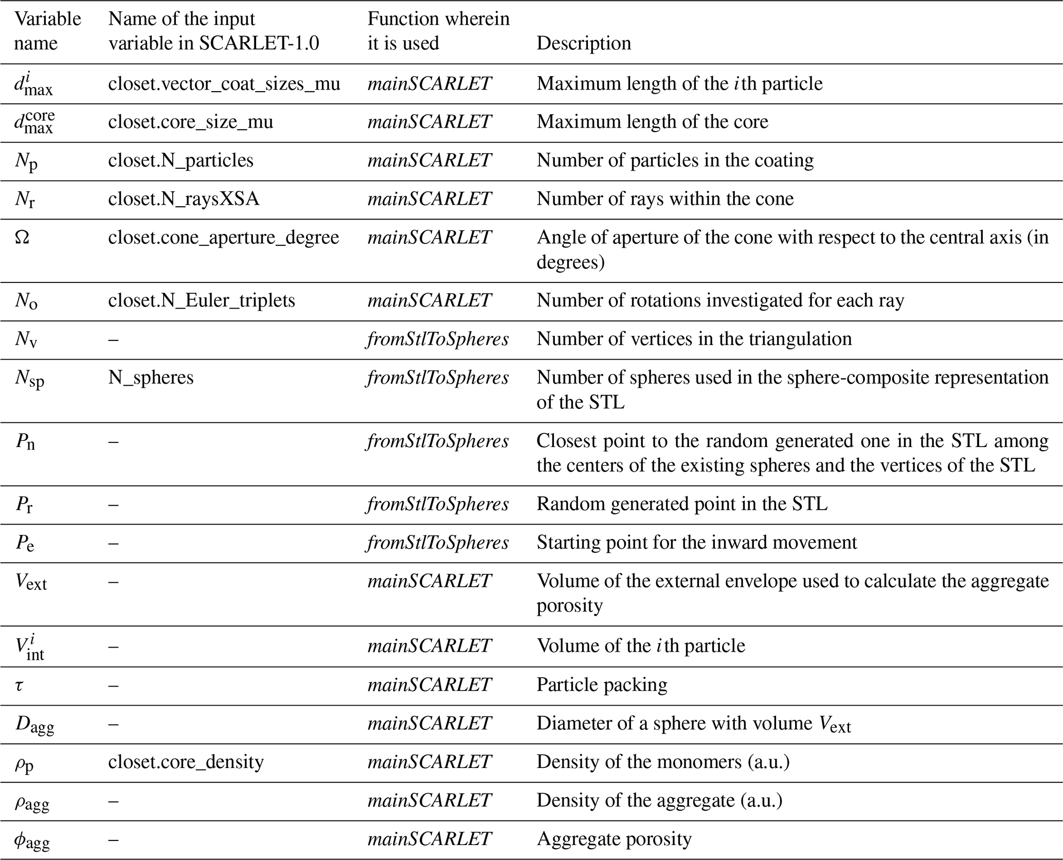
In the following we present a general description of the two main functions fromStlToSpheres and mainSCARLET, which are respectively responsible for creating the sphere-composite representation of the single shapes and building the virtual aggregate (Fig. 1). For further details on how to use the code we wish to direct the interested reader to the dedicated user guide at the GitHub link: https://github.com/EduardoRossiScience/SCARLET (last access: 14 July 2021) (and also at the Zenodo repository: https://doi.org/10.5281/zenodo.4675770, Rossi, 2021). In Table 3 we summarize the main parameters used in the code.

2.2.1 The pre-processing code fromStlToSpheres

The pre-processing code fromStlToSpheres translates a given 3D STL volume into a random set of nonoverlapping spheres. The STL standard describes any closed surface with a triangulation of vertices and faces. Vertices are expressed as a matrix with three columns and a number of rows equal to the number of vertices N_v. The N_v vertices are points distributed along the surface of the STL shape (Fig. 3a, d). Faces are instead described by a matrix of three columns and $\frac{N_{\text{v}}}{\mathrm{3}}$ rows; each row contains three integers reporting the corresponding vertices involved in the creation of the face.

The fromStlToSpheres function generates a random point P_r inside the 3D surface using the function inpolyhedron. This operation is repeated until P_r is generated outside an existing sphere. Then we find the closest point P_n among all the vertices of the triangles (see Fig. 3a, d) and the centers of already placed spheres. If P_n∈N_v, the radius of the new sphere is $\stackrel{\mathrm{‾}}{P_{\text{r}}{P}_{\text{n}}}$; in contrast, if P_n is one of the already placed spheres, the radius is $\stackrel{\mathrm{‾}}{P_{\text{r}}{P}_{\text{n}}}$ minus the radius of the sphere whose center is P_n. In conclusion, the newly placed sphere will be tangent to the STL surface or to another sphere.

In Fig. 3 fromStlToSpheres is applied to two different volcanic particles: Fig. 3a and d illustrate the vertices of the triangles of the STL volume. In Fig. 3b and e, both volcanic particles have been filled with N_sph=300 spheres. In Fig. 3c and f the reduction of the spheres is obtained by setting O_ext=1, a Boolean variable that allows eliminating the internal spheres.

Figure 4 shows some applications of the pre-processing routine to different shapes, each of them characterized by a different degree of complexity, such as convexity of the shape and volume. The scaling of the object produced by fromStlToSpheres is the same as the one contained in the original STL file (expressed in a.u.). No modification is done at this stage. The function mainSCARLET will rescale the core and the coating according to vector defined by the user (i.e., $d_{\text{max}}^{\text{core}}$ and $d_{\text{max}}^i$).

Figure 3 Application of the pre-processing routine fromStlToSpheres to two different volcanic particles. Blue points in (a) and (d) represent the vertices of the triangles used to define the 3D surfaces, as present in the original STL files. Panels (b) and (e) illustrate the final process of filling the volumes with 300 spheres placed randomly inside the objects. Panels (c) and (f) show the most external spheres obtained using the built-in MATLAB function boundary.

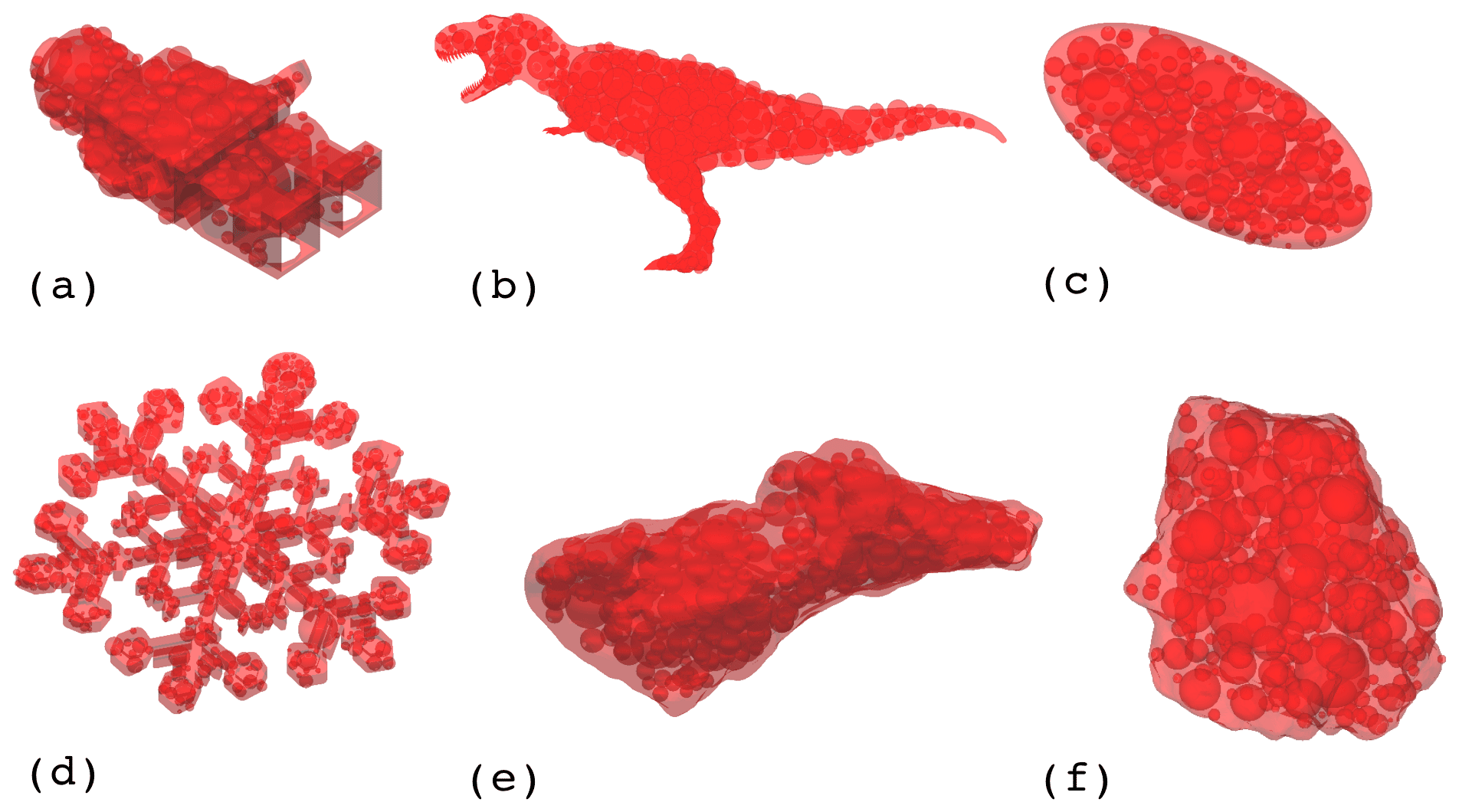
Figure 4 Application of the pre-processing routine fromStlToSpheres to objects characterized by different surfaces (i.e., convex hulls or not) that will be used in this paper: (a) a toy character, (b) a T-rex, (c) an ellipsoid, (d) a snowflake, and (e, f) two different volcanic particles. No scale has been reported for this image since it is not important for the pre-processing. In fact, all the objects will be rescaled by the main SCARLET function.

Figure 5 Scheme followed by SCARLET-1.0 for particle placing. (a) The first part of the algorithm whereby shapes are randomly assigned to each coating particle and scaled to the actual particle size is shown. (b) The series of five nested loops that control the particle placing is presented.

As an example, let us assume that we want to create a virtual aggregate made of three different shapes: a T-Rex shape for the core and a cone and an ellipse for the coating (see Fig. 2). The pre-processing code must be executed three times, one for each STL file. In the MATLAB command window we type the following.

[core_spheres, core_fv] = fromStlToSpheres(volcanic_particle.stl, 300, 3, 0, 1);
[coating1_spheres, coating1_fv] = fromStlToSpheres(ellipse.stl, 300, 3, 0, 1);
[coating2_spheres, coating2_fv] = fromStlToSpheres(cone.stl, 300, 3, 0,1);

Each time that fromStlToSpheres is executed two distinct structures are produced as output in the workspace. In core_spheres, coating1_spheres, and coating2_spheres, the information relative to the spheres is stored. In core_fv, coating1_fv, and coating2_fv, the information is relative to the triangulation of the STL surface (i.e., faces and the vertices). This operation needs to be done only once for each shape: all the structures can be saved for further simulations.

The input structure for mainSCARLET (input_ struct in the example) must be assembled at this stage by simply typing the following in the command window.

input_struct (1).fv = core_fv;
input_struct (1).sphere_struct = core_spheres;
input_struct (2).fv = coating1_fv;
input_struct (2).sphere_struct = coating1_spheres;
input_struct (3).fv = coating2_fv;
input_struct (3).sphere_struct = coating2_spheres;

The first element of input_struct will be assigned to the central core. The other shapes will be assigned randomly to the coating particles. The structure input_struct is the unique external input required by mainSCARLET that is now ready to be used.

2.2.2  mainSCARLET

The mainSCARLET function creates virtual aggregates from the available set of shapes contained in the input structure described in Sect. 2.2.1. It is composed of two distinct blocks (Fig. 5): the first one assigns a 3D shape to the ith object of the vector of N_p coating particles; then it scales the shape and the inner spheres in order to make the maximum size of the STL of the ith object equivalent to $d_{\text{max}}^i$. The second block places the ith object around the inner core, whose center of mass (CM) is coincident with the origin of the axes. The first shape of the input structure is assigned by default to the core, and it is scaled to have the maximum length of the STL equivalent to $d_{\text{max}}^{\text{core}}$.

The algorithm for particle placing is based on five main loops.

• Loop 1 (for i=1 to N_p). For each coating particle the code generates a cone of aperture Ω with respect to the unit vector $\widehat{\mathit{v}}$, which is randomly and uniformly oriented on the surface of a unitary sphere. The center of the cone can be placed at the CM of the core or at the center of one of the spheres of the sphere-composite representation of the aggregate, according to the user specifications. In the case of a central core whose CM is outside the STL file, the second option is activated by default. The angle Ω is measured in degrees with respect to the central axis of the cone (i.e., $\mathrm{\Omega }=\mathrm{0}{}^{\circ }$ coincides with $\widehat{\mathit{v}}$). Large values produce a wider exploration of the surface of the aggregate before placing the coating particle; in contrast, small values of Ω generally produce loose aggregates. The user can also fix a preferred direction for the cone for all cases in which collisions occur along a preferential direction. We will not make this assumption in the rest of the paper, assuming that the collisions described come from a fully isotropic turbulence with random angles of collisions.

• Loop 2 (for j=1 to N_r). N_r rays are generated within the ith cone. The code computes the most external intersection point P_e of each ray with the spheres already placed in the aggregate.

• Loop 3 (parallelized, for k=1 to N_o). The shape is randomly rotated N_o times in the space along three angles [φθψ], according to the Euler rotation matrix (Z–X–Z convention). This loop is parallelized using parfor.

• Loop 4. This loop moves the ith particle inwards starting from the position $P_{\text{e}}+\mathrm{1.1}\cdot D_i$ along the direction of the jth ray. It stops when at least one intersection is counted between the spheres of the coating particle and the aggregate. The inward motion is a coarse and fast displacement of the particle. The step-size of this movement is defined as a fraction f_c1 of the particle size (suggested values $f_{\text{c1}}=[\mathrm{0.01}-\mathrm{0.001}])$.

• Loop 5. This loop moves the particle outwards from the last location reached in loop 4. It stops when the intersection of the spheres belonging to the aggregate and the coating particle is empty. The step size f_c2 of the outward movement is finer than f_c1 (suggested values $f_{\text{c2}}=[\mathrm{0.01}-\mathrm{0.0005}])$.

Figure 6 (a) Definition of the cone of exploration. The Ω angle (degrees) is zero along the central axis of the cone. (b) Cone, rays, and rotations associated with the placing of one single coating particle. In the figure, the cone is coincident with the center of mass of the core. However, the user can modify the Boolean variable closet.origin_in_the_CM in order to make the center of the cone coincident with one of the spheres of the sphere-composite representation of the STL file.

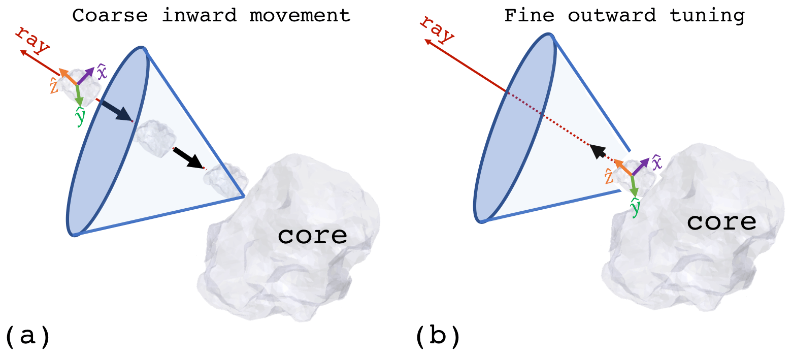
Figure 7 Coarse inward movement and fine outward tuning associated with loop 4 and loop 5, respectively.

For a given ray within the cone, SCARLET-1.0 determines the rotated particle that has the minimum distance between the CM of the coating particle and the aggregate (Fig. 8). Finally, it selects the coating particle that among all the rays has the minimum distance with respect to the CM of the aggregate. Therefore, the ith coating particle will be placed after two minimization processes: the first one over all the rotations per ray and the second one over all the rays.

The mainSCARLET function produces two types of outputs: (i) three figures respectively showing the 3D image of the final aggregate, the external volume V_ext used for the calculation of the porosity, and the points used to determine the external volume itself; and (ii) output structures that contain the mass, density, porosity, size, external volume, and sum of the inner volumes of its components $V_{\text{int}}^i$. Finally, mainSCARLET generates in the root folder the STL file of the aggregate structure.

The calculation of the aggregate porosity requires some additional clarification here because it can vary according to the definition of V_ext. In SCARLET-1.0 the determination of the aggregate porosity is done under the assumption that the V_ext is the convex hull formed by the outermost points of its sphere-composite representation. This choice is a compromise between what has been observed in nature for PC3 aggregates (Bagheri et al., 2016; Gabellini et al., 2020) and the aim of reduced complexity in the algorithm. All the $V_{\text{int}}^i$ values are directly calculated from the surface of the scaled STL shape using the divergence theorem (Suresh, 2021). A unique density ρ_p is assigned to the monomers. The particle packing τ is evaluated according to Eq. (1).

$$\begin{array}{}\text{(1)}& \mathit{\tau }={\displaystyle \frac{{\sum }_{i=\mathrm{1}}^{N_{\text{p}}+\mathrm{1}}{V}_{\text{int}}^i}{V_{\text{ext}}}}\end{array}$$

The aggregate porosity ϕ_agg and density ρ_agg can then be easily quantified as

$$\begin{array}{}\text{(2)}& {\displaystyle }& {\displaystyle }{\mathit{\varphi }}_{\text{agg}}=\mathrm{1}-\mathit{\tau },\text{(3)}& {\displaystyle }& {\displaystyle }{\mathit{\rho }}_{\text{agg}}={\mathit{\rho }}_{\text{p}}\cdot (\mathrm{1}-{\mathit{\varphi }}_{\text{agg}}).\end{array}$$

Finally, the characteristic size D_agg assigned to the aggregate is the sphere-equivalent diameter calculated as the diameter of a sphere with the same external volume of the aggregate (Eq. 4).

$$\begin{array}{}\text{(4)}& D_{\text{agg}}={\left({\displaystyle \frac{\mathrm{6}}{\mathit{\pi }}}\cdot V_{\text{ext}}\right)}^{\mathrm{1}/\mathrm{3}}\end{array}$$

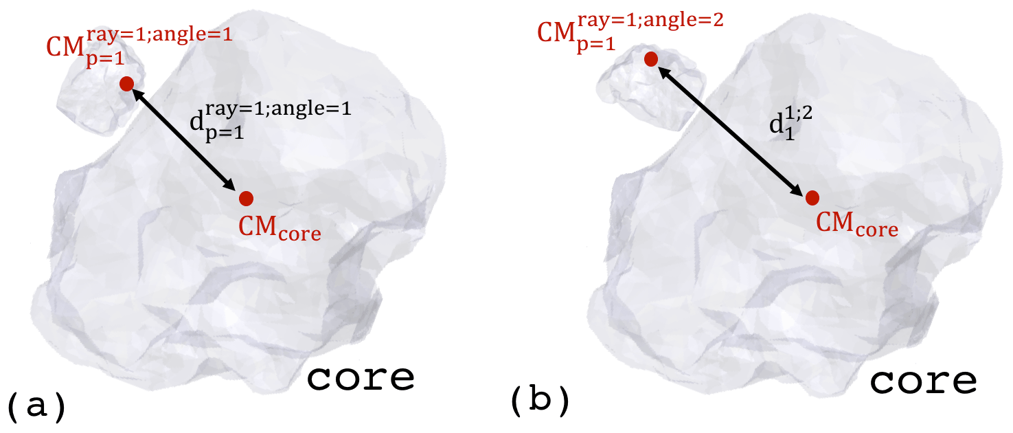
Figure 8 Example of the minimization process over two rotated particles. The selected particle is the one with minimum distance with respect to the center of mass of the core.

The algorithm takes advantage of the MATLAB built-in function convexHull, which is applied to the set of most external points among those describing the sphere-composition representation of the aggregate. Using points that belong to the sphere-composite representation instead of the STL file is a consequence of the need to increase the number of points generally used to define the external surface of objects involved in the aggregate. For a single STL characterized by a large number of facets and points, the use of a sphere-composite representation can lead to larger approximations in the determination of the porosity (or density). However, the code has not been designed for single particles, and the error gets relatively less important for aggregates. In fact, in these cases, what matters is how well the convex surface assumption describes the actual overall bulk volume of the object, more than the error in the single component. In any case, proper use of fromStlToSpheres is always preferred to obtain the desired sphere-composite representation of the irregular shape.

3 Results

3.1 Testing the model

3.1.1 Porosity evaluation using the convex-hull approximation: a comparison with analytical results

As outlined in Sect. 2, the porosity of an aggregate is always dependent on the surface that is used to define the external volume of the object. In SCARLET-1.0 the use of the convex-hull approximation is suitable for central collisional processes that result in roughly spherical aggregates, such as the PC1 and PC3 recently observed in the field (Bagheri et al., 2016; Gabellini et al., 2020). However, it can lead to an overestimation of the porosity for structures that are poorly approximated by a convex geometry, such as fractal-like aggregates. In all these cases the porosity should be considered as an upper-bound limit.

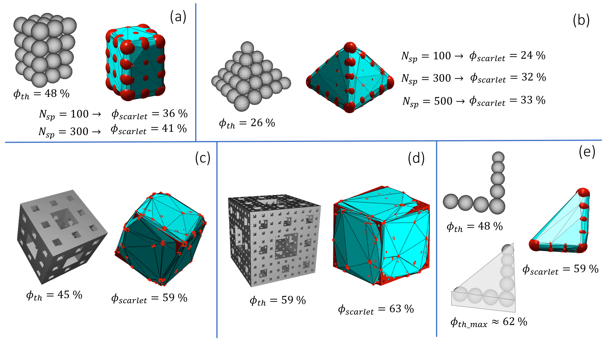
Figure 9 Evaluation of the accuracy in the determination of the porosity using the convex-hull surface of the most external points of the sphere-composite representation of structures for which the porosity is given. (a) Spheres packed with a theoretical 48 % porosity. (b) Spheres packed with a 26 % theoretical porosity. (c)–(d) Examples of Menger's sponge respectively obtained with two and three recursive processes. (e) L-shaped deposition of spheres for which the porosity is the same as in (a). The maximum theoretical porosity is evaluated considering the solid whose base is the L-shaped rectangular triangle and the height one sphere diameter.

In order to investigate the accuracy, we compared the porosity computed by the algorithm with those belonging to particular aggregate configurations or single objects for which analytical results are given in the literature. In Fig. 9a and b the comparison is made with respect to a classical configuration of sphere packing (e.g., the cannonball problem; Lucas, 1883). For these convex shapes the porosity difference is about 7 %–12 %, with a dependency on the number of inner spheres used to describe the shapes. In general, the higher the number of spheres, the higher the evaluated porosity. This is a consequence of a more accurate representation of the original structure. However, for a fixed number of spheres, the approximation is also dependent on how many points define the STL triangulation and from N_iter (i.e., how large the spheres are). In Fig.9c and d we calculate the porosity of the fractal shape known as “Menger's sponge”, respectively obtained with n=2 and n=3 recursive iterations with OpenSCAD (Hellweg et al., 2013), for which the porosity can be calculated as a function of the recursive step n (Sergeyev, 2009): ${\mathit{\varphi }}_{\text{n}}=\mathrm{1}-(\frac{\mathrm{20}}{\mathrm{27}}{)}^n$. For n=2 and n=3 the theoretical values are ϕ₂=45.1 % and ϕ₃=59.4 %. In our test we overestimated ϕ₂ and ϕ₃ by about 14 % and 4 %, respectively.

Lastly, Fig. 9e shows a non-convex L-shaped aggregate made of eight spheres. If the user-defined external volume is the one related to the void filling the space between two close spheres, this is equal to Fig. 9a (i.e., 48 %). In this case SCARLET-1.0 considers the convex surface that contains the spheres, which is close to the one defined by the triangular surface as the base and one sphere diameter as the height.

3.1.2 Porosity for aggregates made of spheres and ellipsoids and comparison with the maximum packing

Research on maximum packing has always shown an interest in mathematics and other practical applications (Hales, 2005; Man et al., 2005; Farr and Groot, 2009). As is evident from Eq. (1), porosity and packing are oppositely related: a larger packing will reduce the porosity of the aggregate and vice versa. Even if SCARLET-1.0 had not been specifically designed for research on maximum packing, it is somehow interesting to test the algorithm with respect to this branch of investigation, for which analytical limits are provided according to the shape of the single components under analysis. In this paragraph we will evaluate the packing τ of spheres and ellipsoids with principal axis ratios of a₁=1.25, a₂=1, and a₃=0.8, for which the theoretical values of the maximum packing τ are available in the literature (see Fig. 2 of Man et al., 2005). This particular choice of the principal axes constrains the value of flatness $f=\frac{a_{\mathrm{3}}}{a_{\mathrm{2}}}=\mathrm{0.8}$ and elongation $e=\frac{a_{\mathrm{2}}}{a_{\mathrm{1}}}=\mathrm{0.8}$. In our simulations we fix a₁=10 a.u. (arbitrary units), and we derive a₂ and a₃ from f and e (e.g., a₂=8 a.u. and a₃=6.4 a.u.). The average radius of the ellipsoid is defined as $\stackrel{\mathrm{‾}}{a}=(a_{\mathrm{1}}\cdot a_{\mathrm{2}}\cdot a_{\mathrm{3}}{)}^{\mathrm{1}/\mathrm{3}}$, and with R we indicate the radius of a sphere with the same external volume of the overall aggregate. The goal of the test is to relate the computed values of τ to the initial setup adopted in each simulation for solid angles, the number of rays, and the number of rotations, i.e., Ω, N_r, and N_o, respectively,. Virtual aggregates created in this test are made of identical particles with the same size. Packing is displayed in Fig. 10 as a function of the dimensionless parameter $\mathit{\gamma }=\frac{\stackrel{\mathrm{‾}}{a}}{R}$. A variable number of particles between a minimum of 10 and a maximum of 1000 has been used in all the simulations in order to achieve different values of γ.The results presented in Fig. 10 show that the condition of maximum packing for ellipsoids can be easily reached only for values of γ>0.3. For values of γ<0.3 a larger number of rays must be adopted to reach the same degree of packing. For spheres and for the conditions analyzed in this example, the maximum packing is reached for $\mathit{\gamma }>\mathrm{0.1}.$ As expected and clearly shown for spheres, the increase in the number of rays is not linearly related to the decrease in γ or to the increase in τ. In the search for the maximum packing, it seems that a large number of rays can have larger benefits with respect to the increase in the number of rotations, at least for the shape analyzed in this example. In addition, we notice that for spheres the minimum value for packing τ is about 20 %, a value that corresponds to a maximum porosity of 80 % (see Eq. 1). This threshold can be considered a good estimation of the maximum value for porosity reachable by means of the SCARLET-1.0 algorithm.

Figure 10 Packing τ of spheres and ellipsoids for different values of solid angles, numbers of rays, and numbers of rotations, i.e., N_r, Ω, and N_o, respectively. The red line indicates the maximum packing for ellipsoids with axes with a ratio of (1.25 : 1 : 0.8). The black line indicates the maximum theoretical packing for spheres. The number of monomers used in the test varied from 10 to 1000. Red dots are simulations made for ellipsoids, and black dots are for spheres. The red brackets show the values of N_r, Ω, and N_o used for a single simulation; the black brackets show the values of N_r and Ω, since no rotation of the shape is investigated for spheres. All the values are expressed as a function of $a/R$, where a is the average radius of the ellipsoid or sphere, and R is the radius of the sphere with same external volume of the aggregate.

3.2 Application of SCARLET-1.0 to packing problems

In this section two examples of possible applications of SCARLET-1.0 to different scientific problems are discussed. In the first example the attention is focused on the study of binary collisions of generic ellipsoids, i.e., aggregates made of just two particles. In particular, the goal here is to determine how the porosity of the final product depends on the flatness and elongation of the ellipsoids and their relative sizes. Ellipsoids are often used to approximate complex shapes; this application is thus of general interest for different scientific topics, such as particle sedimentation and particulate transport. In the second example, SCARLET-1.0 is instead applied to the investigation of how the porosity evolves in time for volcanic ash aggregates. In this application, parameters of real volcanic aggregates are used to constrain the free parameters of the algorithm (Ω, N_r, N_o) and to draw important conclusions on the evolution of these objects.

3.2.1 Porosity for particle–particle collision of two generic ellipsoids

A collision of two distinct bodies is always the initial seed for binary aggregation processes (Jacobson, 2005). The aggregate will then evolve in time, building up its own structure collision after collision and particle by particle. It is thus worth understanding the details of this initial stage, especially concerning how the 3D space is respectively filled by matter and voids. SCARLET-1.0 can be easily adapted to this problem, and an arbitrary number of colliding shapes can be investigated in theory. However, in this section we limit our attention to particle–particle collisions of ellipsoids due to their vast application in science as an approximation of much more irregular shapes (Bagheri et al., 2015). In this application we are interested in studying how the porosity ϕ_agg changes as a function of particle size ratios and their orientation in space. Here, as in the rest of the paper, the external volume for the calculation of ϕ_agg is defined by the convex-hull surface that bounds the two ellipsoids involved in the collision (Fig. 11b, c). This is equivalent to studying the maximum porosity that can exist between two single and non-vesiculated ellipsoids.

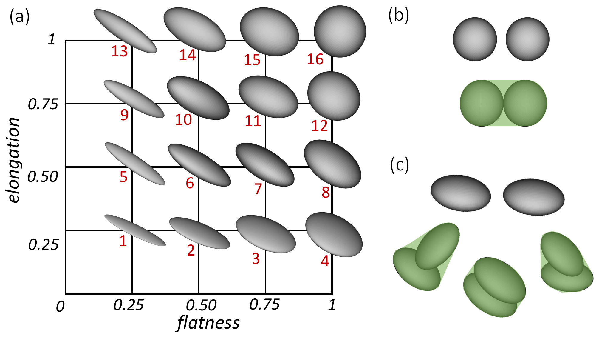
Figure 11 (a) The flatness elongation plane (FE plane) and the associated shape of the investigated ellipsoid. The red labels in the figure are introduced to characterize each particle–particle collision univocally. Panels (b) and (c) show some examples of how the external volume is defined in this application (i.e., the convex-hull volume that contains the two objects).

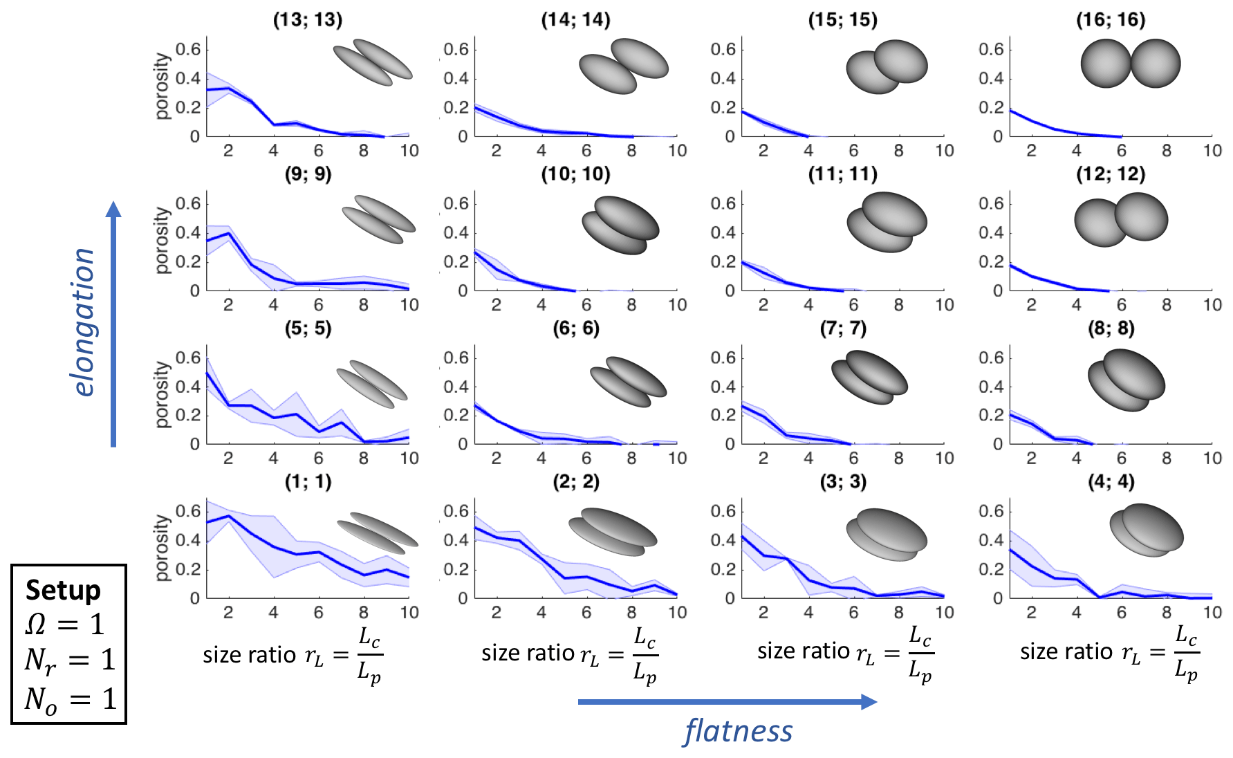
Figure 12 Porosity of two colliding ellipsoids of the same shape as a function of the size ratio r_L. The setup used in SCARLET-1.0 for these simulations is $\mathrm{\Omega }=\mathrm{1}{}^{\circ }$, N_r=1, and N_o=1. The pairs of numbers in the brackets refer to the shapes labeled in Fig. 10 The shaded area is the outcome of five simulations.

An ellipsoid is fully characterized by the knowledge of its three principal axes L, I, and S (where $L\ge I\ge S$). Here we describe the intermediate and smallest axes, I and S, respectively, in terms of flatness f and elongation e ($I=L\cdot e$ and $S=L\cdot e\cdot f$). This formalism allows describing the shape of any given ellipsoid as a single point in the flatness elongation plane (FE plane), as shown in Fig. 11, where 16 different ellipsoids have been created with OpenSCAD (https://www.openscad.org/, last access: 14 July 2021) to map the FE plane. When two ellipsoids collide, the resulting porosity ϕ_agg is also affected by the relative dimensions of the two objects, i.e., the size ratio r_L, described here in terms of the ratio between the major principal axes $\left(r_L=\frac{L_{\text{c}}}{L_{\text{p}}}\right)$, where the subscripts “c” and “p” indicate the central object and the colliding particle, respectively. It is worth noting that in general r_L is related to the ratio of the equivalent diameters $d_{\text{eq}}=(LIS{)}^{\mathrm{1}/\mathrm{3}}$ as follows: $r_{\text{d}}=\frac{d_{\text{c,eq}}}{d_{\text{p,eq}}}=r_L\cdot {\left(\frac{e_{\text{c}}^{\mathrm{2}}{f}_{\text{c}}}{e_{\text{p}}^{\mathrm{2}}{f}_{\text{p}}}\right)}^{\mathrm{1}/\mathrm{3}}$, which simplifies to r_d=r_L in the case of particles with the same flatness and elongation.

Figure 13 Porosity of two colliding ellipsoids of the same shape as a function of the size ratio r_L. The setup used in SCARLET-1.0 for these simulations is $\mathrm{\Omega }=\mathrm{90}{}^{\circ }$, N_r=30, and N_o=10. The pairs of numbers in the brackets refer to the shapes labeled in Fig. 10. The shaded area is the outcome of five simulations.

In this section we limit our attention to collisions of ellipsoids with the same shape but different size ratios r_L. Two different packings have been investigated five times: a loose packing (setup 1), for which $\mathrm{\Omega }=\mathrm{1}{}^{\circ }$, N_r=1, and N_o=1 (Fig. 12); and a much denser packing (setup 2), for which $\mathrm{\Omega }=\mathrm{90}{}^{\circ }$, N_r=30, and N_o=10 (Fig. 13). In Figs. 12 and 13 the pairs of numbers in brackets refer to the red labels in Fig. 11, which are used to identify the shapes involved in the collisions.

A few comments can be made on the results reported in Figs. 12 and 13. Firstly, the loose packing generally shows significantly more variability than the dense one (shaded areas in the figures), as is expected given that setup 1 completely depends on the initial random orientations of the bodies and the initial direction of collisions. Increasing the size ratios of the two objects or reaching the limiting case of a sphere (f→1, e→1), the variability goes to zero. Secondly, we notice that for collisions of particles of the same size ratio, where f≥0.5 and e≥0.5, the final porosity of the aggregate approaches ϕ_agg≈20 %, which corresponds to the analytical solution of two contacting spheres of the same size (as also confirmed by the simulations (16;16)).

Interestingly, if the shape of the objects is not characterized by extremely low values of elongation or flatness (e.g., less than 0.5), the threshold of 20 % represents a maximum value for porosities regardless of the size ratios involved in the collision, as clearly shown in Figs. 12 and 13. Scenarios become more complicated if flatness or elongation (or both) is less than 0.5 (i.e., needle-like or extremely flat objects): in all these cases we notice a dependence from the initial setups used in SCARLET-1.0 and, in general, higher values of the porosities with respect to the previous cases. As an example, for shapes labeled as (1;1) and r_L=1, setup 1 gives a porosity of ${\mathit{\varphi }}_{\text{agg}}=\mathrm{0.52}\pm \mathrm{0.13}$ compared to ${\mathit{\varphi }}_{\text{agg}}=\mathrm{0.42}\pm \mathrm{0.09}$ of setup 2. This last value is consistent with ${\mathit{\varphi }}_{\text{agg}}=\mathrm{0.44}\pm \mathrm{0.08}$ obtained by averaging 30 runs with the setup $\mathrm{\Omega }=\mathrm{90}{}^{\circ }$, N_r=60, and N_o=30.

3.2.2 Porosity of volcanic ash aggregates as a function of the aggregation stage

The term volcanic ash aggregation refers to the formation in the atmosphere or within a volcanic plume or cloud of agglomerates from tens of micrometers to a few millimeters in size due to the collision of smaller particles with a diameter generally less than 100 µm (Brown et al., 2012). As recently observed during the 2010 Eyjafjallajökull eruption (Iceland), volcanic ash aggregation plays a major role in ash sedimentation, as it affects the particle residence time in the atmosphere and potentially leads to an overestimation of ash concentrations in the atmosphere if it is underestimated in forecast models (e.g., Bonadonna et al., 2011; Durant, 2015). Unfortunately, despite its importance, many questions still remain open due to the complexity of the processes involved (Durant, 2015). A key factor is, for example, the porosity of volcanic ash aggregates, which strongly affects the sedimentation process and the residence time in the atmosphere. This parameter can be derived from field observations of the terminal velocity of the object before impact on the ground. However, field observations are difficult to obtain, and, in any case, they can only provide the porosity of the final structure of the aggregate, with no information about its evolution in time. In this section we apply SCARLET-1.0 to study the porosity evolution of volcanic ash aggregates, expressed as a function of the time, shapes, and grain size distributions involved in the process.

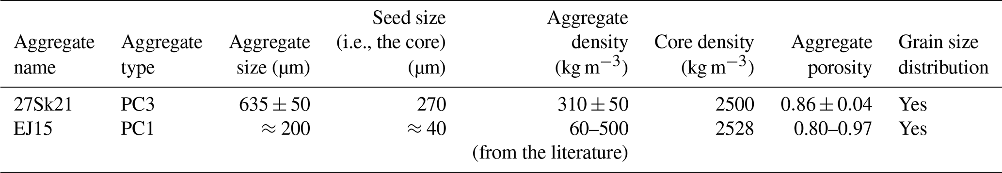
Here we apply our algorithm to the reconstruction of two specific aggregates associated with two different eruptions: the sample labeled as 27Sk21 belongs to the eruption that occurred on 3 August 2013 at Sakurajima volcano (Japan) (Bagheri et al., 2016); the sample EJ15 belongs to the eruption that occurred on 5 May 2010 at Eyjafjallajökull volcano (Iceland) (Bonadonna et al., 2011). Sample 27Sk21 was observed with a high-speed camera and was collected on an adhesive tape later analyzed with a scanning electron microscope (SEM); as a result, size and density could be derived before the impact on the adhesive tape from high-speed videos, while the grain size distribution could be derived from image analysis of the material collected on the adhesive tape (Bagheri et al., 2016). On the other hand, no high-speed video is available for aggregate EJ15; as a result, only the grain size distribution and a rough estimation of its size (about 200 µm) could be derived from the material left on the adhesive tape (Bonadonna et al., 2011).

The aggregates 27Sk21 and EJ15 were characterized as a cored cluster (i.e., Particle Cluster 3 – PC3) and ash cluster (i.e., Particle Cluster 1 – PC1), respectively (Bagheri et al., 2016; Bonadonna et al., 2011). PC1 represents clusters of ash particles with roughly all the same sizes of about 20–50 µm (Brown et al., 2012), whereas PC3 types are characterized by the presence of an inner single object larger than 200 µm that has been coated by hundreds of smaller ash particles (Bagheri et al., 2016).

Table 1 Observed features for aggregates 27Sk21 (Sakurajima, Japan) and EJ15 (Eyjafjallajökull, Iceland). For the 27Sk21 sample, aggregate and core size are observed from high-speed video; the aggregate density is derived based on settling velocity and size from high-speed video. Aggregate porosity is estimated based on measured particle density and derived aggregate density; core density is measured with a water pycnometer, and grain size distribution is derived from analysis of SEM images (Bagheri et al., 2016). For sample EJ15, the aggregate size, core size, and grain size distributions are derived from analysis of SEM images (Bonadonna et al., 2011), while the aggregate density and porosity are assumed based on the literature (Brown et al., 2012; Gabellini et al., 2020), and the core density is estimated based on a combination of a helium pycnometer and a theoretical relation with size (the reported value is the average for sizes less than 40 µm; Bonadonna et al., 2011).

SCARLET-1.0 requires a vector of sizes as an input to locate the coating particles around the core, i.e., the detailed grain size distribution forming the aggregate to be reconstructed. However, large uncertainties are expected to affect the measured grain size distribution due to (i) the mass lost in the air after the impact of the aggregate with the adhesive tape, (ii) the mass lost during the transport of the samples from the field location to the laboratory, and (iii) the overlapping of particles in the SEM images of the coating, which lead to a loss of information derived from the 2D representation of a 3D structure.

For aggregate 27Sk21, for which a constraint on size and density is available from the high-speed video, we make the assumption that all the losses in material only affect the total mass contained in the original coating population, but not the relative proportion of particles in each size bin. This is equivalent to considering the measured grain size distribution as fully equivalent to the original one, normalized for an unknown constant. The normalization constant is then derived by matching the size and density of the virtual aggregate to those derived from field observations.

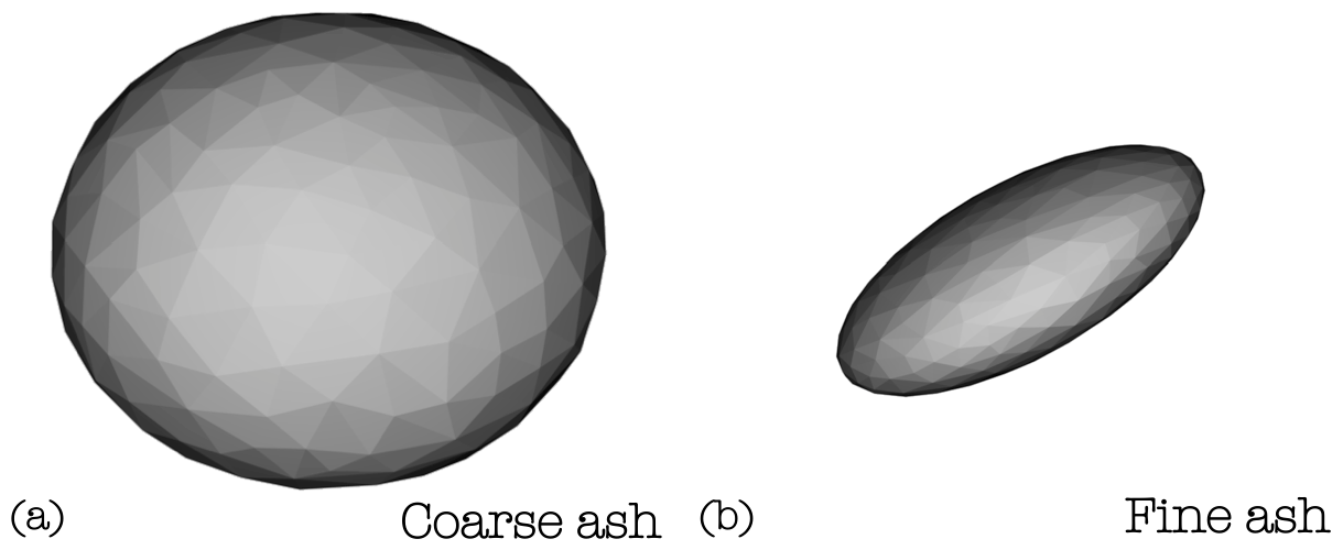
Figure 14 Ellipsoids used to characterize coarse (a) and fine (b) ash in the virtual reconstructions.

Volcanic ash particles are characterized by a variety of irregular shapes for which the STL representation of the surfaces is usually not available (an example of an aggregate made of real 3D scanned volcanic particles is presented in Fig. A1 of the Appendix). Here, in the absence of the actual shape of the single particles in the coating, we decided to approximate particles as ellipsoids. This choice is related to the observation that the drag of irregular particles can be sufficiently well described in terms of equivalent ellipsoids (Bagheri and Bonadonna, 2016). Moreover, we follow the simplified approach of classifying the coating population as two distinct classes, i.e., coarse (between 63 and 2000 µm) and fine (≤ 63 µm) ash, each of them characterized by a single specific ellipsoid as displayed in Fig. 14.

The two ellipsoids for coarse and fine ash are defined in terms of the three principal axes, derived by averaging the L, I, and S values of particles with sizes ≤ 63 µm and between 63 and 2000 µm from ash samples from the 2010 Eyjafjallajökull volcano (Iceland) (Table 2). These ellipsoids are used here to represent coarse and fine ash for both samples EJ15 and 27sk21. The actual size of the ith particle, $d_{\text{eq}}^i=(L_i{I}_i{S}_i{)}^{\mathrm{1}/\mathrm{3}}$, is used to scale the STL shape and to calculate the maximum length of the ith ellipsoid $L=\mathit{\alpha }\mathit{\beta }{d}_{\text{eq}}^i$ (where $\mathit{\alpha }=L/I$ and $\mathit{\beta }=L/S$) as required by SCARLET-1.0 (see Sect. 2.3).

Table 2 Geometrical features of the ellipsoids used to simulate fine and coarse ash. L, I, and S are the average of 2010 Eyjafjallajökull (Iceland) samples for particles with sizes ≤ 63 µm (fine ash) and between 63 and 2000 µm (coarse ash).

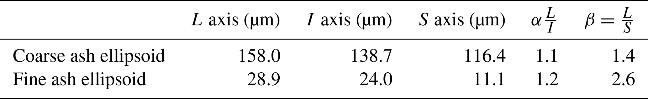
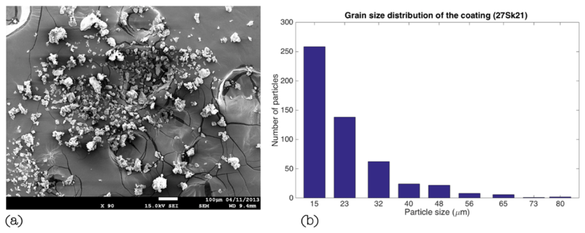
Figure 15 (a) SEM image of the coating particles relative to the aggregate 27sk21 (the big core escaped from the tape). (b) Grain size distribution derived from the SEM image (Bagheri et al., 2016). In the present work we did not use particles below 32 µm in size; this allows optimizing the computational efficiency without affecting the final result (since the volume scales as the third power of diameter, smaller particles add second-order contributions to the final volume).

In this virtual reconstruction we aim to reproduce the observed diameter of the aggregate (675 µm) and its final density (310 kg m⁻³) (Table 1) under the assumption that the measured grain size in Fig. 15b can be replicated N_A times in order to compensate for the expected mass loss. Single particles are assumed to have a density of 2500 kg m⁻³ (Bagheri et al., 2016). In our reconstruction particles below 32 µm in size are not taken into account in order to optimize the computational efficiency without affecting the final result. As a matter of fact, given that the volume scales as the third power of diameter, smaller particles add second-order contributions to the final packing. Several combinations of the solid angle Ω, number of rays N_r, and number of Euler rotations N_o have been tested. However, only a loose packing (e.g., $\mathrm{\Omega }=\mathrm{1}{}^{\circ }$, N_r=1, N_o≤5) and N_A=6 can approximately reproduce the observed features, which are characterized by a porosity larger than 80 % and an aggregate-to-core ratio of ≈3 (see Table 1). In Fig. 16 the variation of aggregate porosity is displayed as a function of collisions for four different scenarios: ellipsoids whose sizes are randomly picked from the grain size distribution (i.e., random displacement; blue line), ellipsoids sequentially located from the largest size to the smallest one (i.e., sequential displacement; red line), spheres whose sizes are randomly picked from the grain size distribution (black line), and spheres sequentially located from the largest size to the smallest one (i.e., sequential displacement; green line). Each line is the average of five repetitions, and the final size of the virtual aggregate is ≈ 600 µm.

The second object to be reconstructed is the PC1 aggregate EJ15, which was collected on an adhesive tape during the 2010 Eyjafjallajökull eruption (Iceland) (Bonadonna et al., 2011). The reconstruction is strongly affected by the lack of high-speed video, which does not allow us to characterize the aggregate size and density before impact with the adhesive paper. Therefore, in this application we simply focus on the time evolution of the porosity for different configurations of Ω, N_r, and N_o, keeping the grain size distribution equivalent to the one observed by Bonadonna et al. (2011) (i.e., no assumption has been made on the mass loss). In addition, the same ellipsoids reported in Table 2 have also been used for this application. The results of different simulations are reported in Fig. 17, together with the 3D visualization provided by SCARLET-1.0. In the following we refer to the setup with $\mathrm{\Omega }=\mathrm{50}{}^{\circ }$, N_r=30, and N_o=10 as “tight packing” and to the setup with $\mathrm{\Omega }=\mathrm{1}{}^{\circ }$, N_r=1, and N_o=1 as “loose packing”.

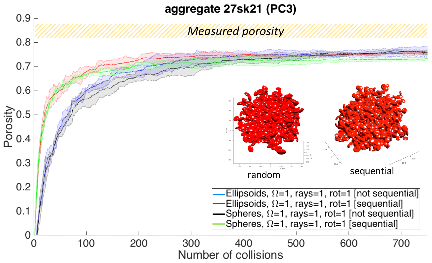
Figure 16 Evolution in time of the porosity for the aggregate 27Sk21, classified as PC3 from field observations and high-speed videos (Bagheri et al., 2016). The final reconstruction of the aggregate is reported in red within the frame of the figure for both a sequential and a random displacement of the coating particles. The core size – not visible in the figure – is 270 µm wide. The final size of the object matches the observed one (≈ 670 µm). The shaded area represents 68 % confidence around the mean over five repetitions. The angle Ω is expressed in degrees.

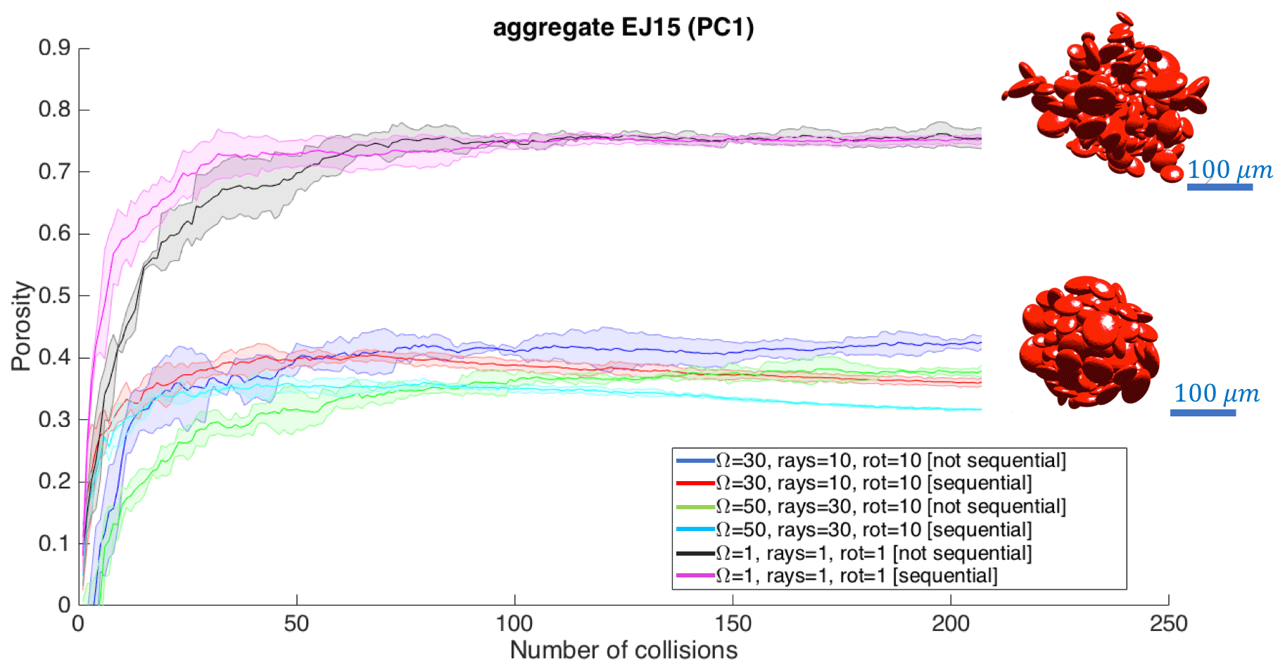
Figure 17 Time evolution of the porosity for aggregate EJ15 (PC1), collected during the 2010 Eyjafjallajökull eruption (Iceland) (Bonadonna et al., 2011). The virtual reconstructions are based on the same ellipsoids in Fig. 13. The shaded areas represent 68 % confidence around the mean over five repetitions. The angle Ω is expressed in degrees.

The range of final porosities spans from a maximum value of about 73 %–76 % for the loosest packing down to 30 % for the tight packing with $\mathrm{\Omega }=\mathrm{50}{}^{\circ }$, N_r=30, and N_o=10. If we compare the curves in Fig. 17 with values of porosities reported in the literature for PC1 aggregates of ≈ 80 %–97 % (Brown et al., 2012; Gabellini et al., 2020; Table 1), we can deduce that only the loose packing can realistically reproduce the observed features; such is the case for the PC3 aggregate.

Finally, it is important to notice how the plateau in porosity for EJ15 is reached roughly after the same number of collisions (≈ 50–70 collisions) for both the tight and loose packing.

4 Discussion

4.1 SCARLET-1.0: general comments on the operational use

SCARLET-1.0 has been specifically designed for the simulation of aggregation of complex shapes. In order to treat the intersection problem between colliding objects, the algorithm takes advantage of the sphere-composite representation of a body. This means that if a given shape is described in terms of N_sp spheres and if N_p particles collide, the final aggregate will be described as N_sp×N_p spheres. Given that the intersection is evaluated for each step in the inward and outward movement before placing each single particle (see Fig. 5), the use of a large number of spheres combined with a large number of particles can significantly increase the computational time of the package. As general advice, we recommend appropriate use of the pre-processing code fromStlToSpheres and the Boolean variable O_ext to find a good balance between an accurate description of the shape and a reduced number of spheres, i.e., faster computational times.

An important point that the user should always consider is how the parallelization of the algorithm works. The parallelization of the code is based on the execution of simultaneous for-loop iterations on the different available threads using parfor. However, MATLAB does not allow for nested parallel loops, which results in a parallelization that can only be performed at one level. As shown in Fig. 5, in the present release of SCARLET-1.0 this occurs inside the loop dedicated to describing particle rotations along a single ray. This means that if few rotations are set in the simulation the parallelization will not substantially speed up the code.

As outlined in the Introduction, SCARLET-1.0 has been created to simulate central collisional processes, in which particles collide from random directions and find their final location after spanning a given solid angle Ω. This occurs in different natural phenomena than the ones discussed in the previous examples and in the Introduction. According to the setup imposed by the external user, the package can simulate various degrees of packing by simply changing the solid angle of investigation (Ω), the number of rays (N_r), and the number of rotations (N_o). Concerning the maximum packing, Fig. 10 shows that objects characterized by a particle-to-aggregate size smaller than 0.17–0.25 require more computational efforts to match the maximum packing condition than aggregates with smaller sizes or larger components (at least for the shapes investigated). In these cases, the use of multiple processors allows having a large number of rotations tested, which can finally result in a better packing of the object in a lower computational time. However, in several applications of interest, such as the one reported in Sect. 3.2.2, the maximum packing is not the final aim of the virtual reconstruction and a much less dense packing is required to correctly mimic the phenomenon under analysis.

4.2 SCARLET-1.0 applied to the study of porosity for volcanic ash aggregates

In Sect. 3.2.2 we presented SCARLET-1.0 applied to the study of porosity in volcanic ash aggregates. This is an interesting example of how the algorithm can provide answers not only about the packing of shapes but also on its evolution in time, which is information that is usually missing in field or lab observations. The study has been focused on the virtual reconstruction of two specific aggregate structures: PC3 type (aggregate 27sk21), made of a central object 5 to 10 times larger than the particle sizes present in the coating; and PC1 type (aggregate EJ15), made of particles with roughly the same size.

The reconstruction of the PC3 aggregate (Fig. 16) has shown that the modeled aggregate porosity (≈ 73 %) is almost 10 % smaller than the observed one for the same size of the aggregate. This discrepancy can be due to the approximations made in the description of particle shapes. An alternative explanation can suggest the presence of liquid bridges in the original structure that alter the contact condition between particles and finally creates a looser packing of the coating (Gilbert and Lane, 1994). The setup used in the simulation that corresponds to loose packing (e.g., $\mathrm{\Omega }=\mathrm{1}{}^{\circ }$, N_r=1, N_o≤5) describes a particle coming from a random direction that is randomly oriented and is going to be located on the surface of the core immediately after the first contact. In this configuration no minimization is done on the packing of the aggregate and it should thus reproduce a condition of maximum porosity for the object. However, the fact that the observed porosity is even larger than the simulated one could be interpreted as a violation of the contact condition among particles as assumed by SCARLET-1.0. This violation is theoretically possible if liquid bonds act as a sticking medium between particles.

The importance of loose packing for the typologies under analysis is also confirmed by the PC1 sample (EJ15), for which the computed porosity of 73 %–76 % for the loosest configuration matches the lower bound of porosity reported in the literature (e.g., 80 %). This work thus suggests that the condition of maximum packing should not be seen as the natural tendency in the context of volcanic ash aggregation, at least for PC1 and PC3 types.

A second important observation concerning the virtual reconstruction of sample 27sk21 is the use of N_A=6 to reproduce the observed features of the aggregate. This practically means that the number of particles analyzed with the SEM is underestimated by about $\mathrm{1}/\mathrm{6}$ with respect to the original coating. This implies that the realistic quantification of the number of particles stuck over the surface of the PC3 aggregate under analysis was probably of the order of a few thousand.

Concerning the differences between random or sequential displacement of particles, we notice from Figs. 16 and 17 that random displacement initially produces lower porosities with respect to a sequential displacement of particles from large to small sizes. This can be explained by thinking of the large number of voids that is created when particles of similar sizes are packed together. In contrast, smaller particles can easily fill the voids, resulting in lower porosities. However, a nontrivial observation from Figs. 16 and 17 is that the final value of the aggregate porosity weakly depends on the “history” of the packing as long as the number of coating particles is wide enough. In addition, Fig. 16 suggests that the use of ellipsoids does not produce remarkable differences in the packing with respect to spheres (about ≈ 5 % in the porosity). As expected, in the case of a loose packing (i.e., $\mathrm{\Omega }=\mathrm{1}{}^{\circ }$, N_r=1, N_o≤5) the use of ellipsoids produces slightly higher porosities with respect to spheres.

Figure 18 Evolution of the porosity for aggregates EJ15 (PC1) and 27sk21 (PC3) for the same configuration of SCARLET-1.0 (Ω=1, N_r=1, N_o=1). The shaded area represents 68 % confidence around the mean over five repetitions.

Table 3 Main parameters used in the paper and their counterparts in the code.

An interesting result emerges when both PC1 and PC3 aggregates are compared on the same plot for the same configuration of Ω, N_r, and N_o (Fig. 18). It is evident how the PC1 aggregate reaches the plateau in porosity much faster than the PC3 one. This can be explained by noticing that the presence of a large core inside the PC3 somehow slows down the increase in porosity of the object, which takes more time and more collisions to reach comparable levels of densities. The consequence of this observation is not only that PC1 objects can reach low densities faster than PC3 aggregates, but also that if there is enough time and if there are enough collisions to let a PC3 aggregate grow, its final density can be as low as a PC1. In other words, the contribution to the density of an inner large particle (the core) at its center is diluted in time by the increasing coating, which finally drops the overall density down to much lower values than that of the core.

A final aspect that is worth discussing is that in the case of a sequential deposition of the coating, after reaching the plateau, the porosity of the aggregate starts decreasing. This can be explained by the fact that adding fine ash after coarse ash will not significantly alter the total volume of the aggregate, but this process increases the mass of the aggregate and reduces the voids. This leads to the observed decrease in porosity.

4.3 Caveats

4.3.1 Porosity calculation

The determination of the aggregate porosity is based on the assumption that the external surface that circumscribes the inner components is convex. This choice is motivated by the aggregate morphology associated with PC-type aggregates in volcanology. This can also be the case in other applications, but the user must be aware of this a priori. In fact, this approach may lead to an overestimation of the porosity in the case, for example, of fractal-like aggregates for which the overall fractal dimension is less than 3. In those cases, the convex-hull approximation can be seen as an upper limit for the maximum porosity, which converges to the actual porosity for aggregates that are well described by a convex geometry.

4.3.2 Computational efficiency

The computational efficiency of the package in the release v1 is mostly dependent on four main factors: (i) the step size used to detect the single collision, (ii) the number of particles in the coating, (iii) the number of spheres used in the sphere-composite representation, and (iv) the number of cores available for the parallelization of the rotations. The tests performed using a laptop with a processor i7-4600U CPU (2.10 GHz ×4, two threads in MATLAB parfor) revealed that among all the abovementioned factors the most critical parameter is f_c2, which controls the outward movement of the ith particle. It shows a nonlinear increase in the computation time in reducing the iteration step. On the other hand, the computational time increases linearly with respect to the number of spheres used in the sphere-composite representation of the STL, the number of rays in the investigation cone, and the number of rotations.

4.3.3 Warnings related use of STL files

1. When the center of mass of the core is placed outside the STL file, SCARLET-1.0 automatically places the center of the investigation cone at the center of one of the spheres that form its sphere-composite representation.

2. The pre-processing function fromStlToSpheres generates spheres inside the STL starting from the vertexes of the triangulation. Some geometrical shapes just need a reduced number of vertexes to be fully described such as cubes, cylinders, and tetrahedrons. In these cases, the user must increase the numbers of points on the surface of the object before running fromStlToSpheres. This is not always easy and requires some skill in programming.

3. SCARLET-1.0 generates the STL file of the virtual aggregate. This format can potentially be used for 3D printing. Here we say “potentially” because the success of the procedure depends on many conditions: the shape of the aggregate, the degree of overlap of its components, the stability of the structure, and the characteristics of the 3D printer. In some cases, the user should decrease the tolerances used in the calculation of the intersection between spheres in order to have a more solid structure suitable for 3D printing. Further tests will be conducted on this, and on the GitHub page for the software new releases and notes will be posted on this in the future.

5 Conclusions

In this work we presented SCARLET-1.0, a MATLAB package aimed at simulating volcanic ash aggregates that derive from central collision processes, starting from an arbitrary population of sizes and shapes. 3D bodies are approximated by a set of nonoverlapping spheres, resulting in an analytical description of their intersections. The code has been designed to investigate the geometric packing of ash aggregates produced in volcanic plumes or clouds. However, it can reasonably be applied in all applications for which the collision dynamic is the same as in a volcanic plume (i.e., polydisperse population in isotropic turbulent flow). The main output of the code is the final porosity of the aggregate, calculated as the ratio of the inner voids to the external volume of the agglomerate and the STL file of the structure.

In terms of novelty of the code we can conclude the following.

1. One of the most appealing features of the code is the use of the STL format to import 3D shapes. The STL standard is currently one of the most widespread formats in the community due to its strong connection to the world of 3D printing. This results in a large availability of software to design arbitrary shapes and in the possibility to import 3D scanned surfaces from real samples.

2. An interesting aspect of the package is the production of the modeled virtual aggregate as an output of the STL file. This practically means that the final object can be 3D printed and used in real contexts, such as laboratory investigations.

3. The external user can easily control the basic aspects of the algorithm by simply playing with a few parameters, such as Ω, N_r, and N_o, for the minimization process or Boolean quantities for the computation of porosity in time.

4. The algorithm can be easily modified for the study of different problems, such as aggregate–aggregate collision.

The examples analyzed in the paper show the versatility of the code and its potential. In terms of the two specific applications of the code to aggregation processes, we can conclude the following.

1. The resulting porosity of an ellipsoid–ellipsoid collision has a maximum of 20 % for objects of the same size and with flatness and elongation larger than or equal to 0.5. Needle-like or flat bodies characterized by flatness and elongation less than 0.5 can result in higher porosities.

2. The virtual reconstruction of volcanic ash aggregates shows how PC1 and PC3 types are better represented in terms of a loose packing in which particles stop their relative motion after touching. This can be explained by a very efficient binding mechanism or reduced impact velocities of the colliding objects.

3. PC1 aggregates can reach high porosities faster than PC3, i.e., after a lower number of collisions. However, if a large number of particles can stick on the central object to form a thick coating, the final porosity of the PC3 type tends to be similar to the PC1 sample.

4. Random and sequential packing produces differences of about 10 % in the porosity of the analyzed samples.

Appendix A

Here we provide examples of virtual aggregates created with SCARLET-1.0 with different shapes. The goal is to show the potential use of the algorithm for a large variety of cases.

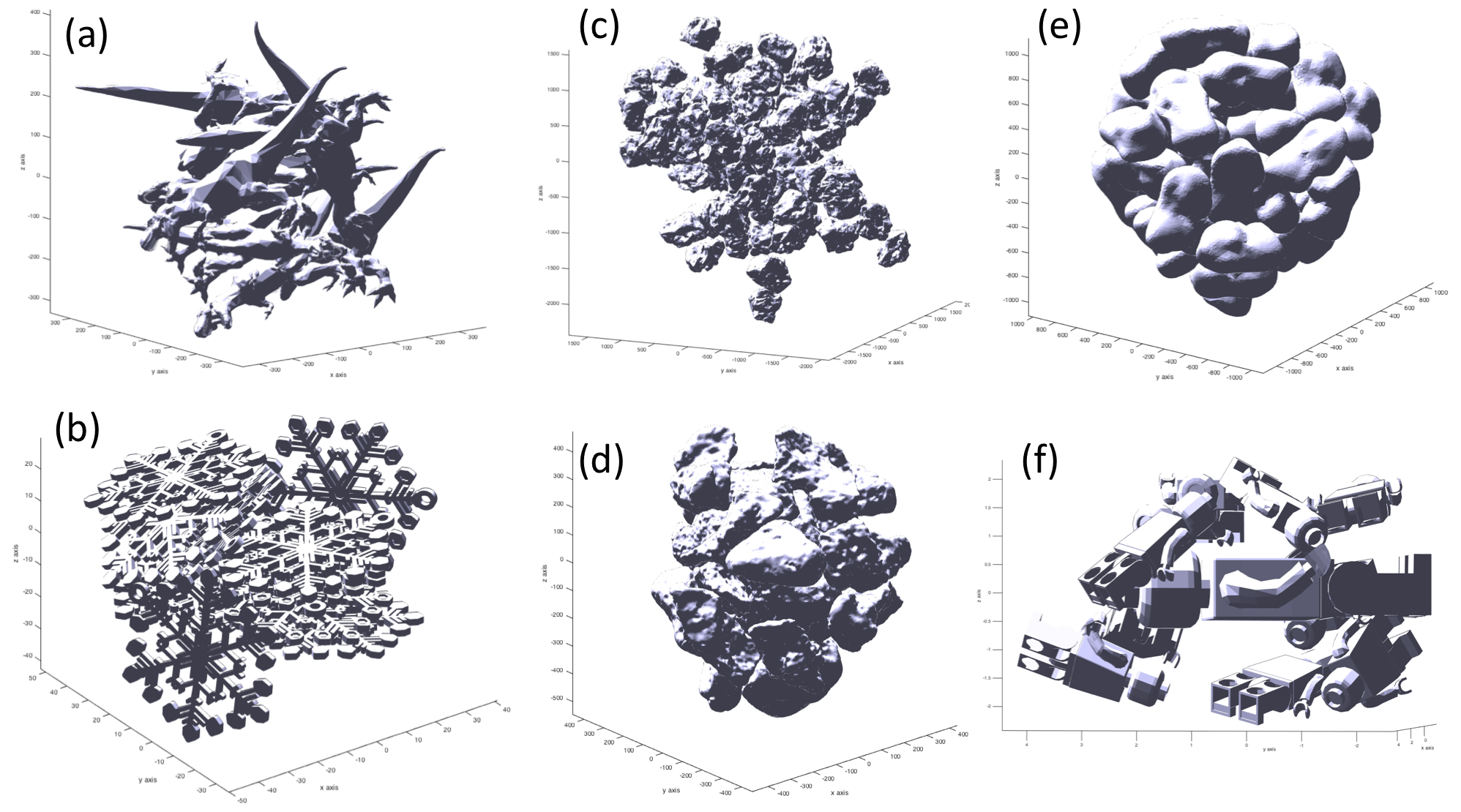
Figure A1 Virtual aggregates made of different initial STL files: (a) aggregate made from an STL file of a T-rex, (b) aggregate made from an STL file of snowflakes, (c) aggregate made of real volcanic particles scanned with a 3D laser scanning machine (loose packing), (d) the same shapes and objects in (c) but with tighter packing, (e) aggregate made using as an STL file the asteroid Castalia, and (f) aggregate made of toy characters.