the Creative Commons Attribution 4.0 License.
the Creative Commons Attribution 4.0 License.
 | 09 Jul 2021
Efficient Bayesian inference for large chaotic dynamical systems
Sebastian Springer
Heikki Haario
Jouni Susiluoto
Aleksandr Bibov
Andrew Davis
Youssef Marzouk
Estimating parameters of chaotic geophysical models is challenging due to their inherent unpredictability. These models cannot be calibrated with standard least squares or filtering methods if observations are temporally sparse. Obvious remedies, such as averaging over temporal and spatial data to characterize the mean behavior, do not capture the subtleties of the underlying dynamics. We perform Bayesian inference of parameters in high-dimensional and computationally demanding chaotic dynamical systems by combining two approaches: (i) measuring model–data mismatch by comparing chaotic attractors and (ii) mitigating the computational cost of inference by using surrogate models. Specifically, we construct a likelihood function suited to chaotic models by evaluating a distribution over distances between points in the phase space; this distribution defines a summary statistic that depends on the geometry of the attractor, rather than on pointwise matching of trajectories. This statistic is computationally expensive to simulate, compounding the usual challenges of Bayesian computation with physical models. Thus, we develop an inexpensive surrogate for the log likelihood with the local approximation Markov chain Monte Carlo method, which in our simulations reduces the time required for accurate inference by orders of magnitude. We investigate the behavior of the resulting algorithm with two smaller-scale problems and then use a quasi-geostrophic model to demonstrate its large-scale application.
- Article
(8517 KB) - Full-text XML
-
Supplement
(1344 KB) - BibTeX
- EndNote


Time evolution of many geophysical dynamical systems is chaotic. Chaoticity means that state of a system sufficiently far in the future cannot be predicted even if we know the dynamics and the initial conditions very precisely. Commonly used examples of chaotic systems include climate, weather, and the solar system.
A system being chaotic does not mean that it is random: the dynamics of models of chaotic systems are still determined by parameters, which may be either deterministic or random (Gelman et al., 2013). For example, Monte Carlo methods may be used to simulate future climate variability, but the distribution of possible climates will depend on the parameters of the climate model, and using the wrong model parameter distribution will result in potentially biased results with inaccurate uncertainties. For this reason, parameter estimation in chaotic models is an important problem for a range of geophysical applications. This paper focuses on Bayesian approaches to parameter inference in settings where (a) model dynamics are chaotic, and (b) sequential observations of the system are obtained so rarely that the model behavior has become unpredictable.
Parameters of a dynamical system model are most commonly inferred by minimizing a cost function that captures model–observation mismatch (Tarantola, 2005). In the Bayesian setting (Gelman et al., 2013), modeling this mismatch probabilistically yields a likelihood function, which enables maximum likelihood estimation or fully Bayesian inference. In fully Bayesian inference, the problem is further regularized by prescribing a prior distribution on the model state. In practice, Bayesian inference is often realized via Markov chain Monte Carlo (MCMC) methods (Gamerman, 1997; Robert and Casella, 2004).
This straightforward strategy – for instance, using the squared Euclidean distance between model outputs and data to construct a Gaussian likelihood – is, however, inadequate for chaotic models, where small changes in parameters, or even in the tolerances used for numerical solvers, can lead to arbitrarily large differences in model outputs (Rougier, 2013). Furthermore, modeling dynamical systems is often computationally very demanding, which makes sample generation time consuming. Since successful application of MCMC generally requires large numbers of model evaluations, performing Bayesian inference with MCMC is often not possible.
The present works combines two recent methods to tackle these problems due to model chaoticity and computational cost. Chaoticity is tamed by using correlation integral likelihood (CIL) (Haario et al., 2015), which is able to constrain the parameters of chaotic dynamical systems. We couple CIL with local approximation MCMC (LA-MCMC) (Conrad et al., 2016), which is a surrogate modeling technique that makes asymptotically exact posterior characterization feasible for computationally expensive models. We show how combining these methods enables a Bayesian approach to infer the parameters of chaotic high-dimensional models and quantify their uncertainties in situations previously discussed as intractable (Rougier, 2013). Moreover, we introduce several computational improvements to further enhance the applicability of the approach.
The CIL method is based on the concept of fractal dimension from mathematical physics, which broadly speaking characterizes the space-filling properties of the trajectory of a dynamical system. Earlier work (e.g., Cencini et al., 2010) describes a number of different approaches for estimating the fractal dimension. Our previous work extends this concept: instead of computing the fractal dimension of a single trajectory, a similar computation measures the distance between different model trajectories (Haario et al., 2015), based on which a specific summary statistic, called feature vector, is computed. The modification provides a normally distributed statistic of the data, which is sensitive to changes in the underlying attractor from which the data were sampled. Statistics that are sensitive to changes in the attractor yield likelihood functions that can better constrain the model parameters and therefore also result in more meaningful parameter posterior distributions.
The LA-MCMC method (Conrad et al., 2016, 2018) approximates the computationally expensive log-likelihood function using local polynomial regression. In this method, the MCMC sampler directly uses the approximation of the log likelihood to construct proposals and evaluate the Metropolis acceptance probability. Infrequently but regularly adding “full” likelihood evaluations to the point set used to construct the local polynomial regression continually improves the approximation, however. Expensive full likelihood evaluations are thus used only to construct the approximation or “surrogate” model. Conrad et al. (2016) show that, given an appropriate mechanism for triggering likelihood evaluations, the resulting Markov chain converges to the true posterior distribution while reducing the number of expensive likelihood evaluations (and hence forward model simulations) by orders of magnitude. Davis et al. (2020) show that LA-MCMC converges with approximately the expected error decay rate after a finite number of steps T, and Davis (2018) introduces a numerical parameter that ensures convergence even if only noisy estimates of the target density are available. This modification is useful for the chaotic systems studied here.
The rest of this paper is organized as follows. Section 2 reviews some additional background literature and related work and Sect. 3 describes the methodologies used in this work, including the CIL, the stochastic LA-MCMC algorithm, and the merging of these two approaches. Section 4 is dedicated to numerical experiments, where the CIL/LA-MCMC approach is applied to several, progressively more demanding examples. These examples are followed by a concluding discussion in Sect. 5.
Traditional parameter estimation methods, which directly utilize the model–observation mismatch, constrain the modeling to limited time intervals when the model is chaotic. This avoids the eventual divergence (chaotic behavior) of orbits that are initially close to each other. A classical example is variational data assimilation for weather prediction, where the initial states of the model are estimated using observational data and algorithms such as 4D-Var, after which a short-time forecast can be simulated (Asch et al., 2016).
Sequential data assimilation methods, such as the Kalman filter (KF) (Law et al., 2015), allow parameter estimation by recursively updating both the model state and the model parameters by conditioning them on observational data obtained over sufficiently short timescales. With methods such as state augmentation, model parameters can be updated as part of the filtering problem (Liu and West, 2001). Alternatively, the state values can be integrated out to obtain the marginal likelihood over the model parameters (Durbin and Koopman, 2012). Hakkarainen et al. (2012) use this filter likelihood approach to estimate parameters of chaotic systems. For models with strongly non-linear dynamics, ensemble filtering methods provide a useful alternative to the extended Kalman filter or variational methods; see Houtekamer and Zhang (2016) for a recent review of various ensemble variants.
Filtering-based approaches generally introduce additional tuning parameters, such as the length of the assimilation time window, the model error covariance matrix, and covariance inflation parameters. These choices have an impact on model parameter estimation and may introduce bias. Indeed, as discussed in Hakkarainen et al. (2013), changing the filtering method requires updating the parameters of the dynamical model. Alternatives to KF-based parameter estimation methods that do not require ensemble filtering include operational ensemble prediction systems (EPSs); for example, ensemble parameter calibration methods by Jarvinen et al. (2011) and Laine et al. (2011) have been applied to the Integrated Forecast System (IFS) weather models (Ollinaho et al., 2012, 2013, 2014) at the European Centre for Medium-Range Weather Forecasts (ECMWF). However, these approaches are heuristic and again limited to relatively short predictive windows.
Climate model parameters have in previous studies (e.g., Roeckner et al., 2003; ECMWF, 2013; Stevens et al., 2013) been calibrated by matching summary statistics of quantities of interest, such as top-of-atmosphere radiation, with the corresponding summary statistics from reanalysis data or output from competing models. The vast majority of these approaches produce only point estimates. A fully Bayesian parameter inversion was performed by Järvinen et al. (2010), who inferred closure parameters of a large-scale computationally intensive climate model, ECHAM5, using MCMC and several different summary statistics.
Computational limitations make applying algorithms such as MCMC challenging for weather and climate models. Generating even very short MCMC chains may require methods such as parallel sampling and early rejection for tractability (Solonen et al., 2012). Moreover, even if these computational challenges can be overcome, finding statistics that actually constrain the parameters is difficult, and inference results can be thus be inconclusive. The failure of the summary statistic approach in Järvinen et al. (2010) can be explained intuitively: the chosen statistics average out too much information and therefore fail to characterize the geometry of the underlying chaotic attractor in a meaningful way.
Several Monte Carlo methods have been presented to tackle expensive or intractable likelihoods; see, e.g., Luego et al. (2020) for a recent comprehensive literature review. Two notable such methods are approximate Bayesian computation (ABC) (Beaumont et al., 2002) and pseudo-marginal sampling (Andrieu and Roberts, 2009). The approach that is most closely related to the one presented in this paper is Bayesian inference using synthetic likelihoods, which was proposed as an alternative to ABC (Wood, 2010; Price et al., 2018). Recent work by Morzfeld et al. (2018) describes another feature vector approach for data assimilation. For more details and comparisons among these approaches, see the discussion below in Sect. 3.1.
In this work, we employ a different summary statistic, where the observations are considered as samples from the underlying attractor. Due to the nature of the summary statistic used in CIL, the observation time stamps are not explicitly used. This allows arbitrarily sparse observation time series, and consecutive observations may be farther than any window where the system remains predictable. To the best of our knowledge, parameter estimation in this setting has not been discussed in the literature. Another difference with the synthetic likelihood approach is that it involves regenerating data for computing the likelihood at every new model parameter value, which would be computationally unfeasible in our setting.
3.1 Correlation integral likelihood
We first construct a likelihood function that models the observations by comparing certain summary statistics of the observations to the corresponding statistics of a trajectory simulated from the chaotic model. As a source of statistics, we will choose the correlation integral, which depends on the fractal dimension of the chaotic attractor. Unlike other statistics – such as the ergodic averages of a trajectory – the correlation integral is able to constrain the parameters of a chaotic model (Haario et al., 2015).
Let us denote by
a dynamical system with state u(t)∈ℝn, initial state u0∈ℝn, and parameters θ∈ℝq. The time-discretized system, with time steps denoting selected observation points, can be written as
Either the full state ui∈ℝn or a subset of the state components are observed. We will use to denote a collection of these observables at successive times.
Using the model–observation mismatch at a collection of times ti to constrain the value of the parameters θ is not suitable when the system (1) has chaotic dynamics, since the state vector values si are unpredictable after a finite time interval. Though long-time trajectories s(t) of chaotic systems are not predictable in the time domain, they do, however, represent samples from an underlying attractor in the phase space. The states are generated deterministically, but the model's chaotic nature allows us to interpret the states as samples from a particular θ-dependent distribution. Yet obvious choices for summary statistics T that depend on the observed states S, such as ergodic averages, ignore important aspects of the dynamics and are thus unable to constrain the model parameters. For example, the statistic is easy to compute and is normally distributed in the limit τ→∞ (under appropriate conditions), but this ergodic mean says very little about the shape of the chaotic attractor.
Instead, we need a summary statistic that retains information relevant for parameter estimation but still defines a computationally tractable likelihood. To this end, Haario et al. (2015) devised the CIL, which retains enough information about the attractor to constrain the model parameters. We first review the CIL and then discuss how to make evaluation of the likelihood tractable.
We will use the CIL to evaluate the “difference” between two chaotic attractors. For this purpose, we will first describe how to statistically characterize the geometry of a given attractor, given suitable observations S. In particular, constructing the CIL likelihood will require three steps: (i) computing distances between observables sampled from a given attractor; (ii) evaluating the empirical cumulative distribution function (ECDF) of these distances and deriving certain summary statistics T from the ECDF; and (iii) estimating the mean and covariance of T by repeating steps (i) and (ii).
Intuitively, the CIL thus interprets observations of a chaotic trajectory as samples from a fixed distribution over phase space. It allows the time between observations to be arbitrarily large – importantly, much longer than the system's non-chaotic prediction window.
Now we describe the CIL construction in detail. Suppose that we have collected a data set S comprising observations of the dynamical system of interest. Let S be split into nepo different subsets called epochs. The epochs can, in principle, be any subsets of length N from the reference data set S. In this paper, however, we restrict the epochs to be time-consecutive intervals of N evenly spaced observations. Let and , with and k≠l, be two such disjoint epochs. The individual observable vectors and comprising each epoch come from time intervals and , respectively. In other words, superscripts refer to different epochs and subscripts refer to the time points within those epochs. Haario et al. (2015) then define the modified correlation integral sum by counting all pairs of observations that are less than a distance R>0 from each other:
where 1 denotes the indicator function and is the Euclidean norm on ℝd. In the physics literature, evaluating Eq. (3) in the limit R→0, with k=l and i≠j, numerically approximates the fractal dimension of the attractor that produced sk=sl (Grassberger and Procaccia, 1983a, b). Here, we instead use Eq. (3) to characterize the distribution of distances between sk and sl at all relevant scales. We assume that the state space is bounded; therefore, an R0 covering all pairwise distances in Eq. (3) exists. For a prescribed set of radii , with b>1 and , Eq. (3) defines a discretization of the ECDF of the distances , with discretization boundaries given by the numbers Rm.
Now we define as components of a statistic . This statistic is also called the feature vector. According to Borovkova et al. (2001) and Neumeyer (2004), the vectors yk,l are normally distributed, and the estimates of the mean and covariance converge at the rate to their limit points. This is a generalization of the classical result of Donsker (1951), which applies to Independent and identically distributed samples from a scalar-valued distribution. We characterize this normal distribution by subsampling the full data set S. Specifically, we approximate the mean μ and covariance Σ of T by the sample mean and sample covariance of the set , evaluated for all pairs of epochs (sk,sl) using fixed values of R0, b, M, and N.
The Gaussian distribution of T effectively characterizes the geometry of the attractor represented in the data set S. Now we wish to use this distribution to infer the parameters θ. Given a candidate parameter value , we use the model to generate states for the length of a single epoch. We then evaluate the statistics as in Eq. (3), by computing the distances between elements of and the states of an epoch sk selected from the data S. Combining these statistics into a feature vector , we can write a noisy estimate of the log-likelihood function:
Comparing with other epochs drawn from the data set S, however, will produce different realizations of the feature vector. We thus average the resulting log likelihoods over all epochs:
This averaging, which involves evaluating Eq. (4) nepo times, involves only new distance computations and is thus relatively cheap relative to time integration of the dynamical model.
Because the feature vectors are random for any finite N, and because the number of epochs nepo is also finite, the log likelihood in Eq. (5) is necessarily random. It is then useful to view Eq. (5) as estimate of an underlying true log likelihood. We are therefore in a setting where cannot evaluate the unnormalized posterior density exactly; we only have access to a noisy approximation of it. Previous work (Springer et al., 2019) has demonstrated that derivative-free optimizers such as the differential evolution (DE) algorithm can successfully identify the posterior mode in this setting, yielding a point estimate of θ. In the fully Bayesian setting, one could characterize the posterior p(θ|S) using pseudo-marginal MCMC methods (Andrieu and Roberts, 2009) but at significant computational expense. Below, we will use a surrogate model constructed adaptively during MCMC sampling to reduce this computational burden.
Note that the CIL approach described above already reduces the computational cost of inference by only requiring simulation of the (potentially expensive) chaotic model for a single epoch. We compare each epoch of the data to the same single-epoch model output. Each of these comparisons results in an estimate of the log likelihood, which we then average over data epochs. A larger data set S can reduce the variance of this average, but does not require additional simulations of the dynamical model. Also, we do not require any knowledge about the initial conditions of the model; we omit an initial time interval before extracting to ensure that the observed trajectory is on the chaotic attractor.
Moreover, the initial values are randomized for all simulations and sampling is started only after the model has integrated beyond the initial, predictable, time window. The independence of the sampled parameter posteriors from the initial values was verified both here and in earlier works by repeated experiments.
Our approach is broadly similar to the synthetic likelihood method (e.g., Wood, 2010; Price et al., 2018) but differs in two key respects: (i) we use a novel summary statistic that is able to characterize chaotic attractors, and (ii) we only need to evaluate the forward model for a single epoch. Comparatively, synthetic likelihoods typically use summary statistics such as auto-covariances at a given lag or regression coefficients. These methods also require long-time integration of the forward model for each candidate parameter value θ, rather than integration for only one epoch. Morzfeld et al. (2018) also discuss several ways of using feature vectors for inference in geophysics. A distinction of the present work is that we use an ECDF-based summary statistic that is provably Gaussian, and we perform extensive Bayesian analysis of the parameter posteriors via novel MCMC methods. These methods are described next.
3.2 Local approximation MCMC
Even with the developments described above, estimating the CIL at each candidate parameter value is computationally intensive. We thus use local approximation MCMC (LA-MCMC) (Conrad et al., 2016, 2018; Davis et al., 2020) – a surrogate modeling method that replaces many of these CIL evaluations with an inexpensive approximation. Replacing expensive density evaluations with a surrogate was first introduced by Sacks et al. (1989) and Kennedy and O'Hagan (2001). LA-MCMC extends these ideas by continually refining the surrogate during sampling, which guarantees convergence.
First introduced in Conrad et al. (2016), LA-MCMC builds local surrogate models for the log likelihood while simultaneously sampling the posterior. The surrogate is incrementally and infinitely refined during sampling and thus tailored to the problem – i.e., made more accurate in regions of high posterior probability. Specifically, the surrogate model is a local polynomial computed by fitting nearby evaluations of the “true” log likelihood. We emphasize that the approximation itself is not locally supported. At each point , we locally construct a polynomial approximation, which globally defines a piecewise polynomial surrogate model. This is an important distinction because the piecewise polynomial approximation is not necessarily a probability density function. In fact, the surrogate function may not even be integrable. Despite this challenge, Davis et al. (2020) devise a refinement strategy that ensures convergence and bounds the error after a finite number of samples. In particular, Davis et al. (2020) shows that the error in the approximate Markov chain computed with the local surrogate model decays at approximately the expected rate, where T is the number of MCMC steps. Davis (2018) demonstrated that noisy estimates of the likelihood are sufficient to construct the surrogate model and still retain asymptotic convergence. Empirical studies (Conrad et al., 2016, 2018; Davis et al., 2020) on problems of moderate parameter dimension showed that the number of expensive likelihood evaluations per MCMC step can be reduced by orders of magnitude, with no discernable loss of accuracy in posterior expectations.
Here, we briefly summarize one step of the LA-MCMC construction and refer to Davis et al. (2020) for details. Each LA-MCMC step consists of four stages: (i) possibly refine the local polynomial approximation of the log likelihood, (ii) propose a new candidate MCMC state, (iii) compute the acceptance probability, and (iv) accept or reject the proposed state. The major distinction between this algorithm and standard Metropolis–Hastings MCMC is that the acceptance probability in stage (iii) is computed only using the approximation or surrogate model of the log likelihood, at both the current and proposed states. This introduces an error, relative to computation of the acceptance probability with exact likelihood evaluations, but stage (i) of the algorithm is designed to control and incrementally reduce this error at the appropriate rate.
“Refinement” in stage (i) consists of adding a computationally intensive log-likelihood evaluation at some parameter value θi, denoted by ℒ(θi), to the evaluated set . These K pairs are used to construct the local approximation via a kernel-weighted local polynomial regression (Kohler, 2002). The values are called “support points” in this paper. Details on the regression formulation are in Davis et al. (2020); Conrad et al. (2016). As the support points cover the regions of high posterior probability more densely, the accuracy of the local polynomial surrogate will increase. This error is well understood (Kohler, 2002; Conn et al., 2009) and, crucially, takes advantage of smoothness in the underlying true log-likelihood function. This smoothness ultimately allows the cardinality of the evaluated set to be much smaller than the number of MCMC steps.
Intuitively, if the surrogate converges to the true log likelihood, then the samples generated with LA-MCMC will (asymptotically) be drawn from the true posterior distribution. After any finite number of steps, however, the surrogate error introduces a bias into the sampling algorithm. The refinement strategy must therefore ensure that this bias is not the dominant source of error. At the same time, refinements must occur infrequently to ensure that LA-MCMC is computationally cheaper than using the true log likelihood. Davis et al. (2020) analyzes the trade-off between surrogate-induced bias and MCMC variance and proposes a rate-optimal refinement strategy. We use a similar algorithm, only adding an isotropic ℓ2 penalty on the polynomial coefficients. More specifically, we rescale the variables so the max/min values are ±1 – often called coded units – then regularize the regression by a penalty parameter (in our cases, the value α=1 was found sufficient). This penalty term modifies the ordinary least squares problem into local ridge regression, which improves performance with noisy likelihoods.
Our examples use an adaptive proposal density Haario et al. (2006). This choice deviates slightly from the theory in Davis et al. (2020), which assumes a constant-in-time proposal density. However, this does not necessarily imply that adaptive or gradient-based methods will not converge. In particular, Conrad et al. (2016) show asymptotic convergence using an adaptive proposal density and Conrad et al. (2018) strengthen this result by showing that the Metropolis-adjusted Langevin algorithm, which is a gradient based MCMC method, is asymptotically exact when using a continually refined local polynomial approximation. These results require some additional assumptions about the target density's tail behavior and the stronger rate optimal result from Davis et al. (2020) has not been shown for such algorithms. However, in practice, we see that adaptive methods still work well in our applications. Exploring the theoretical implications of this is interesting and merits further discussion but is beyond the scope of this paper.
The parameters of the algorithm are fixed as given in Davis et al. (2020), for all the examples discussed here: (i) initial error threshold γ0=1; (ii) error threshold decay rate γ1=1; (iii) maximum poisedness constant ; (iv) tail-correction parameter η=0 (no tail correction); (v) local polynomial degree p=2. The number of nearest neighbors k used to construct each local polynomial surrogate is chosen to be where , q is the dimension of the parameters θ∈ℝq, and D is the number of coefficients in the local polynomial approximation of total degree p=2, i.e., . If we had k=D, the approximation would be an interpolant. Instead, we oversample by a factor , as suggested in Conrad et al. (2016), and allow k to grow slowly with the size K of the evaluated set as in Davis (2018). All these details together with example runs can be found in the MATLAB implementation available in the Supplement.
This section contains numerical experiments to illustrate the methods introduced in the previous sections. As a large-scale example, we characterize the posterior distribution of parameters in the two-layer quasi-geostrophic (QG) model. The computations needed to characterize the posterior distribution with standard MCMC methods in this example would be prohibitive without massive computational resources and are therefore omitted. In contrast, we will show that the LA-MCMC method is able to simulate from the parameter posterior distribution.
Before presenting this example, we first demonstrate that the posteriors produced by LA-MCMC agree with those obtained via exact MCMC sampling methods in cases where the latter are computationally tractable using two examples: the classical Lorenz 63 system and the higher-dimensional Kuramoto–Sivashinsky (KS) model. In both examples, we quantify the computational savings due to LA-MCMC, and in the second we introduce additional ways to speed up computation using parallel (GPU) integration.
Let Δt denote the time difference between consecutive observations; one epoch thus contains the times in the interval . The number of data points in one epoch N varies between 1000 and 2000, depending on the example. The training set S consists of a collection of nepo such intervals. In all the examples, we choose Δt to be relatively large, beyond the predictable window. This is more for demonstration purposes than a necessity; the background theory from U statistics allows the subsequent state vectors to be weakly dependent. Numerically, a set of observations that is chosen too densely results in the χ2 test failing, and for this reason we recommended to always check for normality before starting the parameter estimation.
For numerical tests, one can either use one long time series or integrate a shorter time interval several times using different initial values to create the training set for the likelihood. For these experiments, the latter method was used with nepo=64, yielding different pairs (sk,sl), each of which resulted in an ECDF constructed from N2 pairwise distances. According to tests performed while calibrating the algorithm, these values of N and nepo are sufficient to obtain robust posterior estimates. With less data, the parameter posteriors will be less precise.
The range of the bin radii is selected by examining the distances within the training set, keeping in mind that a positive variance is needed for every bin to avoid a singular covariance matrix. So the largest radius R0 can be obtained from
over the disjoint subsets of the samples sk and sl of length N. The smallest radius is selected by requiring that for all the possible pairs (sk,sl), it holds that , where is the ball of radius RM centered at . That is,
The base value b is obtained by , and using this value we fix all the other radii Rm.
As always with histograms, the number of bins M must be selected first. Too small an M loses information, while too large values yield noisy histograms, and this noisiness can be seen also in the ECDFs. However, numerical experiments show that the final results – the parameter posteriors – are not too sensitive to the specific value of M. For instance, for the Lorenz 63 case below, the range of M was varied between 5 and 40, and only a minor decrease of the size of the parameter posteriors was noticed for increasing M. Any slight increase of accuracy comes with a computational cost: higher values of M increase the stochasticity of the likelihood evaluations, which leads to smaller acceptance rates in the MCMC sampling, e.g., from 0.36 to 0.17 to 0.03 for , respectively, when using the standard adaptive Metropolis sampler. In the examples presented in this section, the length M of the feature vector is fixed to 14 for the Lorenz 63 model and 32 for the higher-dimensional KS and QG models.
To balance the possibly different magnitudes of the components of the state vector, each component is scaled and shifted to the range before computing the distances. While this scaling could also be performed in other ways, this method worked well in practice for the models considered. The normality of the ensemble of feature vectors is ascertained by comparing the histograms of the quadratic forms in Eq. (4) visually to the appropriate χ2 distribution.
In all the three experiments, we create MCMC chains of length 105. However, due to the use of the LA-MCMC approach, the number of full forward model evaluations is much lower, around 1000 or less; we will report these values more specifically below.
The Lorenz 63 model was integrated with a standard Runge–Kutta solver. The numerical solution of the KS-model is based on our in-house fast Fourier transform (FFT)-based solver, which runs on the GPU side and is built around Nvidia compute unified device architecture (CUDA) toolchain and cuFFT library (which is a part of the CUDA ecosystem). The quasi-geostrophic model employs semi-Lagrangian solver and runs entirely on CPU, but the code has been significantly optimized with performance-critical parts, such as advection operator, compiled using an Intel single program compiler (ISPC) with support of Advanced Vector Extensions 2 (AVX2) vectorization.
4.1 Lorenz 63
We use the classical three-dimensional Lorenz 63 system (Lorenz, 1963) as a simple first example to demonstrate how LA-MCMC can be successfully paired with the CIL and the adaptive Metropolis (AM) algorithm (Haario et al., 2001, 2006) to obtain the posterior distribution for chaotic systems at a greatly reduced computational cost, compared to AM without the local approximation. The time evolution of the state vector is given by
This system of equations is often said to describe an extreme simplification of a weather model.
The reference data were generated with parameter values σ=10, ρ=28, and by performing nepo=64 distinct model simulations, with observations made at 2000 evenly distributed times between [10,20 000]. These observations were perturbed with 5 % multiplicative Gaussian noise. The length of the predictable time window is roughly 7, which is less than the time between consecutive observations. The parameters of the CIL method were obtained as described at the start of Sect. 4, with values M=14, R0=2.85, and b=1.51.
The set of vectors is shown in Fig. 1 in the log–log scale. The figure shows how the variability of these vectors is quite small. Figure 1 validates the normality assumption for feature vectors.
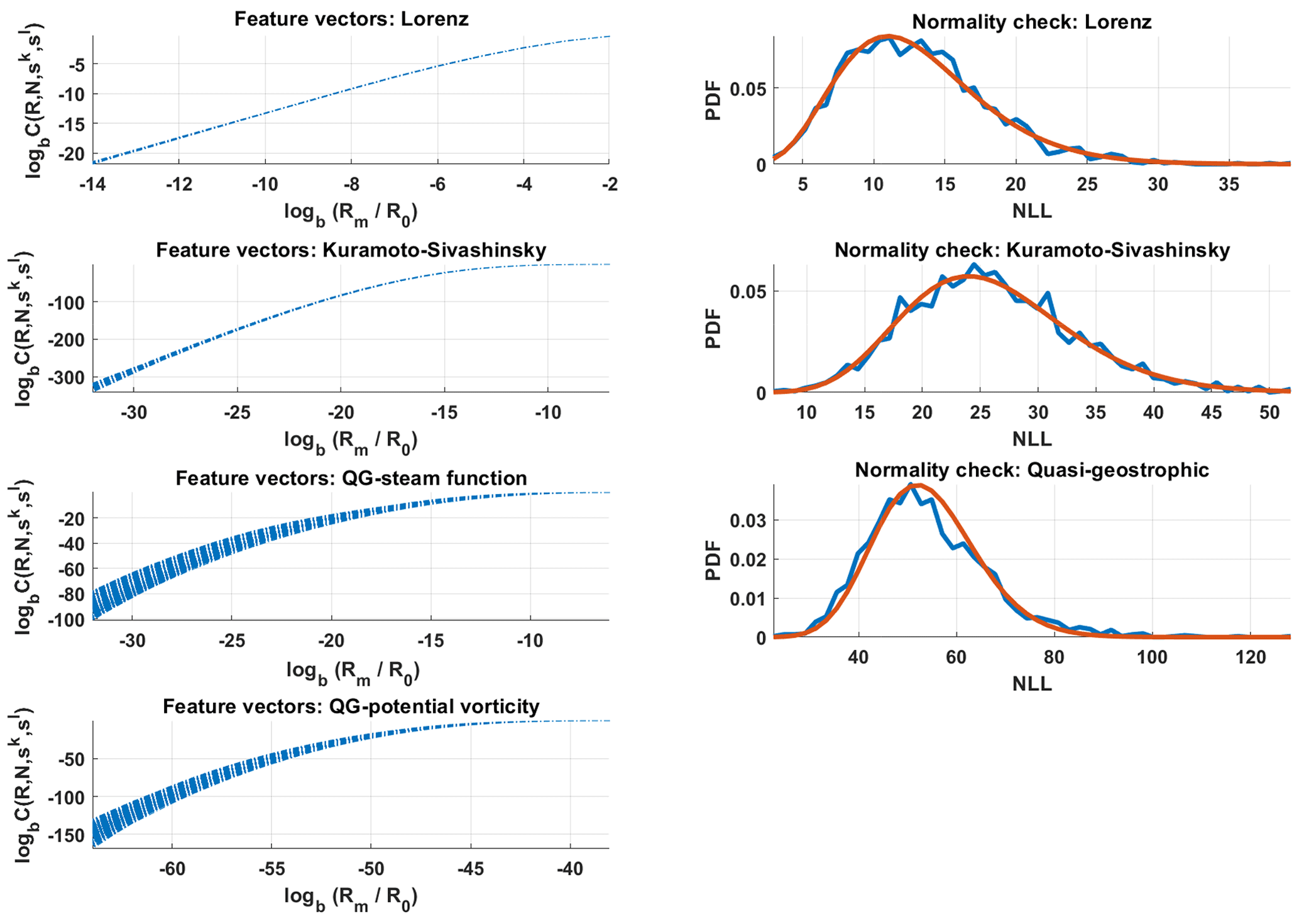
Figure 1Left: for all combinations of k and l, the feature vectors for Lorenz 63 and Kuramoto–Sivashinsky, along with concatenated feature vectors for the quasi-geostrophic system are shown. Right: normality check; the χ2 density function versus the histograms of the respective negative log-likelihood (NLL) values; see Eq. (4).
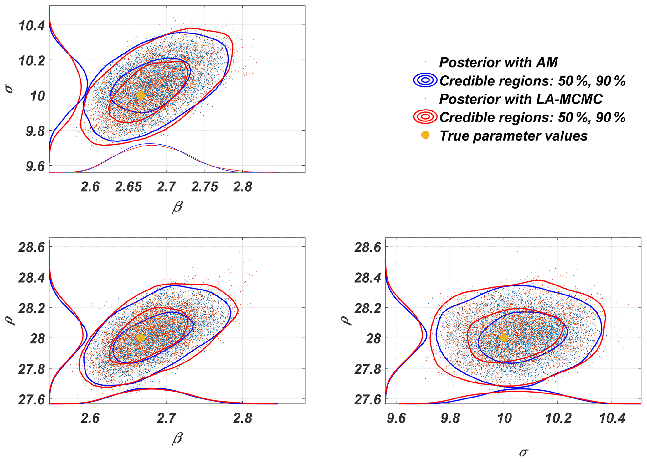
Figure 2Two-dimensional posterior marginal distributions of the parameters of the Lorenz 63 model obtained with LA-MCMC and AM.
Pairwise two-dimensional marginals of the parameter posterior are shown in Fig. 2, both from sampling the posterior with full forward model simulations (AM) and with using the surrogate sampling approach for generating the chain. These two posteriors are almost perfectly superimposed. Indeed, the difference is at the same level as that between repetitions of the standard AM sampling alone.
To get an idea of the computational savings achieved with LA-MCMC, the computation of the MCMC chains of length 105 was repeated 10 times. The cumulative number of full likelihood evaluations is presented in Fig. 3. At the end of the chains, the number of full likelihood evaluations varied between 955 and 1016. Thus, by using LA-MCMC in this setting, remarkable computational savings of up to 2 orders of magnitude are achieved.
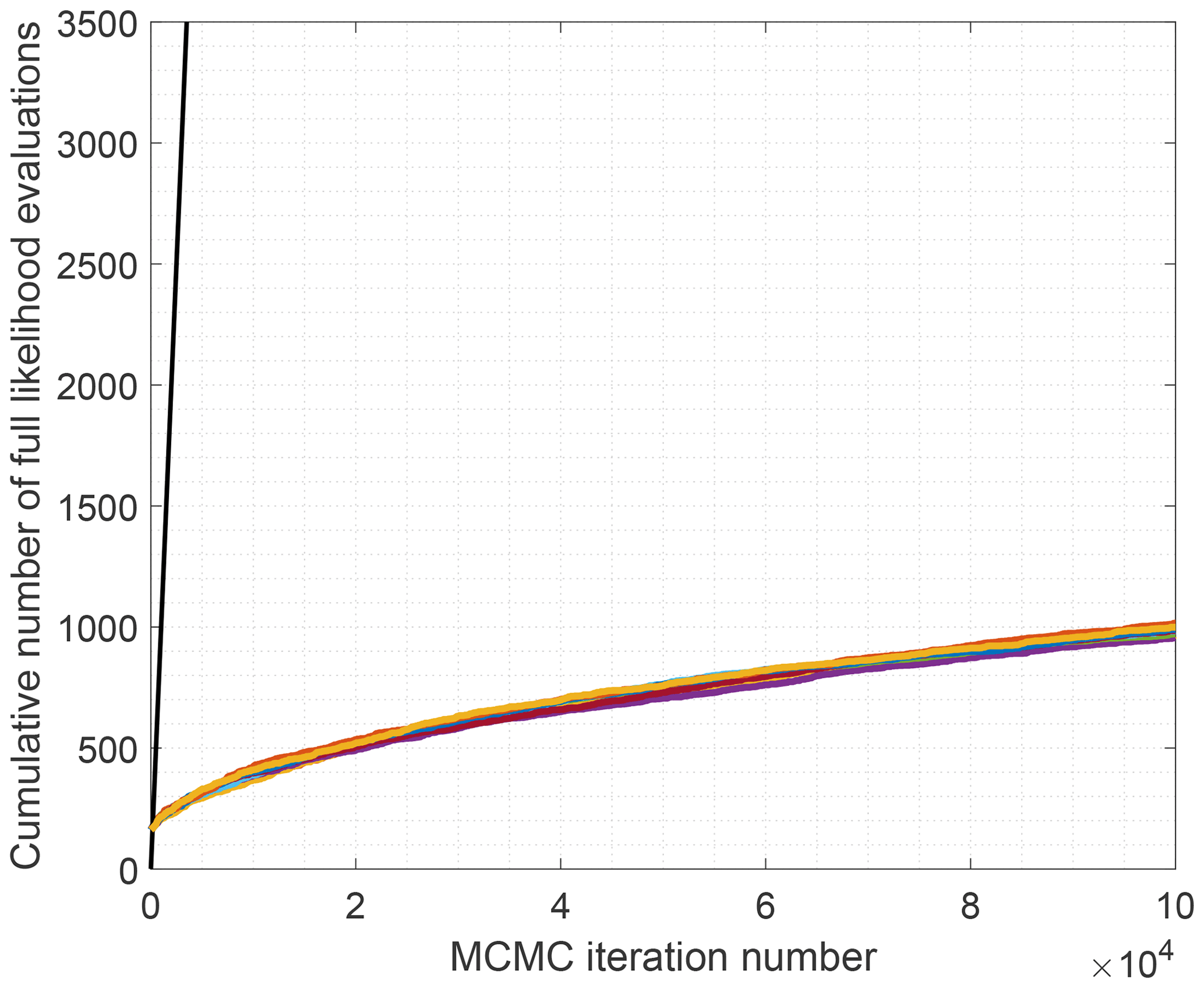
Figure 3Comparison of the cumulative number of full likelihood evaluations while using AM (black line) and LA-MCMC (colored lines). Every colored line correspond to a different chain obtained with LA-MCMC by using the same likelihood.
4.2 The Kuramoto–Sivashinsky model
The second example is the 256-dimensional Kuramoto–Sivashinsky (KS) partial differential equation (PDE) system. The purpose of this example is to introduce ways to improve the computational efficiency by a piecewise parallel integration over the time interval of given data. Also, we demonstrate how decreasing the number of observed components impacts the accuracy of parameter estimation. Even though the posterior evaluation proves to be relatively expensive, direct verification of the results with those obtained by using standard adaptive MCMC is still possible. The Kuramoto–Sivashinsky model is given by the fourth-order PDE:
where is a real function of x∈ℝ and . In addition, it is assumed that s is spatially periodical with period of L, i.e., . This experiment uses the parametrization from (Yiorgos Smyrlis, 1996) that maps the spatial domain to by setting and . With L=100, the true value of parameter γ is , and the true value of η becomes . These two parameters are the ones that are then estimated with the LA-MCMC method. This system was derived by Kuramoto and Yamada (1976) and Kuramoto (1978) as a model for phase turbulence in reaction–diffusion systems. Sivashinsky (1977) used the same system for describing instabilities of laminar flames.
Assume that the solution for this problem can be represented by a truncation of the Fourier series
Using this form reduces Eq. (9) to a system of ordinary differential equations for the unknown coefficients Aj(t) and Bj(t),
where the terms F1(⋅) and F2(⋅) are polynomials of the vectors A and B. For details, see Huttunen et al. (2018). The solution can be effectively computed on graphics processors in parallel, and if computational resources allow, several instances of Eq. (9) can be solved in parallel. Even on fast consumer-level laptops, several thousand simulations can be performed in parallel when the discretization of the x dimension contains around 500 points.
A total of 64 epochs of the 256-dimensional KS model are integrated over the time interval [0,150 000], and as in the case of the Lorenz 63 model, the initial predictable time window is discarded and 1024 equidistant measurements from [500,150 000] are selected, with Δt≈146. The parameters used for the CIL method were R0=1801.7, M=32, and b=1.025.
The time needed to integrate the model up to t=150 000 is approximately 103 s with the Nvidia 1070 GPU, implying that generating an MCMC chain with 100 000 samples with standard MCMC algorithms would take almost 4 months. The use of LA-MCMC alone again shortens the time needed by a factor of 100 to around 28 h. However, the calculations can yet be considerably enhanced by parallel computing. In practice, this translates the problem of generating a candidate trajectory of length 150 000 into generating observations from several shorter time intervals. In our example, an efficient division is to perform 128 parallel calculations each of length 4500, with randomized initial values close to the values selected from the training set. Discarding the predictable interval [0,500] and taking eight observations at intervals of 500 yields the same number (1024) of observations as in the initial setting. While the total integration time increases, this reduces the wall-clock time needed for computation of a single candidate simulation from 103 to 2.5 s. The full MCMC chain can be then be generated in 70 h without the surrogate model and in 42 min using LA-MCMC.
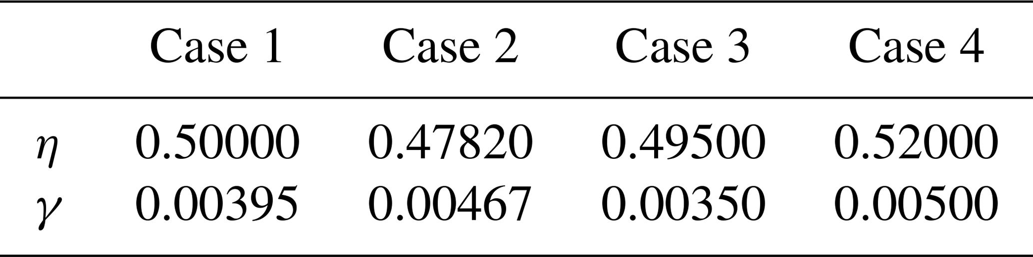
Table 1Parameter values of the four parameter vectors used in the forward KS model simulation examples in Fig. 5. The parameter vectors in the first column labeled 1 are the true parameters, and the second one resides inside the posterior. The last two are outside the posterior. These parameters correspond to points shown in the posterior distribution shown in Fig. 4.
Parameter posterior distributions from the KS system, produced with MCMC both with and without the local approximation surrogate, are shown in Fig. 4. Repeating the calculations several times yielded no meaningful differences in the results. In this experiment, the number of forward model evaluations LA-MCMC needed for generating a chain of length 100 000 was in the range [1131,1221].
Model trajectories from simulations with four different parameter vectors are shown in Fig. 5. These parameter values were (1) the “true” value which was used to generate training data, (2) another parameter from inside the posterior distribution, and (3–4) two other parameters from outside the posterior distribution. These parameters are also shown in Fig. 4. Visually inspecting the outputs, cases 1–3 look similar, while results using parameter vector 4, furthest away from the posterior, are markedly different. Even though the third parameter vector is outside the posterior, the resulting trajectory is not easily distinguishable from cases 1 and 2, indicating that the CIL method differentiates between the trajectories more efficiently.
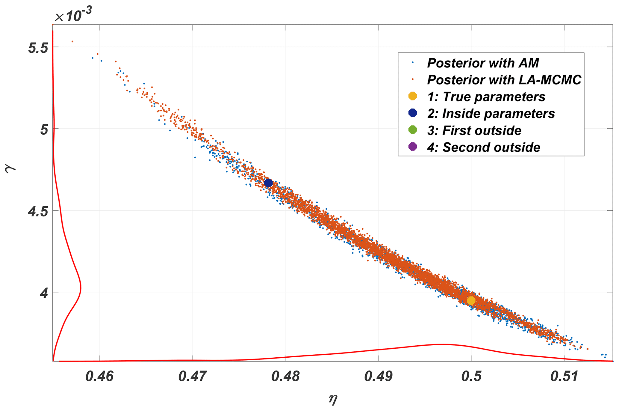
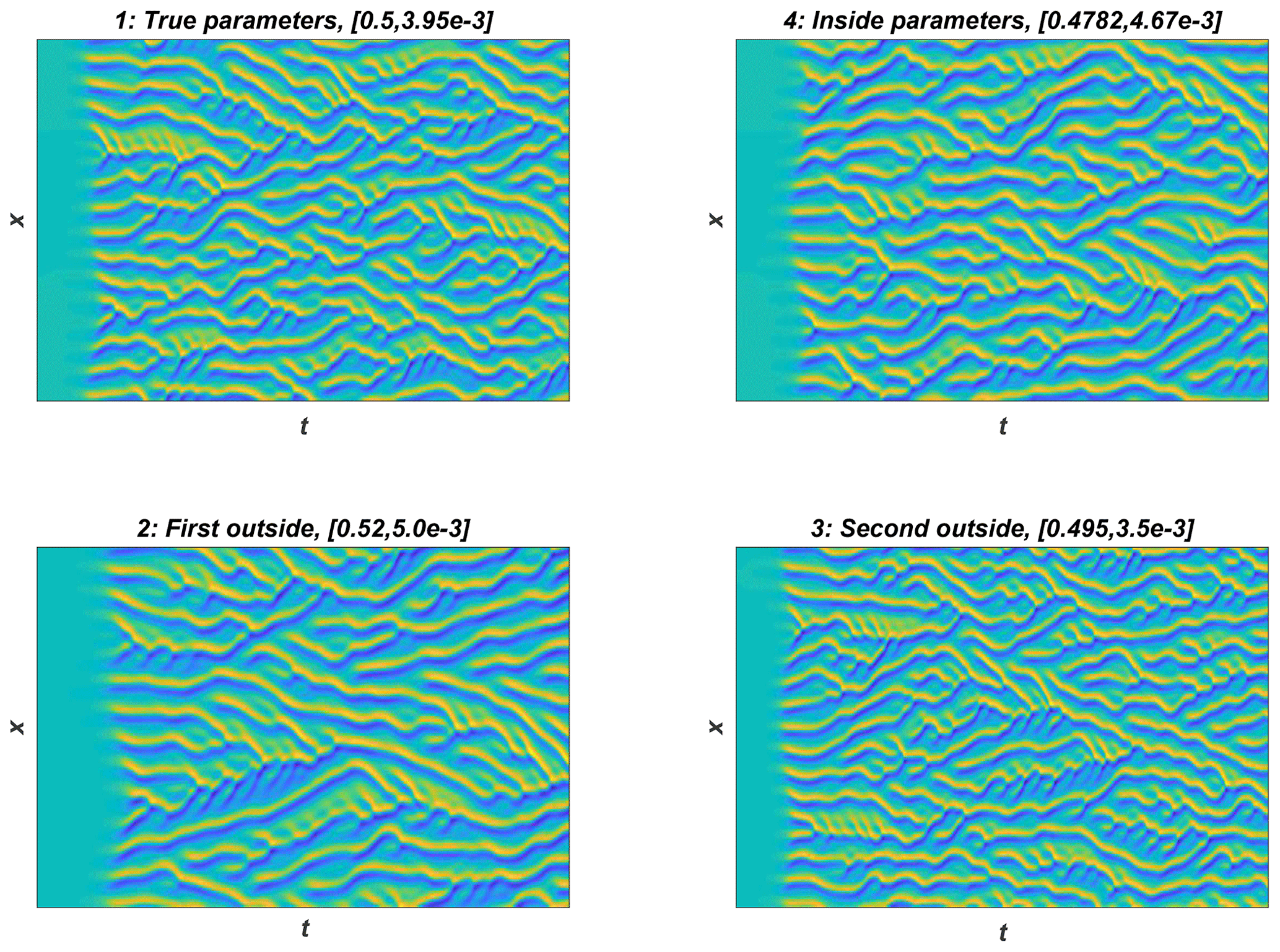
Figure 5Example model trajectories from the KS system. Panel (1) shows simulation using the true parameters, the parameters used for (4) are inside the posterior distribution, and (2) and (3) are generated from simulations with parameters outside the posterior distribution, shown in Fig. 4. The values of the parameter vectors 1, 2, 3, and 4 are given in Table 1. The y axis shows the 256-dimensional state vector, and the x axis the time evolution of the system.
Additional experiments were performed to evaluate the stability of the method when not all of the model states were observed. Keeping the setup otherwise fixed, the number of elements of the state vectors observed was reduced from the full 256 step by step to 128, 64, and 32. The resulting MCMC chains are presented in Fig. 6, and as expected, when less is observed, the size of the posterior distribution grows.

Figure 6Comparison between the KS system's posterior distribution in cases where all or only a part of the states are observed.
4.3 The quasi-geostrophic model
The methodology is here applied to a computationally intensive model, where a brute-force parameter posterior estimation would be too time consuming. We employ the well-known quasi-geostrophic model (Fandry and Leslie, 1984; Pedlosky, 1987) using a dense grid to achieve complex chaotic dynamics in high dimensions. The wall-clock time for one long-time forward model simulation is roughly 10 min, so a naïve calculation of a posterior sample of size 100 000 would take around 2 years. We demonstrate how the application of the methods verified in the two previous examples reduces this time to a few hours.
The QG model approximates the behavior on a latitudinal “stripe” at two given atmospheric heights, projected onto a two-layered cylinder. The model geometry implies periodic boundary conditions, seamlessly stitching together the extreme eastern and western parts of the rectangular spatial domain with coordinates x and y. For the northern and southern edges, user-specified time-independent Dirichlet boundary conditions are used. In addition to these conditions and the topographic constraints, the model parameters include the mean thicknesses of the two interacting atmospheric layers, denoted by H1 and H2. The QG model also accounts for the Coriolis force. An example of the two-layer geometry is presented in Fig. 7.
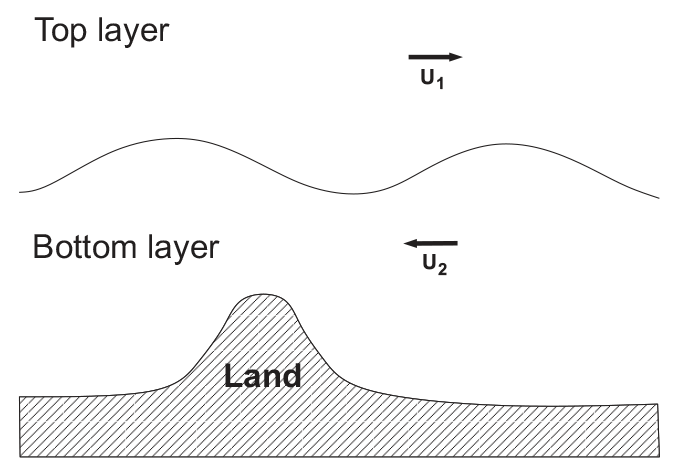
Figure 7An example of the layer structure of the two-layer quasi-geostrophic model. The terms U1 and U2 denote mean zonal flows, respectively, in the top and the bottom layer.
In a non-dimensional form, the QG system can be written as
where qi are potential vorticities, and ψi are stream functions with indexes for the upper and the lower layers, respectively. Both the qi and ψi are functions of time t and spatial coordinates x and y. The coefficients control how much the model layers interact, and gives a nondimensional version of β0, the northward gradient of the Coriolis force that gives rise to faster cyclonic flows closer to the poles. The Coriolis parameter is given by f0=2Wsin (ℓ), where W is the angular speed of Earth and ℓ is the latitude of interest. L and U give the length and speed scales, respectively, and is a gravity constant. Finally, defines the topography for the lower layer, where is the Rossby number of the system. For further details, see Fandry and Leslie (1984) and Pedlosky (1987).
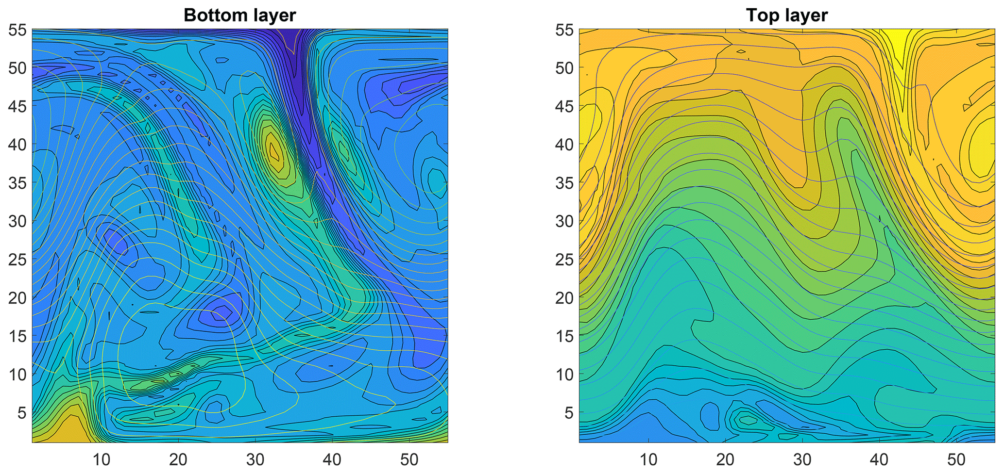
Figure 8An example of the 6050-dimensional state of the quasi-geostrophic model. The contour lines for both the stream function and potential vorticity are shown for both layers. Note the cylindrical boundary conditions.
It is assumed that the motion determined by the model is geostrophic, essentially meaning that potential vorticity of the flow is preserved on both layers:
Here, ui and vi are velocity fields, which are functions of both space and time. They are obtained from the stream functions ψi via
Equations (13)–(16) define the spatiotemporal evolution of the quantities qi,ψi, .
The numerical integration of this system is carried out using the semi-Lagrangian scheme, where the potential vorticities qi are computed according to Eq. (15) for given velocities ui and vi. With these qi the stream functions can then be obtained from Eqs. (13) and (14) with a two-stage finite difference scheme.
Finally, the velocity field is updated by Eq. (16) for the next iteration round.
For estimating model parameters from synthetic data, a reference data set is created with 64 epochs each containing N=1000 observations. These data are sampled from the model trajectory with Δt=8 (where a time step of length 1 corresponds to 6 h) in the time interval [192,8192], that amounts to a long-range integration of roughly 5–6 years of a climate model. The spatial domain is discretized into a 55×55 grid, which results in consistent chaotic behavior and more complex dynamics than with the often-used 20×40 grid. This is reflected in higher variability in the feature vectors, as seen in the Fig. 1. A snapshot of the 6050-dimensional trajectory of the QG system is displayed in Fig. 8.
The model state is characterized by two distinct fields, the vorticities and stream functions, that naturally are dependent on each other. As shown in (Haario et al., 2015), it is useful to construct separate feature vectors to characterize the dynamics in such situations. For this reason, two separate feature vectors are constructed – one for the potential vorticity on both layers and the other for the stream function.
The Gaussian likelihood of the state is created by stacking these two feature vectors one after another.
The normality of the resulting 2(M+1)-dimensional vector may again be verified as shown in Fig. 1. The number of bins was set to 32, leading to parameter values R0=55 and b=1.075 for potential vorticity, and R0=31, and b=1.046 for the stream function.
For parameter estimation, inferring the layer heights from synthetic data is considered. The reference data set with nepo=64 integrations is produced using the values H1=5500 and H2=4500. A single forward model evaluation takes 10 min on a fast laptop, and therefore generating MCMC chains of length 105 with brute force would take around 2 years to run. As previously, using LA-MCMC again reduces the computation time by a factor of 100.
In the experiments performed, the number of forward model evaluations needed was ranging in the interval [682,762], which translates to around 1 week of computing time. As verified with Kuramoto–Sivashinsky example, the forward model integration can be split to segments computed in parallel, which reduced time required to generate data for computing the likelihood further with a factor around 50, corresponding to around 3 h for generating the MCMC chain. The pairwise distances for generating the feature vectors were computed on a GPU, and therefore the required computation time for doing this was negligible compared to the model integration time. The posterior distribution of the two parameters is presented in Fig. 9.

Figure 9The clearly non-Gaussian posterior distribution of the H1 and H2 parameters of the quasi-geostrophic system shows how these parameters anticorrelate with each other.
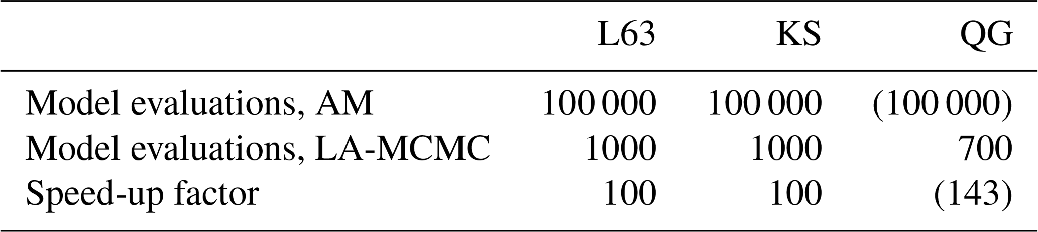
Bayesian parameter estimation with computationally demanding computer models is highly non-trivial. The associated computational challenges often become insurmountable when the model dynamics are chaotic. In this work, we showed it is possible to overcome these challenges by combining the CIL with an MCMC method based on local surrogates of the log-likelihood function (LA-MCMC). The CIL captures changes in the geometry of the underlying attractor of the chaotic system, while local approximation MCMC makes generating long MCMC chains based on this likelihood tractable, with computational savings of roughly 2 orders of magnitude, as shown in Table 2. Our methods were verified by sampling the parameter posteriors of the Lorenz 63 and the Kuramoto–Sivashinsky models, where an (expensive) comparison to exact MCMC with the CIL was still feasible. Then we applied our approach to the quasi-geostrophic model with a deliberately extended grid size. Without CIL, parameter estimation would not have been possible with chaotic models such as these; without LA-MCMC, the generation of long MCMC and sufficiently accurate chains for the higher-resolution QG model parameters would have been computationally intractable. We note that the computational demands of the QG model already get quite close to those of weather models at coarse resolutions. We believe that the approach developed here can provide ways to solve problems such as the climate model closure parameter estimation investigated in Järvinen et al. (2010) or long-time assimilation problems with uncertain model parameters, discussed in Rougier (2013) as unsolved and intractable.
Table 2Summary of results. This table shows the speed-up due to the CIL/LA-MCMC combination. Since running the quasi-geostrophic model 100 000 times was not possible, the nominal length of the MCMC chain and the speed-up due to LA-MCMC are reported in parentheses in the last column. The numbers of forward model evaluations with LA-MCMC (second row) are rough averages over several MCMC simulations.
There are many potential directions for extension of this work. First, it should be feasible to run parallel LA-MCMC chains that share model evaluations in a single evaluated set; doing so can accelerate the construction of accurate local surrogate models, as demonstrated in Conrad et al. (2018), and is a useful way of harnessing parallel computational resources within surrogate-based MCMC. Extending this approach to higher-dimensional parameters is also of interest. While LA-MCMC has been successfully applied to chains of dimension up to q=12 (Conrad et al., 2018), future work should explore sparsity and other truncations of the local polynomial approximation to improve scaling with dimension. From the CIL perspective, calibrating more complex models, such as weather models, often requires choosing the part of the state vector from which the feature vectors are computed. While computing the likelihood from the full high-dimensional state is computationally feasible, Haario et al. (2015) showed that carefully choosing a subset of the state for the feature vectors performs better. Also, the epochs may need to be chosen sufficiently long to include potential rare events, so that changes in rare event patterns can be identified. This, naturally, will increase the computational cost if one wants to be confident in the inclusion of such events.
While answering these questions will require further work, we believe the research presented in this paper provides a promising and reasonable step towards estimating parameters in the context of expensive operational models.
The MATLAB code that documents the CIL and LA-MCMC approaches is available in the Supplement. Forward model code for performing model simulations (Lorenz, Kuramoto–Sivashinsky, and quasi-geostrophic model) is also available in the Supplement.
The data were created using the code provided in the Supplement.
The supplement related to this article is available online at: https://doi.org/10.5194/gmd-14-4319-2021-supplement.
HH and YM designed the study with input from all authors. SS, HH, AD, and JS combined the CIL and LA-MCMC methods for carrying out the research. AB wrote and provided implementations of the KS and QG models for GPUs, including custom numerics and testing. SS wrote the CIL code and the version of LA-MCMC used (based on earlier work by Antti Solonen), and carried out the simulations. All authors discussed the results and shared the responsibility of writing the manuscript. SS prepared the figures.
The authors declare that they have no conflict of interest.
Publisher's note: Copernicus Publications remains neutral with regard to jurisdictional claims in published maps and institutional affiliations.
This work was supported by the Centre of Excellence of Inverse Modelling and Imaging (CoE), Academy of Finland, decision no. 312 122. Sebastian Springer was supported by the Academy of Finland, project no. 334 817. Youssef Marzouk and Andrew Davis were supported by the US Department of Energy, Office of Advanced Scientific Computing Research (ASCR), SciDAC program, as part of the FASTMath Institute.
This research has been supported by the Academy of Finland (grant no. 312122).
This paper was edited by Rohitash Chandra and reviewed by two anonymous referees.
Andrieu, C. and Roberts, G. O.: The pseudo-marginal approach for efficient Monte Carlo computations, Ann. Statist., 37, 697–725, https://doi.org/10.1214/07-AOS574, 2009. a, b
Asch, M., Bocquet, M., and Nodet, M.: Data Assimilation: Methods, Algorithms, and Applications, SIAM, Society for Industrial and Applied Mathematics, Philadelphia, PA, 2016. a
Beaumont, M. A., Zhang, W., and Balding, D. J.: Approximate Bayesian Computation in Population Genetics, Genetics, 162, 2025–2035, 2002. a
Borovkova, S., Burton, R., and Dehling, H.: Limit theorems for functionals of mixing processes with applications to U-statistics and dimension estimation, T. Am. Math. Soc., 353, 4261–4318, https://doi.org/10.1090/S0002-9947-01-02819-7, 2001. a
Cencini, M., Cecconi, F., and Vulpiani, A.: Chaos: From Simple Models to Complex Systems, World Scientific: Series on advances in statistical mechanics, WORLD SCIENTIFIC, https://doi.org/10.1142/7351, 2010. a
Conn, A. R., Scheinberg, K., and Vicente, L. N.: Introduction to derivative-free optimization, MPS-SIAM, Society for Industrial and Applied Mathematics, https://doi.org/10.1137/1.9780898718768, 2009. a
Conrad, P. R., Marzouk, Y. M., Pillai, N. S., and Smith, A.: Accelerating asymptotically exact MCMC for computationally intensive models via local approximations, J. Am. Stat. Assoc., 111, 1591–1607, https://doi.org/10.1080/01621459.2015.1096787, 2016. a, b, c, d, e, f, g, h, i
Conrad, P. R., Davis, A. D., Marzouk, Y. M., Pillai, N. S., and Smith, A.: Parallel local approximation MCMC for expensive models, SIAM/ASA Journal on Uncertainty Quantification, 6, 339–373, https://doi.org/10.1137/16M1084080, 2018. a, b, c, d, e, f
Davis, A., Marzouk, Y., Smith, A., and Pillai, N.: Rate-optimal refinement strategies for local approximation MCMC, arXiv, available at: https://arxiv.org/abs/2006.00032, arXiv:2006.00032, 2020. a, b, c, d, e, f, g, h, i, j, k
Davis, A. D.: Prediction under uncertainty: from models for marine-terminating glaciers to Bayesian computation, PhD thesis, Massachusetts Institute of Technology, Massachusetts, 2018. a, b, c
Donsker, M. D.: An invariance principle for certain probability limit theorems, Mem. Am. Math. Soc., 6, 1–10, 1951. a
Durbin, J. and Koopman, S. J.: Time Series Analysis by State Space Methods, Oxford University Press, Oxford, 2012. a
ECMWF: IFS Documentation – Cy40r1, Tech. Rep. 349, European Centre for Medium-Range Weather Forecasts, Reading, England, available at: https://www.ecmwf.int/sites/default/files/elibrary/2014/9203-part-iii-dynamics-and-numerical-procedures.pdf (last access: October 2020), 2013. a
Fandry, C. B. and Leslie, L. M.: A Two-Layer Quasi-Geostrophic Model of Summer Trough Formation in the Australian Subtropical Easterlies, J. Atmos. Sci., 41, 807–818, https://doi.org/10.1175/1520-0469(1984)041<0807:ATLQGM>2.0.CO;2, 1984. a, b
Gamerman, D.: Markov Chain Monte Carlo: Stochastic Simulation for Bayesian Inference, Chapman & Hall/CRC Texts in Statistical Science, Taylor & Francis, London, 1997. a
Gelman, A., Carlin, J., Stern, H., Dunson, D., Vehtari, A., and Rubin, D.: Bayesian Data Analysis, Chapman and Hall/CRC, 3rd edn., 2013. a, b
Grassberger, P. and Procaccia, I.: Procaccia, I.: Estimation of the Kolmogorov entropy from a chaotic signal, Phys. Rev. A, 28, 2591–2593, https://doi.org/10.1103/PhysRevA.28.2591, 1983a. a
Grassberger, P. and Procaccia, I.: Measuring the strangeness of strange attractors, Physica D, 9, 189–208, https://doi.org/10.1016/0167-2789(83)90298-1, 1983b. a
Haario, H., Saksman, E., and Tamminen, J.: An adaptive Metropolis algorithm, Bernoulli, 7, 223–242, 2001. a
Haario, H., Laine, M., Mira, A., and Saksman, E.: DRAM: Efficient adaptive MCMC, Stat. Comput., 16, 339–354, https://doi.org/10.1007/s11222-006-9438-0, 2006. a, b
Haario, H., Kalachev, L., and Hakkarainen, J.: Generalized correlation integral vectors: A distance concept for chaotic dynamical systems, Chaos, 25, 063102, https://doi.org/10.1063/1.4921939, 2015. a, b, c, d, e, f, g
Hakkarainen, J., Ilin, A., Solonen, A., Laine, M., Haario, H., Tamminen, J., Oja, E., and Järvinen, H.: On closure parameter estimation in chaotic systems, Nonlin. Processes Geophys., 19, 127–143, https://doi.org/10.5194/npg-19-127-2012, 2012. a
Hakkarainen, J., Solonen, A., Ilin, A., Susiluoto, J., Laine, M., Haario, H., and Järvinen, H.: A dilemma of the uniqueness of weather and climate model closure parameters, Tellus A, 65, 20147, https://doi.org/10.3402/tellusa.v65i0.20147, 2013. a
Houtekamer, P. L. and Zhang, F.: Review of the Ensemble Kalman Filter for Atmospheric Data Assimilation, Mon. Weather Rev., 144, 4489–4532, https://doi.org/10.1175/MWR-D-15-0440.1, 2016. a
Huttunen, J., Kaipio, J., and Haario, H.: Approximation error approach in spatiotemporally chaotic models with application to Kuramoto–Sivashinsky equation, Comput. Stat. Data Anal., 123, 13–31, https://doi.org/10.1016/j.csda.2018.01.015, 2018. a
Järvinen, H., Räisänen, P., Laine, M., Tamminen, J., Ilin, A., Oja, E., Solonen, A., and Haario, H.: Estimation of ECHAM5 climate model closure parameters with adaptive MCMC, Atmos. Chem. Phys., 10, 9993–10002, https://doi.org/10.5194/acp-10-9993-2010, 2010. a, b, c
Jarvinen, H., Laine, M., Solonen, A., and Haario, H.: Ensemble prediction and parameter estimation system: the concept, Q. J. Roy. Meteor. Soc., 138, 281–288, https://doi.org/10.1002/qj.923, 2011. a
Kennedy, M. C. and O'Hagan, A.: Bayesian calibration of computer models, J. R. Stat. Soc. B, 63, 425–464, https://doi.org/10.1111/1467-9868.00294, 2001. a
Kohler, M.: Universal consistency of local polynomial kernel regression estimates, Ann. I. Stat. Math., 54, 879–899, 2002. a, b
Kuramoto, Y.: Diffusion-Induced Chaos in Reaction Systems, Progress of Theoretical Physics Supplement, 64, 346–367, https://doi.org/10.1143/PTPS.64.346, 1978. a
Kuramoto, Y. and Yamada, T.: Turbulent State in Chemical Reactions, Prog. Theor. Phys., 56, 679–681, https://doi.org/10.1143/PTP.56.679, 1976. a
Laine, M., Solonen, A., Haario, H., and Jarvinen, H.: Ensemble prediction and parameter estimation system: the method, Q. J. Roy. Meteor. Soc., 138, 289–297, https://doi.org/10.1002/qj.922, 2011. a
Law, K., Stuart, A., and Zygalakis, K.: Data Assimilation, Springer International Publishing, Cham, Switzerland, 2015. a
Liu, J. and West, M.: Combined Parameter and State Estimation in Simulation-Based Filtering, Springer New York, New York, NY, 197–223, https://doi.org/10.1007/978-1-4757-3437-9_10, 2001. a
Lorenz, E. N.: Deterministic Nonperiodic Flow, J. Atmos. Sci., 20, 130–141, https://doi.org/10.1175/1520-0469(1963)020<0130:DNF>2.0.CO;2, 1963. a
Luego, D., Martino, L., Elvira, V., and Särkkä, S.: A survey of Monte Carlo methods for parameter estimation, EURASIP J. Adv. Sig. Pr., 2020, 25, https://doi.org/10.1186/s13634-020-00675-6, 2020. a
Morzfeld, M., Adams, J., Lunderman, S., and Orozco, R.: Feature-based data assimilation in geophysics, Nonlin. Processes Geophys., 25, 355–374, https://doi.org/10.5194/npg-25-355-2018, 2018. a, b
Neumeyer, N.: A central limit theorem for two-sample U-processes, Stat. Probabil. Lett., 67, 73–85, https://doi.org/10.1016/j.spl.2002.12.001, 2004. a
Ollinaho, P., Laine, M., Solonen, A., Haario, H., and Järvinen, H.: NWP model forecast skill optimization via closure parameter variations, Q. J. Roy. Meteor. Soc., 139, 1520–1532, https://doi.org/10.1002/qj.2044, 2012. a
Ollinaho, P., Bechtold, P., Leutbecher, M., Laine, M., Solonen, A., Haario, H., and Järvinen, H.: Parameter variations in prediction skill optimization at ECMWF, Nonlin. Processes Geophys., 20, 1001–1010, https://doi.org/10.5194/npg-20-1001-2013, 2013. a
Ollinaho, P., Järvinen, H., Bauer, P., Laine, M., Bechtold, P., Susiluoto, J., and Haario, H.: Optimization of NWP model closure parameters using total energy norm of forecast error as a target, Geosci. Model Dev., 7, 1889–1900, https://doi.org/10.5194/gmd-7-1889-2014, 2014. a
Pedlosky, J.: Geophysical Fluid Dynamics, Springer-Verlag, New York, 22–57, 1987. a, b
Price, L. F., Drovandi, C. C., Lee, A., and Nott, D. J.: Bayesian Synthetic Likelihood, J. Comput. Graph. Stat., 27, 1–11, https://doi.org/10.1080/10618600.2017.1302882, 2018. a, b
Robert, C. and Casella, G.: Monte Carlo Statistical Methods, Springer-Verlag, New York, 2004. a
Roeckner, E., Bäuml, G., Bonaventura, L., Brokopf, R., Esch, M., Giorgetta, M., Hagemann, S., Kirchner, I., Kornblueh, L., Manzini, E., Rhodin, A., Schlese, U., Schulzweida, U., and Tompkins, A.: The atmospheric general circulation model ECHAM 5. PART I: Model description, Report, MPI fur Meteorologie, Hamburg, 349, 2003. a
Rougier, J.: “Intractable and unsolved”: some thoughts on statistical data assimilation with uncertain static parameters, Philos. T. R. Soc. S.-A, 371, 371, https://doi.org/10.1098/rsta.2012.0297, 2013. a, b, c
Sacks, J., Welch, W. J., Mitchell, T. J., and Wynn, H. P.: Design and Analysis of Computer Experiments, Stat. Sci., 4, 409–423, 1989. a
Sivashinsky, G.: Nonlinear analysis of hydrodynamic instability in laminar flames – I. Derivation of basic equations, Acta Astronaut., 4, 1177–1206, https://doi.org/10.1016/0094-5765(77)90096-0, 1977. a
Solonen, A., Ollinaho, P., Laine, M., Haario, H., Tamminen, J., and Järvinen, H.: Efficient MCMC for Climate Model Parameter Estimation: Parallel Adaptive Chains and Early Rejection, Bayesian Anal., 7, 715–736, https://doi.org/10.1214/12-BA724, 2012. a
Springer, S., Haario, H., Shemyakin, V., Kalachev, L., and Shchepakin, D.: Robust parameter estimation of chaotic systems, Inv. Prob. Imag., 13, 1189–1212, https://doi.org/10.3934/ipi.2019053, 2019. a
Stevens, B., Giorgetta, M., Esch, M., Mauritsen, T., Crueger, T., Rast, S., Salzmann, M., Schmidt, H., Bader, J., Block, K., Brokopf, R., Fast, I., Kinne, S., Kornblueh, L., Lohmann, U., Pincus, R., Reichler, T., and Roeckner, E.: Atmospheric component of the MPI-M Earth System Model: ECHAM6, J. Adv. Model. Earth Sy., 5, 146–172, https://doi.org/10.1002/jame.20015, 2013. a
Tarantola, A.: Inverse Problem Theory and Methods for Model Parameter Estimation, Society for Industrial and Applied Mathematics, Philadelphia, 2005. a
Wood, S.: Statistical inference for noisy nonlinear ecological dynamic systems, Nature, 466, 1102–1104, 2010. a, b
Yiorgos Smyrlis, D. P.: Computational study of chaotic and ordered solutions of the Kuramoto-Shivashinsky equation, NASA Contractor Report 198283, 96-12, NASA reports, Hampton, Virginia, 1996. a