The ENEA-REG system (v1.0), a multi-component regional Earth system model: sensitivity to different atmospheric components over the Med-CORDEX (Coordinated Regional Climate Downscaling Experiment) region

In this study, a new regional Earth system model is developed and applied to the Med-CORDEX (Coordinated Regional Climate Downscaling Experiment) region. The ENEA-REG system is made up of two interchangeable regional climate models as atmospheric components (RegCM, REGional Climate Model, and WRF, Weather Research and Forecasting), a river model (Hydrological Discharge, HD), and an ocean model (Massachusetts Institute of Technology General Circulation Model, MITgcm); processes taking place at the land surface are represented within the atmospheric models with the possibility to use several land surface schemes of different complexity. The coupling between these components is performed through the RegESM driver.

Here, we present and describe our regional Earth system model and evaluate its components using a multidecadal hindcast simulation over the period 1980–2013 driven by ERA-Interim reanalysis. We show that the atmospheric components correctly reproduce both large-scale and local features of the Euro-Mediterranean climate, although we found some remarkable biases: in particular, WRF has a significant cold bias during winter over the northeastern bound of the domain and a warm bias in the whole continental Europe during summer, while RegCM overestimates the wind speed over the Mediterranean Sea.

Similarly, the ocean component correctly reproduces the analyzed ocean properties with performances comparable to the state-of-art coupled regional models contributing to the Med-CORDEX initiative.

Our regional Earth system model allows studying the Euro-Mediterranean climate system and can be applied to both hindcast and scenario simulations.

1 Introduction

The Mediterranean Basin is a complex region characterized by pronounced topography and a complex land–sea distribution, including many islands and several straits. These features generate intense local atmosphere–sea interactions leading to the formation of intense local winds, like mistral, Etesian and bora, which, in turn, dramatically affect the Mediterranean ocean circulation (e.g., Artale et al., 2010; Lebeaupin-Brossier et al., 2015; Turuncoglu and Sannino, 2017). Given the relatively fine spatial scales at which these processes occur, the Mediterranean Basin provides an excellent opportunity to study the regional climate, with a particular focus on the air–sea coupling (Sevault et al., 2014; Turuncoglu and Sannino, 2017). For these reasons, regional coupled models have been developed and used to study both present and future Mediterranean climate systems (e.g., Dubois et al., 2012; Ruti et al., 2016; Darmaraki et al., 2019; Parras-Berrocal et al., 2020); these models, depending on their complexity, include several physical components of the climate system, like atmosphere, ocean, land surface, rivers and biogeochemistry (both for land and ocean) (e.g., Drobinski et al., 2012; Sevault et al., 2014; Reale et al., 2020; Somot et al., 2008). Over the last 2 decades, an increasing number of studies have been performed over the Mediterranean Basin. Nowadays, there is a coordinated effort to produce hindcast and future simulations over this region using regional coupled climate models sharing some common protocols (Ruti et al., 2016). In particular, the Coordinated Regional Climate Downscaling Experiment (CORDEX) was designed to produce worldwide, high-resolution regional climate simulations through a coordinated experiment protocol ensuring that model simulations are carried out under similar conditions thus facilitating the analysis, intercomparison and synthesis of different simulations (Giorgi and Gutowski, 2015 and 2016). In the framework of the CORDEX program, regional climate model simulations dedicated to the Mediterranean area belong to the Med-CORDEX initiative (Ruti et al., 2016; Somot et al., 2018b).

From an atmospheric point of view, the Mediterranean region is a transition zone between arid subtropics and temperate midlatitudes, characterized by low annual precipitation totals and high interannual variability; during winter, rain is brought by midlatitude westerlies, while warm and dry summer results from the influence of subtropical remote forcing triggered by the Indian monsoon (Tuel and Eltahir, 2020). A number of model studies have indicated that the Mediterranean is expected to be one of the most prominent and vulnerable climate change “hotspots” in the world; in particular, a significant decline in the amount of precipitation is predicted by several models over the 21st century (Giorgi, 2006; Tuel and Eltahir, 2020).

Given the Mediterranean Basin's complexity and the strong air–sea feedback, high-resolution regional Earth system models are an optimal tool for accurate simulation of past, present and future climate over this region. This paper aims to present and evaluate the newly developed regional Earth system model ENEA-REG; in particular, we evaluate the ability of the ENEA-REG system to represent the present climate of the Mediterranean adequately by making a hindcast simulation using the ERA-Interim reanalysis as boundary conditions. The performances of individual model components are evaluated, comparing results with a wide range of observation-based datasets. Taking full advantage of the RegESM driver's potential (Turuncoglu, 2019), which allows us to build up in a modular way regional coupled models, the ENEA-REG is composed of two interchangeable regional climate models (RCMs) used as atmospheric components of the Earth system. Keeping the ocean and river components fixed, our model allows us to explore the sensitivity of the ocean model to different atmospheric forcings: specifically, with the direct comparison of simulations differing in the atmospheric component, we infer the impact of different modeling choices on both air–sea processes and, consequently, on the ocean dynamics.

Our results help to define possible future modeling strategies in the context of Med-CORDEX simulations. Besides, developing a modular regional Earth system model with interchangeable components allows defining the model to be used for a given application depending on the model's skills over the region of interest. This capability could be of particular interest for other CORDEX experiments, as it is well known that some parameterizations perform poorly locally or over some regions producing large local biases.

2 Model description

2.1 The RegESM coupler

The ENEA-REG regional Earth system model can include several model components (atmosphere, river routing, ocean, wave) to allow different modeling applications. For each simulation, the modeling system components can be easily enabled or disabled via the driver's configuration file. The modeling framework also supports plugging new Earth system sub-components (e.g., atmospheric chemistry, sea ice, ocean biogeochemistry) with minimal code changes through its simplified interface, which is called “cap”. The National United Operational Prediction Capability (NUOPC) cap is a Fortran module that serves as an interface to a model when it is used in a NUOPC-based coupled system; it is a small software layer that sits on top of a model code, making calls into it and exposing model data structures in a standard way (Turuncoglu, 2019).

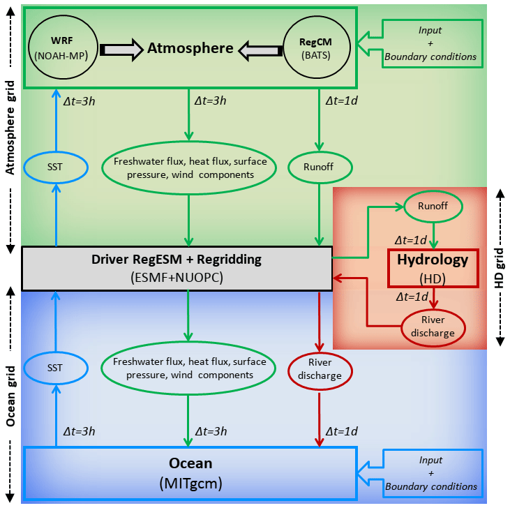
Figure 1 Schematic description of the ENEA-REG regional coupled model. The green block represents the atmosphere with the two components that can be selected and used (i.e., WRF and RegCM), the blue block is the ocean component (i.e., MITgcm), the red block represents the river routing component, and the gray block is the ESMF/NUOPC coupler, which collects, regrids and exchanges variables between the different components of the system.

In this study, the modeling system is configured to include three components: a regional atmospheric climate model, a regional ocean model and a hydrological model. The driver used to regrid and exchange data among the three components of the ENEA-REG modeling system is RegESM (Turuncoglu, 2019). The driver employs the Earth System Modeling Framework (ESMF) library (version 7.1) and the NUOPC layer to connect and synchronize each model component and perform interpolation among different horizontal grids (Turuncoglu, 2019). While the ESMF library deals with interpolation and regridding of exchanged fields, the NUOPC layer simplifies common tasks of model coupling like component synchronization and run sequence by providing an additional wrapper layer between coupled model and ESMF framework (Turuncoglu and Sannino, 2017; Turuncoglu, 2019). It also allows defining different coupling time intervals among the components to reproduce fast and slow interactions among the model components (Turuncoglu and Sannino, 2017; Turuncoglu, 2019). In this study, the model coupling time step between ocean and atmosphere is set to 3 h, while the coupling with the hydrological model is defined as 1 d. Also, the driver allows selecting the desired exchange fields from a simple field database containing all available variables that can be exported or imported by the different components. In this way, the coupled modeling system can be easily adapted depending on the application and the particular configuration of the experiment without any code customizations in both the driver and individual model components (Turuncoglu, 2019).

In the experiments presented here, the atmospheric model retrieves sea surface temperature (SST) from the ocean model (where grids are overlapped), while the ocean model collects surface pressure, wind components, freshwater (evaporation − precipitation, i.e., E−P) and heat fluxes from the atmospheric component. Similarly, the hydrological model uses surface and sub-surface runoff simulated by the atmospheric component to compute the river drainage and exchanges this field with the ocean component to close the water cycle. Further details on the ENEA-REG framework and the interaction among the components are schematically depicted in Fig. 1.

In the current work, we performed hindcast simulations covering the period 1 October 1979–31 December 2013.

2.2 The atmospheric components: WRF and RegCM

The ENEA-REG regional Earth system model is made up of two interchangeable atmospheric components: the Weather Research and Forecasting (WRF; Skamarock and Klemp, 2008) model and the REGional Climate Model (RegCM; Giorgi et al., 2012).

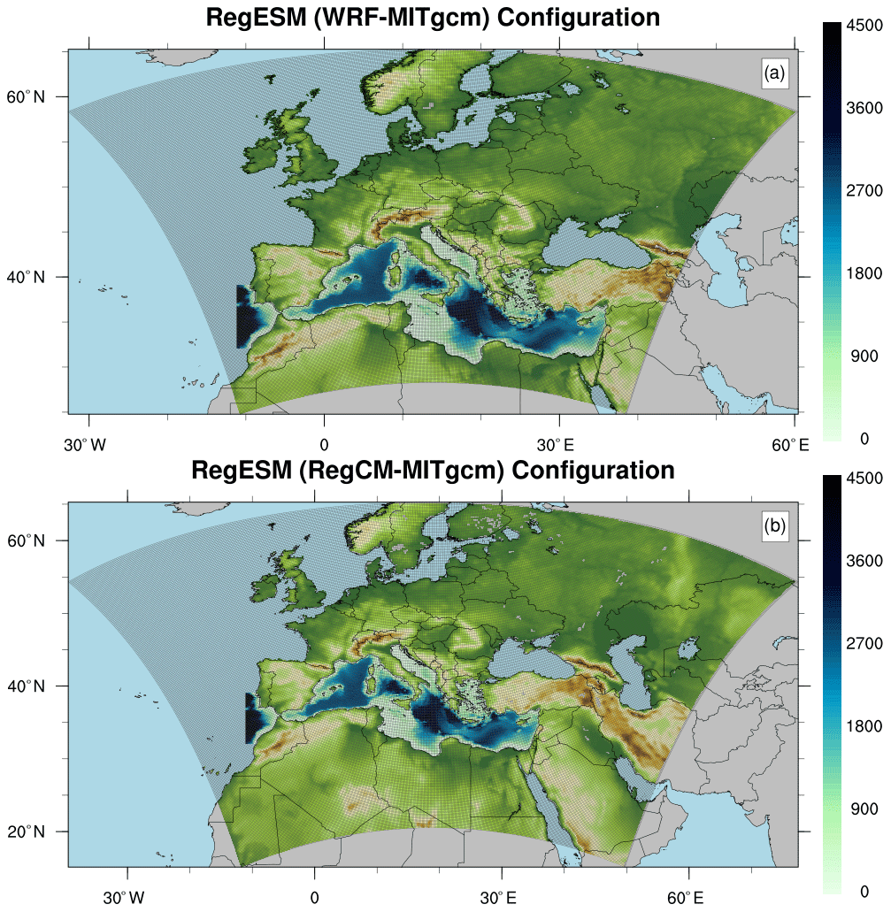
Figure 2 Different domains of the ENEA-REG system, with green shading representing the topography of the atmospheric models (i.e., WRF and RegCM; solid gray lines indicate the computational domain) and blue shading the bathymetry of the ocean component.

WRF is a limited-area, non-hydrostatic, terrain-following eta-coordinate mesoscale model developed by the NCAR/MMM (National Center for Atmospheric Research, Mesoscale and Microscale Meteorology division). WRF offers multiple options for various physical parameterizations; thus, it can be used for any region of the world for a wide range of applications ranging from operational forecasts to realistic and idealized dynamical studies. In this work, we use the dynamical core ARW (Advanced Research WRF, version 3.8.1) (Skamarock and Klemp, 2008), with a single-moment five-class scheme, to resolve the microphysics (Hong et al., 2004) and the Rapid Radiative Transfer Model for GCMs (RRTMG) for the shortwave and longwave radiation (Iacono et al., 2008). Convective precipitation and cumulus parameterization are resolved via the Kain–Fritsch scheme (Kain, 2004), and the planetary boundary layer (PBL) is represented through the Yongsei University scheme (Hong et al., 2006), while the exchange of heat, water and momentum between soil–vegetation and atmosphere is simulated by the Noah–MP land surface model (Niu et al., 2011). The model domain is projected on a Lambert conformal grid with a horizontal resolution of 15 km and with 35 vertical levels extending from land surface of up to 50 hPa (Fig. 2a). The initial and boundary meteorological conditions are provided by the European Centre for Medium-Range Weather Forecasts (ECMWF) reanalysis (Dee et al., 2011) with a horizontal resolution of 0.75^∘ every 6 h. The lateral buffer zone has a width of 10 grid points and uses an exponential relaxation to provide the model with lateral boundary conditions. A synthesis of parameterizations and input data used in this study is given in Table 1.

Table 1 Setup of atmospheric components of the ENEA-REG system with main physical parameterizations adopted in this study.

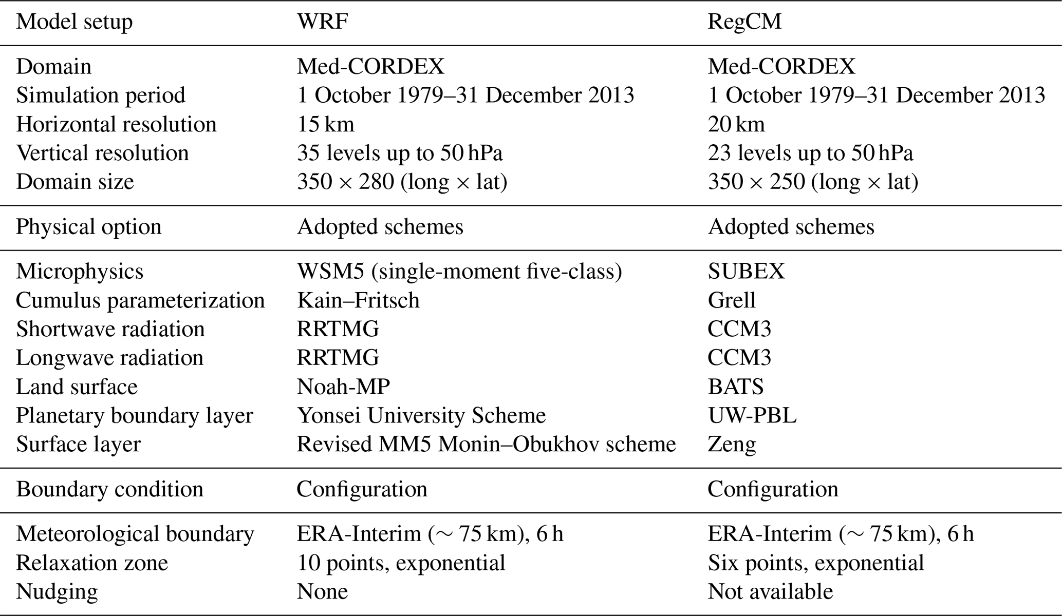
The other supported atmospheric component of the regional Earth system model is RegCM (version 4.5), a hydrostatic, compressible, sigma-p vertical coordinate model initially developed by Giorgi (1990) and Giorgi et al. (1993a, b) and then modified as discussed by Giorgi et al. (2012); RegCM is maintained by the International Centre for Theoretical Physics (ICTP)'s Earth System Physics (ESP) section. The dynamical core of RegCM is based on the primitive-equation, hydrostatic version of the National Center for Atmospheric Research (NCAR) and Pennsylvania State University mesoscale model MM5 (Grell et al., 1994). Similar to WRF, RegCM includes different physics and sub-grid parameterization options. In this study, radiation is simulated with the radiative transfer scheme of the global model CCM3 (Kiehl et al., 1996), cumulus convection is resolved through the Grell scheme (Grell, 1993) with a Fritsch–Chappell scheme for unresolved convection, the planetary boundary layer is represented via a modified version of the Holtslag parameterization (Giorgi et al., 2012), and the exchange of heat, water and momentum between soil–vegetation and atmosphere is simulated by the Biosphere-Atmosphere Transfer Scheme (BATS) (Dickinson et al., 1993). The resolved-scale precipitation is modeled with the SUBEX parameterization (Pal et al., 2000).

The model domain (Fig. 2b) is projected onto a Lambert conformal grid with a horizontal resolution of 20 km and with 23 vertical levels extending from the land surface of up to 50 hPa. Similarly to WRF, we used ERA-Interim data to force RegCM, and six grid points on each side are selected as a relaxation zone with an exponentially decreasing relaxation coefficient (Giorgi et al., 1993) (Table 1).

A few modifications have been made both in WRF and RegCM to receive the oceanic surface variables and send the atmospheric fields to the ocean component of the ENEA-REG system, as described in Fig. 1. Further details on the model's changes are described by Turuncoglu (2019).

2.3 The ocean component: MITgcm

The ocean component of the ENEA-REG system is the Massachusetts Institute of Technology General Circulation Model (MITgcm version c65; Marshall et al., 1997). The MITgcm solves both the hydrostatic and non-hydrostatic Navier–Stokes equations under the Boussinesq approximation for an incompressible fluid with a spatial finite-volume discretization on a curvilinear computational grid using the z^* rescaled height vertical coordinate (Adcroft and Campin, 2004). MITgcm is designed to run on different platforms, from scalar to high-performance computing (HPC) systems: it is parallelized via Message Passing Interface (MPI) through a horizontal domain decomposition technique.

A broad community of researchers uses MITgcm for a wide range of applications at various spatial and temporal scales ranging from local or regional (e.g., Sannino et al., 2009; Furue et al., 2015; Rosso et al., 2015; Sannino et al., 2015; McKiver et al., 2016; Sannino et al., 2017; Llasses et al., 2018; Peng et al., 2019) to global ocean simulations (e.g., Stammer et al., 2003; Forget et al., 2015; Breitkreuz et al., 2018; Forget and Ferreira, 2019). Moreover, MITgcm has also been used for climate studies coupled to the atmosphere (e.g., Artale et al., 2010; Polkova et al., 2014; Sitz et al., 2017; Sun et al., 2019).

In the configurations presented here, the MITgcm has been used in its hydrostatic, implicit free-surface, partial step topography formulation (Adcroft et al., 1997) and has already been customized and applied for simulating the Mediterranean circulation (Reale et al., 2020). The model domain has a horizontal resolution of $\mathrm{1}/\mathrm{12}$^∘, corresponding to 570 × 264 grid points, and covers the entire Mediterranean Sea with the boundary conditions in the Atlantic Ocean (Fig. 2). In the vertical, the model is discretized using 75 unevenly spaced Z levels going from 1 m at the surface to about 300 m in the deepest part of the basin. We use lateral open boundary conditions prescribed by the MITgcm Open Boundary Conditions (OBCS) package. Temperature and salinity boundary conditions in the Atlantic Ocean are interpolated from the global LEVITUS94 climatological monthly 3D data.

To ensure numerical stability, a sponge layer is added to the open boundary of the domain. Each variable is then relaxed toward the boundary values with a relaxation timescale that decreases linearly with distance from the boundary. The thickness of the sponge layer in terms of grid points is 18 and inner fields are relaxed toward boundary values using a 10 d period. Salinity and temperature fields in the Mediterranean Basin have been initialized using the MEDATLAS/2002 climatology for the month of October. This month corresponds to a situation of stable vertical stratification and can avoid sudden vertical mixing. A spin-up procedure for the ocean model has not been adopted. Usually, for climate studies, long spin-up is desirable to avoid the models drifting considerably from the initial conditions and tending to converge toward a new state given by the ocean physics (Sitz et al., 2017). However, since the main objective of this work is to compare the air–sea interaction simulated by two coupled regional models that share the same ocean model component, a long spin-up is not strictly necessary.

Similar to the atmospheric models, we have modified the MITgcm model in order to be forced by meteorological conditions derived by the atmospheric components of the ENEA-REG system (see Turuncoglu and Sannino 2017 for further details).

2.4 The river routing model: HD

The river discharge is a key variable in the Earth system modeling as it closes the water cycle between the atmosphere and ocean. The ENEA-REG system uses the Hydrological Discharge (HD, version 1.0.2) model, developed by the Max Planck Institute (Hagemann and Dümenil, 1997; Hagemann and Gates, 2001), to simulate freshwater fluxes over the land surface and to provide a river discharge to the ocean model. The HD model uses a regular global grid with a fixed horizontal resolution of 0.5^∘, and it is forced by daily surface runoff and drainage data. Similarly to other components, the HD model was slightly modified (Turuncoglu and Sannino, 2017) to retrieve surface runoff and drainage from the atmospheric components of the regional coupled model and to provide the river discharge to the ocean component (Fig. 1).

Although the HD model computes the discharge for each basin in the computational domain, a selection of the 18 main rivers has been given to the ocean model as boundary conditions. For instance, the Nile River has been prescribed as a climatological monthly mean because (1) the whole catchment basin is not covered by the domain of atmospheric models and (2) the natural discharge (which is the one computed by the model) is heavily modified by anthropic use and regulation. The river discharge data for the Nile is provided by the Global Runoff Data Centre (GRDC, Koblenz, Germany) as monthly means for the 1973–1984 periods. The same strategy has been used for the contribution coming from the Black Sea, namely, the monthly values of net flow have been taken from the study of the Black Sea water budget (Stanev et al., 2000).

3 Experiment design and observational datasets

In this work, we present Med-CORDEX hindcast climate simulations performed with the ENEA-REG model using both the atmospheric components of the system (i.e., WRF and RegCM). We perform the model validation over the period 1982–2013, using the first 2 years of simulation as spin-up to initialize all the fields of the different components of the coupled system. The validation of the coupled model focuses on sea surface temperature, sea surface salinity and mixed layer depth for the ocean and 2 m temperature, wind speed and freshwater and heat fluxes for the atmosphere. We also compare river discharge from the Po River as it influences the Adriatic Sea circulation and deep-water formation.

The simulated SST data are validated against the Objectively Interpolated Sea Surface Temperatures (OISST v2, Reynolds et al., 2002 and 2007), developed and distributed by the National Oceanic and Atmospheric Administration (NOAA). The OISST composites observations from different platforms (satellites, ships, buoys) on a $\mathrm{1}/\mathrm{4}$^∘ global grid and the gaps are filled by interpolation (Reynolds et al., 2007).

Salinity data for the Mediterranean Sea are obtained from MEDHYMAP (Jordà et al., 2017). For the mixed layer depth, we use a global climatology computed from more than 1 million Argo profiles collected from 2000 to the present (Holte et al., 2017); this climatology provides estimates of monthly mixed layer depth on a global 1^∘ gridded map.

As a reference dataset to evaluate the performances of the atmospheric components of the ENEA-REG system, we use ERA5: this allows us to test the model's ability to reliably reproduce their parent data (Mooney et al., 2013) and, unlike other observational data, this dataset provides information both on the area over land and over ocean. However, it should be considered that ERA5 has some weakness over the ocean and should be used cautiously (Belmonte Rivas and Stoffelen, 2019) to validate the wind speed over the Mediterranean Sea.

The observed river discharge of the Po River has been extracted from the series of measures at the Pontelagoscuro station from the RivDIS dataset (Vorosmarty et al., 1998).

4 Results

4.1 Evaluation of atmospheric models

The general ability of the atmospheric components of the ENEA-REG system to reproduce realistic spatiotemporal patterns of the most relevant physical variables is assessed by comparing model simulations with ERA5 during winter (DJF) and summer (JJA) seasons averaged over the reference period 1982–2013. In the present analysis, in addition to spatial patterns and anomalies maps, we also compute uncentered correlation patterns and domain-averaged bias to provide a measure of the model's skills.

Figure 3 Seasonal winter (DJF) and summer (JJA) spatial pattern (upper three rows) and bias (lower two rows) of 2 m air temperature as simulated by the coupled model using the two atmospheric components (i.e., WRF and RegCM) and the ERA5 dataset between 1982 and 2013. Note that in the bias rows ERA5 data are interpolated into the atmospheric model grid. Also note the differences in color scales between DJF and JJA climatologies.

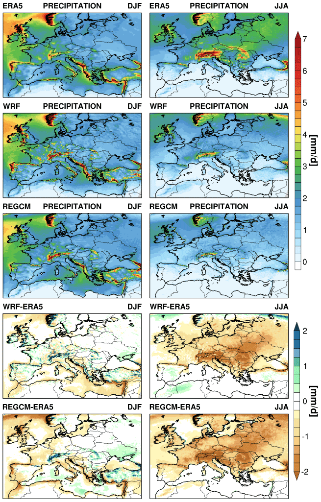
Figure 4 Seasonal winter (DJF) and summer (JJA) spatial pattern (upper three rows) and bias (lower two rows) of precipitation as simulated by the coupled model using the two atmospheric components (i.e., WRF and RegCM) and the ERA5 dataset between 1982 and 2013. Note that in the bias rows ERA5 data are interpolated into the atmospheric model grid.

Looking at the surface air temperature (Fig. 3), consistent with ERA5 data, during winter, both WRF and RegCM show a typical eastward gradient with temperature decreasing with increasing continentally, while during summer, the models correctly reproduce the decreasing south–north gradient with colder areas localized over mountainous regions (i.e., the Alps and Pyrenees). Looking at the anomalies, WRF shows a remarkable cold bias during DJF over northeastern Europe, with magnitudes larger than 4 ^∘C. Such a cold bias over this region has already been described in several studies, and it mainly depends on the poor representation of the snow–atmosphere interaction, amplified by the albedo feedback (e.g., Mooney et al., 2013; Kotlarski et al., 2014; García-Díez et al., 2015; Katragkou et al., 2015). Despite the fact that, when setting up WRF, we were aware of both the need to carefully select parameterization combinations and the issues associated with some of the selected parameterizations, we chose the present settings as they reproduce wind fields over the Mediterranean region well, which is relevant when running WRF coupled with an ocean model. Besides, as demonstrated by Mooney et al. (2013) in a sensitivity study, where different WRF physical parameterizations schemes were used to represent radiation, microphysics, convection, PBL and land surface over a large domain, no single combination of parameterizations yields optimal results. Unlike WRF, RegCM does not show any remarkable bias during winter and, in general, it shows a cold bias ranging between 1 and 2 ^∘C over the whole Mediterranean region. The good spatial agreement found during DJF between the simulated surface air temperature and the reference data is confirmed by the high spatial correlation varying between 0.97 in the case of WRF to 0.99 for RegCM, while the domain-averaged bias ranges from −1.4 for WRF to −0.15 ^∘C for RegCM.

During summer, both WRF and RegCM show a similar bias pattern over land, with a warm bias extending from France to eastern Europe and reaching magnitudes of up to 4 ^∘C in the case of WRF. In contrast, over the Mediterranean Sea, the two configurations show an opposite bias pattern, with WRF exhibiting a warm bias over the sea and RegCM a cold bias. In the case of WRF, the warm bias over land has already been described by Mooney et al. (2013), who showed how the selection of the land surface model mostly controls the simulated summer surface air temperature. Considering RegCM, our results are consistent with Turuncoglu and Sannino (2017), who described a similar behavior running RegCM both offline and coupled to the Regional Ocean Modeling System (ROMS) ocean model, with a temperature overestimation of up to 2.0–2.5 ^∘C during the summer season in central and eastern Europe. Overall, our regional models reproduce the observed spatial pattern well, the spatial correlation being larger than 0.99 for both WRF and RegCM. Because of compensation between warm bias over land and cold bias over the sea, during JJA, the configuration using RegCM shows a lower bias (0.14 ^∘C) than WRF (0.85 ^∘C).

Looking at precipitation, during winter, both the ENEA-REG configurations agree with ERA5 data, namely the atmospheric components can reproduce the major precipitation maxima over the Alps, the Balkans and western Norway with only a substantial local dry bias in the areas around the coastlines of the eastern Mediterranean. In contrast, during summer, WRF and RegCM systematically simulate less precipitation over most of continental Europe, with RegCM showing the largest dry bias (Fig. 4). Interestingly, considering WRF, these results are not consistent with Mooney et al. (2013), who reported a positive bias in mean daily precipitation over Europe during summer and related this wet bias to the land surface scheme used and partially to the microphysics scheme. However, Kotlarski et al. (2014) comparing three WRF experiments showed a different sensitivity, with two simulations overestimating mean summer precipitation and one underestimating it; they conclude that this result depends on the choice of different microphysics schemes. On the other side, Turuncoglu and Sannino (2017) found a similar bias pattern for RegCM during summer.

In general, the spatial performances of the ENEA-REG system are better when WRF is used as the atmospheric component: the spatial correlation ranges between 0.97 during DJF to 0.92 during JJA, while the configuration with RegCM exhibits a slightly lower pattern correlation (0.95 for DJF, 0.92 during JJA). Similarly, WRF has a smaller bias both during winter (−0.18 vs. −0.24 mm/d) and summer (−0.32 vs. −0.54 mm/d).

Despite the weak summer dry bias, the two atmospheric models reproduce precipitation over the sea well, enhancing the reliability of freshwater flux exchanged with the ocean component of the ENEA-REG system. Nevertheless, it should be noted that in the framework of coupled ocean–atmosphere models, the water budget (defined as evaporation − precipitation (E−P)) plays a pivotal role in the dynamics of the ocean component. For this reason, in Fig. 5 we show both the simulated interannual variability and mean seasonal cycle of the area-averaged Mediterranean Sea precipitation, evaporation along with their difference (i.e., E−P). Looking at precipitation, WRF shows a systematic dry bias over the Mediterranean Sea with respect to ERA5, while RegCM is in good agreement with the reference value. The mean annual cycles suggest that WRF underestimates rainfall during colder months (from October to April), while RegCM reproduces the observed seasonal cycle well, with a weak overestimation between August and October. Overall, the two configurations of the ENEA-REG system reproduce the seasonal cycle well, characterized by maximum values during fall and winter and a minimum in summer.

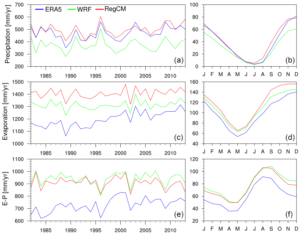
Figure 5 Interannual variability (a, c, e) and mean seasonal cycle (b, d, f, units mm/month) of freshwater flux components. i.e., precipitation (P), evaporation (E) and their difference (E−P), computed over the Mediterranean Basin as simulated by the ENEA-REG system and the ERA5 reanalysis.

The total simulated precipitation over the Mediterranean Sea is 372 ± 47 mm/yr using WRF and 496 ± 48 mm/yr in the case of RegCM, while ERA5 predicts 469 ± 50 mm/yr. In general, these estimates agree with previous studies: in particular, in a different experiment, where WRF was coupled with the Nucleus for European Modelling of the Ocean (NEMO) ocean model, Lebeaupin-Brossier et al. (2015) found a precipitation budget of 482 ± 53 mm/yr over the period 1989–2008, concluding that this value is in the upper part of the range given in the literature (290–510 mm/yr) (Mariotti et al., 2002; Pettenuzzo et al., 2010; Romanou et al., 2010; Criado-Aldeanueva et al., 2012). Similarly, in a regional climate system model developed over the Mediterranean Sea, where RegCM was coupled with the ROMS ocean model, Turuncoglu and Sannino (2017) found mean annual precipitation of 561 mm/yr during the period 1988–2006. In a different configuration, where the Aire Limitée Adaptation dynamique Développement InterNational (ALADIN) climate model was coupled with the NEMO ocean model, Sevault et al. (2014) found precipitation of 510 mm/yr over the period 1980–2012, while Sanchez-Gomez et al. (2011) compared 12 regional climate models finding a large spread among models with mean annual precipitation estimates ranging between 347 and 606 mm/yr with a mean value of 442 ± 84 mm/yr.

Compared to ERA5, the evaporation is systematically overestimated by both RegCM and WRF during our study period, although the year-to-year variability is reproduced well and the mismatch decreases with time (Fig. 5). Nevertheless, the two configurations correctly reproduce the seasonal cycle, characterized by an evaporation minimum in May and maxima during late summer and winter months, when the gradient between air–sea temperature is high, and the wind speed is strong. The total evaporation over the Mediterranean Sea is 1312 ± 34 mm/yr and 1405 ± 38 for WRF and RegCM, respectively, while ERA5 has lower evaporation of 1198 ± 59 mm/yr. Consistent with precipitation, our estimates agree well with previous studies: Lebeaupin-Brossier et al. (2015) using WRF coupled to NEMO found total evaporation of 1442 ± 45 mm/yr during the 1989–2008 period, while Turuncoglu and Sannino (2017) using RegCM coupled to ROMS reported a value of 1388 mm/yr during the 1988–2006 period. Sevault et al. (2014) estimated a mean annual evaporation of 1390 mm/yr, while Sanchez-Gomez et al. (2011) displayed a large variability among 12 regional climate models, with annual mean estimates ranging between 1066 and 1618 mm/yr, the latter using RegCM offline forced by ERA40 data. The comparison with previous studies highlights a general tendency of RegCM to overestimate the evaporation over the Mediterranean Sea, irrespective of the forcing data and parameterizations selected; this could likely be caused by an overestimation of wind speed (discussed later).

Interestingly, because of bias compensation WRF and RegCM show a similar E−P estimate (Fig. 5); however, in both the configurations of the ENEA-REG system we found a remarkable bias in E−P, with values larger than 100 mm/yr, which could significantly affect the ocean component. In any case, in both the ENEA-REG configurations, the monthly distribution of E–P shows a similar monthly distribution compared to the ERA5 dataset with a peak in the late summer caused by sparse precipitation and high evaporation. The total E−P estimated simulated using WRF is 940 ± 48 mm/yr while with RegCM we obtain a mean annual estimate of 909 ± 45 mm/yr; in contrast, ERA5 data have a lower E−P of 729 ± 56 mm/yr.

In addition to freshwater flux, wind speed is also a key variable for ocean models as it controls the evaporation over the sea surface and affects the ocean circulation through drag stress. Figure 6 shows the near-surface wind speed as simulated by the ENEA-REG system and ERA5 reanalysis. The comparison with the observationally based dataset indicates that both WRF and RegCM overestimate the wind speed over land during the two analyzed seasons, while over sea the atmospheric models are able to correctly simulate the wind speed, especially over the Gulf of Lion and the Aegean Sea, where the structure and magnitude of dominant mistral and Etesian winds are reproduced well by the models, although they produce too weak an Etesian during summer.

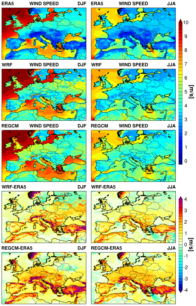
Figure 6 Seasonal winter (DJF) and summer (JJA) spatial pattern (upper three rows) and bias (lower two rows) of 10 m wind speed as simulated by the coupled model using the two atmospheric components (i.e., WRF and RegCM) and the ERA5 dataset between 1982 and 2013. Note that in the bias rows ERA5 data are interpolated into the atmospheric model grid.

It should also be noted that the large bias found over mountainous regions is an artifact due to the spatial resolution differences, with ERA5 reanalysis reproducing lower wind speed than both WRF and RegCM because of its coarser resolution. In general, the two atmospheric models have comparable performances in reproducing the observed spatial pattern; we find a correlation of 0.98 for both models and seasons, except for RegCM during summer (0.97). In contrast, WRF has a lower bias (0.7 m/s for DJF and 0.47 m/s for JJA) than RegCM (0.9 m/s for DJF and 0.7 m/s for JJA).

Besides freshwater flux and wind components, the surface net heat flux is used to drive the ocean model of the ENEA-REG system (Fig. 1); this variable represents the energy that the ocean surface receives from the atmosphere and is computed from net longwave, net shortwave, latent heat and sensible heat fluxes. In Fig. 7, we compare the simulated net energy flux with ERA5 data; overall, the two atmospheric models are in good agreement with the reference dataset during the analyzed seasons, although large biases are evident in both the atmospheric components. The models show similar skills in reproducing the ERA5 spatial patterns, both having a correlation of 0.96 during DJF, while in JJA RegCM (0.97) is slightly better than WRF (0.96). Similarly, RegCM also exhibits the lowest bias during both DJF (−1.3 W/m² vs. 5.7 W/m²) and JJA (3.1 W/m² vs. 13.8 W/m²). Looking at the spatial bias in more details, WRF shows a systematic positive bias over the land surface of up to 15 W/m² during winter and 20 W/m² in summer, while RegCM matches ERA5 data in DJF well with a bias lower than 5 W/m² but with a systematic negative bias (−10 W/m²) over the land during JJA.

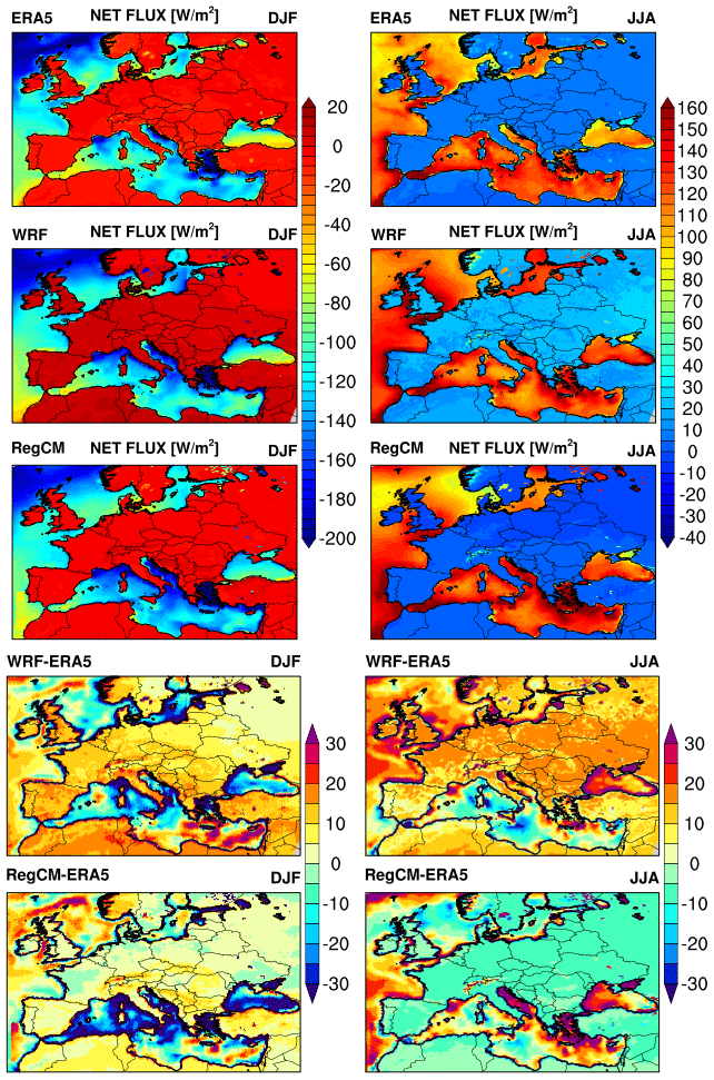
Figure 7 Seasonal winter (DJF) and summer (JJA) spatial pattern (upper three rows) and bias (lower two rows) of net heat flux as simulated by the coupled model using the two atmospheric components (i.e., WRF and RegCM) and the ERA5 dataset between 1982 and 2013. Note that ERA5 data are interpolated into atmospheric model grids for comparison purposes. Also note the differences in color scales between DJF and JJA climatologies.

Figure 8 Mean seasonal cycle of net heat flux components over the Mediterranean Basin as simulated by the ENEA-REG system and the ERA5 reanalysis over the period 1982–2013.

Figure 8 compares the monthly climatology of energy flux components averaged over the whole Mediterranean Sea with ERA5 data. The analysis of model results suggests that the atmospheric components systematically overestimate the latent heat during the whole year (Fig. 8a). The annual mean estimates are 104 ± 2.7 W/m² from WRF and 112 ± 2.9 W/m² from RegCM, with ERA5 showing a slightly smaller flux (95 ± 4.7 W/m²). This result is consistent with previous findings, namely, the overly intense wind speed simulated by WRF and RegCM over sea surface leads to large latent heat flux and consequently an overproduction of evaporative flux. We stress that our results are also consistent with previous studies; in particular, Turuncoglu and Sannino (2017) reported a value of 110.52 W/m² from RegCM coupled to ROMS, whilst Sanchez-Gomez et al. (2011) showed a value of 128 ± 5 W/m²; in this latter study, RegCM showed the largest overestimation of latent heat flux among 12 regional climate models.

The sensible heat flux shows similar behavior to that observed for the latent heat, namely, RegCM systematically overestimates this variable during the whole year, whilst WRF is closer to the reference data (Fig. 8b). The annual mean estimates are 12.9 ± 1.3 W/m² from WRF and 17.6 ± 1.2 W/m² from RegCM, while ERA5 has a slighter lower flux of 11.9 ± 1.1 W/m². Interestingly, using RegCM coupled to ROMS, Turuncoglu and Sannino (2017) found a smaller sensible heat flux of 9.85 W/m², while Sanchez-Gomez et al. (2011) running RegCM offline reported a value closer to our estimate (22 ± 2 W/m²); as the sensible heat strictly depends on the gradient between SST and air temperature the lower value of Turuncoglu and Sannino (2017) could be explained by a large discrepancy between the SSTs simulated by the MITgcm and the ROMS ocean models.

The mean annual cycle of net shortwave radiation is simulated well by the atmospheric models, with WRF showing an almost perfect match compared to ERA5, while RegCM underestimates the summer peak of about 25 W/m² and slightly overestimates the amount of radiation received by the ocean from January to April (Fig. 8c). The mean annual estimates are 200 ± 1.1 W/m² from WRF, 201 ± 1.2 W/m² form RegCM and 198 ± 1.1 W/m² from ERA5; for both the ENEA-REG configurations, these estimates are in agreement with other studies (Sanchez-Gomez et al., 2011; Turuncoglu and Sannino, 2017).

Comparison between simulated net longwave radiation and ERA5 shows that RegCM underestimates the thermal radiation during the whole year, while WRF generally agrees with ERA5 during cold months but largely underestimates the longwave radiation between March and October (Fig. 8d). In addition, the amplitude of seasonal variation is captured well by RegCM; in contrast, WRF shows a stronger month-to-month variability. The mean annual net longwave radiation simulated by RegCM and WRF is −77.6 ± 1.3 W/m² and −79.9 ± 1.2 W/m², respectively, while the ERA5 dataset predicts −84.8 ± 1.2 W/m².

4.2 Evaluation of ocean model

4.2.1 Surface processes

The correct representation of physical processes taking place at the air–sea interface is crucial for the success of a coupled climate simulation. A first evaluation of the goodness with which these processes are simulated is given by the analysis of the ocean surface variables like sea surface temperature (SST) and sea surface salinity (SSS).

Figure 9 shows the comparison of simulated SST with OISST reference data. We recall that SST, in a coupled simulation, is actually the same variable for ocean and atmosphere components (where grids overlap) and guides the thermal exchange providing active feedback among the two components: the higher the difference among SST and atmosphere temperature is, the larger the heat exchange at the interface will be that tends to lower such difference. Looking at Fig. 9, the coupled model reproduces the OISST spatial pattern well for both the configurations and seasons: WRF–MITgcm shows a mean bias of −0.5 ^∘C during winter and of 0.7 ^∘C during summer, while RegCM–MITgcm has a general negative bias in winter with a mean value of −0.9 ^∘C and a small positive bias in summer of 0.25 ^∘C. The large winter bias of the RegCM simulation is due to an important bias located in the Levantine Sea, while, during summer, WRF shows a large bias covering all the western basin and part of the Ionian Sea.

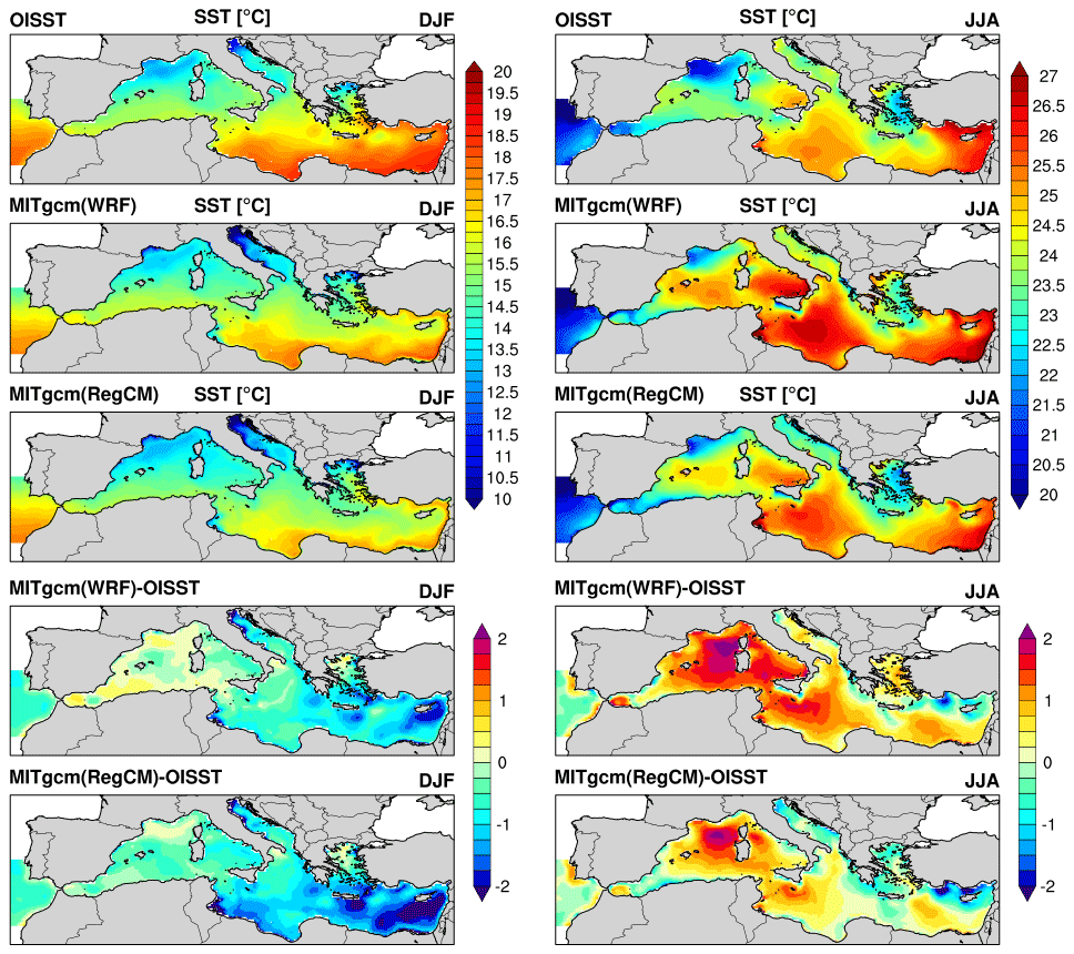
Figure 9 Seasonal winter (DJF) and summer (JJA) spatial pattern (upper three rows) and bias (lower two rows) of sea surface temperature (SST [^∘C]) as simulated by the coupled model using the two atmospheric components as forcing (i.e., WRF and RegCM) and OISST dataset between 1982 and 2013. Note that OISST data are interpolated into an ocean model grid for comparison purposes. Also note the differences in color scales between DJF and JJA climatologies.

In spite of some large local bias, the MITgcm, in both its configurations, reproduces well the observed interannual variability, although it has an overly marked year-to-year variability (Fig. 10a). The SST seasonal cycle closely follows the reference dataset, although both WRF–MITgcm and RegCM–MITgcm show a notable SST underestimation between October and April and a slight overestimation during summer months (Fig. 10b). Compared to similar modeling experiments, we note that an overall cold bias is not unusual in coupled simulations of the Mediterranean Sea, and the magnitude of the biases obtained in the present study is comparable to the literature (Sevault et al., 2014; Turuncoglu and Sannino, 2017; Reale et al., 2020). In particular, the seasonal spatial patterns in winter and summer closely resemble those shown in Turuncoglu and Sannino (2017), although they used the ROMS model to simulate the Mediterranean Sea. More recently, Reale et al. (2020) obtained a reduced cold bias with respect to both the available literature and the present experiment performed with RegCM–MITgcm; however a direct comparison is not straightforward as their simulation period was limited to the years 1994–2006.

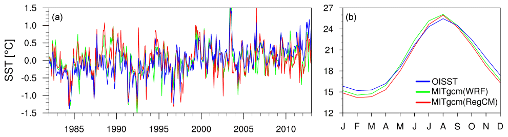
Figure 10 Comparison of monthly anomalies (a) and mean seasonal cycles (b) of sea surface temperature simulated by the ENEA-REG system with OISST observation.

Considering the SSS, compared to the reference data, both the simulations show very similar spatial patterns and biases (Fig. 11); the ocean model, in both its configurations, is saltier than the reference dataset, especially in the Adriatic Sea during summer. This is due to the fact that the Adriatic Sea is a dilution basin, mainly because of the important freshwater supply provided by rivers. In both the simulations the freshwater input from river runoff is heavily underestimated by the interactive river routing model (Fig. 12); this underestimation is slightly more evident in RegCM, which shows a lower river baseline with respect to WRF (Fig. 12).

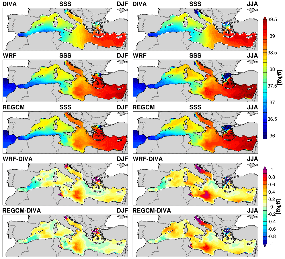
Figure 11 Seasonal winter (DJF) and summer (JJA) spatial pattern (upper three rows) and bias (lower two rows) of sea surface salinity (SSS [g/kg]) as simulated by the coupled model using the two atmospheric components (i.e., WRF and RegCM) and the MEDHYMAP dataset between 1982 and 2013. Note that MEDHYMAP data are interpolated into an ocean model grid for comparison purposes.

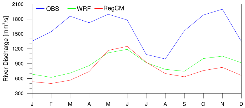
Figure 12 Mean seasonal cycle of the river discharge of the Po River into the Adriatic Sea as simulated by the two configurations of the coupled model and the observational dataset RivDIS.

Looking at the monthly SSS anomalies (Fig. 13a) we found a similar temporal variability compared to the reference data. Besides, the two configurations of the coupled model agree reasonably well, with the exception of 1996, when WRF has a remarkable drop in SSS due to the minimum in the freshwater flux (Fig. 5) caused by exceptional precipitation and river runoff during that year; interestingly, such a drop is also evident in other observational datasets (Sevault et al., 2014).

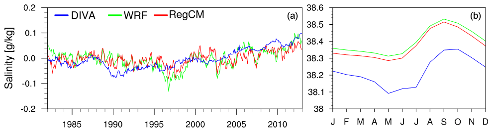
Figure 13 Comparison of monthly anomalies (a) and mean seasonal cycles (b) of sea surface salinity simulated by the ENEA-REG system with the MEDHYMAP dataset.

The seasonal cycle of SSS for the two simulations is very close during all the months (Fig. 13b). Compared to other studies, the mean bias of both WRF–MITgcm and RegCM–MITgcm is lower than that of similar simulations for the Mediterranean Sea as it does not exceed 0.1 g/km on a basin mean (e.g., Sevault et al., 2014; Turuncoglu and Sannino, 2017).

4.2.2 Sea surface height and circulation

The Strait of Gibraltar is the only connection between the Mediterranean Basin and the Atlantic Ocean. In general, the two-way exchange at the strait is constituted by an upper inflow of Atlantic water and a lower outflow of relatively colder and saltier Mediterranean water. However, the semidiurnal tidal effect is strong enough to reverse the direction of the flows during part of the tidal cycle. As this exchange represents the main driver of the circulation in the basin, the challenge of estimating its value has been faced for decades.

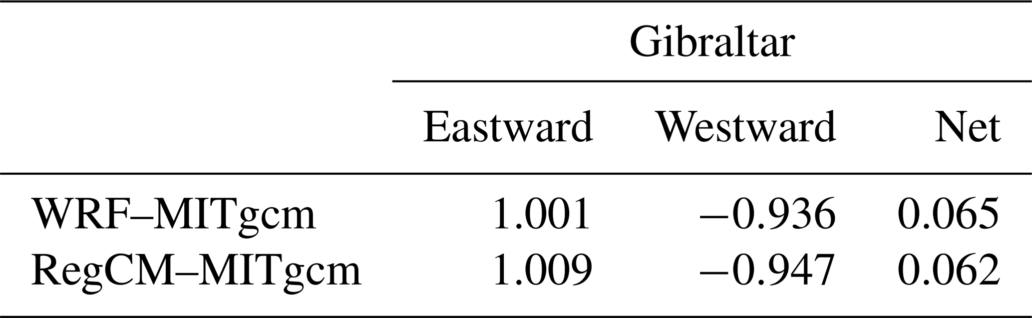
The inflow transport derived from the two coupled simulations is about 1 Sv (Table 2); similarly, the models predict a net transport of 0.06 Sv. Unfortunately, the estimate of the transport obtained from the direct measurements of velocities is affected by the limited number of moorings used to this purpose that cannot resolve the structure of the entire section. Therefore, some numerical models have also been used to reproduce and quantify the two-way exchange. Estimates of mean inflow range from about 0.72 Sv of Bryden et al. (1994) to 1.68 Sv of Bethoux (1979). Sannino et al. (2009) computed an inflow of 1.03 Sv using a three-dimensional numerical model characterized by a very high resolution in the strait. Similarly, the long-term net transport that balances the excess of evaporation over precipitation and river runoff in the Mediterranean has a value of about 0.05 Sv (Bryden et al., 1994; Sannino et al., 2009); it is noteworthy that our results agree well with these estimates (Table 2).

Table 2 Mean annual water transport (in Sv) through the Gibraltar Strait over the period 1982–2013.

The mean annual current velocity at 30 m depth and the mean annual sea surface height (SSH) are analyzed in Fig. 14 for WRF–MITgcm (a) and RegCM–MITgcm (b), respectively. The two simulations depict a similar mean annual circulation, with similar large-scale features.

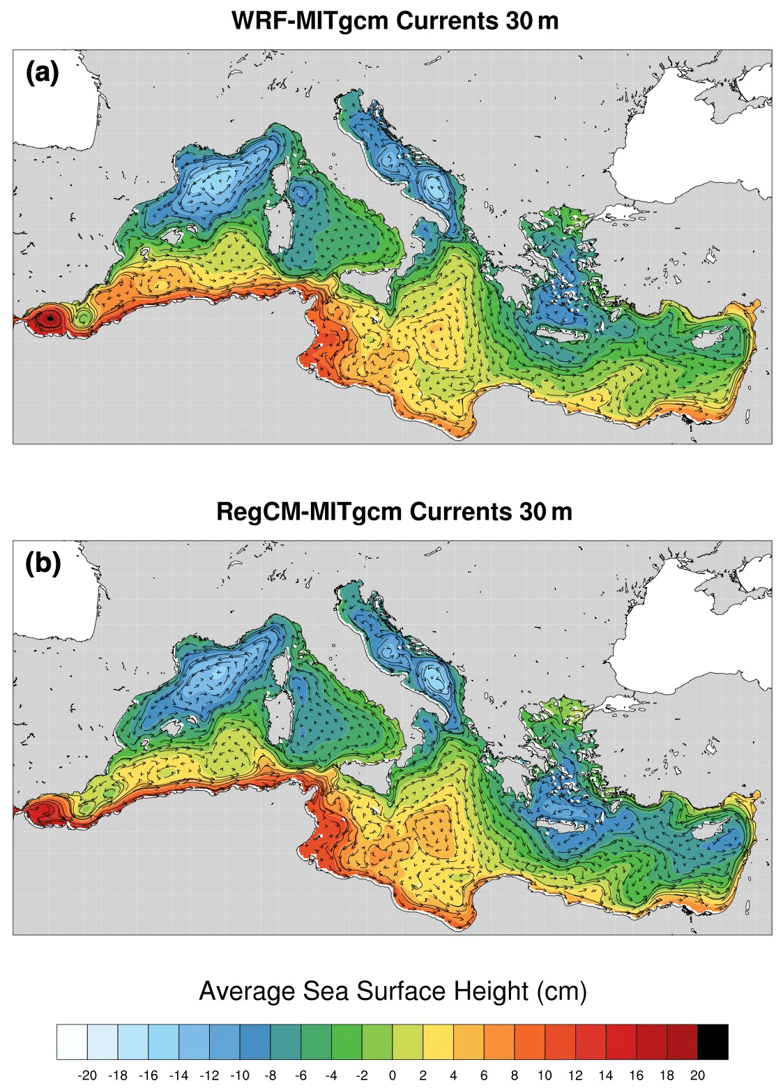
Figure 14 Mean annual sea surface elevation along with sub-surface (30 m) circulation as simulated by the two configurations of the coupled atmosphere–ocean model; data are averaged over the temporal period 1982–2013.

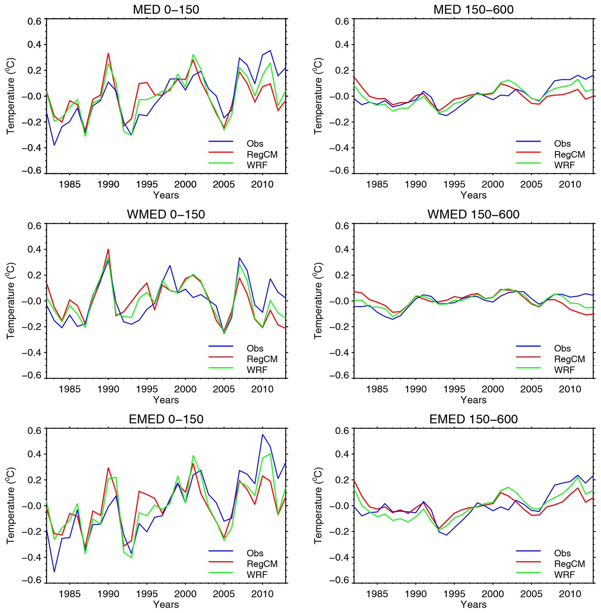
Figure 15 Annual mean temperature anomalies (^∘C) for upper (0–150 m) and intermediate (150–600 m) layers of the Mediterranean Sea, western and eastern basins, over the period 1982–2013.

The Atlantic Water (AW) circulation is in good agreement with those described by Millot and Taupier-Letage (2005) and Pinardi et al. (2015), the first being mainly based on both in situ and remotely sensed datasets, the latter resulting from a reanalysis performed with a model having a horizontal resolution of $\mathrm{1}/\mathrm{16}$^∘ × $\mathrm{1}/\mathrm{16}$^∘ . In particular, Atlantic surface waters enter at Gibraltar, are trapped into gyres in the Alboran Sea and then exit, dividing into two branches: one sticking to the North African coast, forming the Algerian current, and the other in the direction of the Balearic Islands. This latter branch detaches from the coast and flows south of Ibiza Island generating an intense jet flowing eastward. This current receives the contribution of the southern edge of the Lion cyclonic gyre after the Balearic Sea and generates the Southern Sardinian Current flowing along the west coast of Sardinia and merging with the Algerian current. The Southern Sardinian Current branches into three parts (Béranger et al., 2004; Pinardi et al., 2006): the southernmost branch produces the Sicily Strait Tunisian current, the central one forms the Atlantic Ionian Stream (Robinson et al., 1999; Onken et al., 2003; Lermusiaux and Robinson, 2001) and the northernmost one enters the Tyrrhenian Sea giving rise to the South-Western Tyrrhenian Gyre. Finally, the Atlantic waters penetrate into the eastern basin through the Sicily Strait. Noticeably, all these structures are very well defined in both the configurations of the regional Earth system model (Fig. 14). The two model's versions show the wide cyclonic gyre in the Gulf of Lion, which includes the Liguro-Provençal current, which is one of the main features of the western Mediterranean circulation.

The mean circulation in the eastern basin is characterized by several features common to both simulations. It is possible to appreciate how the surface water penetrates into the Adriatic Sea with a cyclonic circulation, and it is possible to note the presence of a counterclockwise circulation in the Aegean Sea in both simulations.

Moreover, the simulations reproduce quite clearly the places where deep-water formation takes place: the three cyclonic gyres located in the Gulf of Lion, the southern Adriatic Sea and in the Levantine Sea. These cyclonic gyres concur with negative SSH values, which highlight the sinking of surface waters.

4.2.3 Heat and salt contents

Mean annual temperature and salinity averaged over the entire Mediterranean Basin and the western and eastern sub-basins are shown in Table 3; here we present estimates from the MEDHYMAP data, while for the two simulations we show the anomalies with respect to the reference data. The average content of heat and salt has been computed over different vertical layers: the entire column, the surface layer (0–150 m) corresponding approximately to the Atlantic Water, the intermediate layer (150–600 m) representing mainly the Levantine Intermediate Water, and the deep layer (600–3500 m) containing the Eastern and Western Mediterranean Deep waters.

Table 3 Averaged temperature (^∘C) and salinity (psu) at different depths for the MEDHYMAP dataset and anomalies computed between the reference MEDHYMAP data and results from the coupled models. Values are averaged over the entire Mediterranean Sea and over the western and eastern basins (WMED and EMED, respectively) for the temporal period 1982–2013.

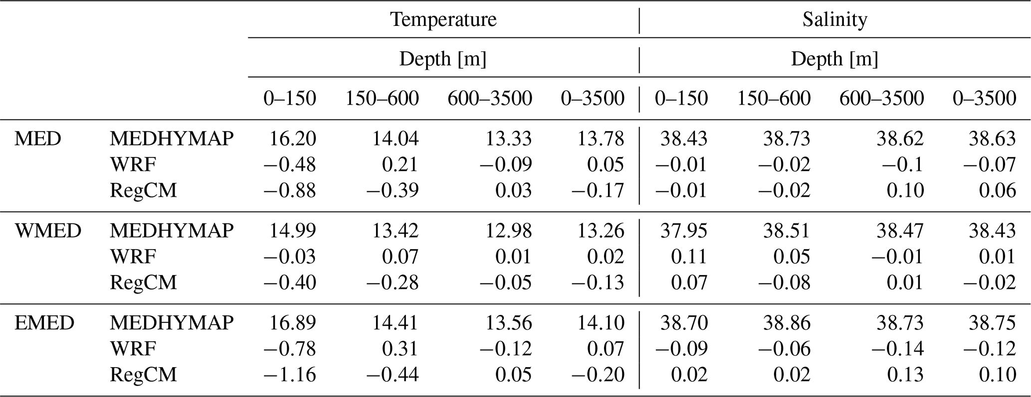
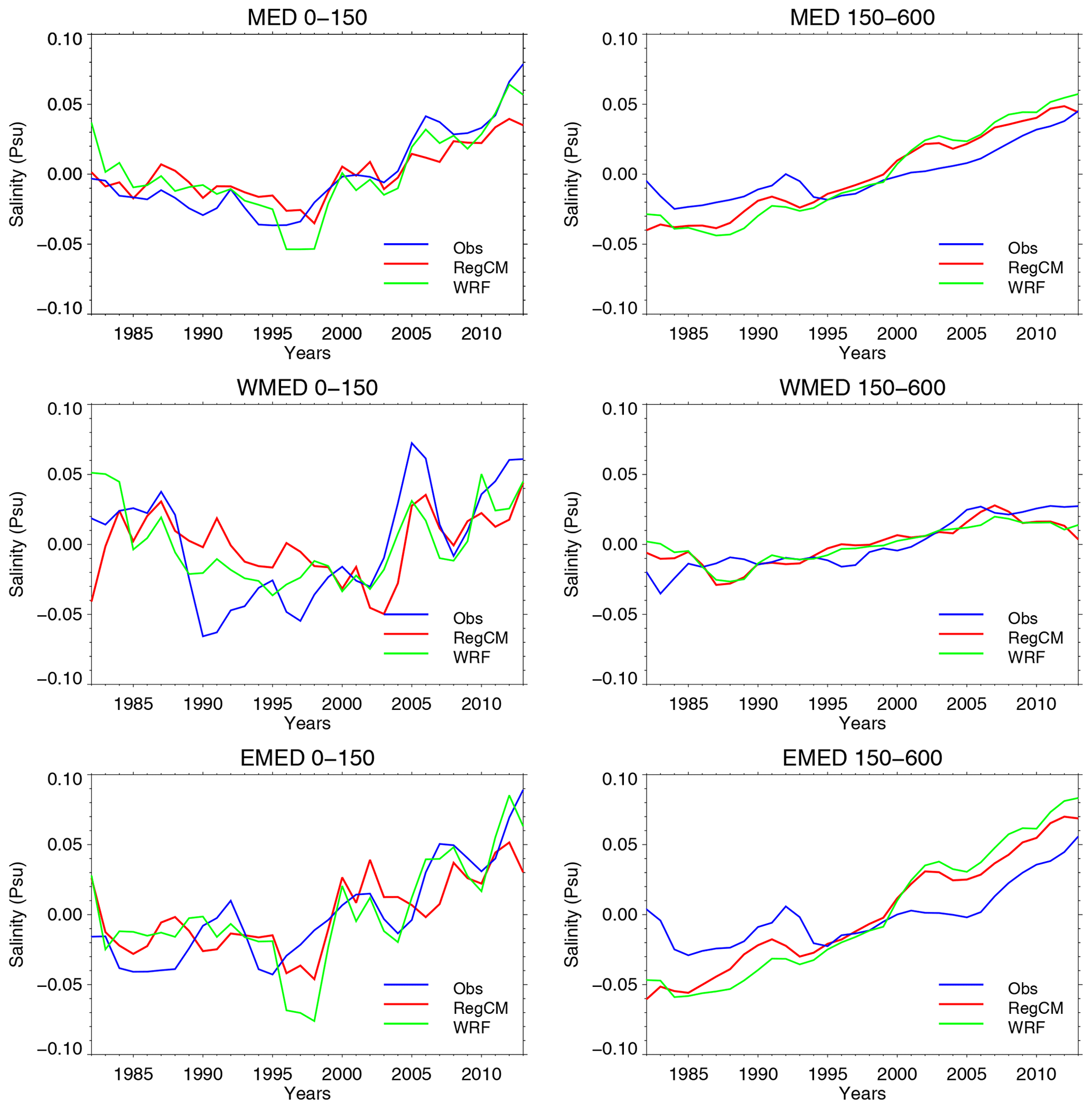
Figure 16 Annual mean salinity anomalies (psu) for upper (0–150 m) and intermediate (150–600 m) layers of the Mediterranean Sea, western and eastern basins over the period 1982–2013.

Figure 17 Time evolution of the maximum MLD computed over the Levantine Basin, Gulf of Lion area and Adriatic Sea for WRF–MITgcm (green) and RegCM–MITgcm (red) simulations.

The average temperature of the whole water column, for each sub-basin, is in good agreement with observations in both coupled runs, being the difference between modeled values and observations not exceeding 0.2 ^∘C. Major discrepancies are concentrated in the upper layer of the eastern basin, where both models are colder than observations. In particular, WRF–MITgcm shows a cold bias of 0.78 ^∘C, while RegCM–MITgcm has a bias exceeding 1 ^∘C. Such discrepancy reduces within the intermediate layer and deep layer in the case of WRF–MITgcm, while MITgcm forced by RegCM shows a slight overestimation in the deep layer, which mostly compensates for the error in the uppermost layer. In the western basin the two models remain much closer to the observations, with RegCM–MITgcm showing a systematic cold bias and WRF–MITgcm is closer to observations. Notwithstanding some biases, we point out that the mean values of the temperature within the different layers are compatible with those obtained in analogous simulations and are within the ensemble spread computed from the series of Med-CORDEX simulations analyzed by Llasses et al. (2018).

Figure 15 shows the time series of mean annual temperature anomalies computed over the 1982–2013 period for the surface and intermediate layers in the whole basin and in the western and eastern sub-basins. Generally, the interannual variability of the whole basin is captured well by the two simulations in both the surface layer and in the intermediate level with the two configurations showing similar variability and performances. However, the observations show a slight increasing trend, mainly in the eastern basin, that the simulations do not capture. In any case, both simulations capture the surface positive anomaly in 1990 in the western basin well, as well as the sequence of negative anomalies in the eastern basin (1983, 1987, and 1993). In the intermediate layer, the sudden drop of temperature during 1993 is the signature of the Eastern Mediterranean Transient (EMT) phenomenon (discussed in Sect. 4.2.4).

The mean annual salinity averaged over the whole column (Table 3) is slightly underestimated by WRF–MITgcm (−0.07 psu) and overestimated by RegCM–MITgcm (0.06 psu). In the eastern basin the maximum of salinity is correctly found in the intermediate layer (150–600 m), corresponding to the Levantine Intermediate Water (LIW), although the RegCM–MITgcm simulation shows too slight a decrease in the salinity from the intermediate to the deep layer. Such behavior is consistent with the higher values reached by the mixed layer depth (MLD) in the same area with respect to the MLD of the WRF–MITgcm simulation (discussed in Sect. 4.2.4).

Similarly, in the western basin saltier intermediate water is clearly identified in the WRF run with respect to RegCM, due to the combined effect of the advection of a saltier LIW and a less intense deep convection, and in the western basin is mostly concentrated in the Gulf of Lion area. The comparison of the MLD in the Gulf of Lion area (see Sect. 4.2.4) supports this hypothesis.

Figure 16 shows the time series of mean annual salinity anomalies computed over the 1982–2013 period for the surface and intermediate layers in the whole basin and in the western and eastern sub-basins. While the entire basin variability is generally reproduced well, the behavior of models in the two sub-basins deserves some comment. In particular, in the western basin the MITgcm, in its two configurations, the simulation fails in reproducing the drop in salinity of the uppermost layer during the years 1990–1995. This is probably due to a too low freshwater flux simulated by the atmospheric components in those years, confirmed by high values of the MLD. On the other hand, in the eastern basin the WRF–MITgcm shows a large freshwater anomaly in the 0–150 m layer during the years 1995–1997 that is not detectable in the reference data. However, it should be noted that the same anomaly has also been observed in the SSS time series and is caused by exceptional precipitation and river runoff as already reported by Sevault et al. (2014). In any case, such a drop seems to affect mainly SSS and the surface layer, while it is scarcely transferred below 200 m. In the intermediate layer both simulations show a steady increase in the salinity anomaly. RegCM–MITgcm has an almost linear increase throughout the entire simulation period, due to the excess of surface salinity and anomalous deep convection in the Levantine Sea, while WRF–MITgcm is quite stable during the first half of the simulations and then shows a steep linear increase from 2000 onward.

4.2.4 Deep-water formation

The formation of intermediate and deep waters due to the sinking of dense water is one of the fundamental processes taking place in the Mediterranean Sea, in both the eastern and western sub-basins. Typical regions interested in this process are the Gulf of Lion, the South Adriatic Sea, the Cretan Sea and the Rhodes Gyre. Such a process, mainly driven by the strong air–sea interactions, takes place during the winter season and is more effective during February. The most active regions for deep-water formation are the Gulf of Lion and the Adriatic Sea, while intermediate waters are usually formed in the Levantine Sea.

The MLD is related to thermodynamic properties of seawater and is a pivotal variable helping in the identification of deep-water formation events. High MLD values are related to strong air–sea processes taking place at the surface or to preexisting stratification of the whole water column.

Figure 17 compares the simulated monthly maximum MLD computed over the most important convective areas, i.e., the Levantine Sea, the Gulf of Lion and the Adriatic Sea. In general, RegCM–MITgcm shows a more intense convection activity with respect to WRF–MITgcm, often reaching the deepest levels in all the analyzed regions. Looking at the Levantine region (Fig. 17a), during almost the entire simulation, the MLD simulated by RegCM–MITgcm exceeds 1000 m depth, while in the case of WRF–MITgcm there are a few events where the MLD is confined to the intermediate level (400–500 m). The strong events of 1983, 1987 and 1989 are clearly detectable in both simulations and correspond to intense atmospheric fluxes, which have favored the preconditioning of the eastern basin leading to the well-known phenomenon of the EMT. In the Gulf of Lion, both simulations show an intense convection activity that often reaches the bottom of the column in at least one of the two models, with the exception of the years 1989, 1990 and 2007. The other site of deep-water formation is the South Adriatic zone, where the two models are in remarkably good agreement one with each other.

In addition to the temporal evolution of MLD, in Fig. 18 we compare the mean spatial pattern of the MLD with ARGO data (Holte et al., 2017). Results suggest that the downwelling regions of both simulations are much more extended compared to ARGO data, and in RegCM–MITgcm the convective area is slightly wider than in the WRF–MITgcm simulation.

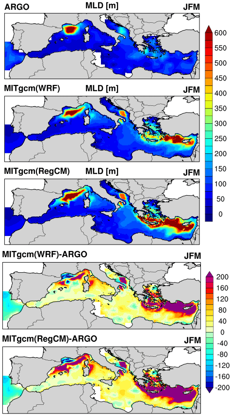
Figure 18 Winter (JFM) spatial pattern (upper three rows) and bias (lower two rows) of mixed layer depth (MLD [m]) as simulated by the coupled model using the two atmospheric components as forcing (i.e., WRF and RegCM) and the ARGO dataset between 1982 and 2013. Note that ARGO data are interpolated into the ocean model grid for comparison purposes.

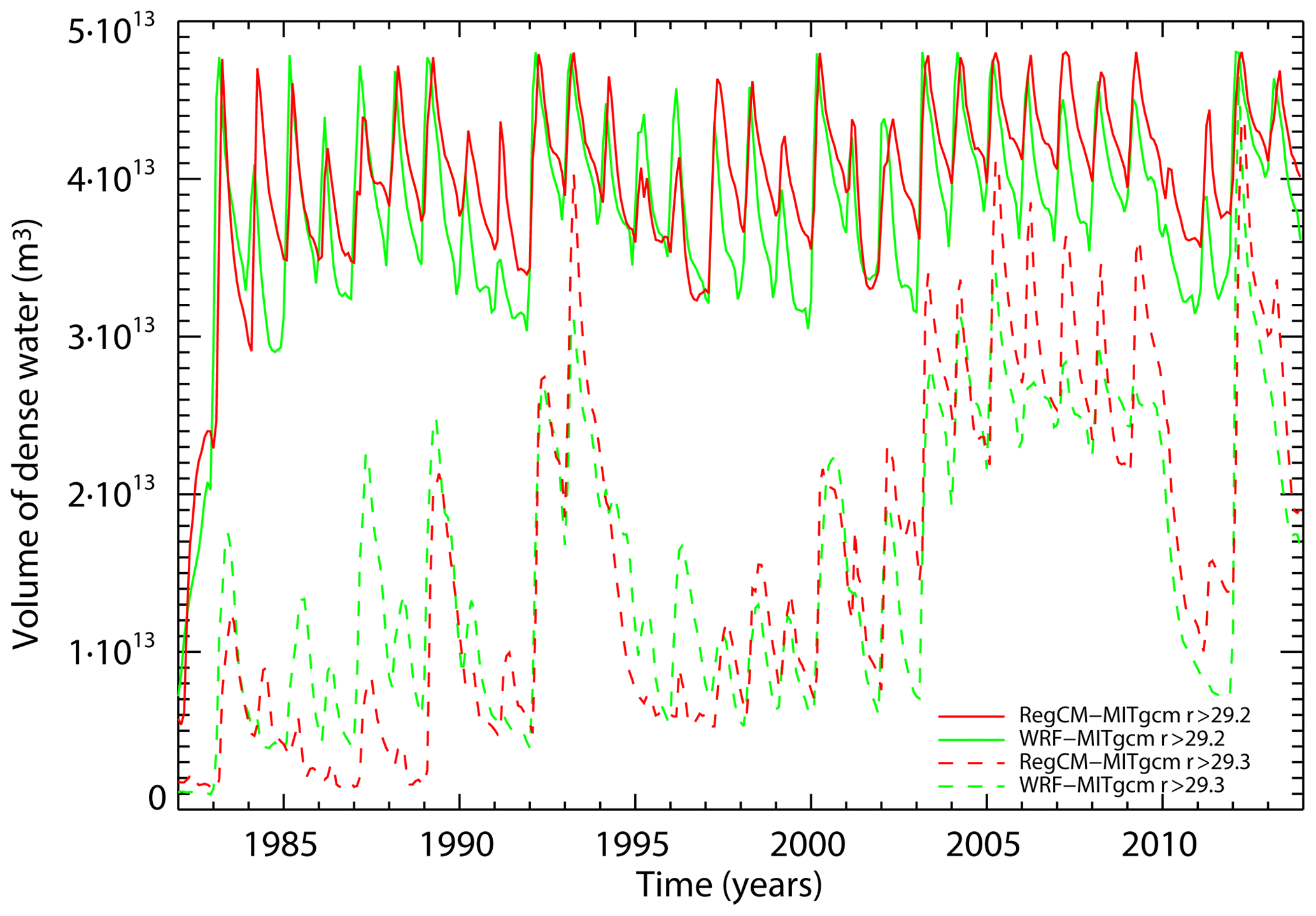
Figure 19 Monthly volume of water denser than 29.2 kg/m³ (solid line) and denser than 29.3 kg/m³ (dashed line) produced in the Cretan Sea for the two configurations of the ENEA-REG system.

The steady-state picture of the Mediterranean thermohaline circulation, in which the Eastern Mediterranean Deep Water (EMDW) is only of Adriatic origin, has been called into question by the discovery of the EMT. As described by many authors, there is observational evidence that during the 1990s the main source of EMDW migrated to the Aegean Sea (Lascaratos et al., 1993; Malanotte-Rizzoli et al., 1999; Wu et al., 2000; Roether et al., 2007; Beuvier et al., 2010). The common understanding is that the EMT has been the effect of many concurrent causes that make this process difficult to simulate: the large heat loss from the surface in the Levantine, the shifting from cyclonic to anticyclonic circulation in the Ionian that prevents the entering of freshwater into the Levantine Basin, and the lower than usual freshwater flux from the Black Sea. Waters formed in the Aegean are warmer and saltier than that of the eastern Mediterranean at the same levels, and they are found at intermediate levels between LIW and EMDW of Adriatic origin. During the EMT period, instead, bottom levels were filled with newly formed waters of Aegean origin, while the less dense Adriatic waters were uplifted (Roether et al., 2007). All the studies agree on a massive dense-water formation in the Aegean Sea during the period 1987–1994 (e.g., Theocharis et al., 2002); as described by Theocharis et al. (1999), during the period 1986–1987, the Cretan Sea was characterized by a weak stratification. In the following years, water with densities higher than 29.2 was found at progressively higher layers in the Cretan Sea, with a significant formation rate in particular during 1989, due to an intrusion of deep waters from the central Aegean through the Mykonos–Ikaria strait (Vervatis et al., 2013). Starting from 1989 dense water outflowed from the Cretan Arcs and was found in the eastern Mediterranean Sea at levels between 700 and 1600 m. Then, dense water formation in the Cretan Sea increased during 1991 and 1992, the new water reached the upper layer of the Cretan Basin, and the entire basin was filled with young water with a density of up to 29.3.

This phenomenon is remarkably reproduced well by the two configurations of the model, both considering the timing of events and the density and volumes of newly formed waters, as shown in Fig. 19. Here the volumes occupied by water with a density higher than 29.2 and 29.3 kg/m³ in the Cretan Sea are shown; it can be seen that the period between 1983 and 1993 is characterized by an increase in the volume with the three most significant peaks in 1984, 1989, and 1993 (the highest peak), in both the simulations.

5 Summary and conclusions

We presented a newly designed regional Earth system model to study the climate variability over the Euro-Mediterranean region. The performances of individual model components were evaluated comparing results from the simulations with a wide range of observation-based datasets.

Unlike other existing regional coupled atmosphere–ocean models, our system is made up of two interchangeable atmospheric components (i.e., RegCM and WRF), offering the capability to select the regional atmospheric model to be used depending on the region of interest and the model's performances over the selected region. We performed a hindcast simulation for each atmospheric configuration over the period 1980–2013 using ERA-Interim reanalysis as lateral boundary conditions.

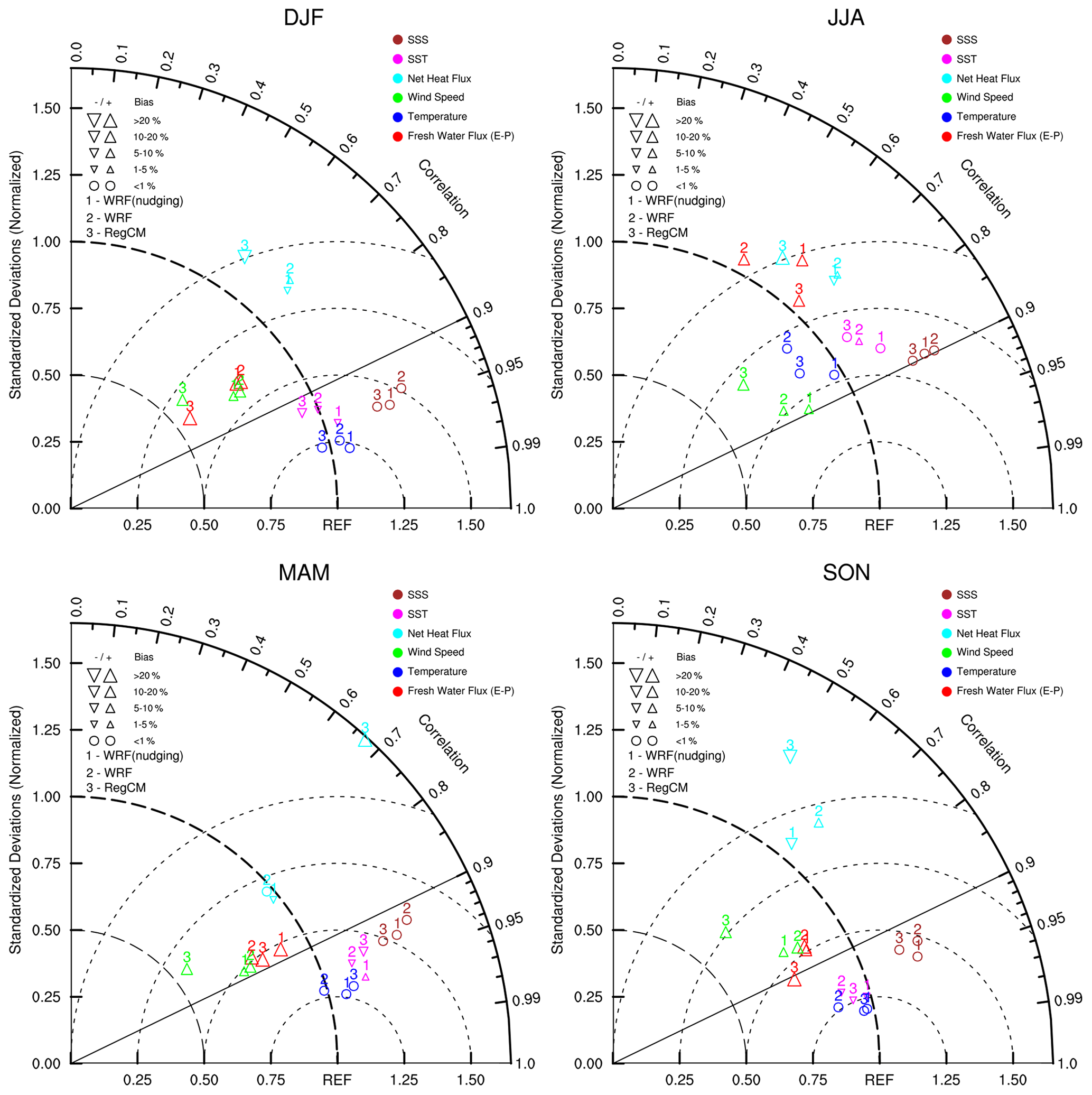
Figure 20 Taylor diagram showing the meteorological variables simulated by the atmospheric components of the regional Earth system model and exchanged with the ocean component as well as surface temperature and salinity simulated by the MITgcm. Solid line indicates the centered correlation patterns, while gray dashed lines represent the root mean standard error. Finally size and shape of markers are used to identify the bias.​​​​​​​

Overall, results indicate that the two atmospheric components of the regional Earth system model (i.e., WRF and RegCM) correctly reproduce both large-scale and local features of the Euro-Mediterranean climate, although we found some remarkable biases for some variables. While WRF shows a significant cold bias during winter over the northeastern area of the domain and a large warm bias during summer, RegCM overestimates the wind speed over the Mediterranean Sea.

The ocean component correctly reproduces the analyzed surface ocean properties (along with their interannual variability) and the observed circulation in both the coupled model configurations. In any case, because of the wind speed overestimation by RegCM, we found a cold bias in the SST during the winter months.

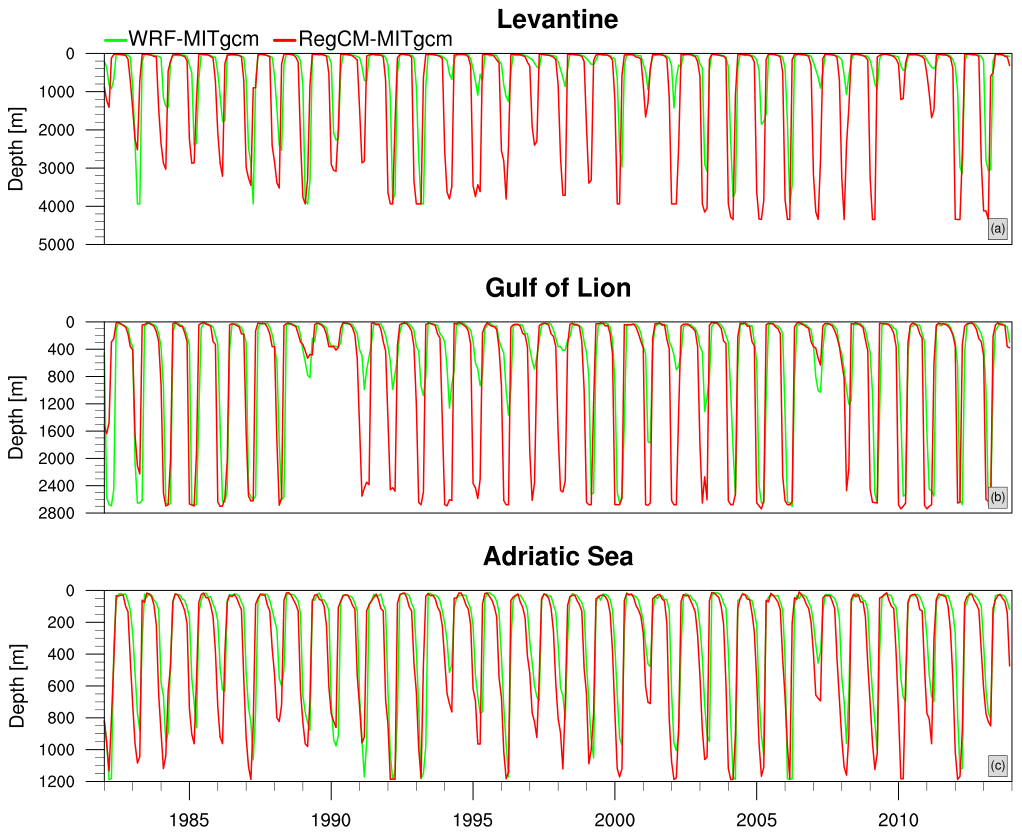
Figure 21 Time evolution of the maximum MLD computed over the Levantine Basin, Gulf of Lion area and Adriatic Sea for WRF–MITgcm with nudging (green) and RegCM–MITgcm (red) simulations.

A possible approach aimed to reduce the biases is the adoption of nudging techniques, recently introduced into some RCMs (Liu et al., 2012). This method allows the passing of the driving model information not only onto the lateral boundaries but also into the interior of the regional model domain (Waldron et al., 1996; Heikkilä et al., 2011); this is achieved by relaxing the model state towards the large-scale driving fields by adding a non-physical term to the model equation (Omrani et al., 2015). Clearly, the nudging allows a stronger control by the driving forcing and thus a greater consistency between the regional model and large-scale climate coming from the driving model. However, nowadays, there is still some controversy about the use of indiscriminate nudging in regional climate models (e.g., Omrani et al., 2015). Some studies agree that nudging does not allow the regional model to deviate much from the driving fields limiting the internal physics of the regional climate model (e.g., Sevault et al., 2014; Giorgi, 2019). Considering the atmosphere–ocean coupling, Sevault et al. (2014) conclude that the use of spectral nudging strongly constrains the synoptic chronology of the atmospheric flow and thus the chronology of the air–sea fluxes and the ocean response; they also found that this facilitates day-to-day and interannual evaluation with respect to observations, but nudging also limits the internal variability of the atmospheric component of the coupled model. Conversely, in a different study on extreme events in the Mediterranean Sea performed with a coupled atmosphere–ocean model, Lebeaupin-Brossier et al. (2015) found that nudging does not inhibit small-scale processes; thus, potential air–sea feedbacks are correctly simulated. This result is consistent with Omrani et al. (2015), who suggested that the spectral nudging technique does not affect the small-scale fields since only the large scales are relaxed.

Not all RCMs offer the possibility to use nudging; for example, WRF can be used with spectral or grid nudging (Liu et al., 2012), while RegCM cannot. To assess the impact of nudging on the performance of a coupled model, we performed an additional coupled simulation with WRF–MITgcm using the spectral nudging; the overall performances of the regional model in its three versions are summarized for the relevant variables over the Mediterranean Sea with a Taylor diagram (Fig. 20). Results indicate that WRF with nudging performs better than the simulation without nudging in most analyzed meteorological variables. However, the most interesting result is that the ocean physical processes are much better represented and agree with observation-based data when nudging is used in the atmospheric component. In particular, intermediate and deep-water formation are much better represented. Figure 21 shows the intercomparison between the WRF–MITgcm with nudging and the RegCM–MITgcm simulation as representative of the simulations performed without nudging. While in the Levantine Sea, the MLD simulated by RegCM–MITgcm exceeds 1000 m depth, and WRF–MITgcm MLD is more variable in time. The latter reaches the entire water depth during a few events, which are well known and documented with in situ observations (Lascaratos et al., 1999; Malanotte-Rizzoli et al., 1999; Roether et al., 2007). Therefore, we can conclude, as expected, that the LIW formation is better reproduced when the nudging is applied. Several MLD observation-based estimates are available in the Gulf of Lion for the period covered by our simulations (e.g., Mertens and Schott, 1998; Schroeder et al., 2008; Somot et al., 2018a). Compared to these estimates, we observe that the WRF–MITgcm simulation closely follows the timing of deep-water formation in the western Mediterranean, in particular the deep convection events of 1987 and 2005, with the exception of 1991 and 1992, identified by Somot et al. (2018a) as years of intense mixing, while RegCM–MITgcm systematically presents a deeper MLD (Fig. 21b). The deep convection in the Adriatic does not change significantly due to the nudging, always involving the entire column depth.

This analysis reveals that spectral nudging helps to keep the large-scale circulation of the regional model closer to the driving model; however, we remark that nudging does not avoid the model to develop the small-scale processes such as those relevant in the Gulf of Lion. This is a crucial point for the entire thermohaline circulation of the Mediterranean Sea. The striking correspondence with observed data in this region depends on the good representation of the local wind, the mistral, and the correct stratification of the whole column water, with the Levantine Intermediate Water coming from the eastern basin playing a crucial preconditioning role. Notwithstanding the added value of nudging proved by the better performance of the WRF–MITgcm configuration, nudging has also to be used with caution: strong inconsistencies between the regional model and large-scale driving fields may lead to unrealistic compensations within the model, for example, anomalous heat fluxes compensating for temperature biases (Brune and Baehr, 2020).

This study presented two different configurations of the same regional Earth system model, differing for the atmospheric component and using the same version of the ocean model. Our main result is that the two configurations are comparable and consistent with the previous results available in the literature. Thus they can be used to realize future climate scenario simulations, contributing to the realization of regional ensembles. On the other hand, we can perform hindcast simulations very close to observations, once we have switched to an atmospheric model that offers the opportunity to use the spectral nudging technique.