FALL3D-8.0: a computational model for atmospheric transport and deposition of particles, aerosols and radionuclides – Part 2: Model validation

This paper presents model validation results for the latest version release of the FALL3D atmospheric transport model. The code has been redesigned from scratch to incorporate different categories of species and to overcome legacy issues that precluded its preparation towards extreme-scale computing. The model validation is based on the new FALL3D-8.0 test suite, which comprises a set of four real case studies that encapsulate the major features of the model; namely, the simulation of long-range fine volcanic ash dispersal, volcanic SO₂ dispersal, tephra fallout deposits and the dispersal and deposition of radionuclides. The first two test suite cases (i.e. the June 2011 Puyehue-Cordón Caulle ash cloud and the June 2019 Raikoke SO₂ cloud) are validated against geostationary satellite retrievals and demonstrate the new FALL3D data insertion scheme. The metrics used to validate the volcanic ash and SO₂ simulations are the structure, amplitude and location (SAL) metric and the figure of merit in space (FMS). The other two test suite cases (i.e. the February 2013 Mt. Etna ash cloud and associated tephra fallout deposit, and the dispersal of radionuclides resulting from the 1986 Chernobyl nuclear accident) are validated with scattered ground-based observations of deposit load and local particle grain size distributions and with measurements from the Radioactivity Environmental Monitoring database. For validation of tephra deposit loads and radionuclides, we use two variants of the normalised root-mean-square error metric. We find that FALL3D-8.0 simulations initialised with data insertion consistently improve agreement with satellite retrievals at all lead times up to 48 h for both volcanic ash and SO₂ simulations. In general, SAL scores lower than 1.5 and FMS scores greater than 0.40 indicate acceptable agreement with satellite retrievals of volcanic ash and SO₂. In addition, we show very good agreement, across several orders of magnitude, between the model and observations for the 2013 Mt. Etna and 1986 Chernobyl case studies. Our results, along with the validation datasets provided in the publicly available test suite, form the basis for future improvements to FALL3D (version 8 or later) and also allow for model intercomparison studies.

1 Introduction

FALL3D-8.0 is the latest major version release of FALL3D (Costa et al., 2006; Folch et al., 2009), an open-source code with a 15-year+ track record and a growing number of users in the volcanological and atmospheric science communities. A companion paper (Folch et al., 2020) details the physics and the novel numerical implementation of the code, which has been redesigned and rewritten from scratch in the framework of the EU Centre of Excellence for Exascale in Solid Earth (ChEESE). From the point of view of model physics, a relevant improvement in the new version (v8.x) has been the generalisation of the code to deal with atmospheric species other than tephra including other types of particles (e.g. mineral dust), gases and radionuclides (see Table 3 in Folch et al., 2020, for details). These different categories and subcategories of species can be simulated using independent sets of bins that allow for dedicated parameterisations for physics, emissions (source terms) and interactions among bins (e.g. aggregation, chemical reactions, radioactive decay). In FALL3D, “tephra” species are subdivided into four subcategories, depending on particle diameter, d (Folch et al., 2020): (i) fine ash (d≤64 µm), (ii) coarse ash (64 µm $<d\le \mathrm{2}$ mm), (iii) lapilli (2 mm $<d\le \mathrm{64}$ mm) and (iv) bomb (d>64 mm). In terms of model performance, the new model version contains a much more accurate and less diffusive solver, as well as a better memory management and parallelisation strategy that notably outperforms the scalability and the computing times of the precedent code version (v7.x) (Folch et al., 2020). This paper complements the Folch et al. (2020) companion paper by presenting a detailed set of validation examples, all included in the new test suite of the code. This paper also contains some novel aspects regarding geostationary satellite detection and retrieval of volcanic ash (Appendix A) and SO₂ (Appendix B), as well as the FALL3D-8.0 data insertion methodology. To furnish the initial model condition required for data insertion, the satellite retrievals are collocated with lidar measurements of cloud-top height and thickness from the CALIPSO (Cloud-Aerosol Lidar and Infrared Pathfinder Satellite Observation) platform (Winker et al., 2009). The data insertion scheme is a preliminary step towards model data assimilation using ensembles, a novel functionality currently under development.

The paper is organised as follows. Section 2 provides an overview of the model test suite, detailing the file structure and contents for each of the four case studies considered for validating and testing FALL3D-8.0. Section 3 provides a description of each of the events making up the test suite, which include simulations of the June 2011 Puyehue-Cordón Caulle ash cloud, the June 2019 Raikoke SO₂ cloud, the February 2013 Mt. Etna ash cloud and associated tephra fallout deposit, and the dispersal of radionuclides resulting from the 1986 Chernobyl nuclear accident. The datasets used for validation and the FALL3D model configurations used in each case are also contained in Sect. 3. Section 4 describes the validation metrics, which include the structure, amplitude and location (SAL) metric (Wernli et al., 2008) and the figure of merit in space (FMS; Galmarini et al., 2010; Wilkins et al., 2016) to quantitatively compare model results with satellite retrievals, along with the root-mean-square error (RMSE) for validation of the ground deposit simulations of tephra and radionuclides. Section 5 presents a detailed discussion of the validation results for the four test suite cases. Finally, Sect. 6 presents the conclusions of the paper and outlines the next steps in terms of model development and applications.

2 The FALL3D-8.0 test suite

FALL3D-8.0 includes both a benchmark and a test suite. The benchmark suite consists of a series of non-public small-case tests used by model developers for model verification and code performance analysis. These benchmark cases are typically passed when substantial model updates in the master branch of the code are committed to the repository and, essentially, contain idealised 1-D or 2-D cases with known analytical solutions for verification purposes (see, e.g. Figs. 3, 4 and 5 in Folch et al., 2020). In contrast, the test suite includes larger-size, real-case simulations aimed at model validation. Model users can download the public test suite repository files to run the model and to check whether it has been properly installed and configured on their local machines. This paper presents the four cases from the FALL3D-8.0 test suite listed in Table 1; namely, Puyehue-2011 (simulation of the June 2011 Puyehue-Cordón Caulle ash cloud), Raikoke-2019 (simulation of the June 2019 Raikoke SO₂ cloud), Etna-2013 (simulation of the 23 February 2013 Mt. Etna ash cloud and related tephra fallout deposit) and Chernobyl-1986 (simulation of the dispersal and deposition of radionuclides resulting from the April 1986 Chernobyl nuclear accident). Note that the names of the validation cases are shown in bold throughout this paper. The FALL3D-8.0 test suite repository contains independent folders (one per validation case). All case folders have the same subfolder structure:

• InputFiles. This subfolder contains all the necessary input files to run the case. The only exception is meteorological data because these typically involve substantially large files (tens of gigabytes) that make the storage and the transfer to/from the GitLab public repository unpractical/unfeasible.

• Utils/Meteo. This subfolder contains all the necessary files to obtain meteorological data depending on the meteorological driver (for possible options, see Table 12 in Folch et al., 2020). For global datasets such as the ERA5 dataset (Copernicus Climate Change Service, 2017) used in the Puyehue-2011 case, Python and shell scripts are provided so that the user can download and merge meteorological data consistently with the SetDbs pre-process task (see Sect. 5 in Folch et al., 2020). For mesoscale datasets (e.g. the WRF-ARW dataset used in the Etna-2013 case), the subfolder includes the meteorological model “namelists” and scripts to download the global data driving the corresponding mesoscale model simulation.

• Utils/Validation. This subfolder contains all the necessary files to validate the FALL3D-8.0 model execution results, including a file with the expected validation metric results.

Table 1 Summary of model setups for the test suite validation cases shown in this paper.

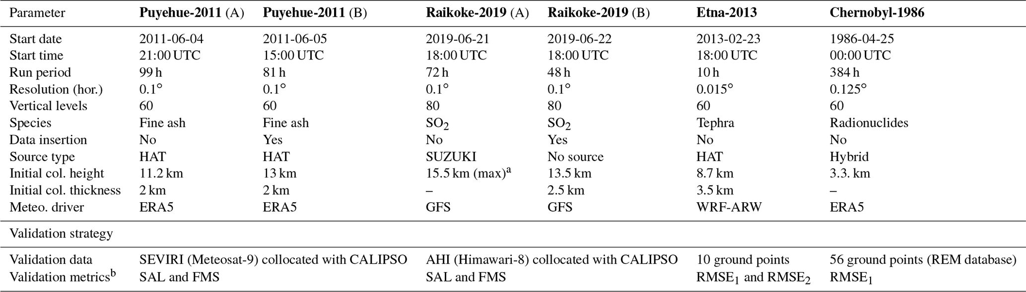
^a Variable column height between 3.5 and 15.5 km. ^b Validation metrics are defined in Sect. 4.

Table 2 Description of the files in the Puyehue-2011 test suite folder (see Sect. 3.1).

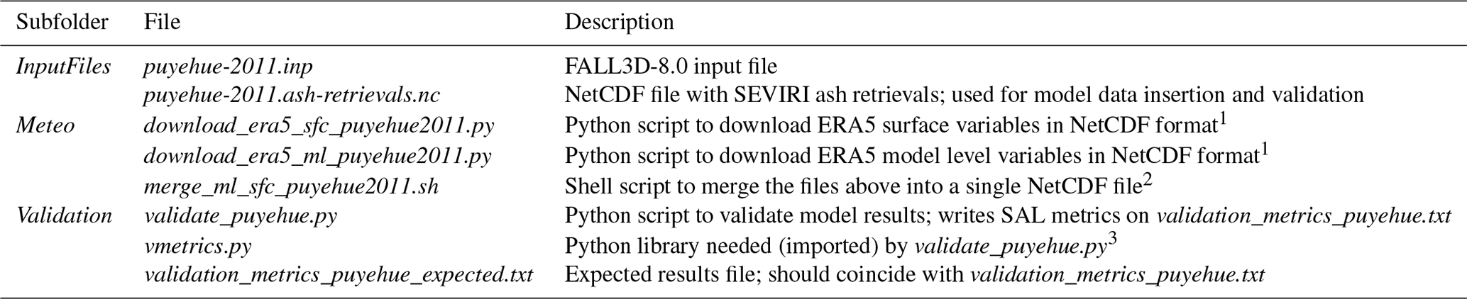
¹ Makes use of Climate Data Store (CDS) Application Programming Interface (API) of the Copernicus CDS. ² Makes use of Climate Data Operators (CDO). ³ Makes use of netCDF4, numpy, datetime, pandas and scipy Python libraries.

Table 3 Description of the files in the Etna-2013 test suite folder (see Sect. 3.3).

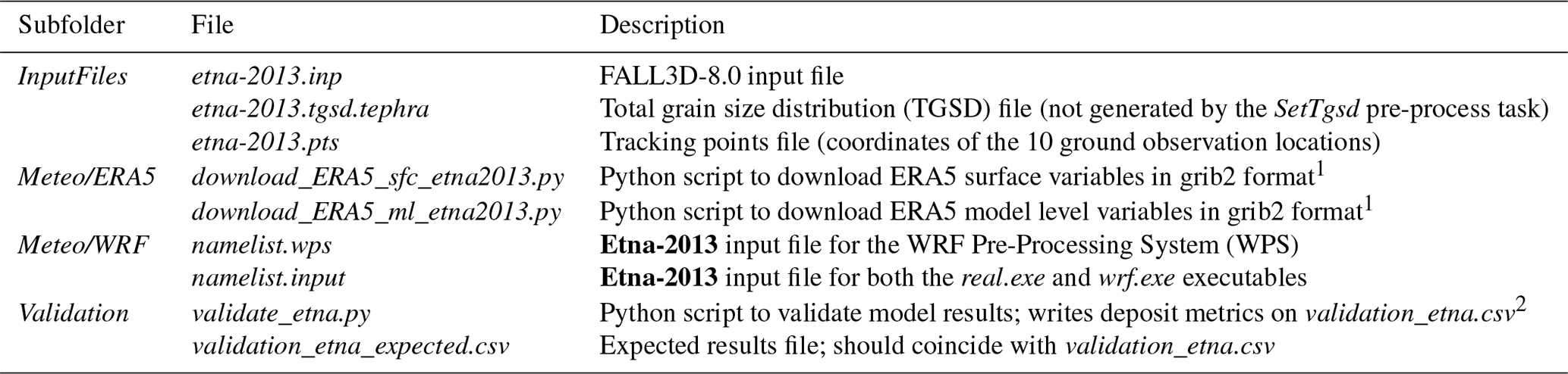
¹ Makes use of CDS API of the Copernicus Climate Data Store. ² Makes use of pandas, glob, os and sys Python libraries.

Tables 2 and 3 list the files in the test suite for the Puyehue-2011 (Sect. 3.1) and the Etna-2013 (Sect. 3.3) cases, respectively. The Raikoke-2019 (Sect. 3.2) and Chernobyl-1986 (Sect. 3.4) filenames look very similar to the Puyehue-2011 and Etna-2013 filenames and are not explicitly shown here. In all cases, the test suite contains the necessary information to reproduce all of the simulation and validation results shown in the present study.

3 Validation cases

3.1 Puyehue-2011

The Puyehue-Cordón Caulle volcanic complex (PCCVC), located in the southern volcanic zone of the central Andes, comprises a 20 km long, NW–SE-oriented fissure system (Cordón Caulle) and the Puyehue stratovolcano (Elissondo et al., 2016). On 4 June at around 14:45 LT (18:45 UTC), a new vent opened at 7 km NNW from the Puyehue volcano (Collini et al., 2013), initiating a remarkable example of a long-lasting plume with complex dynamics, strongly influenced by the interplay between eruptive style, atmospheric winds and deposit erosion (Bonadonna et al., 2015). The initial explosive phase of the eruption (4–14 June) was characterised by the development of eruption columns with heights oscillating between 6 and 14 km above sea level (a.s.l.), which correspond approximately to 4–12 km above the vent. Plume heights progressively decreased (4–6 km a.s.l.) between 15 and 30 June and low-intensity ash emission persisted for several months (Elissondo et al., 2016). Due to the predominant westerly winds, ash was transported towards Argentina and a wide area of the arid and semi-arid regions of northern Patagonia was severely affected by tephra dispersal and fallout. The PCCVC event stands as one of the most extraordinary examples of long-range fine ash transport observed by satellite and is the reason for selecting it as a validation case in the present study.

3.1.1 Validation dataset

In order to validate FALL3D-8.0 simulations of dispersal of fine ash and to test the new volcanic ash data insertion scheme, we use the retrieval method of Prata and Prata (2012) to derive fine ash mass loading estimates based on infrared (IR) measurements made by the SEVIRI (Spinning Enhanced Visible and Infrared Imager; Schmetz et al., 2002) instrument (aboard Meteosat-9) during the 2011 Puyehue-Cordón Caulle eruption in Chile. For IR wavelengths, SEVIRI samples the Earth's full disk every 15 min with a spatial resolution of 3 km × 3 km at the subsatellite point. After applying the Prata and Prata (2012) retrieval algorithm to SEVIRI at its native resolution, we resample the data onto a regular latitude–longitude grid of 0.1^∘ × 0.1^∘ (using nearest neighbour resampling), consistent with the FALL3D output grid. The satellite observations we consider for the Puyehue case study cover the time period from 00:00 UTC on 5 June 2011 to 00:00 UTC on 10 June 2011 and have a temporal resolution of 1 h (121 time steps). Details of the retrieval algorithm implementation and specific ash detection thresholds adopted for the Puyehue case study are provided in Appendix A.

3.1.2 Model setup

To simulate long-range, fine volcanic ash (d≤64 µm) transport from the Puyehue-Cordón Caulle eruption, we carried out FALL3D runs in two configurations. The first configuration (listed as Puyehue-2011 (A) in Table 1) was initialised at 21:00 UTC on 4 June 2011 for a duration of 99 h with a continuous emission source term. The source term was defined as a uniform distribution (HAT option) with a column height of 11.2 km a.s.l. (9 km above vent level) and 2 km column thickness. The second configuration (listed as Puyehue-2011 (B) in Table 1) demonstrates the new data insertion scheme which was recently introduced in FALL3D-8.0 as described in Folch et al. (2020). The data insertion run was initialised at 15:00 UTC on 5 June 2011, which coincides with a CALIPSO overpass that intersected the nascent ash plume (see Fig. A4b). To constrain the vertical distribution of ash in FALL3D, we collocated the CALIOP (Cloud-Aerosol Lidar with Orthogonal Polarization) total attenuated backscatter profiles with ash-affected SEVIRI pixels. Note that the vertical distribution is only required for the data insertion time. Based on these coincident observations we set the cloud-top height and thickness of the data-inserted ash cloud to 13 km a.s.l. and 2 km, respectively. In addition, to account for ash erupted after the data insertion time, we initialised the same source term specified in the Puyehue-2011 (A) configuration (i.e. continuous, uniform source emission up to 11.2 km a.s.l.) at the data insertion time (15:00 UTC on 5 June 2011). For both model configurations, the meteorological dataset used was ERA5 reanalysis (Copernicus Climate Change Service, 2017), which has a horizontal spatial resolution of 0.25^∘ and 137 model levels. The output domain size in both cases was set to 15–75^∘ S and 20–55^∘ W (0.1^∘ latitude–longitude grid resolution). Fine ash species were considered for both model configurations to simulate airborne PM₁₀ mass loadings. Further details of both model configurations are summarised in Table 1.

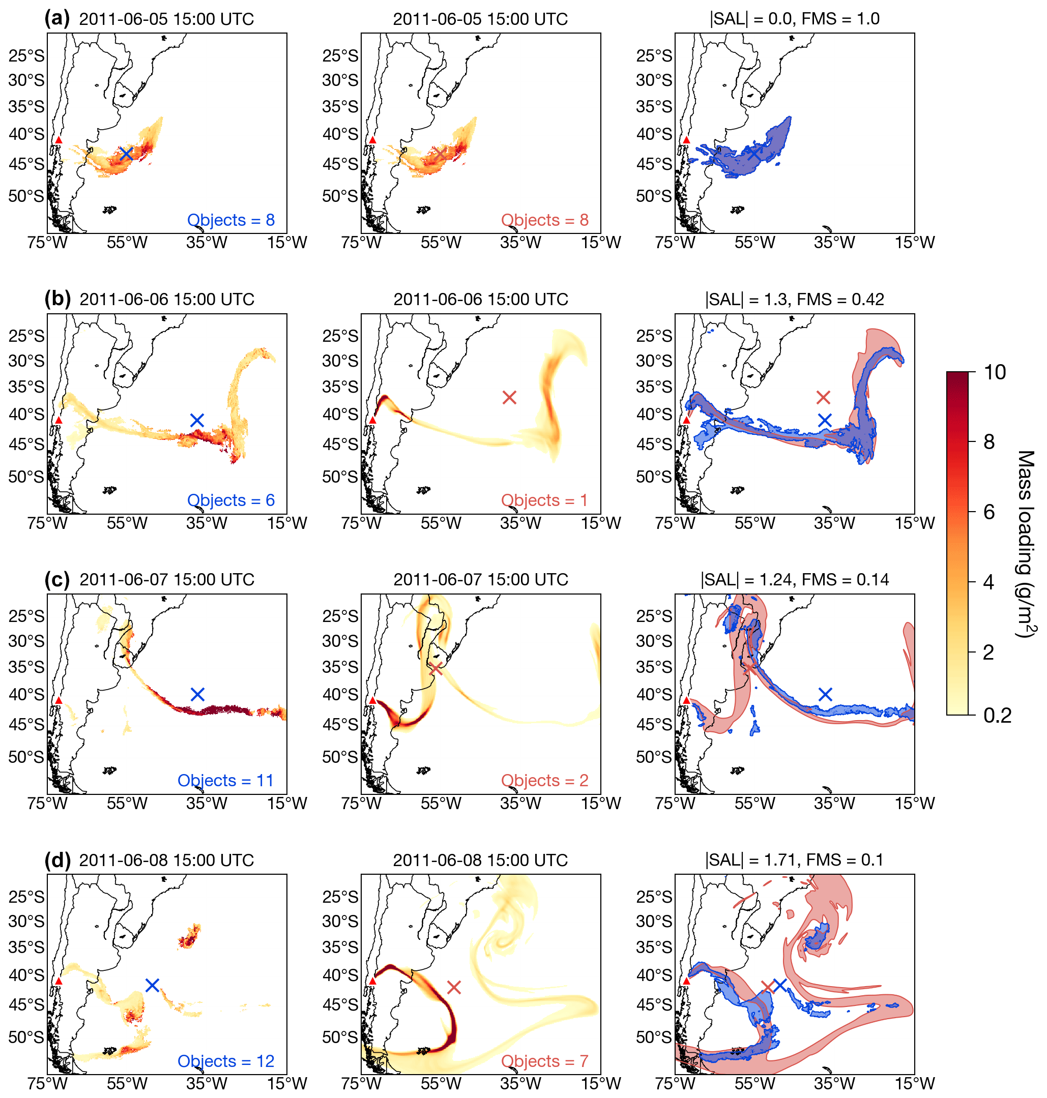
Figure 1 Puyehue-2011 test validation results for fine ash mass loading using SEVIRI retrievals on (a) 5 June 2011 at 15:00 UTC (data insertion time), (b) 6 June 2011 at 15:00 UTC, (c) 7 June 2011 at 15:00 UTC and (d) 8 June 2011 at 15:00 UTC. Left panels show satellite retrievals with 0.2 g m⁻² contour in blue and centre of mass indicated with an “x”. Middle panels show FALL3D fine ash mass loading model simulation (0.2 g m⁻² contour in red). Right panels show spatial overlap of model (shaded in red) vs. observed (shaded in blue) fields with validation metrics annotated (see Sect. 4 for details). A full animation of the data insertion simulations is available in the Video Supplement 1 (Prata et al., 2020a).

3.2 Raikoke-2019

On 21 June 2019, a small island volcano, Raikoke (48.292^∘ N, 153.25^∘ E; 551 m a.s.l.), underwent a significant explosive eruption disrupting major aviation flight routes across the North Pacific. Raikoke is located in the central Kuril Islands, a remote island chain that lies south of Russia's Kamchatka Peninsula. Ground-based networks are sparse in this area and so satellite observations were crucial for tracking the volcanic ash and SO₂ produced by the eruption. The eruption sequence was characterised by a series of approximately nine “pulses”, injecting ash and gases into the atmosphere. The International Space Station captured a unique view of the eruption's umbrella plume during its initial explosive phase which was reminiscent of the 2009 Sarychev Peak umbrella plume (https://earthobservatory.nasa.gov/images/145226/raikoke-erupts, last access: 4 November 2020). The eruption sequence was captured extremely well by the Japanese Meteorological Agency's Himawari-8 satellite at both IR and visible wavelengths. According to our analysis of the satellite data, the initial explosive phase began at around 18:00 UTC on 21 June (05:00 LT¹ on 22 June at around sunrise) and ended at around 10:00 UTC on 22 June (21:00 LT just before sunset). The Smithsonian Institution's Global Volcanism Program (GVP) report on the 2019 Raikoke eruption also documents less intense activity at the volcano from 23 to 25 June following the initial explosive phase (Global Volcanism Program, 2019). During the initial explosive phase on 21 June 2019, a significant amount of SO₂ was injected into the atmosphere making the eruption an ideal case to study long-range SO₂ transport. Preliminary analysis of TROPOspheric Monitoring Instrument (TROPOMI) SO₂ retrievals indicated that ∼ 1.4–1.5 Tg SO₂ was injected into the atmosphere (Global Volcanism Program, 2019). Hyman and Pavolonis (2020) present SO₂ retrievals based on Cross-track Infrared Sounder (CrIS) measurements and show a time series of SO₂ total mass with a peak between 1 and 1.1 Tg SO₂. These SO₂ mass estimates suggest that the Raikoke eruption resulted in the largest injection of SO₂ into the atmosphere since Nabro (4.5 Tg SO₂) in 2011 (see Carn et al., 2016, Table 2, for a list of major SO₂ mass injections recorded by satellite).

3.2.1 Validation dataset

Existing volcanic SO₂ datasets are mainly based on polar-orbiting IR (e.g. Realmuto et al., 1994; Watson et al., 2004; Prata and Bernardo, 2007; Corradini et al., 2009; Clarisse et al., 2012; Carboni et al., 2016) and UV (e.g. Yang et al., 2007; Carn et al., 2015; Theys et al., 2017) satellite observations. However, in order to validate FALL3D at high temporal resolution (hourly or better), geostationary satellite observations seem preferable. To our knowledge, no operational geostationary SO₂ products are currently available. Therefore, in order to validate the new SO₂ scheme in FALL3D-8.0, we apply the three-channel SO₂ retrieval proposed by Prata et al. (2003) to the Advanced Himawari Imager (AHI) instrument aboard the Himawari-8 geostationary satellite (Bessho et al., 2016). We selected the AHI due its exceptional spatial and temporal coverage during the Raikoke eruption. For IR wavelengths, AHI samples the Earth's full disk every 10 min with a spatial resolution of 2 km × 2 km at the subsatellite point. As we did for the SEVIRI ash retrievals (see Sect. 3.1.1), we resampled the AHI data from their native resolution to a regular grid (spatial resolution of 0.1^∘ × 0.1^∘) and output the retrievals at 1 h temporal resolution for comparison with FALL3D simulations. The observational time period considered for the Raikoke case is from 18:00 UTC on 21 June 2019 to 18:00 UTC on 25 June 2019 (97 time steps). Details of the implementation of the Prata et al. (2003) retrieval scheme and methods used to detect volcanic SO₂ for the Raikoke eruption are provided in Appendix B. The retrievals presented here indicate a maximum total mass of ∼1.4 Tg SO₂, which is in broad agreement with other satellite-based SO₂ mass estimates (∼ 1–1.5 Tg SO₂; Global Volcanism Program, 2019; Hyman and Pavolonis, 2020). The present SO₂ retrieval scheme was originally developed for HIRS2 (High-resolution Infrared Radiation Sounder) data. The error budget from Prata et al. (2003) suggests that errors from 10 % to 20 % are to be expected for detectable SO₂ column loads up to 800 DU. We expect that the Himawari-8 retrieval errors will be of similar magnitude or better.

3.2.2 Model setup

For volcanic SO₂ dispersion from the Raikoke eruption, the test suite considers two simulations to validate the new SO₂ option in FALL3D in the same fashion as the volcanic ash simulations (i.e. simulations with and without data insertion). The model configuration without data insertion (listed as Raikoke-2019 (A) in Table 1) was initialised at 18:00 UTC on 21 June 2019, which coincides with the onset of the eruption observed by the Himawari-8 satellite (Sect. 3.2.1). For the SO₂ source term, we use a SUZUKI distribution and a variable column height (between 3.5 and 15.5 km a.s.l., which corresponds to 3–15 km above vent level) with a source duration of 14 h and total runtime of 72 h (Table 1). The data insertion model configuration (listed as Raikoke-2019 (B) in Table 1) was initialised at 18:00 UTC on 22 June 2019 (1 d after the beginning of the eruption) as this is a time when the SO₂ cloud was completely detached from source (Fig. 4a). Based on several collocations of CALIOP attenuated backscatter profiles with SO₂-affected AHI pixels (e.g. Fig. B3), we set the SO₂ cloud-top height and thickness to 13.5 and 2.5 km, respectively, at the data insertion time. We note that CALIOP total attenuated backscatter measurements are not sensitive to SO₂ gas and so we make the assumption that SO${}_{\mathrm{4}}^{\mathrm{2}-}$ aerosols were collocated with SO₂ in order to assess the likely heights and thicknesses of the Raikoke SO₂ clouds (Carboni et al., 2016; Prata et al., 2017). For both model configurations, the meteorological dataset used was GFS forecast (NCEP, 2015), which has a horizontal spatial resolution of 0.25^∘ and 34 pressure levels. The output domain size in both cases was set to 35–65^∘ N and 150–210^∘ E (0.1^∘ latitude–longitude grid resolution). More details of the SO₂ model configurations can be found in Table 1.

3.3 Etna-2013

On 23 February 2013, the eruptive activity of Mt. Etna increased significantly and at 18:15 UTC a buoyant plume rose up to 9 km a.s.l. (5.68 km above the vent) along with incandescent lava fountains exceeding 500 m above the crater (Poret et al., 2018). The resulting ash plume extended towards the NE for more than 400 km away from the source, and moderate ash fallout was observed throughout the Italian regions of Calabria and Puglia. Due to the extensive field work carried out following the 2013 Mt. Etna eruption, it is an ideal case for validating simulations of tephra ground deposits.

3.3.1 Validation dataset

To validate tephra deposition from the 2013 Mt. Etna eruption, we use the ground deposit observations reported by Poret et al. (2018), which consist of measurements of mass loading per unit area and local grain size distribution (GSD) obtained by sieve analysis (except for the farthest sample, which required a different experimental technique for the measurement of GSD). Samples were collected a few hours after the volcanic eruption at 10 different locations (S1–S10). Locations of sampling sites S7–S10 are indicated in Fig. 6. Proximal sites (S1–S7) are located between 5 and 16 km from the vent, whereas the rest of samples (S8–S10) correspond to the locations of Messina (Sicily, S8), Cardinale (Calabria, S9) and Brindisi (Puglia, S10), the latter located about 410 km from the volcano.

3.3.2 Model setup

In order to simulate tephra deposition from the Mt. Etna eruption, we use high-resolution wind fields generated from the ARW (Advanced Research WRF) core of the WRF (Weather Research and Forecasting) model (Skamarock et al., 2008) on a single-domain configuration consisting of 700×700 grid points with horizontal resolution of 4 km and 100 vertical levels with a maximum height of 50 hPa. The initial and boundary conditions for the WRF-ARW were extracted from hourly ERA5 reanalysis data (Copernicus Climate Change Service, 2017), which has a spatial resolution of 0.25^∘ and 137 vertical model levels. The FALL3D run was initialised with a start time of 18:00 UTC on 23 February and with a uniform source distribution (HAT option) reaching 5.5 km above the vent (i.e. 8.7 km a.s.l.) and a thickness of 3.5 km. We considered a constant mass flow rate (3.814×10⁵ kg s⁻¹) between 18:15 and 19:18 UTC on 23 February 2013. The model was configured with a horizontal resolution of 0.015^∘ and 60 vertical levels up to 11 km in a computational domain comprising all deposit sampling locations. The particle total grain size distribution (TGSD) was discretised into 32 bins with diameter in Φ units in the range $-\mathrm{6}\mathrm{\Phi }\le d\le \mathrm{6}\mathrm{\Phi }$ (diameter can be expressed in millimetres through the relationship $d={\mathrm{2}}^{-\mathrm{\Phi }}$), densities varying between 1000 and 2500 kg m⁻³ for coarser and finer bins, respectively, and a constant sphericity of 0.92. This test case considers a bi-Gaussian (in Φ) TGSD defined as

$$\begin{array}{}\text{(1)}& \begin{array}{rl}f\left(\mathrm{\Phi }\right)=& {\displaystyle \frac{p}{{\mathit{\sigma }}_{\mathrm{c}}\sqrt{\mathrm{2}\mathit{\pi }}}}\exp \left(-{\displaystyle \frac{(\mathrm{\Phi }-{\mathit{\mu }}_{\mathrm{c}}{)}^{\mathrm{2}}}{\mathrm{2}{\mathit{\sigma }}_{\mathrm{c}}^{\mathrm{2}}}}\right)+{\displaystyle \frac{\mathrm{1}-p}{{\mathit{\sigma }}_{\mathrm{f}}\sqrt{\mathrm{2}\mathit{\pi }}}}\\ & \exp \left(-{\displaystyle \frac{(\mathrm{\Phi }-{\mathit{\mu }}_{\mathrm{f}}{)}^{\mathrm{2}}}{\mathrm{2}{\mathit{\sigma }}_{\mathrm{f}}^{\mathrm{2}}}}\right),\end{array}\end{array}$$

where μ_f and σ_f are the mean and standard deviation for the fine subpopulation, μ_c and σ_c are the mean and standard deviation for the coarse subpopulation, and p and 1−p the relative weight of each subpopulation. Poret et al. (2018) performed numerical simulations using p=0.59, subpopulation means of ${\mathit{\mu }}_{\mathrm{c}}=-\mathrm{2.96}$, μ_f=0.49, and standard deviations of σ_c=1.03, σ_f=0.79, for coarse and fine populations, respectively. However, as already noted by Poret et al. (2018), such a TGSD underestimates the fine ash fraction. In order to correct this drawback when using a bi-Gaussian TGSD, the Etna-2013 test case was run considering a finer TGSD having ${\mathit{\mu }}_{\mathrm{c}}=-\mathrm{2.96}$, σ_c=1.03, μ_f=2.54, σ_f=0.38, and p=0.7 (note that the latter parameters were calibrated through a trial-and-error procedure). Table 1 summarises the rest of model configuration options and the final tephra ground load map for a simulation time of 10 h is shown in Fig. 6.

3.4 Chernobyl-1986

One of the most serious nuclear accidents on Earth occurred on 25 April 1986 at 21:23 UTC at the Chernobyl nuclear power plant (NPP) in Ukraine. The radioactive material released as a consequence of two explosions at the NPP was transported by atmospheric winds thousands of kilometres away from the source, resulting in European-wide dispersal of several radionuclide isotopes. The availability of the Radioactivity Environmental Monitoring (REM) database (De Cort et al., 2007) along with the simulation results of Brandt et al. (2002) make the 1986 Chernobyl nuclear accident a good case study to validate the new radionuclide scheme in FALL3D-8.0.

3.4.1 Validation dataset

To validate FALL3D-8.0 radionuclide simulations of the 1986 Chernobyl nuclear accident, the test suite considers the dataset reported by Brandt et al. (2002), who used high-quality deposition measurements from the REM database (De Cort et al., 2007). The REM data used for validating the Chernobyl-1986 case are provided in the test suite public repository.

3.4.2 Model setup

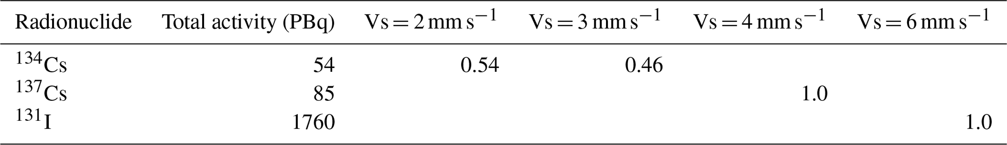
The ability to simulate the transport and deposition of radionuclides is a new feature in FALL3D-8.0. In order to simulate the dispersion of radioactive material, estimations of the emission rate and of the particle size distributions and settling velocities of radioactive material (e.g. ¹³⁴Cs, ¹³⁷Cs and ¹³¹I isotopes) are needed. Unfortunately, existing estimations of such parameters are uncertain due to obvious in situ measurement difficulties and to the interaction of isotopes with other atmospheric particles and aerosols (Brandt et al., 2002), and rely on reconstructions and/or on best fitting the available measurements in the region of interest at the time of the accident. For example, on the basis of high-quality deposition measurements from the REM database (De Cort et al., 2007), Brandt et al. (2002) reconstructed the source term and identified two emission phases with different vertical mass distributions. The Chernobyl-1986 test suite case uses the source term reported by Brandt et al. (2002), parameterised using the SUZUKI and HAT options in FALL3D (see Table 1 for more details of the input parameters). On the other hand, effective settling velocities typically range from 0.5 to 5 mm s⁻¹ for ¹³⁷Cs and from 1 to 20 mm s⁻¹ for ¹³¹I (Brandt et al., 2002). Considering these ranges and discretising velocities into four classes (see Table 5), we chose the effective classes and fractions for Chernobyl-1986 based on the best fit of the simulations with the measured deposit radioactivity on 10 May 1986. The best fit was performed by changing the nuclide size distribution (each class having a different settling velocity) and keeping the total mass constant. Minimisation was performed through a regular grid search varying the relative weights of the nuclide size classes between 0 and 1 at steps of 0.01. The Chernobyl-1986 case considers the computational domain shown in Fig. 8 for the period from 24 April to 10 May 1986, considering the input values reported in Table 5 and the meteorological fields obtained from ERA5 reanalysis, which accounts for atmospheric diffusion, wet deposition and radioactive decay.

Table 4 Summary of the SAL and FMS validation scores for the Puyehue-2011 and Raikoke-2019 test suite cases. The “DI” columns indicate validation scores for runs with data insertion and “NDI” indicates scores for runs with no data insertion.

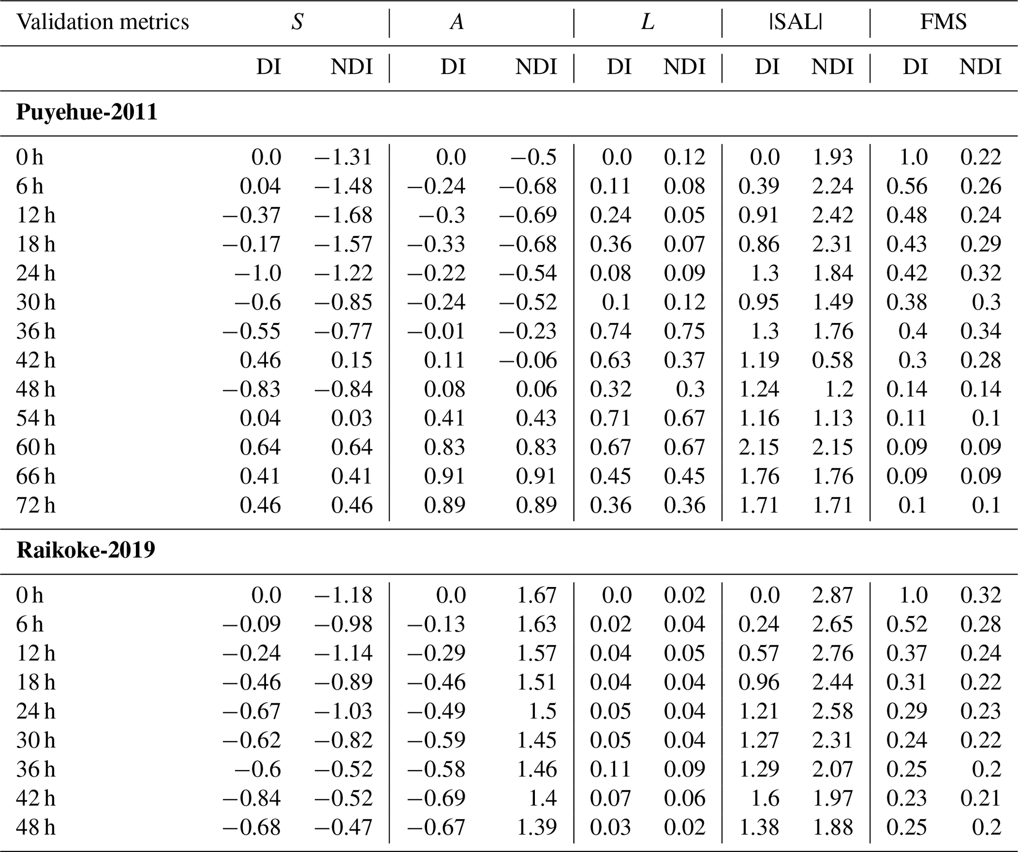
Table 5 Total radioactivity emitted in the atmosphere during the Chernobyl accident in the period 24 April–10 May 1986, for caesium and iodine isotopes, and their best fit fractions in the considered settling velocity classes.

4 Validation metrics

4.1 Structure, amplitude and location

Both qualitative and quantitative validation approaches have been used to validate previous versions of FALL3D against satellite observations (e.g. Corradini et al., 2011; Folch et al., 2012). The Puyehue-2011 and Raikoke-2019 test suite cases use the SAL metric (Wernli et al., 2008) to quantitatively compare satellite retrievals of volcanic ash and SO₂ to the corresponding simulations with and without data insertion. The SAL metric was originally developed for validation of precipitation forecasts against radar and satellite data (Wernli et al., 2008). However, Dacre (2011) demonstrated its use for validation of air pollution simulations, and Wilkins et al. (2016) employed the SAL for dispersion model validation against IR satellite volcanic ash retrievals for the 2010 Eyjafjallajökull eruption. More recently, the SAL has also been used to compare online vs. offline model simulations of volcanic ash (Marti and Folch, 2018). As in Wilkins et al. (2016) and Marti and Folch (2018), we also use the FMS score as a complement to SAL for comparing the spatial coverage of observed vs. modelled fields. A detailed mathematical description of the SAL metric is presented in Wernli et al. (2008), and so we only provide a brief description of each of the components of SAL (i.e. S, A and L) in the following subsections. The main requirement for calculating SAL is the determination of model and observation “objects”. Objects are identified as clusters of contiguous pixels whose magnitude is above some threshold corresponding to a physical quantity determined from observations. In our case, the threshold is determined based on the detection limit of the satellite retrievals. For the SEVIRI ash retrievals (Puyehue-2011 test suite case), we used a threshold of 0.2 g m⁻², consistent with the threshold suggested by Prata and Prata (2012). For the AHI SO₂ retrievals (Raikoke-2019 test suite case), there is currently no commonly accepted detection threshold. For the purposes of identifying SO₂ objects, we allowed for a threshold of 5 DU, noting that the minimum detected SO₂ total column burdens at each time step in the satellite retrievals were generally ∼ 8–10 DU. After identifying objects for both the observation (satellite retrievals) and model fields, we compute the SAL as the sum of the absolute values of S, A and L, which results in an index that varies from 0 (best agreement) to 6 (worst agreement). All comparisons between observations and model simulations were made using a regular 0.1^∘ × 0.1^∘ latitude–longitude grid.

4.1.1 Amplitude

The amplitude (A) metric is the simplest of the three SAL components and compares the normalised difference of the mass-averaged values of the observation and model fields. It can vary from −2 to +2, where negative (positive) values indicate that the model is underpredicting (overpredicting) the mass when compared with observations.

4.1.2 Location

The location (L) metric has two components ($L=L_{\mathrm{1}}+L_{\mathrm{2}}$). L₁ is calculated as the distance between the centres of mass between the model and observation objects, normalised by the maximum distance across the specified domain. It can vary from 0 to +1 and is considered a first-order indication of the accuracy of the model simulation compared with observations. However, L₁ can equal 0 (suggesting perfect agreement) for situations where observation and model fields clearly do not agree. For example, Wernli et al. (2008) describe the case of two objects at opposite sides of the domain having the same centre of mass as a single object in the centre of the domain. L₂ was introduced to handle these situations by considering the weighted average distance between the overall centre of mass and the centre of mass of each individual object for both model and observation fields. L₂ is computed by taking the normalised difference between the model weighted average distance and the observation weighted average distance. It is scaled such that it varies from 0 to +1 (to vary over the same range as L₁), meaning that L varies in the range from 0 to +2.

4.1.3 Structure

The structure (S) metric is the most complex of the three metrics used to construct SAL. The general idea is to compute the normalised “volume” of all individual objects for each dataset (i.e. the model and observation fields). The normalised volumes are computed by dividing the total (sum) mass of each object by its maximum mass. The weighted mean of the normalised volumes is then computed for the observation and model fields and S is computed by taking the difference between the weighted means. The S metric can vary from −2 to +2, where negative values indicate that modelled objects are too small or too peaked (or a combination of both) compared to the observed fields.

4.2 Figure of merit in space

The FMS score compares the spatial coverage of observed vs. modelled fields. It is simply the area of intersection divided by the area of union between the ash mass loading observation and model fields:

$$\begin{array}{}\text{(2)}& \text{FMS}={\displaystyle \frac{A_{\text{mod}}\cap A_{\text{obs}}}{A_{\text{mod}}\cup A_{\text{obs}}}},\end{array}$$

where A_mod and A_obs are the modelled and observed ash mass loading areas, respectively. The FMS varies from 0 (no intersection) to 1 (perfect overlap).

4.3 Root-mean-square error

The Etna-2013 and Chernobyl-1986 test suite cases use the RMSE metric to quantitatively compare observations and numerical simulations. For this purpose, we consider two variants of the normalised RMSE, defined as (Poret et al., 2018)

$$\begin{array}{}\text{(3)}& \begin{array}{rl}& {\mathrm{RMSE}}_j=\sqrt{\sum _i^N{w}_j({\text{MOD}}_i-{\text{OBS}}_i{)}^{\mathrm{2}}}\\ & \text{with}\\ & w_{\mathrm{1}}={\displaystyle \frac{\mathrm{1}}{{\sum }_i^N{\text{OBS}}_i^{\mathrm{2}}}}\\ & w_{\mathrm{2}}={\displaystyle \frac{\mathrm{1}}{N}}{\displaystyle \frac{\mathrm{1}}{{\text{OBS}}_i^{\mathrm{2}}}},\end{array}\end{array}$$

where $j=\mathrm{1},\mathrm{2}$ depends on the RMSE choice, w_j refers to the weighting factor used to normalise RMSE, and OBS_i and MOD_i are the observed and modelled mass loading related to the ith sample over a set of N samples. The weights correspond to different assumptions about the error distribution (e.g. Aitken, 1935; Costa et al., 2009). RMSE₁ calculated with w₁ refers to a constant absolute error, whereas RMSE₂, calculated using a proportional weighting factor w₂, considers a constant relative error (e.g. Bonasia et al., 2010; Folch et al., 2010; Poret et al., 2018).

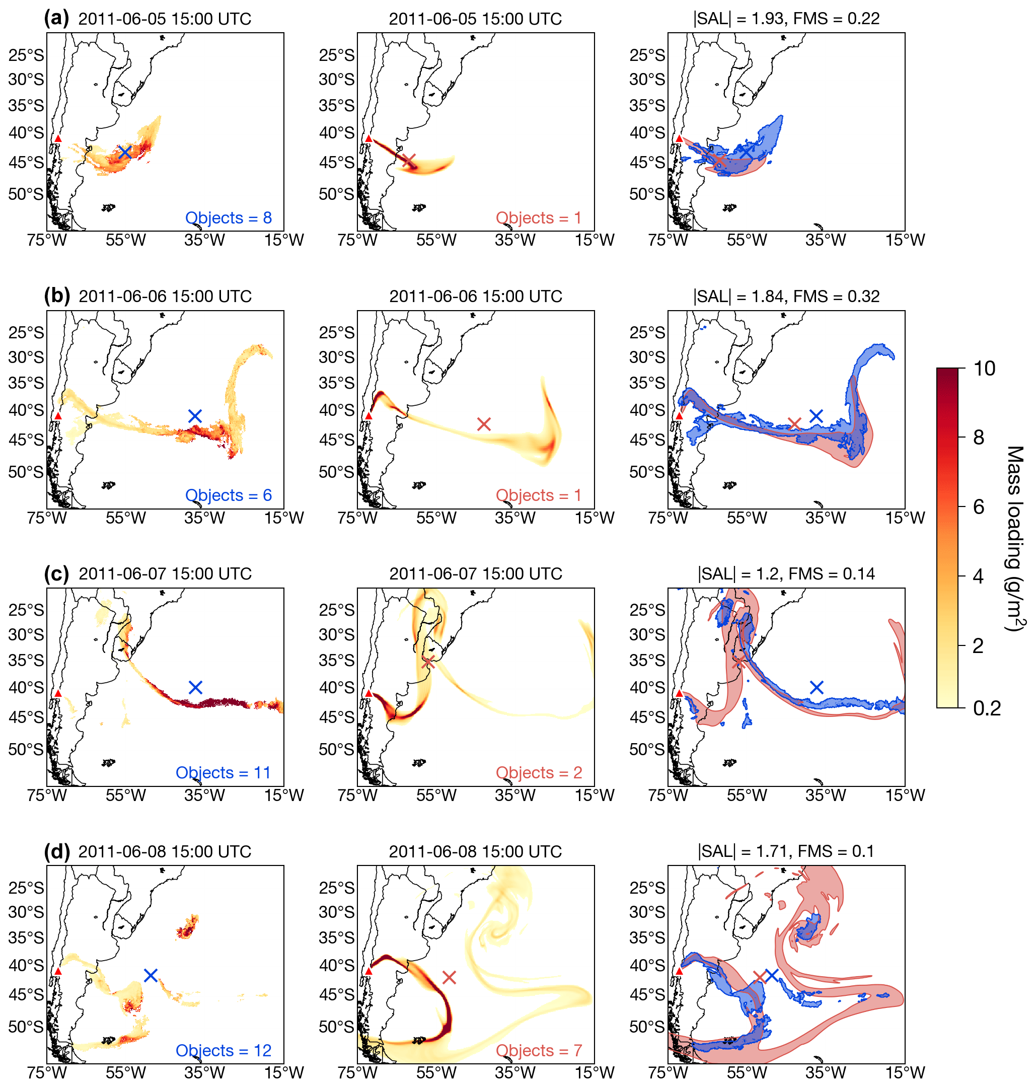
Figure 2 Same as Fig. 1 but without data insertion.

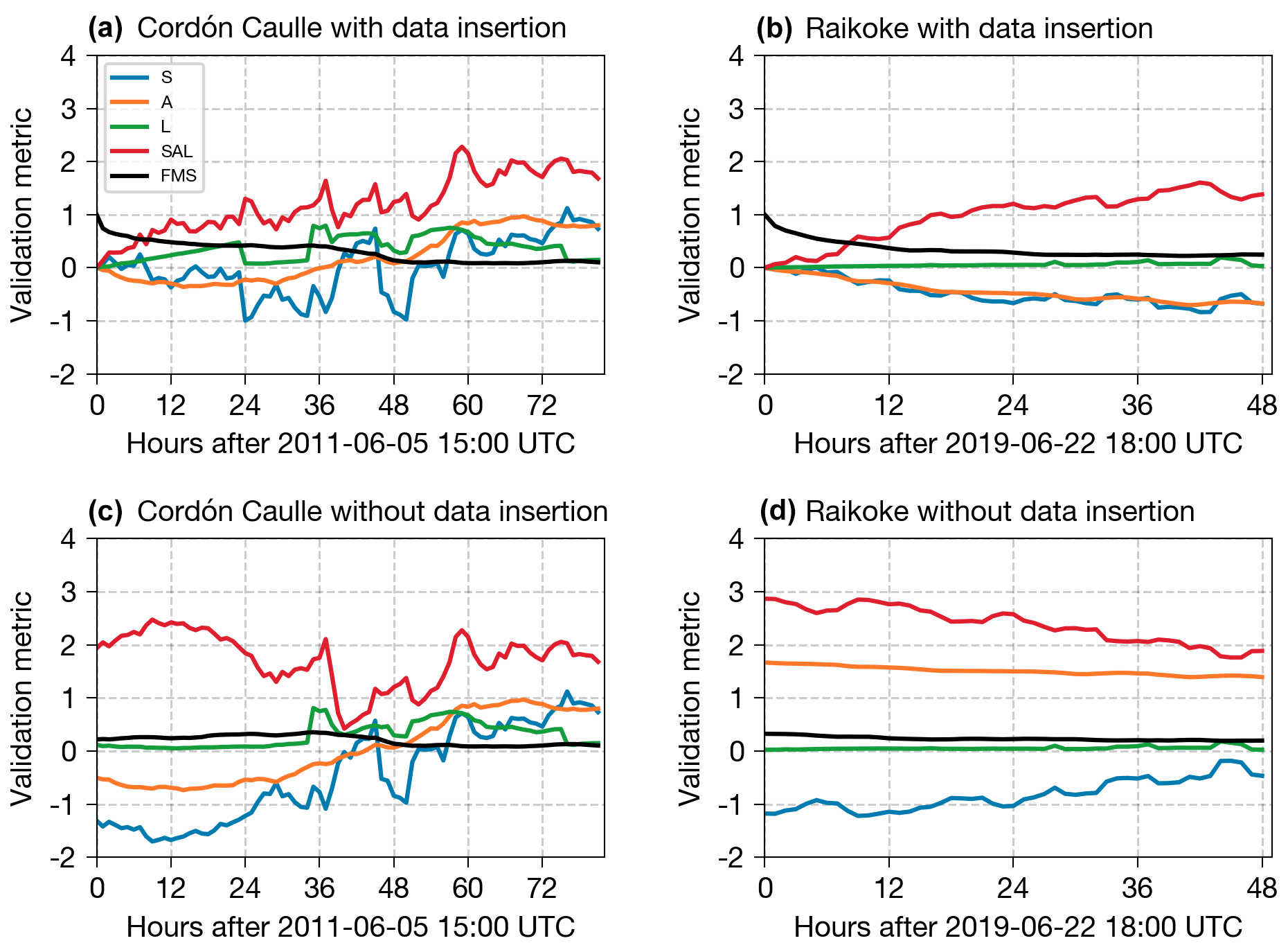
Figure 3 Time series of validation metrics for (a) Puyehue-2011 test case with data insertion, (b) Raikoke-2019 test case with data insertion, (c) Puyehue-2011 without data insertion, and (d) Raikoke-2019 without data insertion.

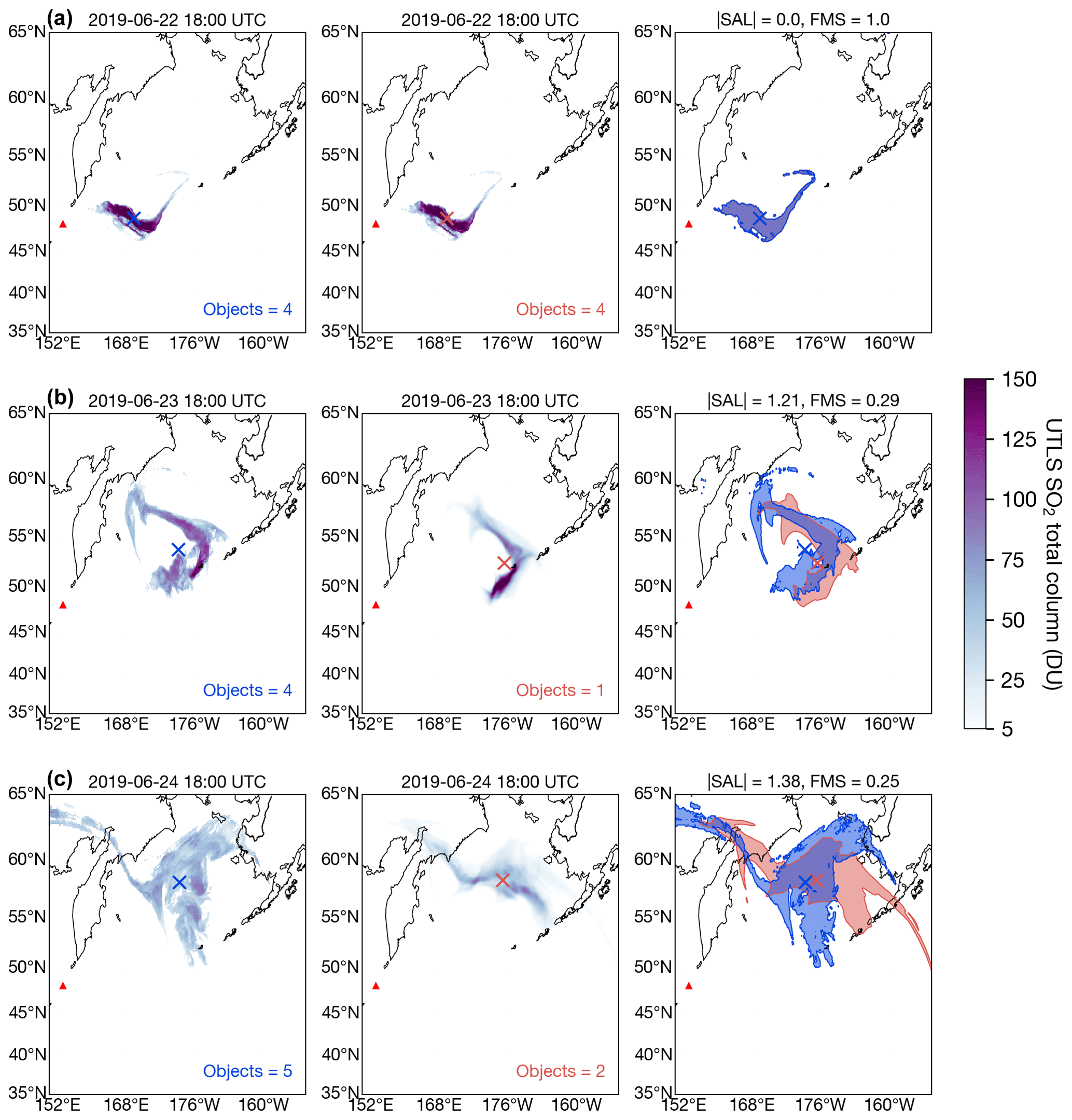
Figure 4 Raikoke-2019 validation test results using AHI upper troposphere–lower stratosphere (UTLS) total column burdens retrievals (DU) on (a) 22 June 2019 at 18:00 UTC (data insertion time), (b) 23 June 2019 at 18:00 UTC and (c) 24 June 2019 at 18:00 UTC. Left column shows satellite retrievals with 5 DU contour in blue and centre of mass indicated with an “x”. Middle column shows FALL3D model simulation (5 DU contour in red). Right column shows spatial overlap of model (shaded in red) vs. observed (shaded in blue) fields. A full animation of the data insertion simulations is available in the Video Supplement 2 (Prata et al., 2020b).

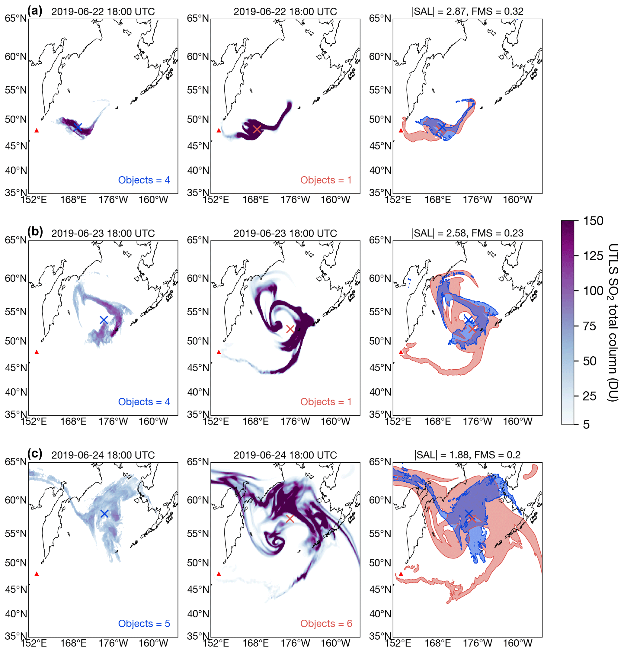
Figure 5 Same as Fig. 4 but without data insertion.

5 Validation results

5.1 Puyehue-2011

Figures 1 and 2 compare satellite retrievals and model simulations for the Puyehue-2011 case at the data insertion time (15:00 UTC on 5 June 2011) as well as 24, 48 and 72 h after the insertion time for runs with and without data insertion, respectively. The time series of each validation metric are also shown in Fig. 3a, c and summarised in Table 4. Comparison of Figs. 1a and 2a highlight the advantage of a data insertion scheme to specify model initial conditions. Note that for simulations with data insertion at the data insertion time the validation metrics reflect perfect scores (i.e. SAL of 0 and FMS of 1). For the simulation without data insertion (Fig. 2a), the plume has already begun to deviate from the satellite observations with too much mass dispersing towards the south. This is reflected in both the SAL score of 1.93 and FMS score of 0.22 at this time. The data insertion scheme (Fig. 1a) naturally corrects for this by taking advantage of good-quality satellite observations of the vertical and horizontal structure of the Puyehue ash plume at the insertion time. For the data insertion simulations, FALL3D accurately represents the spatial structure of the satellite retrievals after 24 h with a SAL score of 1.3 and FMS of 0.42 (Fig. 1b; see the Video Supplement (Prata et al., 2020a) for the full animation of the data insertion simulations). In addition, the accuracy of the simulations over the first 24 h shows a marked improvement when compared to the simulations without data insertion (Fig. 2b; SAL of 1.84; FMS of 0.32). The validation metric time series show this in more detail (Figs. 3a and b). For the simulations without data insertion, the SAL score remains above 2 for most of the first 24 h, while it gradually increases from 0 to 1.3 for the simulation with data insertion. Comparison of Figs. 1b and  2b shows that the data insertion simulation is better able to capture the northern portion of the plume than the simulation without data insertion at this time (an increase in the FMS by 0.1). Inspection of the time series of the individual validation metrics for the simulations with data insertion (Fig. 3a) reveals that the SAL is largely being affected by increases in the L metric (i.e. increases in the distance between the centres mass between the observation and model fields) and decreases in the A metric (model underpredicting mass compared to observations). The S metric only exhibits minor deviations when compared to the observations during the first 24 h after data insertion. At 48 h, the simulations with and without the data insertion are almost identical (minor differences in the modelled ash contours near 30^∘ S, 15^∘ W). This is because, at this time, almost all of the ash used in the data insertion has exited the domain. For the simulations without data insertion, the SAL score is 1.2 and FMS is 0.14 (Fig. 2c; Table 4); however, at around 36 h, SAL reached above 2 and then decreased sharply (Fig. 3c). The reason for the sudden reduction in SAL just after 36 h is most likely due to the satellite retrievals being compromised by cloud interference at this time in addition to the continual input of mass due to the emission source in the model simulations. Note that this input of mass was included to account for ash erupted after the data insertion time. The satellite retrievals capture some of the ash plume near the source (Figs. 1c and 2c) but cannot be expected to accurately characterise the plume at this location due to its high opacity in the IR window. Another difference between the model and observations at this time is the large difference in the centres of mass (L=0.32). This is due to the high mass loadings near source in the model fields and high mass loadings near the centre of the domain (43^∘ S, 35^∘ W) in the observed fields. The satellite is likely overestimating mass in this part of the ash cloud because of underlying water and/or ice clouds that have not been accounted for in the radiative transfer modelling. Simulations with and without data insertion are identical after 72 h as all ash used in the data insertion scheme has exited the domain (Figs. 1d and 2d). At this time, the SAL reached a score of 1.71 and the FMS has decreased to 0.10, reflecting a model predictive performance degrading over time.

5.2 Raikoke-2019

Figures 4 and 5 show a comparison between the satellite retrievals and model simulations with and without data insertion, respectively, in addition to the SAL and FMS validation metrics. The time series of validation metrics for the Raikoke-2019 case are shown in Fig. 3b and d and are summarised in Table 4. The AHI retrievals of the SO₂ plume at the beginning of the eruption (Fig. B3a) were likely compromised by interference of ice particles in the initial eruption plume (Prata et al., 2003; Doutriaux-Boucher and Dubuisson, 2009). In addition, retrievals early on in the plume's dispersion may have been affected by band saturation caused by extremely high SO₂ column loads. At the data insertion time (22 June 2019 at 18:00 UTC), the SAL score for the SO₂ simulation without data insertion is 2.87 and the FMS is 0.32. Therefore, applying data insertion at this time represents a significant correction to the model simulation when compared against the satellite retrievals (compare Figs. 4a and 5a). The main difference between the satellite retrievals and simulation without data insertion is that the model indicates a portion of the SO₂ plume connecting back to the volcano, while this feature is not present in the observations. TROPOMI observations of the SO₂ cloud confirm this spatial structure (see Fig. 13 of Global Volcanism Program, 2019) and highlight the importance of understanding the limitations of the AHI retrievals used for data insertion in the present study. The reason for the lack of detection of SO₂ in this region in the AHI retrievals is probably due to water vapour interference, implying that this part of the plume was at lower altitudes than the main SO₂ cloud. Indeed, SO₂ height retrievals from CrIS data show that plume heights varied from ∼ 3 to 7 km a.s.l. in this region (see Fig. 5 of Hyman and Pavolonis, 2020).

For the simulations without data insertion, at 24 h after insertion, the validation metrics exhibit minor changes with SAL decreasing from 2.87 to 2.59 and the FMS from 0.32 to 0.23 (Fig. 5a, b). For the simulations with data insertion, SAL has steadily increased from 0 to 1.21, while the FMS has decreased from 1 to 0.29 over the first 24 h (Fig. 4a, b; see the Video Supplement, Prata et al., 2020b, for the full animation of the data insertion simulations). Figure 3b shows that the SAL score for the simulation with data insertion is mostly affected by the S and A scores, whereas the L score is low (0.05) indicating that FALL3D is able to track the centre of mass of SO₂ very well when initialised with satellite retrievals (Fig. 3b). In this case, the A metric is negative, meaning that the model is underpredicting the mass when compared to the satellite retrievals. Given that FALL3D-8.0 does not include SO₂ chemistry and only includes SO₂ deposition mechanisms (Folch et al., 2020), it is unlikely that the model is losing SO₂ mass too rapidly. Instead, this underprediction is probably being driven by the observed increase in mass retrieved by the satellite after the insertion time, which cannot be accounted for in the data insertion scheme if no new sources of SO₂ are included in the model simulations. An increase in mass, even after the SO₂ cloud has detached from source, could be related to the detection sensitivity of the satellite retrieval and the influence of water vapour (Prata et al., 2003; Doutriaux-Boucher and Dubuisson, 2009). For example, if the SO₂ cloud is in a region of high water vapour initially and then moves into a drier region, it is possible that more SO₂ will be detected thus increasing the retrieved mass. This effect could also occur if the SO₂ layers are transported vertically in the atmosphere. Another interesting mechanism for the observed increase in SO₂ mass after the plume has detached from source is ice–SO₂ sequestration. This phenomenon occurs when ice particles in the nascent plume sequester SO₂ initially and then release it later on as the ice sublimates in the UTLS (e.g. Rose et al., 2001, 2003, 2004; Guo et al., 2004; Prata et al., 2007; Fisher et al., 2019).

At 48 h, for the simulations without data insertion (Fig. 5c), the SAL score actually improves (decreasing from 2.58 to 1.88) and the FMS largely remains the same (decreasing from 0.23 to 0.20). The improvement in the SAL score can be attributed to a steady increase in S metric and decrease in the A metric (Fig. 3d). This indicates that the structure and mass (amplitude) simulated without data insertion are converging towards that observed by the satellite over 48 h. For the simulations with data insertion, 48 h after insertion (Fig. 4c), the SAL score continues to increase (from 1.21 to 1.38) and the FMS continues to decrease (from 0.29 to 0.25). In general, at all lead times, the validation metrics indicate that the data insertion simulations provide better agreement with observations than the simulations without data insertion (Table 4).

5.3 Etna-2013

Figure 7a compares modelled and observed tephra loading for the 2013 Mt. Etna eruption at all observation sites (detailed in Sect. 3.3.1). Note that all points are found within a factor of 3 around the perfect agreement line (solid black line) across 4 orders of magnitude (from 10⁻³ kg m⁻² to more than 10 kg m⁻²). This good agreement is also observed at a bin level in the local grain size distributions. According to the model predictions presented here, unimodal local distributions (negligible ash aggregation effects) are found at all sampling sites, in good agreement with field observations (Poret et al., 2018). In addition, variations of the grain size distribution were accurately captured by the simulations as shown in Fig. 7b, which compares computed and observed particle distribution modes at all sites (S1–S10).

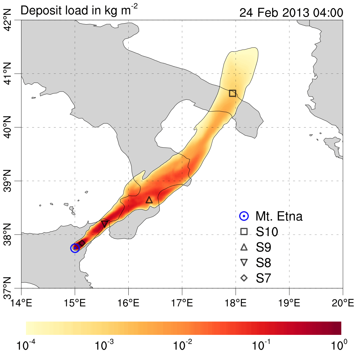
Figure 6 Tephra fallout deposit from the Etna-2013 test case. The spatial distribution of the modelled tephra loading coincides with the locations of sampling sites. Sites S7–S10 are indicated on the map by symbols. Proximal sites S1–S6 (<16 km from the source) are not shown for clarity.

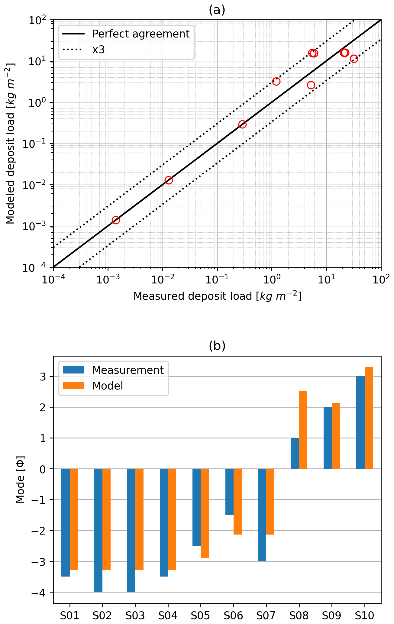
Figure 7 Comparison between field data at 10 sampling sites (S1–S10) and results from the Etna-2013 test case. (a) Tephra mass loading. (b) Mode of the distributions. Field data were obtained from the sample dataset reported by Poret et al. (2018).

In terms of the normalised RMSE (see Sect. 4.3), the model results presented here show a marked improvement compared to the FALL3D-7.3 results reported by Poret et al. (2018). In fact, RMSE₁ and RMSE₂ reduce from 0.7 and 2.84 in Poret et al. (2018) to 0.58 and 0.98 in this study. The main differences between the simulations performed by Poret et al. (2018) and this study can be attributed to (i) the horizontal resolution of both the meteorological input data and the dispersal model; (ii) the vertical coordinate system; (iii) the TGSD used to define the source term; and (iv) the dry deposition parameterisation. Specifically, higher resolution simulations along with the improved numerical scheme implemented in FALL3D-8.0 are expected to lead to a reduction of numerical diffusion errors, which is clearly manifested in the spatial distribution of the tephra mass loading field (compare Fig. 6 in the present study to Fig. 6 in Poret et al., 2018). A volcanic ash mass loading simulation for the Etna-2013 test suite case is available in the Video Supplement 3 (Prata et al., 2020c).

5.4 Chernobyl-1986

Validation for the 1986 Chernobyl nuclear accident was carried out using the normalised RMSE with a constant absolute error (i.e. RMSE₁ with w₁). Since the measured radioactivity spans over 4 orders of magnitude, the RMSE₁ was calculated between the logarithms of the measured and modelled radioactivity values at different tracking points (29 for ¹³¹I, 44 for ¹³⁴Cs and 45 for ¹³⁷Cs, from the REM database). The obtained values of RMSE₁ are 0.10, 0.09 and 0.06 for ¹³¹I, ¹³⁴Cs and ¹³⁷Cs, respectively. A map showing the ¹³⁷Cs deposit distribution simulated can be found in Fig. 8. The comparison of measured and simulated values for the best fitted terminal velocity bins (Table 5) is shown in Fig. 9. Note that most of simulated values lie within an order of magnitude of the measurements (Fig. 9). Simulation results of the radioactive cloud evolution relative to ¹³⁷Cs (vertically integrated radioactivity concentration in the atmosphere, expressed in Bq m⁻²) from 28 April to 9 May 1986, are shown in Fig. 10. Figure 10 shows that the Chernobyl-1986 simulations correctly reproduce the patterns described by Brandt et al. (2002). The evolution of the ¹³⁷Cs dispersal is also available as a video in the Video Supplement 5 (Prata et al., 2020e), together with videos corresponding to the dispersal of ¹³⁴Cs (Video Supplement 4; Prata et al., 2020d) and ¹³¹I (Video Supplement 6; Prata et al., 2020f).

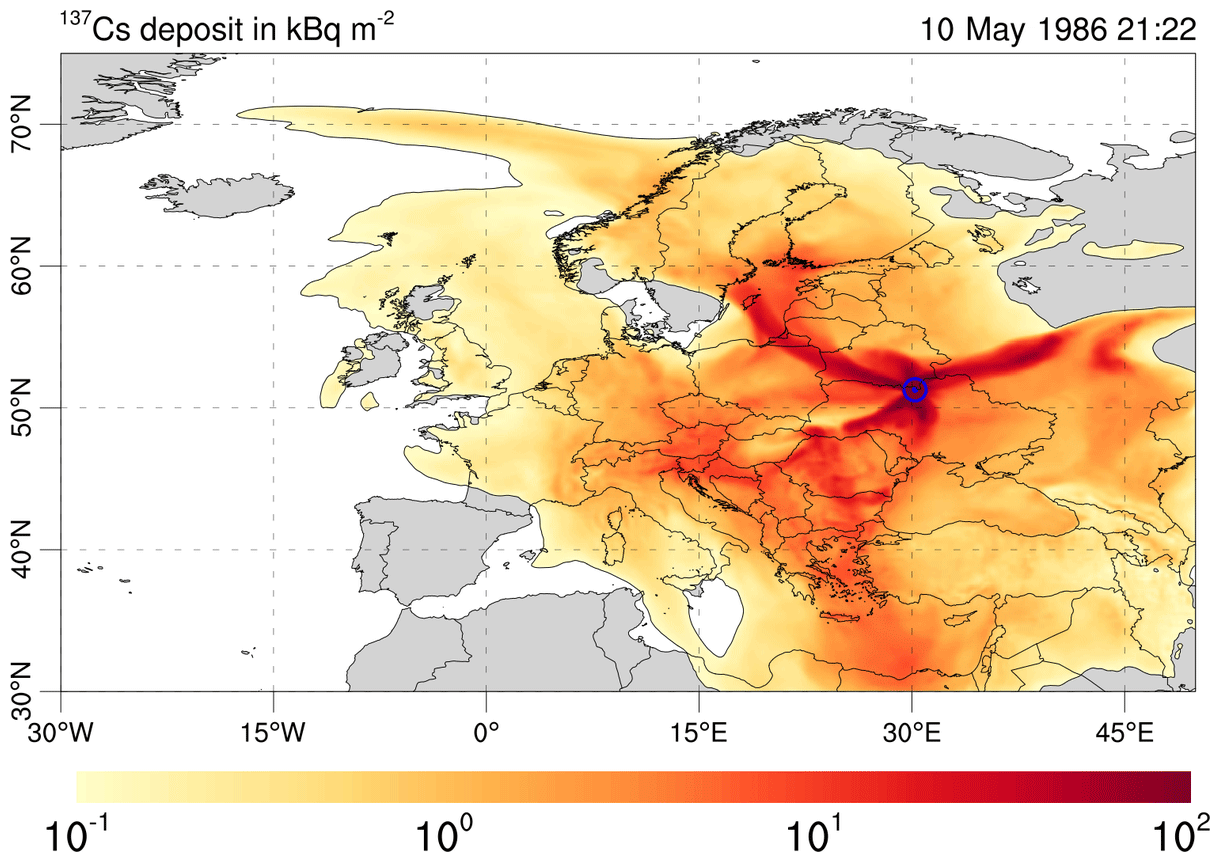
Figure 8 Chernobyl-1986 accumulated total deposition of ¹³⁷Cs on 10 May 1986. The underlying map is reported just for reference and could contain nations' borders that are under dispute.

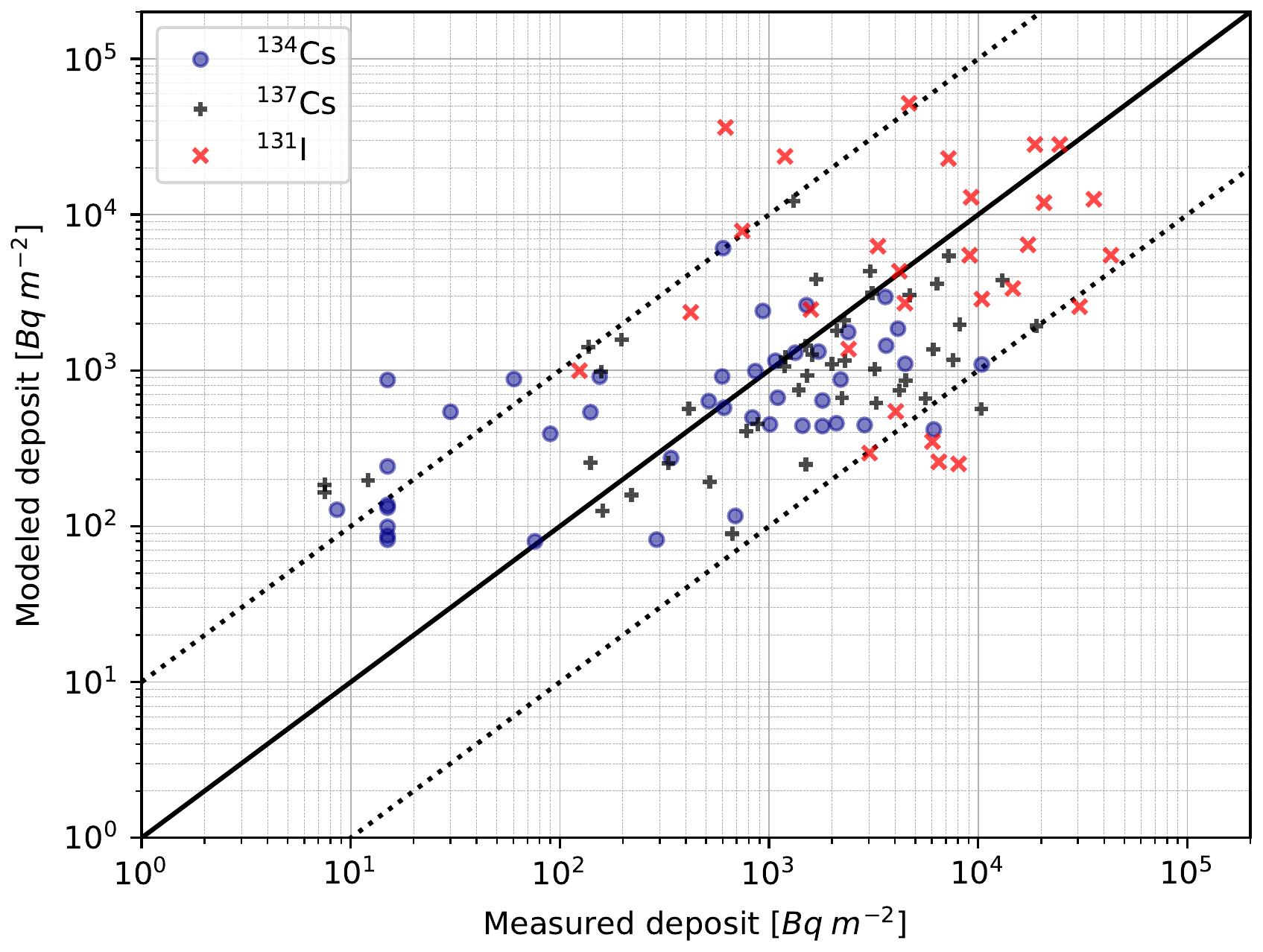
Figure 9 Comparison between measurements and Chernobyl-1986 test deposit results of ¹³⁷Cs, ¹³⁴Cs and ¹³¹I at different locations on 10 May 1986. The solid line represents one-to-one agreement between measured and modelled values. Lower and upper dashed lines represent factors of 0.1 and 10, respectively, from the one-to-one line.

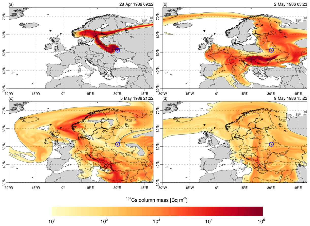
Figure 10 Vertically integrated ¹³⁷Cs radioactivity concentration in the atmosphere at different times according to Chernobyl-1986 test results: (a) 28 April 1986, (b) 2 May 1986, (c) 5 May 1986 and (d) 9 May 1986. The underlying maps are reported just for reference and could contain nations' borders that are under dispute.

6 Conclusions

Four different examples from the new FALL3D-8.0 benchmark suite have been presented to validate the accuracy of the latest major version release of the FALL3D model and complement a companion paper (Folch et al., 2020) on model physics and performance. In the first two examples, geostationary satellite observations from Meteosat-9 (SEVIRI) for the 2011 Puyehue-Cordón Caulle eruption (i.e. Puyehue-2011 test suite case) and from Himawari-8 (AHI) for the 2019 Raikoke eruption (i.e. Raikoke-2019 test suite case) were used to validate FALL3D simulations of far-range fine ash dispersal and SO₂ cloud dispersal, respectively. The metrics used for validation were the SAL and FMS and were applied to simulations with and without data insertion. To characterise the vertical structure of these volcanic clouds at selected data insertion times, geostationary satellite observations were collocated with CALIPSO overpasses. According to the SAL and FMS metrics, simulations initialised with data insertion consistently outperform simulations without data insertion. For the data insertion simulations, SAL remained below 1 out to 18 h (Table 4) and below 2 at lead times of 24 and 48 h for both ash and SO₂ simulations. While it is not yet clear what absolute values of SAL and FMS should represent an acceptable ash∕SO₂ forecast, it is unlikely that in an operational setting a model simulation would be relied upon beyond 48 h. Ideally, the model should be re-run with an updated data insertion time when new, good-quality satellite retrievals become available. Based on our findings, it appears that SAL values of less than 1.5 and FMS values greater than 0.40 indicate good spatial agreement between the model and observation fields (e.g. Fig. 1b). However, it is important to consider that the satellite retrievals can be affected by several factors (e.g. cloud interference, high water vapour burdens, chosen detection thresholds) meaning that the ash∕SO₂ detection schemes may miss some legitimate ash or SO₂ that the model is otherwise predicting (e.g. Fig. 1c). Limitations of the observations should also be taken into account when initialising simulations with data insertion. A data assimilation scheme that considers the errors in the satellite retrievals in addition to errors in the model simulations (e.g. using an ensemble approach to generate probabilistic forecasts) can be used to resolve these issues (e.g. Fu et al., 2017; Pardini et al., 2020).

For the Etna-2013 test suite case, very good agreement between field observations and simulations of deposit loads was found. This is evidenced by the fact that acceptable ratios of model to observed ash loading (between 1:3 and 3:1) exist across 4 orders of magnitude (i.e. from 10⁻³ kg m⁻² to more than 10 kg m⁻²). Good agreement in terms of the local grain size distributions was also found for all sampling sites, as can be seen by comparing the simulated and observed mode of each distribution (Fig. 6b). Quantitative comparisons using normalised RMSE metrics have shown that the results of the present work have outperformed previous studies based on prior versions of FALL3D (version v7.3 or older). This is a direct consequence of multiple improvements incorporated in the new release of FALL3D (version v8.0), including a new numerical scheme and a new vertical coordinate system. Additionally, improvements in terms of code parallelism, memory management, model performance and scalability allow for higher resolution simulations and a more realistic modelling.

For the Chernobyl-1986 test suite case, very good agreement between the model simulations and observations was found for the dispersal of radioactivity (i.e. ¹³¹I, ¹³⁴Cs and ¹³⁷Cs) resulting from the 25 April 1986 Chernobyl nuclear accident, consistent with the findings of Brandt et al. (2002).

Future developments of the test suite include adding more case studies, model intercomparison studies that make use of the validation datasets provided here and validation of probabilistic forecasts. In terms of model utilities, we plan to introduce the option of ensemble forecasts and to incorporate data assimilation in future versions of FALL3D.

Appendix A: Volcanic ash retrieval

Satellite detection of volcanic ash using passive IR brightness temperature differences (BTDs) between channels centred around 11 and 12 µm has been widely used for more than 30 years (Prata, 1989a, b). Quantitative ash retrievals based on the BTD method have also been practiced for a long time (e.g. Wen and Rose, 1994; Prata and Grant, 2001) and the uncertainties stemming from detection (e.g. Simpson, 2000; Prata et al., 2001) and radiative transfer modelling (e.g. Wen and Rose, 1994; Corradini et al., 2008; Kylling et al., 2014; Stevenson et al., 2015; Western et al., 2015) are well known. Figure A1 shows SEVIRI observations of the Cordón Caulle volcanic ash plume and illustrates the steps used to detect volcanic ash in the present study. For context, Fig. A1a and b show a composite of MODIS True Color imagery and the SEVIRI 10.8 µm brightness temperature ($T_{\mathrm{B}}^{\mathrm{11}}$), respectively. Here, we propose an ash detection scheme based on applying successive masks that flag SEVIRI pixels as “ash affected” before attempting a subsequent quantitative ash retrieval:

1. First, we apply a temperature cut-off threshold to water-vapour-corrected BTDs (ΔT_ash):

   $$\begin{array}{}\text{(A1)}& \mathrm{\Delta }{T}_{\text{ash}}=T_{\mathrm{B}}^{\mathrm{11}}-T_{\mathrm{B}}^{\mathrm{12}}<T_{\mathrm{wc}};\end{array}$$

   that is, only those pixels with ΔT_ash less than the cut-off threshold of $T_{\mathrm{wc}}=-\mathrm{0.5}$ K are flagged as potential ash pixels. This water vapour correction follows the semi-empirical approach of Yu et al. (2002). As illustrated in Fig. A1c, this first threshold is reasonably effective at detecting the Cordón Caulle ash cloud. However, this simple cut-off threshold may not remove false positives due to temperature inversions generated by clear land at night (Platt and Prata, 1993), ice-covered surfaces (Yamanouchi et al., 1987), cold cloud tops (Potts and Ebert, 1996) and high satellite zenith angles (Gu et al., 2005).

2. Second, we apply a cold surface mask designed to remove false positives due to reasons mentioned above. This cut-off condition relabels potential ash pixels as “ash free” if

   $$\begin{array}{}\text{(A2)}& \mathrm{\Delta }{T}_{\text{ash}}>T_{\mathrm{sc}}\text{ and}\left\{\begin{array}{l}{T}_{\mathrm{B}}^{\mathrm{11}}>\mathrm{255}\mathrm{K}\text{ over land}\\ T_{\mathrm{B}}^{\mathrm{11}}>\mathrm{240}\mathrm{K}\text{ over ocean},\end{array}\right.\end{array}$$

   where $T_{\mathrm{sc}}=-\mathrm{1.5}$ K is the cold surface cut-off value. We note that $T_{\mathrm{B}}^{\mathrm{11}}$ condition of this mask will preserve ash detection sensitivity for high-altitude (cold) ash clouds, which is particularly well suited for the Cordón Caulle case study. However, this condition may not be suitable for low-level ash clouds (low thermal contrast resulting in less negative BTDs in addition to warmer cloud tops). The effect of this mask is illustrated by comparing Fig. A1c and d. Note how, for the case shown, the cold surface mask removes almost all false positives over the region covered by low-level stratiform clouds.

3. Third, we apply a mask for false positives due to an increased path length at high satellite zenith angles (Gu et al., 2005). We mask out false positives at high zenith angles imposing

   $$\begin{array}{}\text{(A3)}& \mathrm{\Delta }{T}_{\text{ash}}>T_{\mathrm{zc}}\text{ and }\mathit{\zeta }>\mathrm{80}{}^{\circ },\end{array}$$

   where $T_{\mathrm{zc}}=-\mathrm{2}$ K is the zenith cut-off threshold and ζ is the satellite zenith angle. The effect of the high zenith mask can be seen by comparing Fig. A1d and e.

4. Finally, the last step in the detection process is to remove any spurious ash-labelled pixels using a noise filter that removes objects (groups of contiguous pixels) that are less than 16 pixels in size (Fig. A1f).

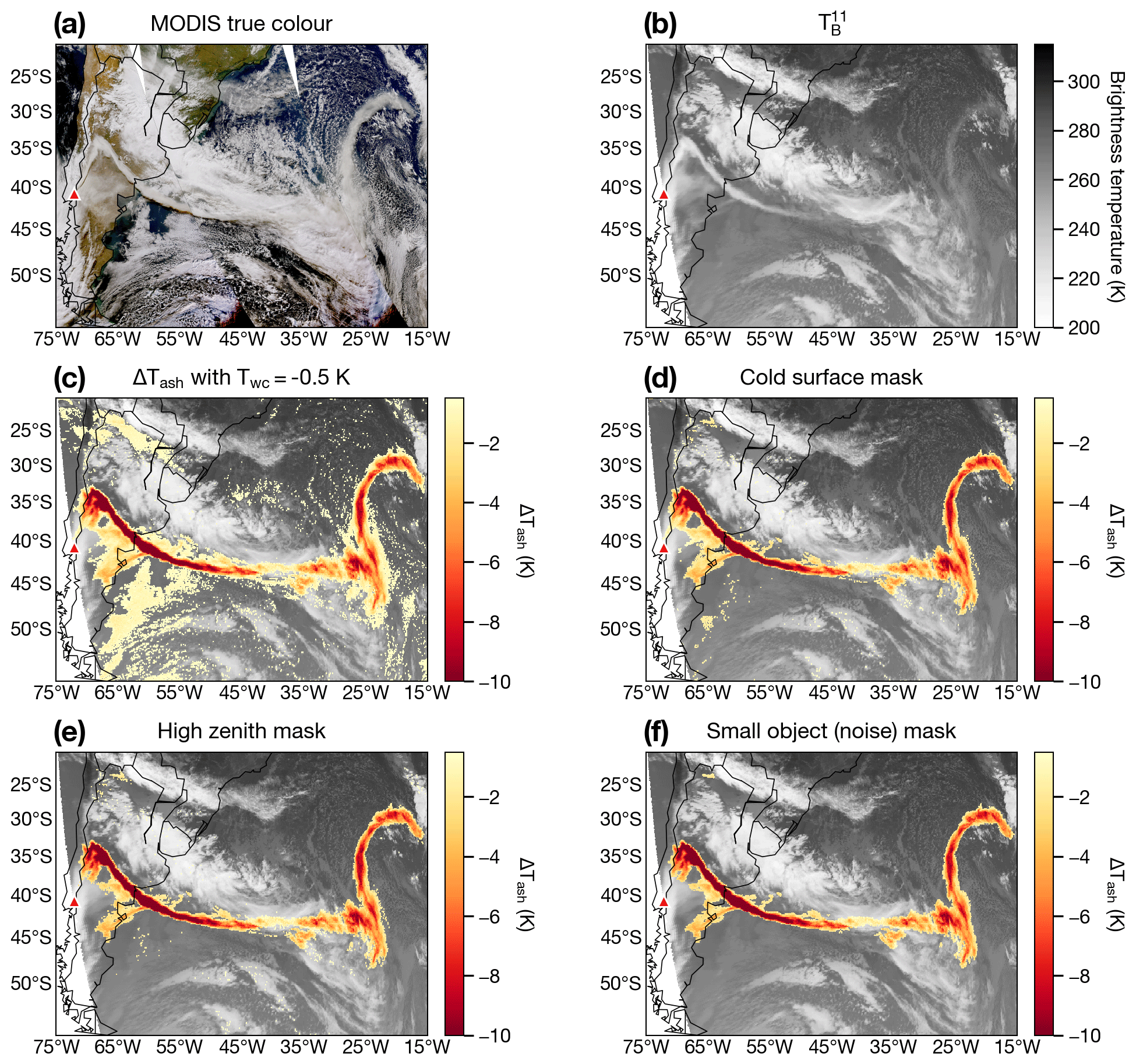
Figure A1 Volcanic ash detection scheme for the Puyehue-Cordón Caulle (indicated by the triangle on each map) eruption. (a) MODIS True Color composite from 6 June 2011 at 15:15–18:40 UTC. (b) SEVIRI 10.8 µm brightness temperature ($T_{\mathrm{B}}^{\mathrm{11}}$) on 6 June 2011 at 18:45 UTC. (c) Same as panel (b) with water-vapour-corrected BTD ($\mathrm{\Delta }{T}_{\text{ash}}=T_{\mathrm{B}}^{\mathrm{11}}-T_{\mathrm{B}}^{\mathrm{12}}$) overlaid. Panels (d), (e) and (f) are the same as (c) with cold surface, high zenith and noise masks applied, respectively.

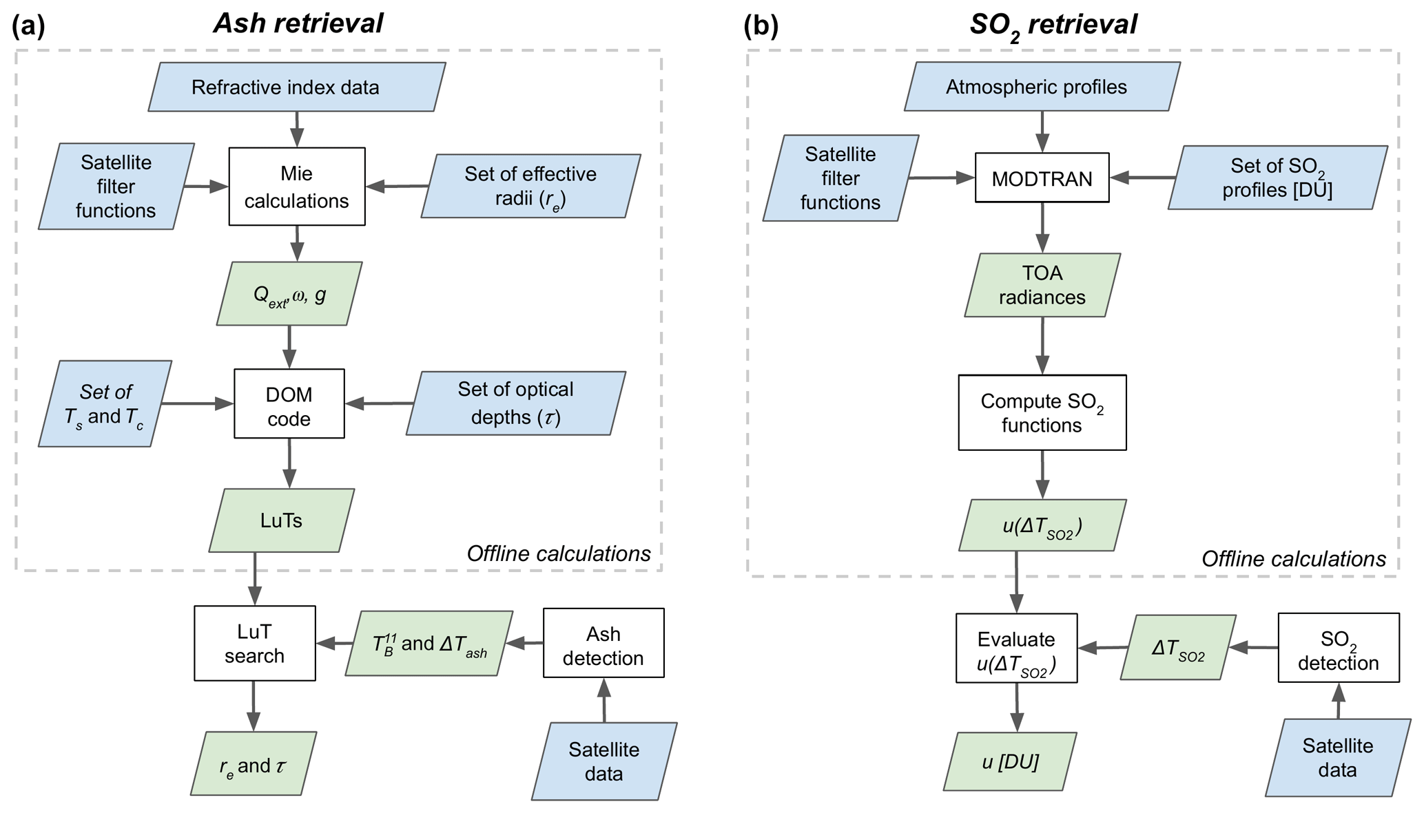
Figure A2 Flow diagram showing the (a) volcanic ash retrieval process and (b) volcanic SO₂ retrieval process used in the present study. Parallelograms indicate datasets (blue for inputs, green for outputs) and rectangles indicate processes (i.e. code used to implement the retrieval algorithms and perform radiative transfer calculations). Offline calculations are any computations that are precomputed (i.e. before any observations are made by the satellite).

The MODIS True Color composite shown in Fig. A1a illustrates that, even in a relatively complex scene (numerous clouds, large regions of land and ocean, high mountains, ice-covered surfaces, etc.), the ash detection is robust and provides a good balance between reduced false positives and increased true positives. An interesting point to note is that negative BTDs in the vicinity of Cordón Caulle are enhanced due to the high satellite zenith angles at these locations. Gu et al. (2005) discuss the benefit of improved sensitivity to ash at high satellite zenith angles but also show that mass loading retrievals can be overestimated in these situations. We correct for the effect of high zenith angles after retrieving the mass loading. Once pixels have been identified as being “ash affected”, we apply a look-up table (LuT) approach (Prata and Grant, 2001; Prata and Prata, 2012) to retrieve volcanic ash optical depth (τ), effective radius (r_e; in µm) and column mass loading (m_l; in g m⁻²). The retrieval procedure is illustrated in Fig. A2a. The temperature difference model employed here is based on the forward model developed by Prata (1989b) and Wen and Rose (1994):

$$\begin{array}{}\text{(A4)}& I\left(\mathit{\lambda }\right)\approx e^{-\mathit{\tau }\left(\mathit{\lambda }\right)}B\left(T_{\mathrm{s}}\right)+\left(\mathrm{1}-e^{-\mathit{\tau }\left(\mathit{\lambda }\right)}\right)B\left(T_{\mathrm{c}}\right),\end{array}$$

where I(λ) is the radiance at the top of the atmosphere at wavelength (λ), τ(λ) is the wavelength-dependent optical depth, B(T_s) is the Planck radiance evaluated for surface temperature (T_s) below the ash cloud, and B(T_c) is the Planck radiance corresponding to the temperature at the ash cloud top (T_c). The optical depth is defined as

$$\begin{array}{}\text{(A5)}& \mathit{\tau }\left(\mathit{\lambda }\right)=\mathit{\pi }L\underset{\mathrm{0}}{\overset{\mathrm{\infty }}{\int }}{r}^{\mathrm{2}}{Q}_{\mathrm{ext}}(\mathit{\lambda },r)n\left(r\right)\mathrm{d}r,\end{array}$$

where L is the geometric thickness of the ash cloud, Q_ext(λ,r) is the extinction efficiency factor (determined from Mie calculations), r is the particle radius, and n(r) represents the distribution of particles within the ash cloud. The ash mass loading is determined as

$$\begin{array}{}\text{(A6)}& m_{\mathrm{l}}={\displaystyle \frac{\mathrm{4}}{\mathrm{3}}}\mathit{\rho }{\displaystyle \frac{r_{\mathrm{e}}\mathit{\tau }\left(\mathit{\lambda }\right)}{Q_{\mathrm{ext}}(\mathit{\lambda },r_{\mathrm{e}})}}\cos \left(\mathit{\zeta }\right),\end{array}$$

where ρ is the ash particle density (set to 2500 kg m⁻³ based on field measurements reported by Dominguez et al. (2020) for distal ash) and the cos (ζ) term corrects the mass loading based on the satellite zenith angle. Uncertainties using this approach have been previously estimated to be up to 50 % (Wen and Rose, 1994; Corradini et al., 2008). Our microphysical model, used to parameterise a volcanic ash cloud in the radiative transfer calculations, assumes that ash particles are spherical, composed of andesite and conform to a lognormal size distribution with a spread equal to 0.5 (geometric standard deviation σ_g=1.65), similar to existing operational volcanic ash retrieval algorithms (e.g. Francis et al., 2012; Pavolonis et al., 2013). The retrieval scheme relies on interpolating precomputed LuTs generated by conducting radiative transfer calculations made for varying values of r_e, τ, T_s and T_c. The LuTs are generated using the approach of Prata (1989b) to solve the radiative transfer equation for a single-layer ash cloud using the discrete ordinates method (DOM; Stamnes et al., 1988; Laszlo et al., 2016). In the present study, we consider τ in the range of 0–9.9 in steps of 0.1 and r_e in the range of 1–15 µm in steps of 0.2 µm. All radiative transfer calculations use 16 radiation streams, and a unique LuT is generated for every combination of T_c and T_s identified from ash-affected pixels. Figure A3 shows a graphical example of a LuT generated for one combination of T_s and T_c, and the range of τ and r_e considered.

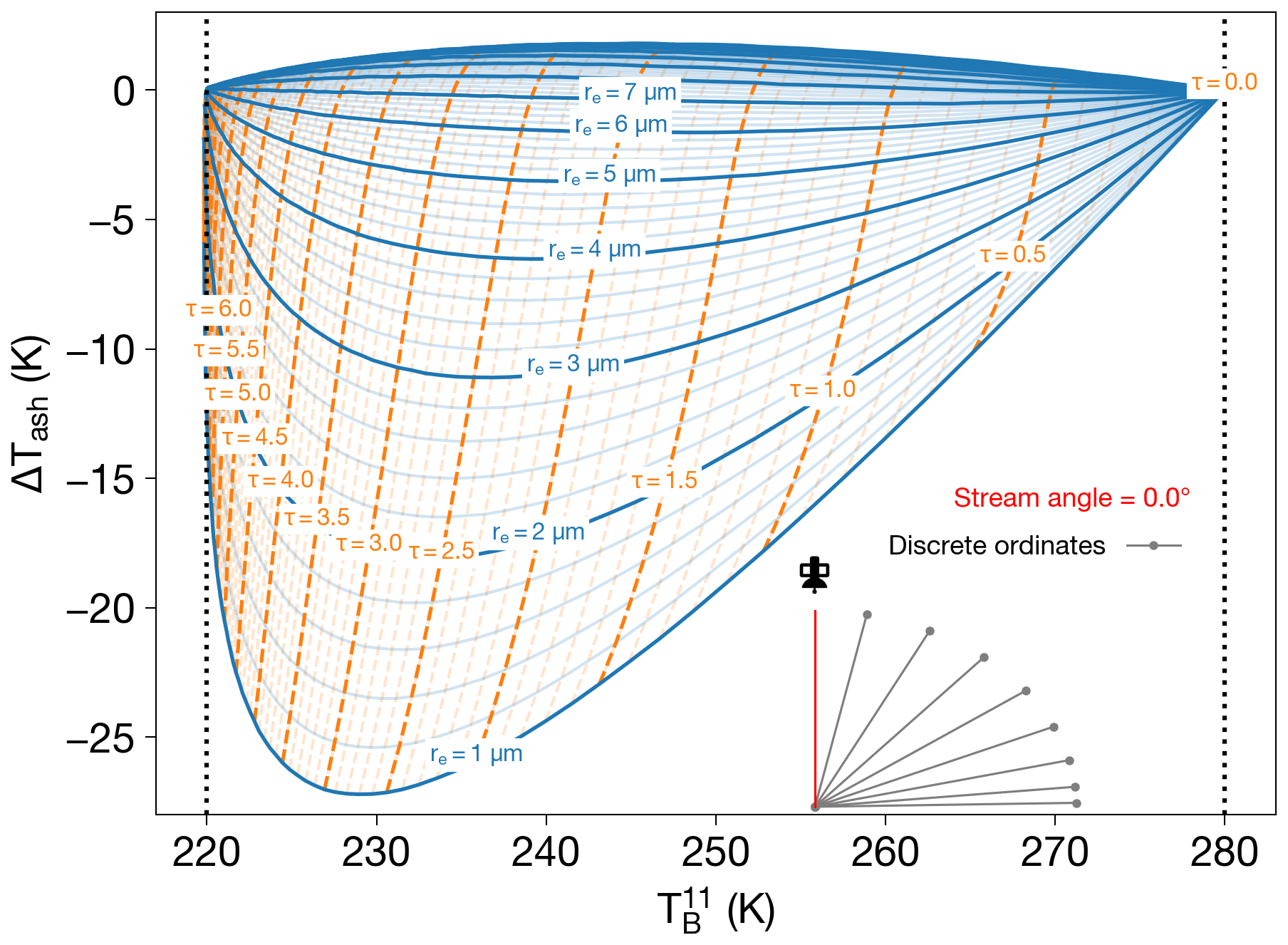
Figure A3 Graphical illustration of a volcanic ash look-up table for a surface temperature T_s=280 K and cloud-top temperature T_c=220 K. Dashed near-vertical lines indicate lines of constant optical depth, τ, and solid U-shaped curves indicate lines of constant effective radius, r_e.

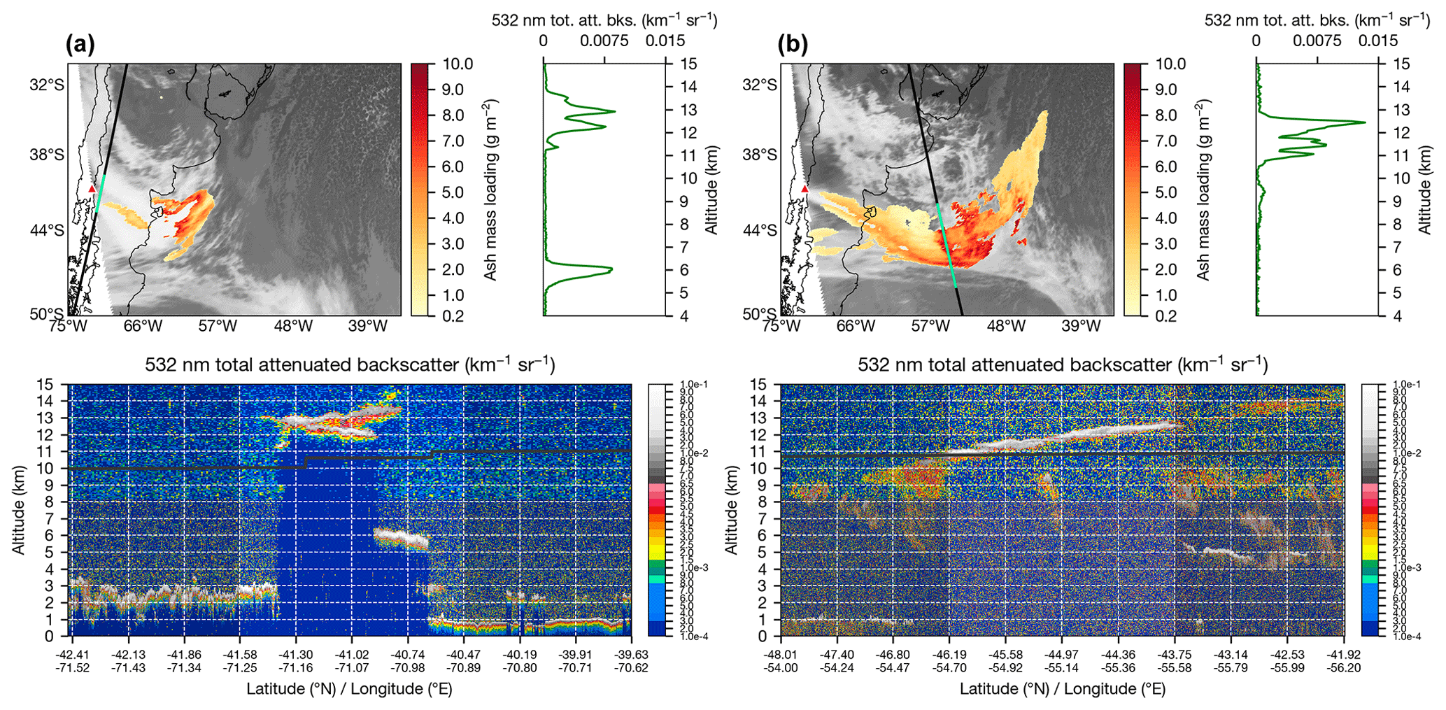
Figure A4 (a) SEVIRI ash mass loadings and CALIOP vertical profile of the Cordón Caulle ash plume on 5 June 2011 at 06:00 UTC. Top left panel: mass loading retrievals (yellow–orange–red colour scale) with brightness temperatures plotted underneath (red triangle indicates location of Cordón Caulle). Black line indicates CALIOP track and green highlight indicates full latitude–longitude range displayed in the bottom panel. Top right panel: 532 nm total attenuated backscatter profile averaged over the latitude–longitude range highlighted on bottom panel. Bottom panel: 532 nm total attenuated backscatter curtain (black line indicates the tropopause). Panel (b) is the same as (a) but for 5 June 2011 at 18:00 UTC.

To determine T_s directly from measurements, it is generally recommended to find a clear-air pixel near the volcanic cloud of interest (e.g. Wen and Rose, 1994) and can sometimes be determined by finding the maximum value of $T_{\mathrm{B}}^{\mathrm{11}}$ in the scene (Prata and Lynch, 2019). Obtaining an estimate for T_c from measurements, however, can be more difficult as the minimum value of $T_{\mathrm{B}}^{\mathrm{11}}$ may not correspond to the (semi-transparent) ash cloud of interest. Nevertheless, even if T_s and T_c can be reasonably estimated from measurements, it is often assumed that a single or mean value (and corresponding standard deviation) is representative of the entire ash cloud. Figure A1 shows that, in our case, the ash plume extends more than 60^∘ in longitude and 20^∘ in latitude, over land (including the Andes mountain range) and ocean, meaning that there is a considerable variation in cloud-top and surface temperature across ash-affected pixels. In addition, the meteorological setting within the considered spatial and temporal domains is complex (significant amounts of clouds), making estimates of T_s and T_c from measurements challenging for the Cordón Caulle case study. To account for variation in T_s and T_c across space and time, we use ERA5 reanalysis data Copernicus Climate Change Service (2017) to determine T_s and T_c at every ash-affected pixel over our study period of 5–10 June 2011 (in 1 h time steps).

To determine T_s from ERA5, we use the surface skin temperature (T_skin) and assume that the atmospheric transmittance (t_atm) has only a small effect on measured radiances at the top of the atmosphere for split-window channels (i.e. t_atm≈1). We also correct T_skin for variations in land surface emissivity using the University of Wisconsin global IR land surface emissivity database (Seemann et al., 2008). For ocean surfaces, we set the emissivity to 0.99, consistent with Western et al. (2015). Analysis comparing $T_{\mathrm{B}}^{\mathrm{11}}$ SEVIRI measurements against the emissivity-corrected T_skin for clear-sky pixels on 4 June 2011 indicates average differences of ∼ 2 K. To determine T_c from ERA5, we require an estimate of the volcanic cloud-top height. A fortuitous CALIPSO pass early on during the eruption on 5 June 2011 reveals that the Cordón Caulle ash cloud reached as high as 13–14 km above sea level (Fig. A4a), and later observations indicate heights from 10 to 13 km (Fig. A4b). For the retrievals presented here, we take T_c to be the ERA5 temperature at 13 km a.s.l. and make the simplifying assumption of constant height at all locations (and times) for every ash-affected pixel detected during 5–10 June 2011. The assumption of constant cloud-top height allows T_c to vary in time horizontally but less so vertically. However, FALL3D simulations indicate that the height of the Cordón Caulle ash cloud was relatively stable over the course of its dispersion in the atmosphere, and so we expect errors introduced by this assumption to be small. This was probably due to its injection into the stratosphere and its transport via the Southern Hemisphere jet stream (height variations from 11 to 15 km; Klüser et al., 2013; Vernier et al., 2013; Prata et al., 2017). For our study period from 5 to 10 June 2011, T_c ranged from 206 to 226 K, while T_s ranged from 230 to 304 K. We therefore performed radiative transfer calculations to construct unique LuTs, in steps of 2 K, for every possible combination of T_s and T_c within these ranges.

Appendix B: SO₂ retrieval

To retrieve total SO₂ column densities (in Dobson units; DU), we use the three-channel technique of Prata et al. (2003). This retrieval scheme exploits the strong SO₂ absorption feature near 7.3 µm and is only sensitive to upper-level SO₂ (>4 km) due to the absorption of lower-level water vapour at this wavelength. The three channels used to detect SO₂ using AHI measurements are centred around 6.9, 7.3 and 11.2 µm. To determine whether there is an SO₂ signal in the data, we first construct a synthetic 7.3 µm brightness temperature by interpolating from 6.9 to 11.2 µm in the radiance space and then converting to brightness temperature via the Planck function (Prata et al., 2003). Figure B1 illustrates how the interpolation procedure works in radiance space. The resulting “clear” brightness temperature ($T_{\mathrm{BC}}^{\mathrm{7.3}}$) is a good approximation of the measured value ($T_{\mathrm{B}}^{\mathrm{7.3}}$) in a SO₂-free atmosphere, so that one can identify SO₂ clouds by taking the difference between these two variables:

$$\begin{array}{}\text{(B1)}& \mathrm{\Delta }{T}_{{\mathrm{SO}}_{\mathrm{2}}}=T_{\mathrm{BC}}^{\mathrm{7.3}}-T_{\mathrm{B}}^{\mathrm{7.3}}.\end{array}$$

In theory, $\mathrm{\Delta }{T}_{{\mathrm{SO}}_{\mathrm{2}}}$ should be equal to zero under clear-sky conditions and increase with increasing SO₂ column density. However, in reality, high satellite zenith angles and variations in temperature and humidity can cause $\mathrm{\Delta }{T}_{{\mathrm{SO}}_{\mathrm{2}}}$ to be positive even under clear-sky conditions (Prata et al., 2003; Doutriaux-Boucher and Dubuisson, 2009). To remove false positives due to high satellite zenith angles and high water vapour burdens, we compute two SO₂-related BTDs (ΔT₆₉ and ΔT₈₆) and apply two successive temperature cut-off thresholds:

$$\begin{array}{}\text{(B2)}& \mathrm{\Delta }{T}_{\mathrm{69}}=T_{\mathrm{B}}^{\mathrm{6.9}}-T_{\mathrm{B}}^{\mathrm{7.3}}>T_{\mathrm{69}},\end{array}$$

where only those pixels with a ΔT₆₉ greater than a cut-off threshold of $T_{\mathrm{69}}=-\mathrm{2.5}$ K are flagged as potential SO₂. The second threshold takes advantage of the SO₂ absorption feature near 8.6 µm:

$$\begin{array}{}\text{(B3)}& \mathrm{\Delta }{T}_{\mathrm{86}}=T_{\mathrm{B}}^{\mathrm{11}}-T_{\mathrm{B}}^{\mathrm{8.6}}>T_{\mathrm{86}},\end{array}$$

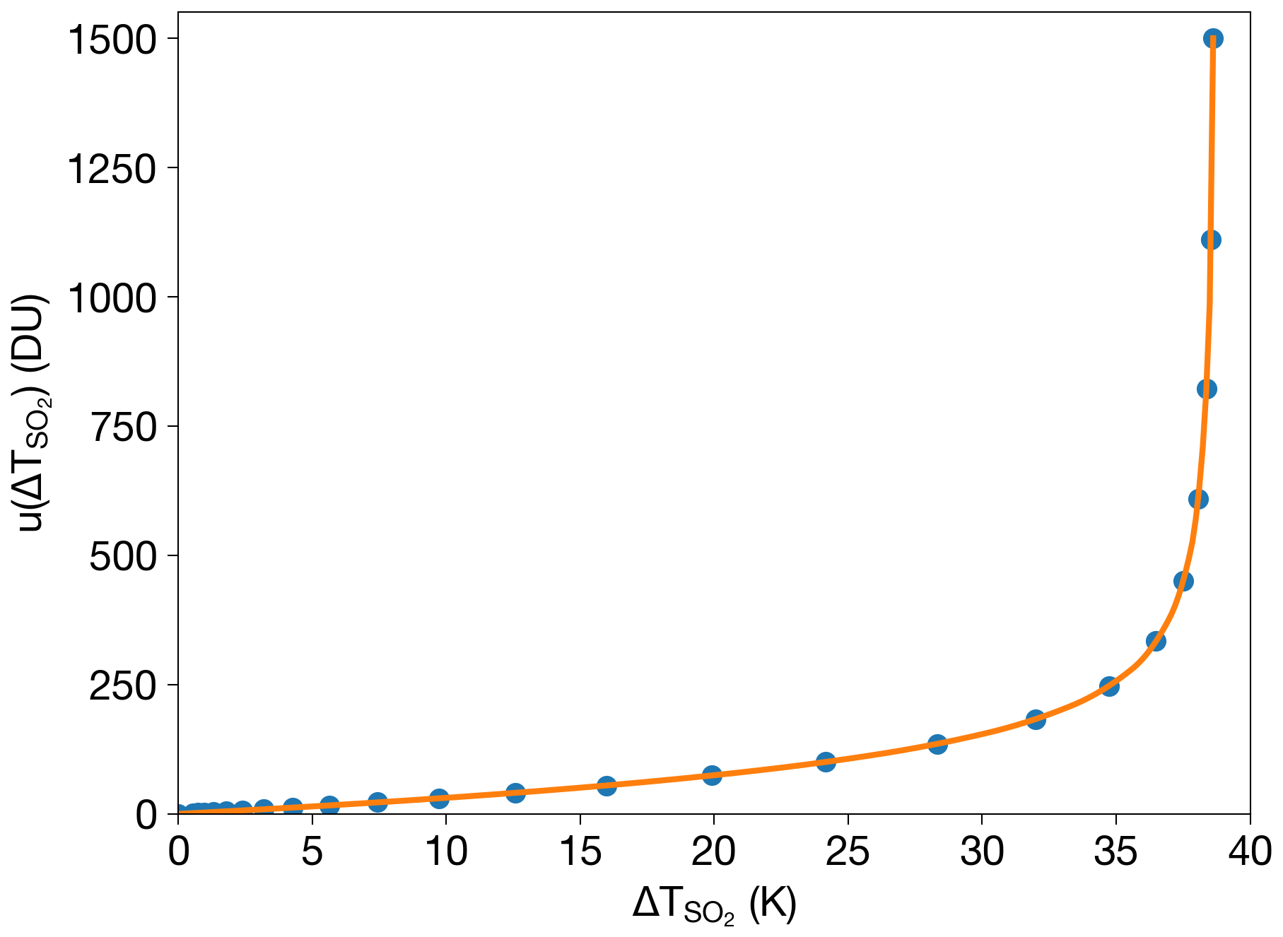
where only those pixels with a ΔT₈₆ greater than a cut-off threshold of T₈₆=3.5 K are flagged as potential SO₂. In addition, the presence of water and/or ice clouds and embedded volcanic ash can also affect the interpolation procedure used to construct $T_{\mathrm{BC}}^{\mathrm{7.3}}$. Figure B2a–c show, respectively, $T_{\mathrm{B}}^{\mathrm{7.3}}$, $T_{\mathrm{BC}}^{\mathrm{7.3}}$ and $\mathrm{\Delta }{T}_{{\mathrm{SO}}_{\mathrm{2}}}$ brightness temperatures for the SO₂-rich Raikoke cloud on 22 June 2019 at 21:00 UTC. Clearly, the interpolation procedure does a good job at removing the SO₂ signal from the measurements, resulting in excellent detection sensitivity for $\mathrm{\Delta }{T}_{{\mathrm{SO}}_{\mathrm{2}}}$. Comparison of Fig. B2d, e and f shows how the T₆₉ and T₈₆ thresholds are used to remove false alarms whilst preserving legitimate SO₂-affected pixels. Considering that $\mathrm{\Delta }{T}_{{\mathrm{SO}}_{\mathrm{2}}}$ calculated via Eq. (B1) is a function of the total column density of SO₂, we can retrieve the total column amount by constructing this function from offline radiative transfer calculations. For this purpose, we use the MODerate resolution atmospheric TRANsmission (MODTRAN) 6.0 code (Berk et al., 2014) to compute top-of-the-atmosphere (TOA) radiances at the 7.3 µm wavelength (Fig. A2b). All radiances determined from MODTRAN-6.0 were convolved using the AHI spectral response functions. These radiances are then converted to brightness temperatures to compute BTDs between an SO₂-free atmosphere and atmospheres with varying column densities of SO₂ at 7.3 µm (i.e. $\mathrm{\Delta }{T}_{{\mathrm{SO}}_{\mathrm{2}}}$). We are then able to generate a function representing the relationship between the SO₂ column density, $u\left(\mathrm{\Delta }{T}_{{\mathrm{SO}}_{\mathrm{2}}}\right)$ and $\mathrm{\Delta }{T}_{{\mathrm{SO}}_{\mathrm{2}}}$ by interpolating between the data points generated from the radiative transfer modelling (Fig. B4). In practice, we generate this function using a 1-D quadratic interpolation procedure implemented in the SciPy Python package (Virtanen et al., 2020). Atmospheric profiles of temperature, humidity and gases (H₂O, CO₂, O₃, N₂O, CO and CH₄) were taken from the US standard atmosphere. In varying the total SO₂ column densities (in DU), we must specify an SO₂ profile. We use CALIPSO total attenuated backscatter profiles collocated with Himawari-8 observations of $\mathrm{\Delta }{T}_{{\mathrm{SO}}_{\mathrm{2}}}$ to constrain the SO₂ profiles used in the radiative transfer calculations for the Raikoke case. Figure B3a shows a daytime CALIOP overpass intersecting SO₂ layers detected by Himawari-8 during the initial explosive phase of the Raikoke eruption. The vertical distribution of cloud–aerosol layers in the CALIOP observations reveals that the eastern part of the plume reached at least 12 km a.s.l. Later, CALIOP/AHI observations reveal complex stratospheric dynamics; two distinct components are apparent in the attenuated backscatter data with thin layers (1–2 km) present at 13–15 km in the northern part of the SO₂ cloud and ∼ 12 km in the southern part (Fig. B3b). Based on these initial observations, we constructed $u\left(\mathrm{\Delta }{T}_{{\mathrm{SO}}_{\mathrm{2}}}\right)$ using a uniform SO₂ distribution with a maximum cloud-top height of 13.5 km and thickness of 2.5 km (Fig. B4). The retrieval then proceeds by computing $\mathrm{\Delta }{T}_{{\mathrm{SO}}_{\mathrm{2}}}$ from AHI data and evaluating $u\left(\mathrm{\Delta }{T}_{{\mathrm{SO}}_{\mathrm{2}}}\right)$ for every SO₂-affected pixel.

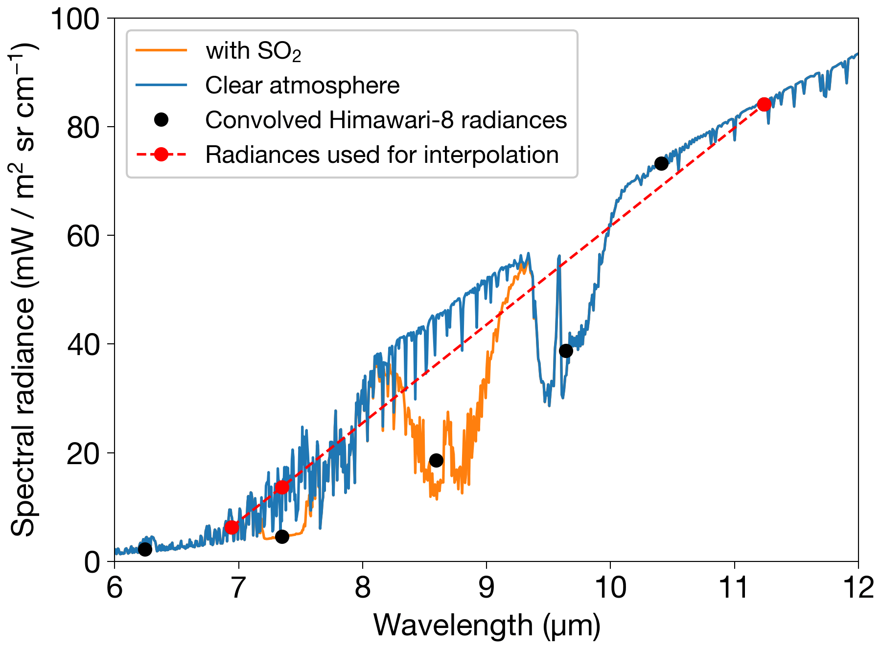
Figure B1 MODTRAN-6.0 simulations for atmospheres with and without SO₂ demonstrating how the interpolation procedure is used to estimate a clear-sky radiances from an atmosphere with SO₂. Convolved radiances were derived using the Himawari-8 spectral response functions.

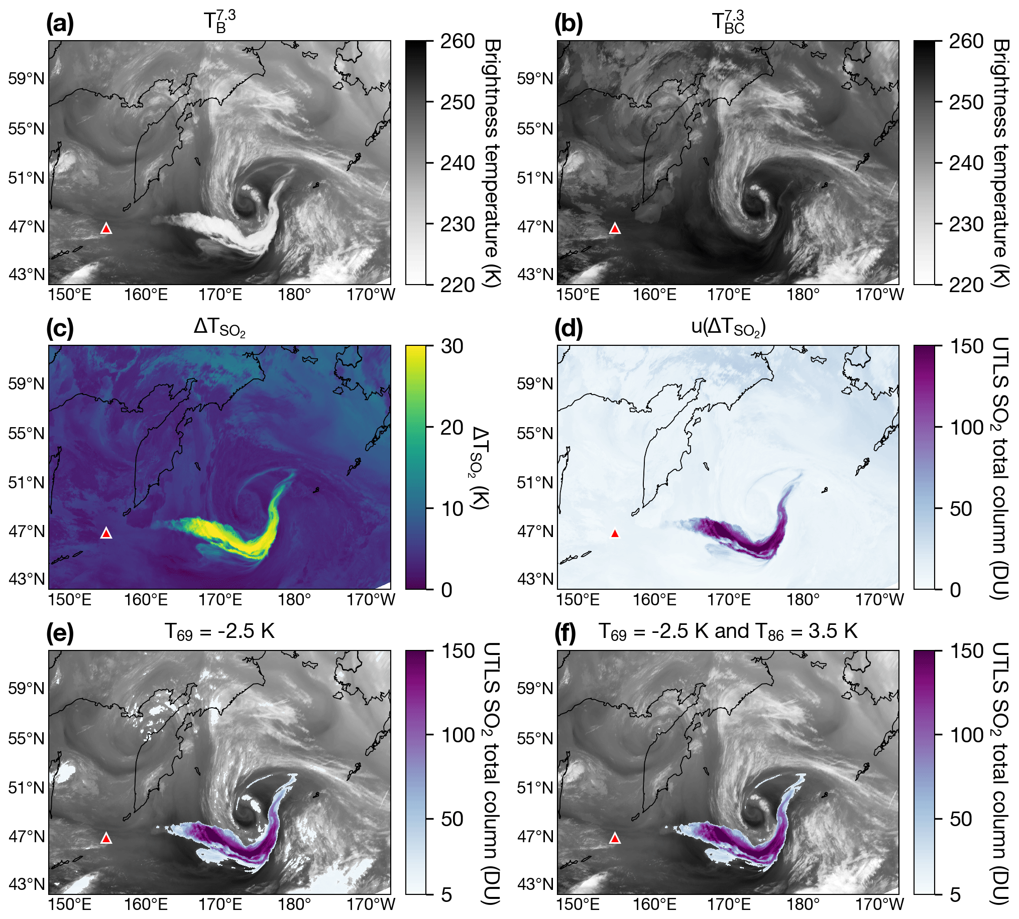
Figure B2 Volcanic SO₂ detection scheme applied to Himawari-8 observations of the Raikoke SO₂ cloud on 22 June 2019 at 21:00 UTC. The location of the Raikoke volcano is indicated by a red triangle on each map. (a) Himawari-8 brightness temperature at 7.3 µm ($T_{\mathrm{B}}^{\mathrm{7.3}}$). (b) Synthetic 7.3 µm brightness temperature ($T_{\mathrm{BC}}^{\mathrm{7.3}}$) determined from interpolation procedure (see Appendix B for details). (c) SO₂ BTD ($\mathrm{\Delta }{T}_{{\mathrm{SO}}_{\mathrm{2}}}=T_{\mathrm{B}}^{\mathrm{7.3}}-T_{\mathrm{BC}}^{\mathrm{7.3}}$). (d) SO₂ total column loading, u(ΔSO₂) (see Appendix B for details). (e) u(ΔSO₂) with $T_{\mathrm{69}}=-\mathrm{2.5}$ K and 5 DU thresholds. (f) u(ΔSO₂) with $T_{\mathrm{69}}=-\mathrm{2.5}$ K, T₈₆=3.5 K and 5 DU thresholds.

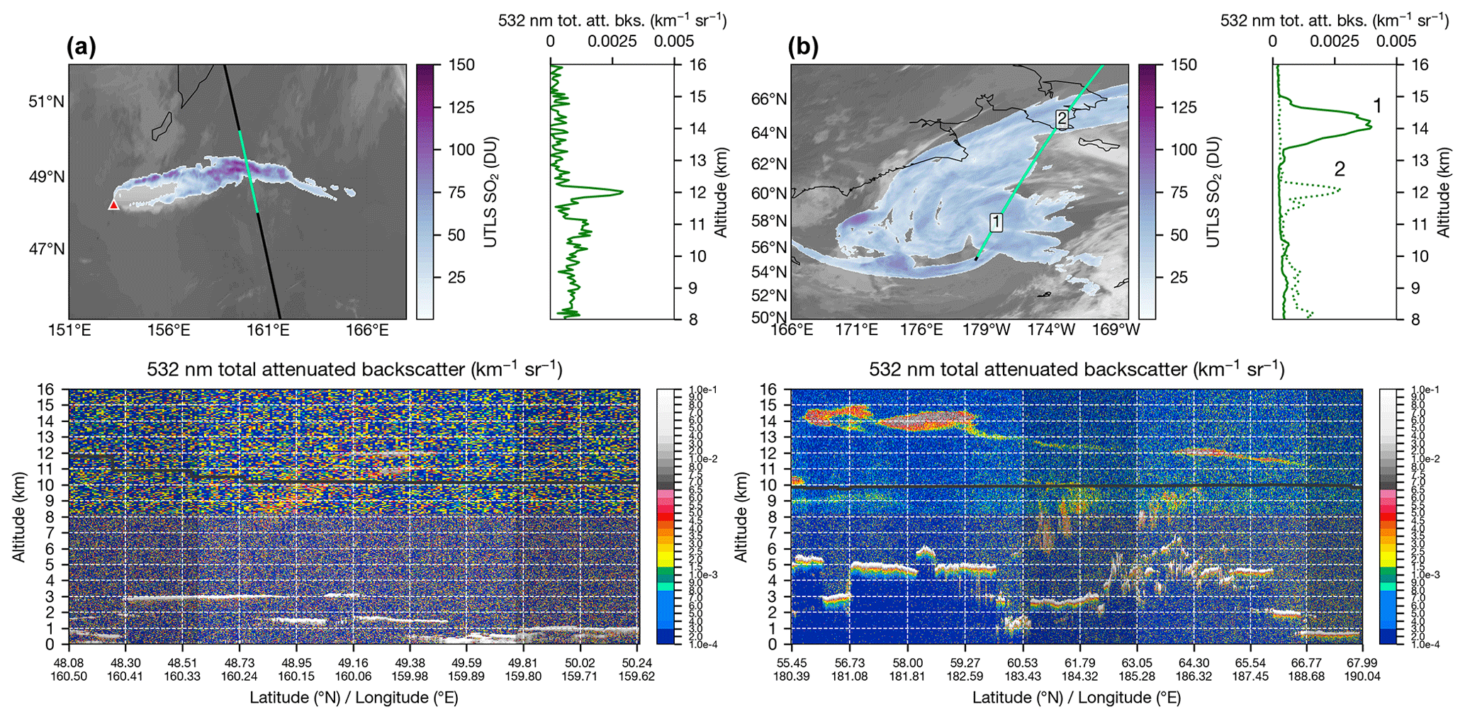
Figure B3 (a) AHI SO₂ UTLS total column burdens (DU) and CALIOP vertical profile of the Raikoke SO₂ plume on 22 June 2019 at 02:00 UTC. Top left panel: 7.3 µm SO₂ total column retrievals (white–purple–green–red colour scale) with 11 µm brightness temperatures plotted underneath (the red triangle indicates the location of Raikoke). The black line indicates CALIOP track and green highlight indicates full latitude–longitude range displayed in the bottom panel. Top right panel: 532 nm total attenuated backscatter profile averaged over the latitude–longitude range highlighted in the bottom panel. Bottom panel: 532 nm total attenuated backscatter curtain (the black line indicates the tropopause). Panel (b) is the same as (a) but for 25 June 2019 at 14:00 UTC.

Figure B4 MODTRAN-6.0 simulation results used to derive SO₂ total column density as a function of brightness temperature difference (see Eq. B1) for a uniform distribution with cloud-top height of 13.5 km and thickness of 2.5 km.