the Creative Commons Attribution 4.0 License.
the Creative Commons Attribution 4.0 License.
 | 17 Jun 2021
A model for urban biogenic CO2 fluxes: Solar-Induced Fluorescence for Modeling Urban biogenic Fluxes (SMUrF v1)
John C. Lin
Henrique F. Duarte
Vineet Yadav
Nicholas C. Parazoo
Tomohiro Oda
Eric A. Kort
When estimating fossil fuel carbon dioxide (FFCO2) emissions from observed CO2 concentrations, the accuracy can be hampered by biogenic carbon exchanges during the growing season, even for urban areas where strong fossil fuel emissions are found. While biogenic carbon fluxes have been studied extensively across natural vegetation types, biogenic carbon fluxes within an urban area have been challenging to quantify due to limited observations and differences between urban and rural regions. Here we developed a simple model representation, i.e., Solar-Induced Fluorescence (SIF) for Modeling Urban biogenic Fluxes (“SMUrF”), that estimates the gross primary production (GPP) and ecosystem respiration (Reco) over cities around the globe. Specifically, we leveraged space-based SIF, machine learning, eddy-covariance (EC) flux data, and ancillary remote-sensing-based products, and we developed algorithms to gap-fill fluxes for urban areas. Grid-level hourly mean net ecosystem exchange (NEE) fluxes are extracted from SMUrF and evaluated against (1) non-gap-filled measurements at 67 EC sites from FLUXNET during 2010–2014 (r>0.7 for most data-rich biomes), (2) independent observations at two urban vegetation and two crop EC sites over Indianapolis from August 2017 to December 2018 (r=0.75), and (3) an urban biospheric model based on fine-grained land cover classification in Los Angeles (r=0.83). Moreover, we compared SMUrF-based NEE with inventory-based FFCO2 emissions over 40 cities and addressed the urban–rural contrast in both the magnitude and timing of CO2 fluxes. To illustrate the application of SMUrF, we used it to interpret a few summertime satellite tracks over four cities and compared the urban–rural gradient in column CO2 (XCO2) anomalies due to NEE against XCO2 enhancements due to FFCO2 emissions. With rapid advances in space-based measurements and increased sampling of SIF and CO2 measurements over urban areas, SMUrF can be useful to inform the biogenic CO2 fluxes over highly vegetated regions during the growing season.
- Article
(18571 KB) - Full-text XML
-
Supplement
(13620 KB) - BibTeX
- EndNote


Climate change and urbanization are two major worldwide phenomena in recent decades. In close connection with both themes, cities have attracted increasing attention from both researchers and policy makers. Urban ecosystems are unique and complex given the wide variety of land use and land cover in cities, along with higher levels of atmospheric CO2 concentration, air temperature, and vapor pressure deficit than surrounding rural ecosystems (George et al., 2007). The consequences of climate change, such as severe heat, drought, and water shortage events, may be particularly exacerbated over (semi)arid and/or developing cities (Rosenzweig et al., 2018), resulting in possible population movement from increasingly hot and dry places to relatively cool and moist ones. Meanwhile, rapid urban expansion and population growth contribute to the rise in total anthropogenic CO2 emissions into the atmosphere and the urban heat island, which further influences plant phenology (Meng et al., 2020). Human activities have been continuously modifying the urban and natural vegetation and soil, e.g., expansion of agricultural lands at the cost of the natural landscape, leading to less reversible ecological and climatic impacts (Ellis and Ramankutty, 2008; Hutyra et al., 2014; Pataki et al., 2006). Hence, urban areas function as both biophysical and socioeconomic systems, and studying their carbon sources and sinks facilitates understanding cities' roles in the global carbon cycle.
To study the urban carbon pool and its exchange with the atmosphere, the top-down approach based on measured atmospheric CO2 concentrations is commonly used. McRae and Graedel (1979) noted over 4 decades ago that separation between anthropogenic and biogenic CO2 flux signals is needed to interpret urban CO2 observations. Biogenic CO2 fluxes are found to modify the surface CO2 and even atmospheric-column CO2 (XCO2) concentrations downwind (e.g., Lin et al., 2004; Turnbull et al., 2015; Hardiman et al., 2017; Sargent et al., 2018; Ye et al., 2020). For example, the seasonal variation in biogenic CO2 signals in Los Angeles was found to be one-third of the observed annual mean anthropogenic signal and further highlights the importance of urban irrigation (Miller et al., 2020). Over the Pearl River Delta in China, simulated biogenic contributions using 15 different models in the Multi-scale Synthesis and Terrestrial Model Intercomparison Project (MsTMIP; Huntzinger et al., 2013) lead to downwind XCO2 anomalies ranging from nearly zero up to 1 ppm depending on seasons and models, which reveals the non-neglectable biogenic influence on XCO2 as well as the large inter-model uncertainty (Ye et al., 2020). Thus, assessing the contributions from biogenic fluxes in observed signals is crucial for top-down estimates of urban emissions yet remains challenging, especially given limited urban flux observations across the globe. Although deciduous trees are found to be the dominant tree type in urban areas based on a meta-analysis of 328 global cities (J. Yang et al., 2015), a more accurate approximation of the vegetation coverages, types, and biological activities in cities is currently hard to obtain.
Existing approaches to separate biogenic and anthropogenic CO2 components involve the use of ancillary tracers and terrestrial biospheric models. For instance, since radiocarbon (14C) has decayed in fossil fuels, 14C serves as a tracer for the combustion of fossil fuel (FF) emissions (Miller et al., 2020; Turnbull et al., 2015). Carbonyl sulfide (COS) shares a similar seasonal variation as CO2 over land as a result of biospheric sinks (Kettle et al., 2002). However, measurements of 14C, COS, and CO2 fluxes are costly and lacking in most cities around the globe. Besides observations, many global terrestrial biospheric models provide insights to inform and constrain CO2 fluxes at continental to global scales (Huntzinger et al., 2013; Knorr and Heimann, 2001; Philip et al., 2019), but their relatively coarse resolution and simplifications of the urban biosphere limit their use for studying urban carbon cycles. Only a few biospheric models are designed for simulating urban biogenic fluxes. Research has revealed urban–rural differences in vegetation and soil properties, in part due to management strategies and environmental conditions, which complicate the flux quantification (Decina et al., 2016; Hardiman et al., 2017; Smith et al., 2019; Vasenev and Kuzyakov, 2018). Among these few models, the urban Vegetation Photosynthesis and Respiration Model (urbanVPRM; Hardiman et al., 2017) is an empirical model that incorporates the urban heat island effect and impervious surface area into its flux calculations and currently uses conventional greenness indices, e.g., the enhanced vegetation index (EVI).
Our work is primarily motivated by the relatively coarse spatial grid spacing and the simplifications of urban ecosystems in many models. We attempted to bridge the gap between coarse-scale global biospheric models and highly customized local models to offer a global solution to modeling biogenic CO2 fluxes within and around urban areas, which would provide insight into CO2 partitioning between fossil fuel and biogenic components.
Thanks to advances in spaceborne and ground-based measurements, solar-induced fluorescence (SIF) has been successfully retrieved from various satellite platforms and has proven to be an effective proxy for photosynthesis and thus modeling gross primary production (GPP) (Frankenberg et al., 2011; Guanter et al., 2014; Joiner et al., 2013; X. Yang et al., 2015). SIF tracks the unique seasonal and interannual variations in GPP across diverse plant functional types (PFTs) (Luus et al., 2017; Smith et al., 2018; Turner et al., 2020; Zuromski et al., 2018) and their responses to physiological stress (Magney et al., 2019). In an effort to improve long-term, high-resolution spatial mapping capabilities, several spatially continuous SIF products have been created using machine-learning (ML) techniques and light use efficiency modeling to combine satellite-retrieved SIF with ancillary vegetation data (Duveiller et al., 2020; Duveiller and Cescatti, 2016; Li and Xiao, 2019a; Turner et al., 2021; Zhang et al., 2018). Moreover, the empirical and PFT-specific linear correlations between GPP and SIF, derived from regressions of temporally aggregated (∼ monthly) eddy-covariance GPP (Frankenberg et al., 2011; Guanter et al., 2014; Magney et al., 2019; Sun et al., 2017; Turner et al., 2021; Zhang et al., 2018; Zuromski et al., 2018), have spurred the development of upscaled GPP estimates (Li and Xiao, 2019b; Yin et al., 2020). SIF information has also been incorporated into existing process-based biospheric models and data assimilation systems (MacBean et al., 2018; Van Der Tol et al., 2009). Within the context of the urban biosphere, SIF retrieved from space has been shown to reveal the urban–rural gradient in photosynthetic phenology (Wang et al., 2019). Given all these advantages, SIF would potentially benefit GPP estimates and CO2 flux partitioning over cities.
Ecosystem respiration (Reco), the other component of net ecosystem exchange (NEE), is defined as the sum of the autotrophic (RA) and heterotrophic (RH) components. In terms of modeling urban Reco, urbanVPRM follows the conventional approach of VPRM (Mahadevan et al., 2008) to estimate an initial air-temperature-scaled (Tair-scaled) Reco and splits Reco into equal components (RA and RH) that will be further modified by considering impervious fractions and urban heat island effects (Hardiman et al., 2017). However, the exact partitioning of Reco between RA and RH as well as the separation between aboveground and belowground respiration can be challenging and highly uncertain, as acknowledged in Hardiman et al. (2017). The initial Reco that urbanVPRM modified may be an overly simplistic function of ambient air temperature. After all, the complexity of biological and nonbiological processes of Reco and the lack of a mechanistic understanding of how biotic and abiotic factors affect Reco render mechanistic modeling of Reco challenging. Given the complexity in modeling Reco, we will turn instead to ML techniques that have been increasingly applied in many disciplines to help answer complicated, entangled problems by extracting patterns from data streams for predictions and generalizations. Reichstein et al. (2019) provided a comprehensive review of the many applications of ML techniques in solving geoscience and remote sensing problems and identified challenges in successfully adopting ML approaches – e.g., interpretability, integration with physical understanding and modeling, and the ability to cope with model–data uncertainties. In the context of ecosystem modeling, an artificial neural network (NN) has been utilized to generate SIF beyond satellite soundings (Li and Xiao, 2019a; Zhang et al., 2018), harmonize multiple SIF satellite instruments (Wen et al., 2020), map carbon and energy fluxes (Tramontana et al., 2016), and reveal and predict the trend in global soil respiration (Zhao et al., 2017).
In this paper, we present a model representation of GPP, Reco, and NEE fluxes targeting urban areas around the globe, the Solar-Induced Fluorescence (SIF) for Modeling Urban biogenic Fluxes (“SMUrF”), by taking advantage of SIF and the NN technique. Our main objectives include (1) examining the biogenic and anthropogenic CO2 fluxes and their temporal variations over urban and surrounding rural areas and (2) demonstrating one application of SMUrF to help interpret satellite CO2 observations by revealing the urban–rural gradient in biogenic CO2 fluxes along satellite swaths of the Orbiting Carbon Observatory 2 (OCO-2; Crisp et al., 2012).
SMUrF incorporates SIF as an indicator of photosynthesis, along with possible drivers for Reco (i.e., air and soil temperatures and SIF-driven GPP), and performs hourly downscaling using reanalysis-based temperature and radiation fields (Fig. 1). We accounted for variations in biome types and Reco at 500 m before aggregating fluxes to the final grid spacing of 0.05∘. Gridded uncertainties of daily mean fluxes are quantified by assigning a biome-specific coefficient of variation (CV) from model–data comparisons (Sect. 2.5). To gain insight into the column CO2 anomalies caused by anthropogenic and biogenic fluxes, we further adopted an atmospheric transport model to link fluxes and concentrations (Sect. 2.6). Before introducing the steps for estimating individual flux components, we first go through the main input datasets (Sect. 2.1).
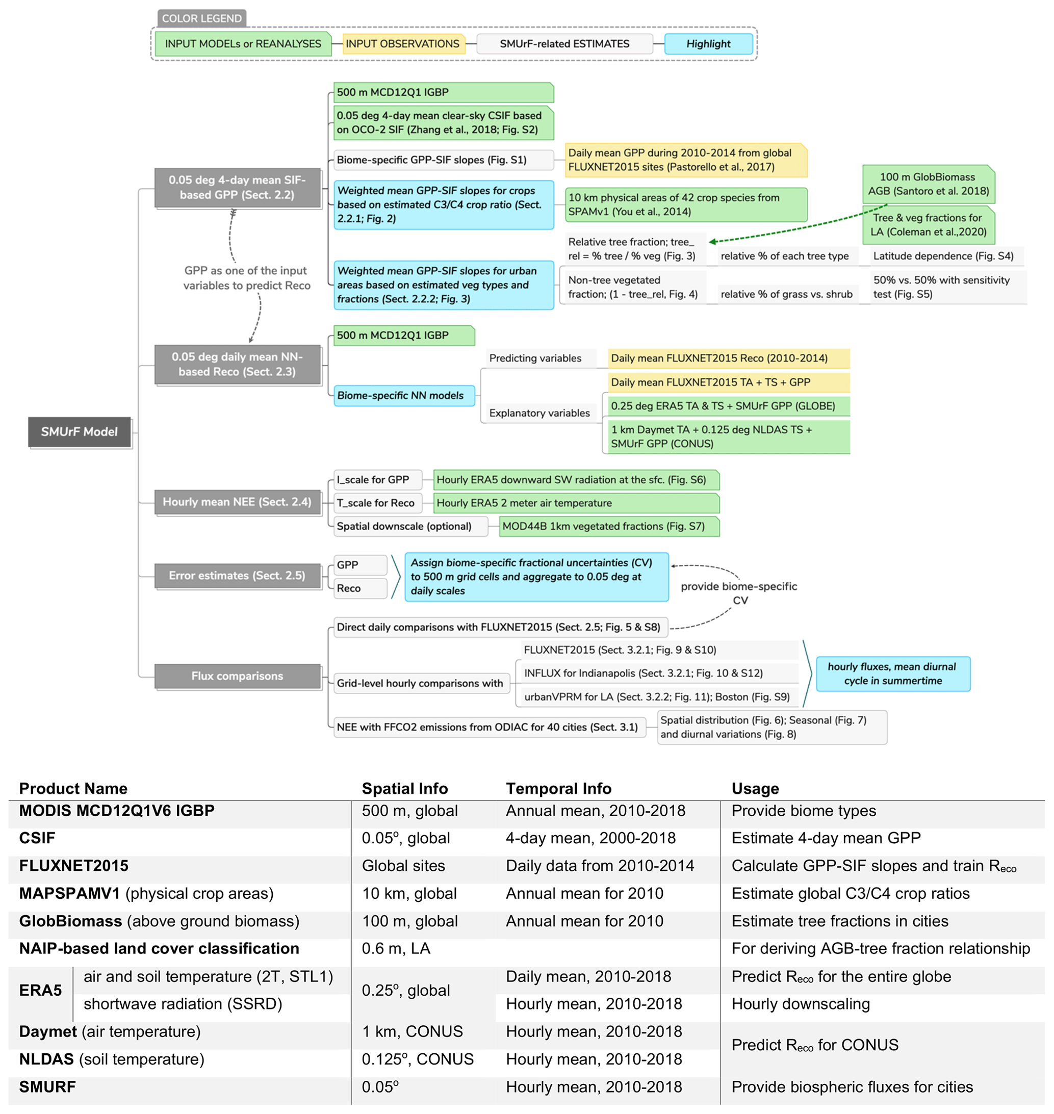
Figure 1A demonstration of SMUrF (flowchart) and a description of input data products and observations (summarized in the table). The temporal coverage in the table indicates the years used in this study.
2.1 Input datasets
Similar to many biospheric models, SMUrF estimates gridded GPP, Reco, and NEE (= Reco – GPP) fluxes based on land cover types. Main required data streams are summarized in Fig. 1, including (1) the 500 m MODIS-based land cover classification, (2) the 0.05∘ spatiotemporally contiguous SIF (CSIF) product, (3) 100 m aboveground biomass (AGB) from GlobBiomass, (4) eddy-covariance (EC) flux measurements across continents, and (5) gridded products of air and soil temperatures.
2.1.1 Land cover classification
Land cover classifications with more sophisticated algorithms in urban areas (e.g., NLCD 2016) are often available for limited regions. Thus, we adopted the land cover types defined by the International Geosphere–Biosphere Programme (IGBP) from MCD12Q1 v006 (Friedl and Sulla-Menashe, 2019) to inform biome types over global land. The 12 biomes include croplands (CRO), closed and open shrublands (CSHR, OSHR), five types of forest (deciduous broadleaf – DBF, deciduous needleleaf – DNF, evergreen broadleaf – EBF, evergreen needleleaf – ENF, mixed forests – MF), grasslands (GRA), savannas (SAV), woody savannas (WSAV), and permanent wetlands (WET). Since MCD12Q1 simply treats the entire urban area as one category (URB), we developed an algorithm to approximate the vegetation types and fractions in cities (Sect. 2.2.2).
2.1.2 Data for GPP estimates
We used the spatiotemporally contiguous SIF (CSIF; Zhang et al., 2018) product and GPP fluxes from FLUXNET2015 (Pastorello et al., 2017) to calculate biome-specific GPP–CSIF slopes (α, Fig. S1 in the Supplement). A total of 98 global EC tower sites with screened data points (quality flag < 3) from 2010 to 2014 are chosen to represent various biomes. CSIF offers global 4 d mean SIF at a grid spacing of 0.05∘ during 2000–2018 using the NN approach (Zhang et al., 2018). The NN model in CSIF is constructed based upon OCO-2 SIF and four broadband reflectances from MCD43C4 V006 under clear-sky conditions, and it is used for mapping SIF beyond sounding locations. CSIF agrees well with SIF retrievals from OCO-2 and GOME-2, considering the inevitable spatial mismatch between CSIF (0.05∘) and the direct sounding-level SIF measurements (OCO-2's footprint of ∼ 1 km × 2 km). The two largest biases of CSIF with respect to OCO-2 SIF arise from croplands (−12.72 %) and urban areas (−14.59 %), caused by the saturation effect in broadband reflectances and built-up contamination in the reflectance signal, respectively (Zhang et al., 2018). To compensate for the potential bias of urban CSIF, we scale up the GPP–SIF slope for urban areas (details in Sect. 2.2.2).
In addition, the clear-sky instantaneous CSIF is compared to TROPOMI-based downscaled SIF for summer 2018 (Turner et al., 2021) and vegetated fractions inferred from the WUDAPT product (Appendix A). Despite some discrepancies over a few regions, these comparisons confirmed CSIF's performance and capability in revealing the urban–rural gradient in biogenic activities (Figs. S2–S3).
2.1.3 Data for approximation of urban vegetation globally
To assign trees and grass within the MODIS-based urban domain, several steps are carried out to approximate the relative fractions of (1) tree versus non-tree, (2) individual tree types, and (3) grassland versus shrubland (details in Sect. 2.2.2). Relative tree fractions (i.e., ratio of tree fractions to total vegetated fractions) can be obtained from two data sources: a 0.6 m urban land cover product (Coleman et al. 2020) based on the National Agriculture Imagery Program (NAIP) and a 250 m vegetation continuous field (VCF) from MOD44B (Dimiceli et al., 2015). Both products offer estimated tree and vegetated fractions. The former one is produced only over Los Angeles via random forest algorithms that trained on Sentinel-2 (∼ 5 m) and NAIP (∼ 0.6 m) optical imagery (Coleman et al., 2020), and it possesses much higher tree fractions than MODIS VCF (see comparisons in Sect. 2.2.2). Thus, we decided not to utilize MODIS VCF for indicating urban vegetation in this work, only for comparing tree fractions from Coleman et al. (2020).
To approximate relative tree fractions (ftree) in cities, we treat the gridded AGB at 100 m from GlobBiomass (Santoro et al., 2018) as the spatial proxy (see the methodology explanation in Sect. 2.2.2). GlobBiomass deployed a complex retrieval algorithm system that involves a series of retrieval algorithms using radar backscatter and several other data types such as laser measurements from ICESAT (Schutz et al., 2005), tree and land cover data (e.g., from Landsat), and collections of reanalyses and models. AGB and its grid-level uncertainty [t ha−1] by definition describe the “oven-dry weight of the woody parts (stem, bark, branches, and twigs) of all living trees excluding stump and roots” (Santoro et al., 2018). GlobBiomass AGB has demonstrated good agreement with independent data products for different continents (Santoro et al., 2018).
2.1.4 Reanalyses for Reco estimates
In an effort to train and predict Reco via neural network models, we chose GPP as well as air and soil temperatures (Tair and Tsoil) as explanatory variables (details in Sect. 2.3). Modeled Tair and Tsoil are taken from the ECMWF ReAnalysis-5 (ERA5, 0.25∘; Copernicus Climate Change Service Information, 2017) for the entire globe or from Daymet (1 km; Thornton et al., 2016) and the North American Land Data Assimilation System (NLDAS; 0.125∘; Xia et al., 2012) as alternative inputs for CONUS runs (Fig. 1). It is worth pointing out that different models and reanalyses provide Tair at 2 m above the ground but Tsoil at different soil depths. For instance, four soil depths from NLDAS are 10, 30, 60, and 100 cm below the ground, whereas ERA5 simulates mean Tsoil over four vertical layers, i.e., 0–7, 7–28, 28–100, and 100–289 cm. Measured soil depths from FLUXNET are even more complicated and vary among sites, with the most common shallowest soil depth at ∼ 2 cm below the ground. To reconcile differences in soil depths, we chose measured Tsoil from the shallowest layer in both the model and observational datasets to separately build NN models (Sect. 2.3).
2.1.5 Data for flux comparisons
We further carried out flux comparisons against two independent sets of eddy-covariance data, i.e., FLUXNET2015 and the Indianapolis Flux Experiment (INFLUX; Davis et al., 2017; K. Wu, 2020), and one alternative urban biospheric model (urbanVPRM) over Los Angeles in Sect. 3.2. Only non-gap-filled measured NEE fluxes from FLUXNET2015 (with a quality flag of 0) are used for validation. Since NEE fluxes measured from INFLUX have not been gap-filled, we only chose the hours from SMUrF when valid INFLUX data are available.
The INFLUX project includes EC flux measurements that accompany the tower- and aircraft-based greenhouse gas (GHG) mole fraction measurements. These sites have been periodically moved to sample different components of the urban landscape. For the period from 10 August 2017 to 7 June 2019, these flux towers were deployed at two urban vegetation sites (no. 1 and no. 4) and two agricultural sites (no. 2 and no. 3). Two urban vegetation (turf grass) sites were located in a cemetery area (site no. 1) and on a golf course (site no. 4). Because CSIF is not available beyond 2018 at the time of writing, we cannot yet extend the flux comparison into 2019. Fluxes from INFLUX sites were computed using EddyPro software (LI-COR Biosciences, 2012) and post-processed to filter out data when (a) the LI-COR gas analyzer signal strength was low and (b) during periods of weak turbulence (K. Wu, 2020). It is worth noting that INFLUX data provide valuable independent evaluations as flux sites with an urban imprint are lacking from FLUXNET2015, and observed fluxes from INFLUX sites were not used when calibrating parameters in SMUrF.
The urbanVPRM, applied over Los Angeles, estimates GPP from a light use efficiency modeling perspective driven by reanalysis-based photosynthetically active radiation (PAR) as well as the satellite-derived EVI and land surface water index (LSWI) for phenology and water availability. It estimates Reco via an air temperature function with extra modifications to air temperature due to the urban heat island effect and impervious surface area. The urbanVPRM-based fluxes rely on the 60 cm NAIP-based land cover classification in Los Angeles (Coleman et al., 2020; Sect. 2.1.3). Due to differences in grid spacing between models, fluxes from urbanVPRM are aggregated and re-projected from 30 m to 0.05∘ to match SMUrF for the purposes of comparison.
2.2 GPP estimates
We used 4 d mean clear-sky SIF from CSIF and 4 d mean observed GPP fluxes from 98 global eddy-covariance (EC) towers from FLUXNET2015 to derive biome-specific GPP–SIF slopes (α, Fig. S1) with special treatments to α over croplands and urban areas, as described in the following subsections. While nonlinear relationships between SIF and GPP at leaf and canopy level have been observed (Helm et al., 2020; Magney et al., 2017; Maguire et al., 2020; Marrs et al., 2020; Verma et al., 2017), GPP is observed to be linearly related to SIF at increasing temporal and spatial (ecosystem and regional) scales (Frankenberg et al., 2011; Sun et al., 2017) as leaf-level differences in composition, light exposure, stress, and stress response mix out (Magney et al., 2020). Considering uncertainty in CSIF and flux-tower-partitioned GPP as well as the noise in the GPP–SIF relationship across global flux sites (Fig. S1), we adopted linear fits instead of nonlinear fits between GPP and CSIF. Errors due to departure from linearity will be implicitly included in GPP uncertainties calculated from model–tower validations (Sect. 2.5). The calculated α values are in proximity to those reported in Zhang et al. (2018) from 40 towers and are assigned to each 500 m grid cell according to the corresponding biome type.
2.2.1 C3 C4 partitioning of croplands
GPP–SIF relationships differ between C4 and C3 crops at the canopy scale, since GPP for C3 crops may saturate at high PAR levels. Different statistical fits between observed GPP and SIF are suggested for C3 versus C4 crops (He et al., 2020). Despite the focus of SMUrF on urban areas, we still attempted to differentiate C4 from C3 crops and estimate two different α values from EC sites dominated by C3 or C4 crops. Specifically, the Spatial Production Allocation Model (SPAM 2010V1.1; You et al., 2014) is used for areal estimates of 42 crop species, among which the following are identified as C4 crops: maize, pearl and small millet, sorghum, and sugarcane. As a result, we produced maps of C3 : C4 ratios at a grid spacing of 10 km for the entire world (Fig. 2a, b). Four of the selected 13 cropland EC FLUXNET sites fall within grid cells with a high C4 ratio of > 50 %; the remaining sites fall into grid cells with C4 ratios of < 10 %. We thereby arrive at of ∼ 35.6 [µmol m−2 smW m−2 nm−1 sr−1] from sites with a high C4 ratio and of ∼ 19.7 [µmol m−2 s−1] : [mW m−2 nm−1 sr−1] from the other nine cropland sites. Eventually, we calculated the weighted mean α according to the C3 : C4 ratio map and identified tropical regions, the midwestern US, northeastern China, and spots in India and southern Africa as regions with higher α and C4 crop ratios (Fig. 2c). Note that these weighted mean α values will only be activated over MODIS-based croplands.

Figure 2Spatial distribution of the estimated C3 : C4 ratio [%] (a–b) using physical areas of 42 crop species from MapSPAMv1 and weighted mean GPP–CSIF slopes [()(mW m−2 nm−1 sr−1)] for croplands (c).
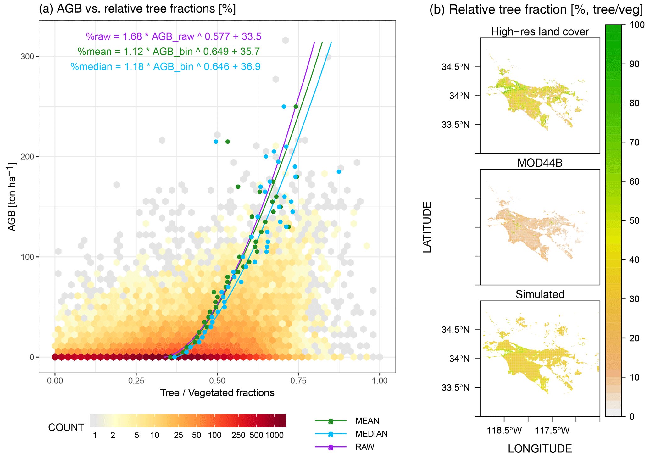
Figure 3(a) Power-law relationships fitted between the aboveground biomass (AGB) and raw relative tree fractions (purple line) as well as fits using binned AGB and mean or median relative tree fractions per AGB bin (green or blue lines). The statistical fit in purple is chosen to predict relative tree fractions within cities. (b) Spatial distributions of calculated relative tree fractions (%) from a high-resolution NAIP-based land cover classification product (Coleman et al., 2020) (top panel), vegetation continuous fields from the MOD44B v6 product (middle panel), and our approximation (bottom panel) using AGB and the statistical fit illustrated in panel (a).
2.2.2 Modification to urban vegetation
We next turn to the estimate of α over the MODIS-based “urban” category shown in the following three steps (Fig. 1).
-
Estimate the relative tree fraction (ftree= tree / vegetation). A power-law relationship (Fig. 3a) between AGB bins and relative tree fractions obtained from the NAIP-based land cover classification (top panel in Fig. 3b) is used to predict ftree (bottom panel in Fig. 3b). Although the AGB binning procedure may not fully recreate the variations in ftree, especially for grid cells with zero AGB (dark red hexagons in Fig. 3a), the predicted ftree using AGB is tied to a smaller bias of +2.3 % than ftree using MOD44B (−23.5 %) when the high-resolution NAIP-based land cover product is compared (Fig. 3b).
-
Estimate relative fractions of five tree types, grass, and shrubs based on climatology. Due to the lack of global data on urban biome types, the relative non-tree vegetated fraction () is simply split into half grass and half shrub (second row in Fig. 4). The relative tree fractions are divided into five possible tree types (i.e., DBF, DNF, EBF, ENF, MF). The share of each tree type in cities is approximated as a function of latitude based on the climatology of land cover types (Fig. S4a), e.g., high fractions of ENF over high latitudes, EBF over tropical lands, and DBF plus MF over the midlatitudes (Fig. S4b).
-
Calculate weighted mean α. The α values for urban areas are weighted mean values calculated from biome-specific α values and their corresponding fractions approximated in step 2. To account for the potential negative bias of ∼ 14.5 % in CSIF over cities (Zhang et al., 2018), we scaled up urban α by 1.145.
In the end, α values at 500 m over urban and natural lands (third row in Fig. 4) are aggregated to 0.05∘ and multiplied by CSIF to arrive at GPP at 0.05∘. The exact partitioning between grass and shrub in step (2) plays a minor role in the final GPP flux at 0.05∘ (Fig. S5). It is worth clarifying that we implicitly assumed that vegetation “exists” over urban grid cells and only solved for the relative tree versus grass fractions as illustrated in steps (1) and (2), as information on vegetated and impervious fractions has been embedded in the CSIF product. Additional information about vegetated and impervious fractions was not necessary in the calculation of α for every 500 m urban grid (see Appendix A for a further explanation).

Figure 4Estimated relative deciduous broadleaf forest (DBF, first row) and non-tree fractions (fnon-tree, second row) at 500 m as well as GPP–SIF slopes after urban gap filling (third row) for Los Angeles (a), Chicago (b), and Boston (c).
2.3 Reco estimates
Three explanatory variables – Tair, Tsoil, and GPP – are chosen to train against the observed daily mean Reco from FLUXNET. To account for mismatches in reported soil depths (introduced in Sect. 2.1.4), we built separate sets of NN models using (1) direct temperatures and GPP observations from EC towers, (2) ERA5-based temperatures and SIF-based GPP, or (3) Daymet and NLDAS-based temperatures and SIF-based GPP (only for the US as alternative runs). SIF-based GPP is ingested in order to pass SIF information on to Reco estimation. Data points from a few EC sites with relatively large uncertainties in modeled GPP were excluded before the training of NN models to prevent error propagation into Reco (Appendix B).
For each set of NN models, we manually split data points based on their biome types and obtain 12 separate NN models. Data points from open and closed shrublands are combined due to the extremely low numbers of EC sites around the globe. To be consistent with the C3 : C4 crop partition for GPP estimates (Sect. 2.2.1), we obtained two separate NN models for C3 and C4 crops and calculated the weighted mean Reco based on the derived C3 : C4 ratios. 80 % and 20 % of the data points per biome are used for training and testing, respectively. Models with two hidden layers are constructed with 32 and 16 neurons chosen for the first and second layer. We computed Reco at 500 m by applying biome-specific models and aggregated those Reco to 0.05∘. We also tested two alternative ways to train Reco based on (1) all data points without differentiating their land cover types and (2) additional categorical variables from biomes and the month and season of the year. Please refer to Appendix B for sensitivity tests and technical details about data preparation and cross-validation of neural networks.
2.4 NEE estimates
We obtained hourly surface downward shortwave radiation (SWrad) and air temperature (Tair) from the ERA5 reanalysis to calculate the hourly scaling factors for GPP and Reco. Tair and SWrad are initially provided at a grid spacing of 0.25∘ and then bilinearly interpolated to 0.05∘. To estimate the hourly radiation scaling factors Iscale for GPP, we normalized the hourly SWrad by the 4 d mean SWrad with the same time window of the 4 d mean GPP. Regarding the calculation of hourly temperature scaling factors Tscale for Reco, a temperature sensitivity function (SR1 h) has been modified from prior studies (Fisher et al., 2016; Olsen and Randerson, 2004):
where Q10 is a unitless temperature sensitivity parameter that could vary across biomes, and Tair is in degrees Celsius (∘C). Because the hourly downscaling procedure is performed on GPP and Reco fluxes at 0.05∘ and no single biome is tied to each 0.05∘ grid cell, we adopt a typical Q10 value of 1.5 according to previous studies (Fisher et al., 2016) despite possible biome-dependent variations in Q10. SR1 h is then normalized by its daily mean value to obtain Tscale. Finally, Tscale and Iscale are used to temporally downscale the daily mean Reco and 4 d mean GPP, i.e., and .
Examples of Iscale and Tscale over the western US on 2 July 2018 are displayed in Fig. S6bc. As a sanity check for the ERA-based SWrad, a higher-resolution product is utilized, from which SWrad and PAR were estimated based on Earth Polychromatic Imaging Camera (EPIC, on board the Deep Space Climate Observatory – DSCOVR) data and random forest algorithms (Hao et al., 2020a, b). The EPIC-based radiation data are available globally at 10 km from June 2015 to June 2019 and have been validated against in situ observations from the Baseline Surface Radiation Network and Surface Radiation Budget Network. Hourly Iscale values using ERA5-based SWrad and EPIC-based SWrad or PAR generally agree well regarding the diurnal cycles, despite small discrepancies in peak radiation and Iscale values during noon hours (Fig. S6de).
2.5 Uncertainty quantification and direct flux validation
Error quantification is important for characterizing the precision and accuracy of modeled fluxes. Previous studies have carried out comprehensive uncertainty estimates towards their reported biogenic flux estimates (Dietze et al., 2011; Hilton et al., 2014; Lin et al., 2011; Xiao et al., 2014). Here we estimated errors in modeled GPP and Reco based on FLUXNET observations.
We extrapolated the biome type, 4 d mean SIF, and daily mean Tair and Tsoil from their original gridded fields to each flux tower location and directly computed the modeled GPP and Reco using α values and NN models. Comparisons between these direct computations and screened observations from FLUXNET2015 yield biome-specific root mean square errors (RMSEs), mean biases, and CVs. The uncertainties in assuming a linear GPP–SIF relationship were not explicitly quantified but incorporated within these error statistics on top of other error sources such as inter-site variations. Eventually, biome-specific CVs are assigned to each 500 m grid and aggregated to 0.05∘ assuming statistical independence. For visualization purposes, we collected model–data pairs regardless of their biome types as density plots in Fig. 5.
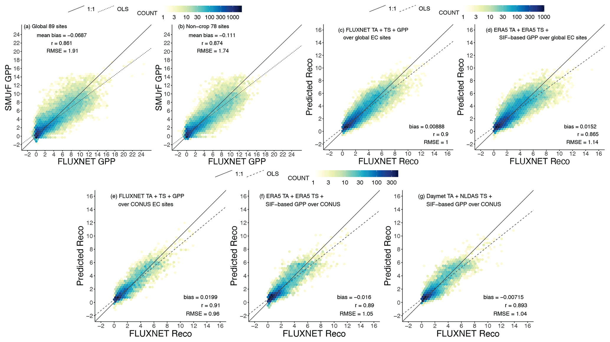
Figure 5Comparisons between directly computed fluxes from SMUrF and observed fluxes from FLUXNET during 2010–2014 as density plots with 50 bins. All fluxes have units of µmol m−2 s−1. (a–b) 4 d mean observed GPP and directly computed SIF-based GPP at 89 global EC sites (a) and 78 non-crop sites (b). (c–d) An evaluation of the daily mean observed Reco and predicted Reco in the testing set (i.e., 20 % of all data) using observed GPP from FLUXNET (c) or Tair+Tsoil from ERA5 and SIF-based GPP (d) for 89 global EC sites. (e–g) Similar to panels (c)–(d), but the model–data Reco comparison only for US EC sites and modeled Reco is calculated using Daymet Tair, NLDAS Tsoil, and SIF-based GPP (g). Although GPP and Reco were trained and predicted separately per biome, model–data pairs from all biomes are collected for visualization purposes. For each panel, numbers of data points in each of the 50 bins are displayed in log10 scales as yellow–blue colors, and error statistics including the mean bias, correlation coefficient, and RMSE are printed. The 1:1 and ordinary-least-square-based (OLS-based) regression lines are displayed as solid and dashed lines. RMSEs derived from these direct validations were further used for assigning uncertainties at the 500 m grid cell (Sect. 2.5).
Directly computed 4 d mean GPP values at most towers match observations well regarding their magnitude and seasonality. Modeled GPP shows underestimations against irrigated maize sites in Nebraska (e.g., US-Ne1, US-Ne2) and sites in the Central Valley (e.g., US-Twt) in California (Fig. S8), likely because the irrigation effect is not explicitly included, and high crop chlorophyll concentrations may not be fully recreated in the reflectance-driven CSIF data. Nevertheless, the overall correlation coefficient between directly modeled GPP and partitioned GPP from FLUXNET is 0.86, with a mean bias of −0.069 µmol m−2 s−1 for 89 tower sites. When removing cropland sites from consideration, the RMSE in 4 d mean GPP drops from 1.91 to 1.74 µmol m−2 s−1 (Fig. 5a vs. b).
Next, we report the predicting performance of Reco only using testing sets, i.e., 20 % of the entire data volume. Reco values trained and predicted using measured variables from FLUXNET overperform the ones using ERA5's temperatures and SIF-modeled GPP (r=0.90 vs. r=0.87; Fig. 5c vs. d). The constant CSIF within a 4 d interval and the constant α over seasons make it difficult to reproduce daily variations in Reco as Tair and Tsoil likely become the main drivers. Recall that temperature fields from higher-resolution Daymet + NLDAS were also used for training and predicting Reco over CONUS. These Daymet + NLDAS runs appear to slightly outperform the ERA5 runs (Fig. 5g vs. f). Although the NN model using observed variables yields the best performance, we are inclined to use NN models trained by modeled features for two reasons: (1) to account for discrepancies in GPP and temperature between tower observations and models and/or reanalyses and (2) for spatial generalization beyond points with “ground truth” as only modeled GPP is available away from the EC sites. Nevertheless, the mean bias in testing sets across biomes remains small (< 10−3 µmol m−2 s−1), with an RMSE of 1.14 µmol m−2 s−1. Since the error statistics associated with the ERA5 runs resemble those with the Daymet + NLDAS runs over the US (Fig. 5f vs. g), we only present the ERA5-based results in the following sections.
An additional hourly mean NEE evaluation against FLUXNET can be found in Sect. 3.2.1 and Fig. 9. We stress that the directly computed fluxes and the validation with FLUXNET presented in this section differ from those presented in Sect. 3.2.1, as the latter one uses the spatially weighted mean flux at 0.05∘ that takes the spatial heterogeneity into account.
2.6 Comparisons of FFCO2 vs. NEE fluxes and their contributions to column CO2
FFCO2 emissions from the Open-Data Inventory for Anthropogenic Carbon dioxide (ODIAC2019; Oda et al., 2018) are compared against NEE from SMUrF in terms of the seasonal magnitude, summertime diurnal cycle, and spatial distribution (Sect. 3.1). Initial ODIAC emissions at 1 km grid spacing are averaged to 0.05∘ for such FFCO2–NEE comparisons. Although the city-wide FFCO2 emissions from ODIAC may differ from other reported emissions (Chen et al., 2020; Oda et al., 2019), ODIAC is widely used in many urban studies and provides sufficient insights into FFCO2 emissions from a global perspective.
To further translate CO2 fluxes into changes in column-averaged CO2 concentrations, or XCO2 (Sect. 3.3), we made use of an atmospheric transport model – i.e., the column version of the Stochastic Time-Inverted Lagrangian Transport (X-STILT; Wu et al., 2018) model. We carried out four case studies by examining summertime OCO-2 tracks over Boston, Indianapolis, Salt Lake City, and Rome. Those four cities are chosen based on satellite data availability and quality as well as various vegetation coverages. Specifically, thousands of air parcels are released in STILT (Fasoli et al., 2018; Lin et al., 2003) from the same atmospheric columns as the OCO-2 soundings and driven by meteorological fields, i.e., the 3 km High-Resolution Rapid Refresh (HRRR) for US cities and 0.5∘ GDAS for non-US cities (Rolph et al., 2017). The X-STILT model returns hourly surface influence matrices or “column footprints” [ppm(µmol m−2 s−1)] that incorporate the averaging kernel and pressure weighting profiles from OCO-2. The hourly footprints indicate the influence of each upwind grid cell on downwind satellite soundings within each hour interval. The coupling between column footprints and surface fluxes, e.g., hourly SMUrF-based NEE or ODIAC-based FFCO2 emissions, reveals (1) the spatially explicit XCO2 contribution [ppm] due to biogenic and anthropogenic fluxes and (2) the overall XCO2 anomalies (XCO2.bio, XCO2.ff) at each receptor if the aforementioned spatial contributions are summed up. For more details on ODIAC and X-STILT, please refer to Oda et al. (2018) and Wu et al. (2018), respectively.
We start with modeled biogenic and anthropogenic fluxes at the regional and urban scales (Sect. 3.1) as well as their comparisons against EC observations and urbanVPRM over natural biomes and urban areas (Sect. 3.2). For the purpose of this paper gridded fluxes were produced from 1 January 2017 to 31 December 2018 only for the following populated and vegetated regions: CONUS, western Europe, East Asia, South America, central Africa, and eastern Australia.
3.1 Biogenic and anthropogenic CO2 fluxes at the regional and city scale
To reveal the role of biospheric fluxes in the context of anthropogenic emissions, we summed up NEE from SMUrF and FFCO2 emissions from ODIAC for each season over CONUS, western Europe, and East Asia (Fig. 6a, b, c). SMUrF reveals the spatial contrasts and seasonal variations in NEE fluxes, as informed by the use of SIF, land cover types, and temperature fields. Places with a strong seasonal amplitude are found to be rural regions covered by crops and dense forests, e.g., the eastern US, northeastern and southern China, and spotty locations over Europe (green shading areas in Fig. 6a, b, c). After adding FFCO2 emissions, the sum of NEE and FFCO2 remains positive over East Asia even in summer months (“brownish” spots in Fig. 6c).
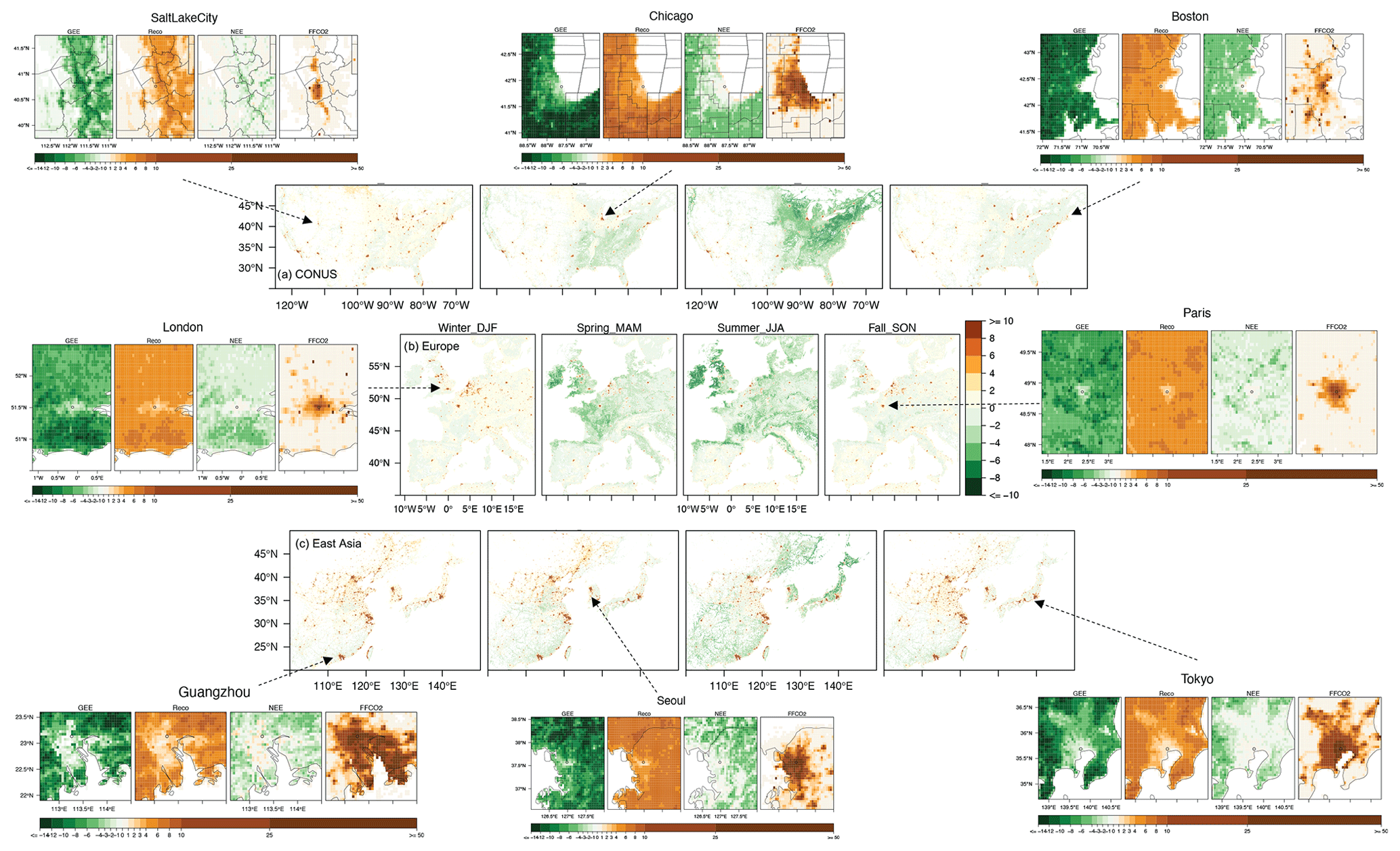
Figure 6The sums of seasonal mean SMUrF-based NEE and ODIAC-based FFCO2 [µmol m−2 s−1] for CONUS (a), western Europe (b), and East Asia (c) at 0.05∘ for 2018. Spatial distributions of the average GEE (−GPP), Reco, NEE, and FFCO2 from ODIAC over JJA 2018 are provided for eight cities (hereinafter zoomed-in panels). As an optional step, these fluxes can further be spatially downscaled to 1 km using MOD44B (Fig. S7).
We next zoom into fluxes at the city scale. SMUrF captures the increasing biospheric activities from urban cores to their rural surroundings inferred by gross ecosystem exchange (GEE is −GPP), Reco, and NEE components (eight zoomed-in panels in Fig. 6), as cities are usually associated with less vegetation coverage than their rural counterparts. The urban–rural difference in GEE over Salt Lake City, Boston, and Seoul is relatively small, in contrast to cities like Guangzhou and Tokyo. Since modeled Reco is partially driven by SIF-based GPP, the spatial variations of GEE and Reco appear alike to some extent. Even though GPP can be high over JJA 2018, summertime mean NEE remains small at urban cores, with values ranging from −1 to −2 µmol m−2 s−1. For Boston, the spatial distribution of GEE and Reco derived from SMUrF (Fig. 6) resembles what was reported using urbanVPRM (Fig. 2c in Hardiman et al., 2017). Reco from SMUrF exceeds ODIAC-based FFCO2 emissions over residential and rural areas away from urban cores (Fig. 6), which coincides with Decina et al. (2016), who reported an elevated rate of soil respiration approaching FFCO2 emissions in a residential area and forest to the west of an urban core. Yet, when it comes to interpreting observed CO2 concentrations, it is the net flux that should be compared against FFCO2. In short, biogenic fluxes have the potential to dominate the overall carbon flux exchange over residential and rural areas, while FFCO2 is the main controller within urban cores.
We further extend the analysis to 40 cities across multiple continents to see how CO2 fluxes vary between (1) urban and adjacent rural areas, (2) different cities, (3) the FF and NEE components, and (4) across seasons. Specifically, FFCO2 and NEE fluxes are averaged over urban and rural grid cells within a region around city centers. Here urban grids are simply defined as the “urban and build-up settlements” according to MCD12Q1, while rural grids contain all the natural counterparts (e.g., forests, grasslands, croplands) except for water, ice, and barren lands. In particular, we are interested in the seasonal variation (Sect. 3.1.1) and mean summertime diurnal cycle (Sect. 3.1.2) of these urban and rural fluxes. The diurnal cycles of FFCO2 are calculated using hourly scaling factors from Temporal Improvements for Modeling Emissions by Scaling (TIMES; Nassar et al., 2013) on top of monthly mean ODIAC-derived emissions. Note that emission temporal patterns provided by TIMES are climatological, based on a US gridded inventory by Gurney et al. (2009), and thus do not change in response to local environmental conditions, such as air temperature.
3.1.1 Seasonal variation
Stronger net biospheric uptake during growing seasons and a larger seasonal amplitude in NEE are more linked to rural grids than to urban grids as expected (Fig. 7a vs. b). Among the selected 40 cities, the top “wet” biologically active cities include Boston, Baltimore and DC, New York, Taipei, London, Paris, and Rio de Janeiro. By contrast, a few “drier” cities stand out, with the spatially averaged NEE over urban grids close to zero, such as Los Angeles, Phoenix, and Madrid (Fig. 7a). Besides NEE magnitude, cities reach their maximum net uptake at different times: e.g., June–July for most cities in the eastern US and East Asia (except for Taipei); a slightly earlier peak for most cities in the western US, western Europe, and Taipei; and January for cities in the Southern Hemisphere. For instance, minimum NEE is found in late May to June within and around London (Fig. 7a5), which is consistent with the seasonality of the posterior NEE fluxes reported for the UK from 2013 to 2014 (White et al., 2019).
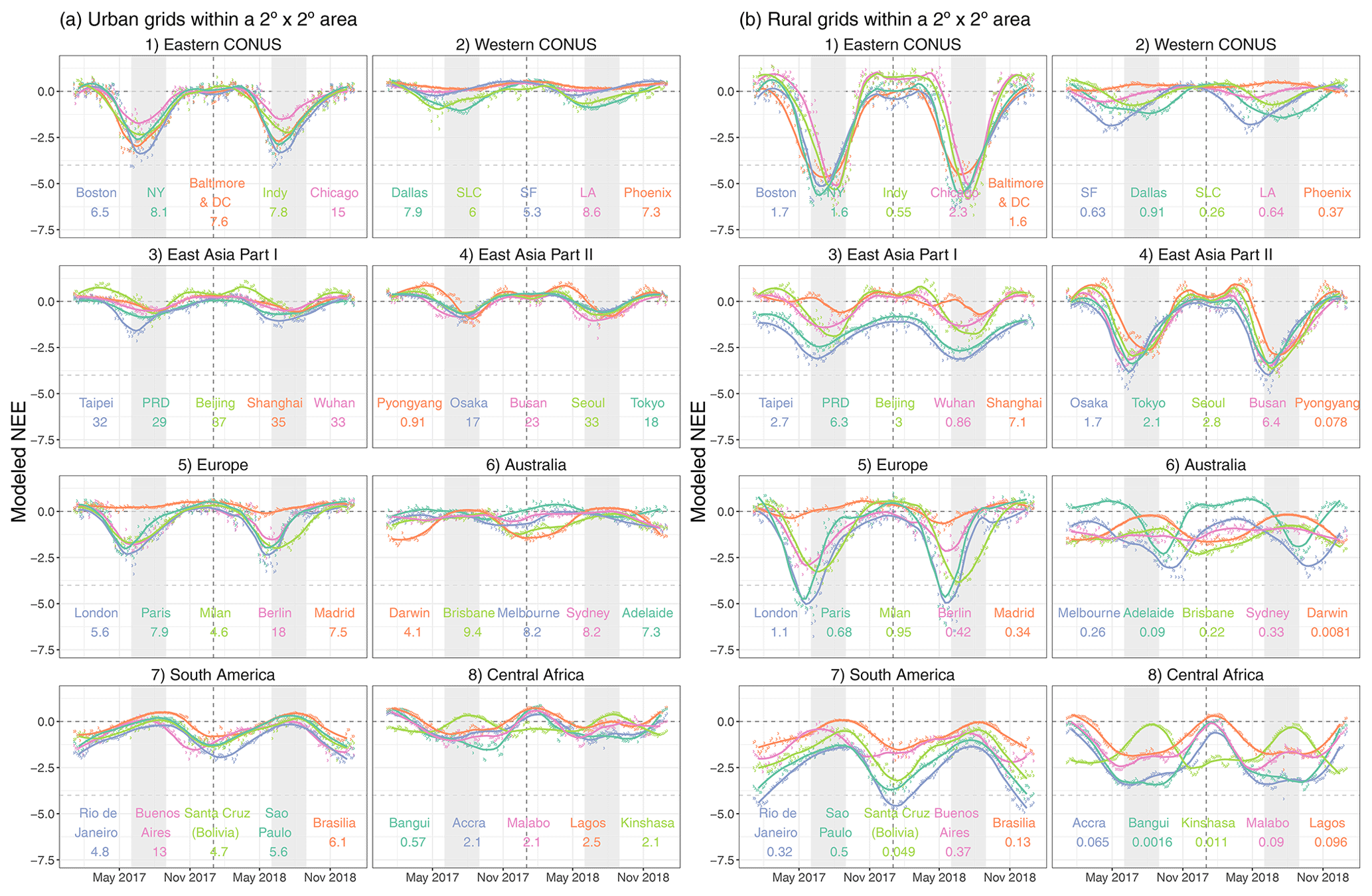
Figure 7A multi-city comparison of the spatially averaged NEE fluxes [µmol m−2 s−1] over urban (a) and rural (b) grid cells within a 2 2∘ area around the urban center for 2017–2018. We present the 4 d mean (in circles) and monthly mean (smoothed splines) NEE for 40 selected cities in CONUS, western Europe, East Asia, eastern Australia, South America, and central Africa. Light gray ribbons indicate the typical northern hemispheric summer months (June–August, JJA). The numbers below city names denote the spatially averaged fossil fuel CO2 emissions derived from ODIAC over the same grid cells as NEE.
Since FFCO2 emissions fluctuate less across seasons than NEE, we compare the magnitude of the seasonal amplitude of NEE relative to the annual mean FFCO2 emission (shown as numbers below city names in Fig. 7). Such a comparison helps inform the potential interference from the biosphere over cities when interpreting long-term CO2 observations, albeit without considering the atmospheric transport and the fact that the one single number for FFCO2 can be affected by large point-source emissions. As expected, most spatially averaged FFCO2 emissions over urban grids are stronger than the seasonal amplitude of NEE (Fig. 7a). Exceptions include Pyongyang and cities in central Africa whose seasonal NEE amplitudes approach their annual mean FFCO2 emissions, e.g., 2.0 vs. 2.5 µmol m−2 s−1 for Lagos. Things can get more complex if one tries to interpret FFCO2 signals from year-long observations over rural areas. Annual mean FFCO2 emissions for rural grids seldom exceed 2 µmol m−2 s−1, whereas seasonal amplitudes in the 4 d mean NEE often exceed 4 µmol m−2 s−1 (Fig. 7b), with a few exceptions in East Asia.
3.1.2 Diurnal cycle
With regard to the magnitude of hourly fluxes, FFCO2 emissions are negligible for rural grids (Fig. 8b). Intensive FFCO2 emissions ranging from 20 to 60 µmol m−2 s−1 dominate the total CO2 fluxes, even during noon hours for East Asian cities (Fig. 8a3–4). The urban biosphere over a few cities in the eastern US and Europe may take up a considerable amount of CO2, approaching or even exceeding FFCO2 emissions during noon hours in summer months. For instance, the peak value of summertime average NEE and FFCO2 fluxes over Boston is about −16 and 10 µmol m−2 s−1, respectively (Fig. 8a1), at the hourly scale.
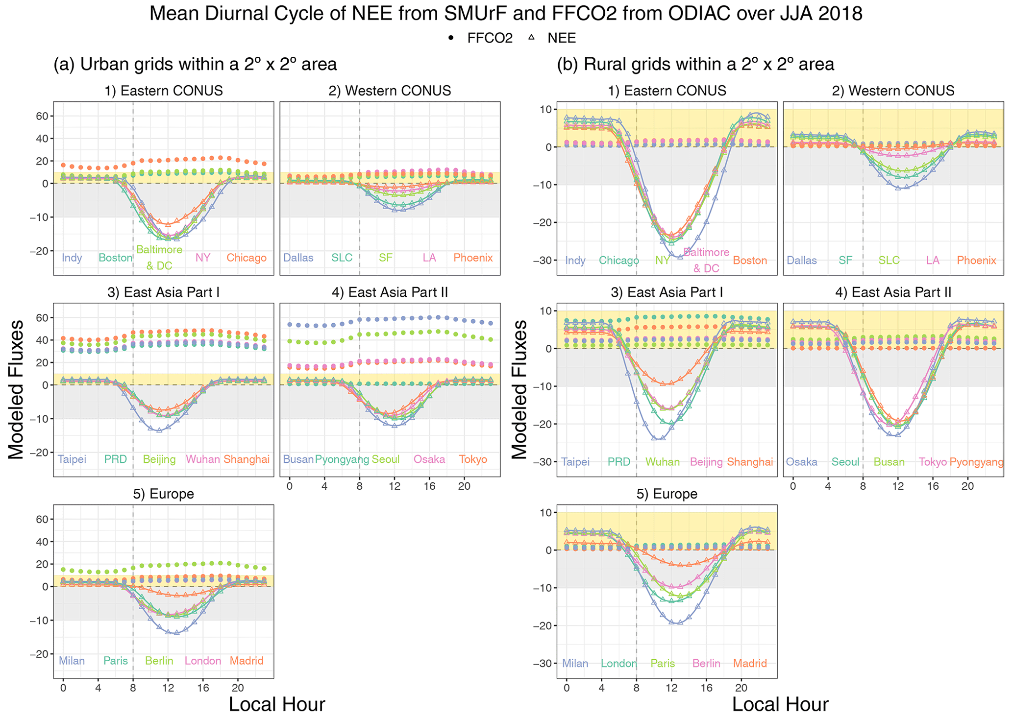
Figure 8A multi-city comparison of the average diurnal cycles of SMUrF-derived NEE fluxes (triangles and solid lines) and ODIAC–TIMES based FFCO2 (solid dots) [µmol m−2 s−1] over JJA 2018 for urban (a) and rural (b) grid cells within a 2 area around each urban center. Note that the y scales of positive and negative fluxes are different for panel (a) to better reveal the NEE fluxes, i.e., 0 to 60 µmol m−2 s−1 for positive fluxes and −20 to 0 µmol m−2 s−1 for negative fluxes. Light gray ribbons indicate the negative flux ranges from −10 to 0 µmol m−2 s−1, while light-yellow ribbons indicate the positive flux ranges from 0 to +10 µmol m−2 s−1. City names are labeled at the bottom of each panel.
With regard to the timing of hourly fluxes, NEE in most midlatitude cities starts to dip below zero at 07:00 or 08:00 local time (Fig. 8a), which is slightly later than the typical summertime sunrise hour of ∼ 06:00, with a lag associated with the time it takes for GPP to offset Reco. NEE reaches its minimum at different hours spanning from 11:00 to 13:00 among cities and rises back to zero at or before 18:00. In contrast, FFCO2 emissions start to rise largely due to morning traffic, stay elevated during daytime, and gradually decline between 20:00 and 21:00. As for Boston, SMUrF reported a similar NEE magnitude compared to urbanVPRM but with an hour delay during which NEE becomes negative (Fig. S9 vs. Fig. 3B3 in Hardiman et al., 2017), likely due to discrepancies in the hourly data that drive the hourly GPP fluxes.
3.2 Hourly flux comparisons
In this section, we will see how robust the modeled fluxes are at the hourly scale (Sect. 3.2.1–3.2.2) and how CO2 fluxes impact the CO2 concentrations downstream after considering atmospheric transport (Sect. 3.3). Specifically, simulated hourly mean NEE fluxes are extracted from the final gridded output fields and compared against measured NEE at EC sites from FLUXNET and INFLUX, which differs from the model–data comparison using directly computed daily fluxes in Sect. 2.5.
3.2.1 SMUrF vs. FLUXNET and INFLUX
We first evaluate modeled NEE against 67 EC tower sites from FLUXNET2015 in North America and Europe from 2010 to 2014 (Fig. 9). The correlation coefficient between simulated and measured hourly NEE ranges from 0.66 to 0.79 for most biome types except for open shrubland, likely due to limited amounts of data. Higher random and systematic uncertainties are associated with these hourly flux comparisons than direct daily validations shown in Sect. 2.5 (Fig. 5) given the larger flux magnitude along with errors propagated from GPP, Reco, and hourly downscaling. The mean bias of hourly NEE ranges from −1.51 µmol m−2 s−1 for grassland to +1.11 µmol m−2 s−1 for closed shrubland. Croplands are associated with the highest RMSE, which stems from their large flux magnitudes and inter-site variations in GPP–CSIF relationships (Fig. S1). The potential underestimation in 4 d average GPP over irrigated maize sites (e.g., US-Ne* as mentioned in Sect. 2.5) appears to be propagated into the NEE estimate (Fig. S10a). Yet, if all sites with the same biome are treated together, the timing and magnitude of the 3-month mean diurnal cycle of NEE from SMUrF resemble those from FLUXNET (Fig. S10b). Since each 0.05∘ model grid is possibly comprised of various biome types, areal fractions of the specific biome indicated by each EC site over the 0.05∘ model grid are provided as a reference in Fig. S11.
More importantly, we carried out independent NEE comparisons that leveraged four valuable EC sites from the INFLUX network over Indianapolis (Fig. 10a, Sect. 2.1.5). In 2018, observations at site no. 3 were affected by corn, while observations at site no. 2 were primarily influenced by soybeans, although site no. 2 was surrounded by mixed crops of soybeans and corn. As a result, site no. 3 shows a stronger observed uptake from mid-June to mid-July than site no. 2 (Fig. 10c) because corn is often associated with higher light saturation points and lower light compensation points, leading to higher light use efficiency and GPP than soybeans. Although the C3 : C4 fractional contribution was incorporated into the calculation of α (Sect. 2.2.1), SMUrF is unable to differentiate NEE at two adjacent crop sites found essentially in the same 0.05∘ model grid. The simulated NEE may agree better with the average observed NEE of two crop sites. Hourly measured NEE at crop sites ranges from −64.4 to +28.1 µmol m−2 s−1, while simulated values span from −66.7 to +12.1 µmol m−2 s−1 with a mean bias of −0.59 µmol m−2 s−1 and RMSE of 5.98 µmol m−2 s−1 over the entire observed window (Fig. 10c). Uncertainties and biases in the modeled hourly NEE based on these two crop sites outside Indianapolis are in proximity to those based on 11 FLUXNET crop sites (Fig. 10b vs. 9). Lastly, we focus on flux comparisons within Indianapolis. NEE fluxes at sites no. 1 and no. 4 exhibit a seasonally attenuated pattern but stronger biospheric activities in November and December compared to the crop sites (Fig. 10c). The correlation coefficient of hourly NEE fluxes between the model and observations is 0.75. Modeled mean diurnal cycles over JJA 2018 coincide with those from observations at urban vegetation sites (Fig. 10d). The spatial distribution of summertime average NEE from SMUrF can be found in Fig. S12.
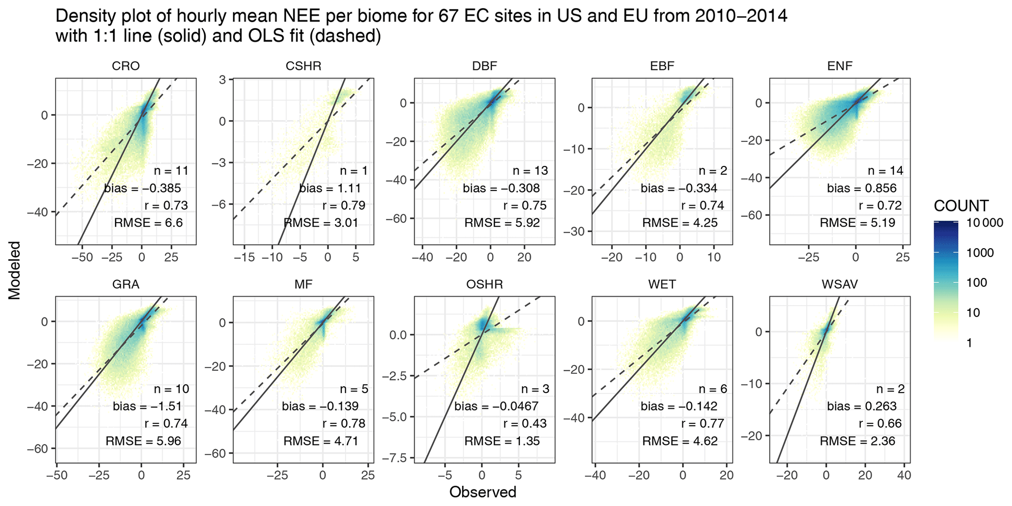
Figure 9Hourly flux comparisons between modeled NEE and measured NEE from FLUXNET are presented as a density plot for each biome. The number of EC sites per biome (n) and several error statistics including the mean bias, correlation coefficient (r), and root mean square error (RMSE) are printed in the bottom right corner of each panel.
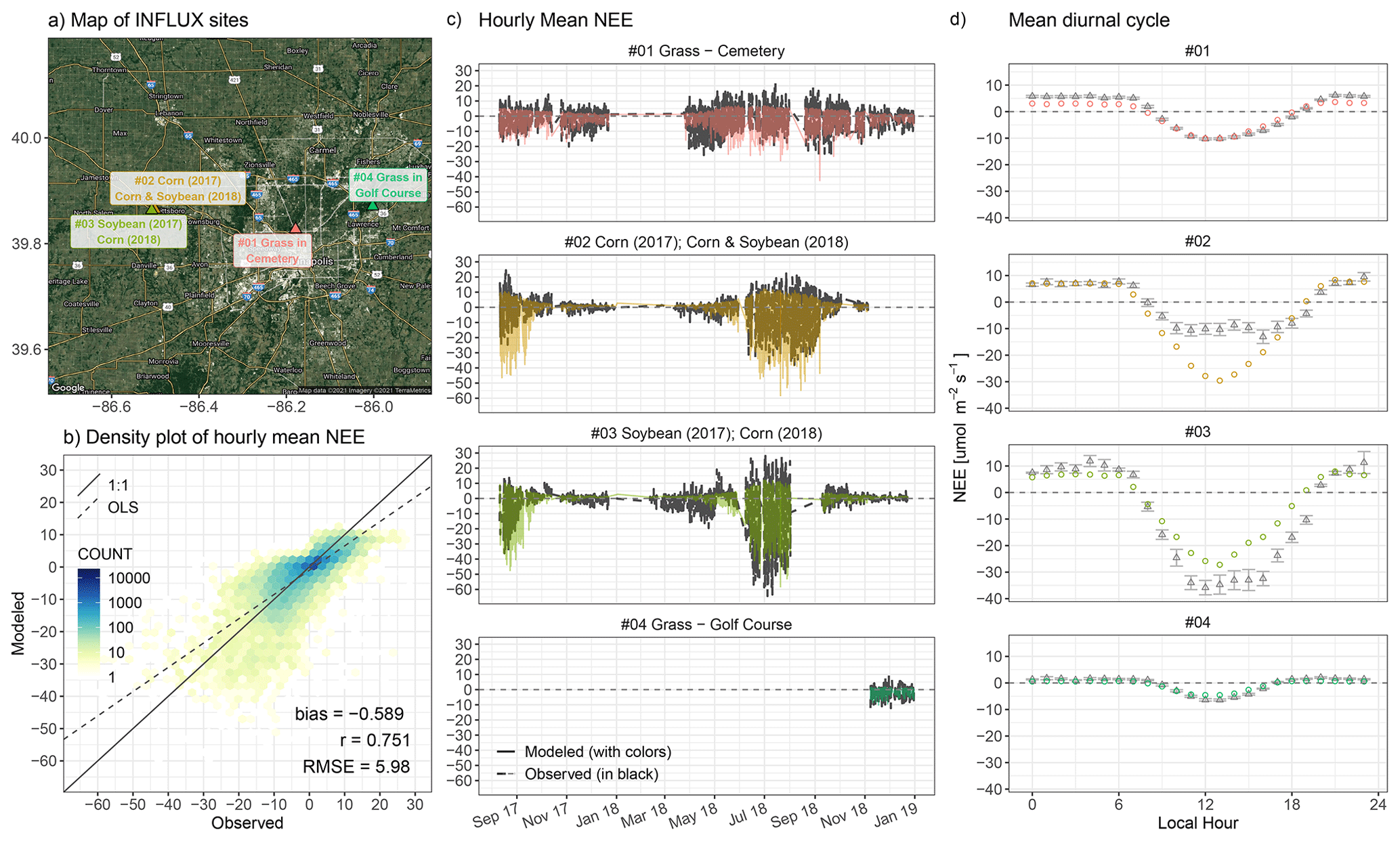
Figure 10NEE flux evaluation based on four EC towers from the INFLUX network around Indianapolis (a). Model–data flux comparisons at the hourly scale [µmol m−2 s−1] from August 2017 to December 2018 are shown as a density plot (b) and time series (c). Error statistics in hourly NEE including the mean bias, correlation coefficient (r), and root mean square error (RMSE) are printed in the bottom right corner of panel (b). (d) Mean diurnal cycle of observed NEE (black triangles) and modeled NEE (colored circles) over JJA for two cropland sites (sites no. 2 and no. 3) and the entire year of 2018 for urban vegetation sites (sites no. 1 and no. 4). For panel (c) and (d), model fluxes are shown as solid lines or circles with four colors indicating different sites, whereas measured fluxes are shown as black dashed lines or triangles. Supplementary information on the spatial map of modeled NEE and monthly mean NEE comparisons can be found in Fig. S12. Note that the underlying hybrid satellite image in panel (a) was generated using the ggmap R library with Google Maps (Map data © 2021 Imagery © 2021 TerraMetrics).
3.2.2 SMUrF vs. urbanVPRM for Los Angeles
The comparisons of SMUrF to dozens of EC sites have yet to offer much insight into the spatial distribution of urban CO2 fluxes. Therefore, we further compare SMUrF against urbanVPRM simulations (Sect. 2.1.5) at 30 m grid spacing over Los Angeles from July to September 2017. SMUrF and urbanVPRM agree with respect to the spatial distribution of estimated GEE fluxes, e.g., stronger uptakes over mountainous and residential areas to the northeast of Pasadena and San Bernardino and nearly zero uptake over the Moreno Valley to the south of Riverside and the LA basin (Fig. 11a). SMUrF simulates a stronger biospheric uptake than urbanVPRM across LA over JAS in 2017 (first column in Fig. 11a).

Figure 11(a) Spatial maps of mean GEE, Reco, and NEE fluxes [µmol m−2 s−1] from SMUrF and urbanVPRM over the greater Los Angeles region from July to September (JAS) in 2017. (b) Mean diurnal cycles of NEE fluxes over JAS 2017 between the two models. (c) Map of mean FFCO2 [µmol m−2 s−1] at 0.05∘ aggregated from the 1 km ODIAC product over JAS 2017. Main cities have been labeled on the maps including Los Angeles, Pasadena, Irvine, Riverside, and San Bernardino.
Both models incorporated observed GPP from EC sites for tuning their parameters but are driven with different spatial proxies (SIF vs. EVI and LSWI) with different model formulations. As one of the key improvements, urbanVPRM revises the initial VPRM-based Reco by incorporating impervious surface areas (ISAs), which in turn modify the air temperature over urban cores due to the urban heat island (TUHI) effect and affect estimated GPP as well as autotrophic and heterotrophic respiration. For example, RH can be reduced, while RA and GPP may be increased given enhanced TUHI over higher ISA regions in urbanVPRM. Regardless, TUHI-revised Reco in urbanVPRM still follows a simple function of air temperature. ISA is implicitly contained in SIF although not explicitly considered in SMUrF. Reco in SMUrF is driven not only by air temperatures but also soil temperatures and GPP. Thus, Reco in SMUrF appears to be more spatially correlated with its GPP. An overall higher Reco and more positive NEE are associated with SMUrF compared to urbanVPRM over LA (third column in Fig. 11a), which is attributed to methodological discrepancies in producing Reco. Similarly, the 3-month mean diurnal cycles of hourly NEE extracted from a few grids indicate stronger daily amplitudes according to SMUrF (Fig. 11b). Both models suggest that Pasadena, towards the northern end of the LA basin, is associated with a slightly stronger diurnal amplitude than downtown LA, with discrepancies in the hourly NEE during noon hours, likely because of differences in the data products from which PAR and SWrad are derived (e.g., cloud coverage and spatial resolution).
Despite the opposing signs between urbanVPRM- and SMUrF-modeled NEE over the LA basin, the overall biological activity (either net positive or negative) remains small, particularly when FFCO2 emissions are compared. As a quick analysis, we defined “downtown LA” as a rectangle with the lat–long boundaries 118.5–118∘ W and 33.9–34.1∘ N and removed one grid cell with intensive FFCO2 emissions from consideration (likely due to point sources; Fig. 11c). The average FFCO2 over JAS 2017 within downtown LA is ∼ 12.1 µmol m−2 s−1, while differences in NEE between the two biogenic models remain small at ∼ 0.41 µmol m−2 s−1.
3.3 Urban–rural gradient in XCO2.ff and XCO2.bio
After presenting the hourly NEE evaluations and urban–rural contrast around 40 cities, we examined the imprint of urban–rural NEE contrasts in CO2 concentrations. As described in Sect. 2.6, we analyzed OCO-2 XCO2 observations over a few cities and accounted for the atmospheric transport between upwind carbon sources and sinks and downwind satellite soundings as reflected by X-STILT's column footprints (Fig. 12a). Only places with nonzero footprints and nonzero fluxes contribute to downwind XCO2 anomalies, which can be visualized by the spatial contribution of XCO2.ff enhancements and XCO2.bio anomalies in Fig. 12cd. The sum of those spatially explicit XCO2 contributions serves as the total anthropogenic or biogenic XCO2 anomalies per receptor (Fig. 12b).

Figure 12Demonstration of the application of SMUrF in the context of column CO2 measurements for an OCO-2 overpass at 17:00 UTC on 7 July 2018 to the west of Boston. The time-integrated column footprints [ppm/(µmol m−2 s−1)] originating from dozens of receptor locations have been integrated along latitude (a). The wind was blowing from the urban center of Boston onto the satellite swath. (c–d) Spatially explicit XCO2 contributions from ODIAC-based FFCO2 and SMUrF-based NEE (XCO2.ff and XCO2.bio in ppm). Note that the spatial footprint (a) and the spatial contribution of XCO2.ff (c) are plotted in log10 scale, with small values < 10−6 ppm/(µmol m−2 s−1) displayed in light gray. The upwind contributions with respect to a column receptor are summed up, which leads to the total modeled XCO2.ff or XCO2.bio anomalies per receptor (orange or green dots in panel b). Light orange and green ribbons indicate the urban-enhanced and background latitude range, following the approach in Wu et al. (2018) (also demonstrated in Fig. S13). Note that the underlying hybrid maps in panels (a), (c), and (d) were generated using the ggmap R library with Google Maps (Map data © 2021 Imagery © 2021 TerraMetrics). (e) An example of incorporating ΔXCO2.bio into the background estimates. The screened observed XCO2 values (QF = 0; gray triangles) are averaged in bins to match the locations of X-STILT receptors (black triangles). The dark and light green lines indicate the constant and bio-adjusted XCO2 background. Differences between two XCO2.bg values indicate the ΔXCO2.bio, which is calculated by subtracting the mean XCO2.bio within the rural range from all the simulated XCO2.bio values along the swath. The FFCO2 enhancements are further added to the two different background values to arrive at the total modeled XCO2 (orange and purple lines).
Boston is the main case study here as its anthropogenic and biogenic fluxes have been extensively studied in previous research (Decina et al., 2016; Hardiman et al., 2017; Sargent et al., 2018), notwithstanding the small number of qualified OCO-2 tracks. On 7 July 2018, the northeasterly wind transported air from Boston to downwind satellite soundings with an overpass time of ∼ 17:00 UTC or 13:00 LT (Fig. 12a). Over the near-field area immediately around satellite soundings, most biogenic contributions stayed negative due to daytime photosynthetic uptake (green in Fig. 12d) where strong surface influences are found (Fig. 12a). During the few hours prior to 13:00 LT, air parcels within the planetary boundary layer began to encounter net biogenic release away from the receptors, leading to slightly positive biogenic contributions to XCO2 (light yellow in Fig. 12d). Yet, strong negative near-field anomalies prevail over the slightly positive far-field anomalies, resulting in total negative XCO2.bio at the receptors spanning from −2 to −0.3 ppm (green dots in Fig. 12b). The convolution between footprints and FFCO2 emissions is simpler and always yields positive enhancements (Fig. 12c), especially over soundings from 41.7 to 42.3∘ N with XCO2.ff enhancements of up to 0.6 ppm (orange dots in Fig. 12b).
We then take a closer look at the modeled XCO2 anomalies along latitude (Fig. 12b). XCO2 anomalies to the south of the urban peak are close to zero due to minimal influences from either FFCO2 or NEE. Moving northward, soundings started to experience intensive biogenic activities that lead to XCO2.bio anomalies of up to −2 ppm. Due to a less active urban biosphere than its surrounding vegetation, a rise in XCO2.bio has been spotted centered at ∼ 41.9∘ N relative to the adjacent latitude bands centered at ∼ 41.7 or 42.2∘ N. That being said, the urban–rural gradient in XCO2.bio anomalies (hereinafter ΔXCO2.bio) can exceed 0.5 ppm, which is comparable to the maximum XCO2.ff of 0.6 ppm. We will discuss the implications of this urban–rural bio-gradient ΔXCO2.bio in the context of the total measured XCO2 in Sect. 4.1 (Fig. 12e).
Clearly, ΔXCO2.bio can vary with location and the time of day or year when measurements are taken. We studied a few more OCO-2 tracks near Indianapolis, Salt Lake City, and Rome given their different surrounding vegetation types (Fig. 13). These summertime tracks were chosen given their richness in screened soundings (quality flag of 0), which facilitates the X-STILT modeling. Although the OCO-2 track is adjacent to Indianapolis at 18:00 UTC on 13 July 2018, upwind regions are located to the east of the soundings and away from Indianapolis, leading to minimal XCO2.ff anomalies and strong biospheric uptake with XCO2.bio below −2 ppm (Fig. 13ab). A strong influence of the surface land is concentrated within the Salt Lake Valley on 25 June 2018, leading to a maximum XCO2.ff of 0.5 ppm and XCO2.bio with a comparable magnitude but negative sign (Fig. 13ef). For Rome, strong footprints to the southwest of the city center interact with positive NEE, giving rise to XCO2.bio anomalies of up to 1.5 ppm over 42–42.5∘N where XCO2.ff is equally significant (Fig. 13j). To sum up, XCO2.bio anomalies can be associated with either sign and an absolute magnitude of up to 2.5 ppm during growing seasons, as seen in the cases of Indianapolis and Boston. The urban–rural bio-gradient ΔXCO2.bio is smaller, with maximum values ranging from 0.6 to 1.0 ppm among our limited cases (second column in Fig. 13). Based on the limited cases, XCO2.bio anomalies are normally less negative (more positive) within the urban-enhanced region, serving as a peak that coincides with the XCO2.ff peak. More cities and satellite tracks, accompanied by comprehensive error analyses, should be examined in the future to verify these statements.

Figure 13Similar to Fig. 12a–d but for three different OCO-2 tracks, including 18:00 UTC on 13 July 2018 to the east of Indianapolis (2018071318; first row, a–d), 20:00 UTC on 25 June 2018 right over Salt Lake City (2018062520; second row, e–h), and 12:00 UTC on 15 June 2017 near Rome, Italy (2017061512; third row, i–l). The meteorological fields that drove those simulations are 3 km HRRR for US cities and 0.5∘ GDAS fields for Rome. Note that the underlying hybrid satellite images in the first, third, and fourth columns were generated using the ggmap R library with Google Maps (Map data © 2020 Imagery © 2020 TerraMetrics).
We now discuss some applications and limitations of SMUrF. In particular, we examine how an urban–rural gradient in XCO2.bio may alter the interpretation of XCO2 observations during growing seasons.
4.1 Implications on background XCO2 determination
As the extraction of urban emissions from column measurements can be sensitive to the background definition (e.g., Wu et al., 2018), we illustrate the impact of the urban–rural gradient in XCO2.bio during the growing season in the context of background determinations. Let us consider the background XCO2 (XCO2.bg) defined as the average of observations over a region unaffected by urban emissions. Observed enhancements are then calculated as levels of XCO2 elevated above XCO2.bg. This constant XCO2.bg reasonably represents the XCO2 portion unaffected by urban emissions during non-growing seasons for most places (Wu et al., 2018). However, this background definition might implicitly neglect the variation in biospheric XCO2 anomalies between the urban-enhanced and background region. Again, it is the gradient in XCO2.bio, not its absolute level, along satellite tracks that modifies the background value.
The goal, then, becomes to create a latitude-dependent background – XCO2.bg (lat) in Eq. (3) – that integrates the adjustment of the urban–rural biospheric gradient (ΔXCO2.bio). To quantify the ΔXCO2.bio correction term, we average XCO2.bio within the background latitude band (XCO2.bio.bg) and subtract it from the latitude-varying XCO2.bio. The correction term is then added to the constant background (XCO2.bg.const) to yield a latitudinally varying, bio-adjusted background:
Recall that XCO2.bio (lat) represents the modeled biospheric anomalies using SMUrF and X-STILT (Sects. 2.6 and 3.3).
To facilitate visualization and understanding of ΔXCO2.bio and the bio-adjusted background, let us return to the Boston case (Fig. 12). Following the “overpass-specific approach” proposed in Wu et al. (2018), we estimated the urban plume (black curve in Fig. S13a) and defined the background latitude range of 42.26–42.76∘ N (light green ribbon in Fig. 12e). The constant background is 403.37 ppm (dark green line in Fig. 12e) with an uncertainty of 1.03 ppm containing both retrieval errors and observational noise (Fig. S13b). The mean XCO2.ff and XCO2.bio anomalies within the background region are 0.23 ppm and −1.41 ppm, respectively. After integrating the bio-gradient ΔXCO2.bio, a new bio-adjusted background varies along latitude (light green line in Fig. 12e). If modeled XCO2.ff is added to the bio-adjusted background, the resultant total XCO2 better reproduces the latitudinal variations of the measured mean values (Fig. 12e). Both the observed XCO2 and modeled XCO2 with the ΔXCO2.bio correction term exhibit dips in XCO2 on both sides outside the urban peak, which is missing from the model result using the constant background (orange line in Fig. 12e).
A more comprehensive error analysis of various modeled and observed errors is needed to draw further quantitative conclusions from the model–data XCO2 comparison. For instance, modeled XCO2 appears to extend wider latitudinally with a lower amplitude and a small latitude shift of ∼ 0.1∘ compared to observed XCO2 (purple line versus black triangles in Fig. 12e), likely due to a bias in wind speed and direction. Nonetheless, neglecting the latitudinal and spatial gradient in biogenic XCO2 anomalies given gradients in NEE can affect the extracted urban signal and inferred FFCO2 emissions.
4.2 Limitations and future improvement
This study aims to offer a model representation of biogenic CO2 fluxes to help improve the CO2 flux partitioning over cities worldwide. SMUrF takes advantage of SIF to estimate GPP from urban to rural areas and incorporates multiple predictors to estimate Reco using a neural network approach. Here we identify several model limitations and room for future improvements.
The adoption of SIF has dramatically benefited the GPP calculation over urban areas around the globe, as non-vegetated surfaces within the satellite footprint do not contribute to observed signals. However, the main caveat lies in the assumption of a linear GPP–SIF relationship and one set of constant α values across all seasons used in SMUrFv1. Previous research (Magney et al., 2020; Miao et al., 2018; Wohlfahrt et al., 2018; Yang et al., 2018) revealed the divergence of the empirical linear GPP–SIF relation at sub-diurnal and leaf scales, as well as under certain environmental conditions (low light or high light and stress), owing to competing fluorescence, photochemical, and non-photochemical pathways for the absorbed light (Magney et al., 2020). For example, Yang et al. (2018) suggest considering additional environmental and biophysical factors related to the modeling of light use efficiency, e.g., relative humidity, cloudiness, and growth stage of crops, to improve SIF-based GPP estimates. Although multiple studies have shown a dependence of the linear slope on PFT (e.g., Guanter et al., 2012; Sun et al., 2017; Turner et al., 2021), further research is needed to understand the scale dependence of the GPP–SIF relation and determine if an inflection point for linearity exists. Given noise and uncertainty in the CSIF product and EC tower data across multiple continents, we apply a simple linear regression fit and let the uncertainty analysis incorporate deviations from the linear assumption. Future iterations of SMUrF can test alternative statistical fits with physical fundamentals or expand the GPP–SIF slopes across seasons and new urban land cover maps (e.g., Coleman et al., 2020).
Mixed pixels are difficult to account for in heterogenous urban environments without much information on the local biosphere. As a general solution that can be widely applied to cities around the world, we derived and utilized the relationship between relative tree fractions and AGB. This relationship is a simplification proposed from high-resolution land cover data over Los Angeles. Fortunately, recent work using high-resolution airborne and satellite imagery demonstrates that urban land cover mapping capabilities are improving (e.g., Coleman et al., 2020). Other advanced space sensors provide SIF retrieval with broader coverage over cities, land surface temperatures, biomass, and canopy structures of forests at an unprecedented spatiotemporal resolution (Stavros et al., 2017). Examples of such satellite sensors include OCO-3 (Eldering et al., 2019), the ECOsystem Spaceborne Thermal Radiometer Experiment (ECOSTRESS; Fisher et al., 2020), and the Global Ecosystem Dynamics Investigation lidar (GEDI; Duncanson et al., 2020), all on board the International Space Station. These cutting-edge and future data streams may improve the approximation of tree types and fraction over cities and flux estimates in SMUrF.
SMUrF parameters can be fine-tuned for more localized applications, such as using higher-resolution shortwave radiation or PAR data with higher accuracy in cloud cover estimates. Further, the reference temperature used in this work (30 ∘C) can be a bit higher than that (20 ∘C) used in the calculation of maintenance respiration and (25 ∘C) in the calculation of heterotrophic respiration in the Community Land Model (CLM). The Q10 parameter (here 1.5) also varies significantly in space and time. Moreover, a few second-order ecological and environmental variables may affect biogenic fluxes. For example, we have tried adding soil moisture as an explanatory variable into the Reco training system, but the improvement in model performance is not that evident.
It is a more challenging shortcoming that current flux estimates in SMUrF over cities still rely on relationships derived from observations over natural biomes. Urban trees are found to possess different characteristics than natural trees (Smith et al., 2019), which poses a difficult task for biospheric models without more dedicated observations and a mechanistic understanding of the urban environment. Anthropogenic moisture input (i.e., urban irrigation) has been found to effectively influence urban biogenic fluxes, particularly over (semi)arid residential areas (Johnson and Belitz, 2012; Vahmani and Hogue, 2014; Miller et al., 2020). Although we currently rely on SIF to pick up possible irrigation effects on GPP, it would be interesting to explore the linkage between water and carbon fluxes in future analyses.
Because atmospheric CO2 concentrations measured from satellites are mainly influenced by anthropogenic and biogenic carbon fluxes a few hours to days ahead of the overpass time, this work focused on presenting and evaluating diurnal and seasonal CO2 fluxes. Biogenic CO2 fluxes at other moments, e.g., their interannual variations and trends, may require further investigations. We hope to examine more cities and different times of the day in future studies to better quantify the relative biogenic and anthropogenic contributions to XCO2 anomalies. Incorporating uncertainties in biogenic fluxes and resultant XCO2.bio is needed for future top-down studies with the aim of quantifying urban signals, especially over growing seasons.
Lastly, we summarize the potential applications of SMUrF as follows.
-
Improve the separation between biogenic and anthropogenic CO2 fluxes for urban studies. Regardless of the exact approach adopted for background definition, researchers can combine atmospheric transport models with fluxes from SMUrF to get estimates of the CO2 anomalies due to biogenic flux exchanges, as shown in Sect. 4.1.
-
Fill in the urban gap and assist regional flux inversions. The state-of-art terrestrial models that go into flux inversions usually include global models with relatively coarse resolution (e.g., 4∘ by 5∘), with possible downscaling approaches. At the other end of the spectrum are highly localized models at fine resolution that sometimes require customization for individual cities. SIF-based fluxes from SMUrF may help bridge the gap between the continental scale and the urban scale, with reasonable fine resolution and regional to global coverage.
-
Understand how urbanization modifies the planet and environment. SMUrF offers a quick solution to biogenic fluxes within urban areas and their rural surroundings, which provides insights on how biogenic CO2 fluxes vary among cities with different urban planning and emissions.
We carried out two tests to verify the accuracy and capability of CSIF. Firstly, CSIF is compared against a newly developed SIF product from TROPOMI over the contiguous United States (CONUS) from June to August in 2018 (Turner et al., 2020, 2021). This downscaled TROPOMI-based SIF product is initially available at 500 m and then averaged to 0.05∘ for the comparison. Due to the discrepancies in the reported SIF retrieval wavebands between OCO-2 (757 and 771 nm) and TROPOMI (740 nm), the OCO-2 based CSIF (757 nm) is scaled by an empirical scaling factor of 1.56 (Köhler et al., 2018) to yield comparison with TROPOMI SIF at the far-red SIF peak of 740 nm. Note that this scaling factor of 1.56 is only applied here for model comparisons and not for flux calculations. OCO-2 based CSIF and TROPOMI-based SIF both see high biological activity over the eastern CONUS and agree well spatially (Fig. S2). Model–model mismatch can be attributed to their different approaches and adopted observations. For example, CSIF uses broadband reflectances as indicators, whereas the downscaled TROPOMI SIF product benefits from TROPOMI's wider and denser spatial coverage. Nevertheless, CSIF-based α values (mostly > 20 (µmol m−2 s−1) (mW m−2 sr−1 nm) are higher than TROPOMI-based α, ranging from 13.5 to 18 (µmol m−2 s−1) (mW m−2 sr−1 nm−1)−1 as reported in Turner et al. (2020, 2021), which potentially compensate for the SIF mismatch.
We also relate CSIF to vegetated and impervious fractions with a spatial resolution of 10 km from the World Urban Database and Access Portal Tools (WUDAPT) project (Ching et al., 2018) for a few available US cities. WUDAPT is “an international community-generated urban canopy information and modeling infrastructure to facilitate urban-focused climate, weather, air quality, and energy-use modeling application studies” (Ching et al., 2018). The local climate zones (LCZs) provided by WUDAPT contain 10 specific classifications for the urban areas and 7 natural types with characterizations of surface properties and structures (e.g., building and tree height and density) as well as surface cover (pervious vs. impervious) (Stewart and Oke, 2012). Each LCZ classification is associated with a range of fractions for impervious land, buildings, and vegetation, such as 40 %–60 % of impervious percentage for compact high-rise class (Ching et al., 2018). We calculated the mean impervious and vegetated fractions for every LCZ and projected those fractions to CSIF's grids. Consequently, the spatial gradient of CSIF coincides with that of vegetated fractions estimated from WUDAPT, as suggested by the increasing trend moving away from urban cores (Fig. S3). Thus, CSIF nicely reveals the urban–rural contrast in biological activities.
Since CSIF nicely mimics the urban–rural gradient, additional information about vegetated and impervious fractions was not necessary in the calculation of α for every 500 m urban grid. For instance, if half of the 0.05∘ urban grid cell is covered by impervious land with the rest covered by DBFs, the SIF of this grid cell would already be lower than the SIF of a grid cell fully covered by DBFs. Thus, instead of calculating a weighted mean α using slopes and land fractions of DBF and impervious land (whose α=0), we only need to assign the α of DBF to this particular 500 m urban grid. Otherwise, the resultant urban GPP (CSIF ×α) could be underestimated by “double counting” of the impervious fraction in both SIF and α.
As introduced in Sect. 2.3, we have tested three ways to predict Reco by applying the following:
- M1.
one NN model trained using data points with all biomes to 0.05∘ grids, except for water, ice, and barren land, without considering sub-grid-cell variations in land cover types;
- M2.
one NN model with biome as well as the month and season of the year as additional categorical variables (with one-hot encoding); and
- M3.
multiple biome-specific NN models to 500 m grids with different biomes and aggregating predicted Reco to 0.05∘.
Technically speaking, we tried both the built-in R package Neuralnet (Fritsch et al., 2016) and the R interface for Keras (Falbel et al., 2019), which is a high-level neural network API based on the back end including TensorFlow to build NN models. Although M1 benefits from more sample data and shorter processing time in predicting Reco without matching NN models with land cover types at 500 m, the M2 approach is physically more meaningful as the temperature dependence of respiration may vary among different vegetation species. In particular, being able to resolve sub-grid-cell variations and different vegetation fractions (processed during GPP estimates, Sect. 2.2.2) facilitates a more reasonable Reco calculation over urban areas. Note that modeled Tair and Tsoil have been bilinearly interpolated from their initial grid spacings onto the required grid spacing. In the end, we used the last M3 approach given its better performance.
Before training neural network models, we removed a few flux sites with relatively large RMSE values between modeled and observed GPP to avoid erroneous information being transformed into the training process of Reco (Fig. S14). All explanatory and response variables have been linearly normalized to values in the range [0, 1] based on their maximum and minimum values before training. Adjusting the raw data to a common scale may dramatically speed up the training process and avoid a situation in which the predicting variable appears to be more sensitive to one of the response variables. To determine the hyper-parameters that work the best on our data and help avoid underfitting or overfitting situations, we carried out a 5-fold cross-validation (Fig. S15). That being said, 80 % of the data serves as the training set, with the remaining 20 % as the validation set. The 5-fold cross-validation can be viewed as repeated holdouts, and the average errors will be calculated after five different holdouts. The main hyper-parameter tested here is the number of neurons (8, 16, 32, or 64 neurons per layer) for a two-layer model. The overall RMSE and loss function between predicted and observed Reco in the validating set turn out to be similar for different numbers of neurons. In addition, loss functions in the training and validating sets appear to be similar, implying no strong sign of overfitting.
The source codes of SMUrF with the latest changes and the SMUrF flux output are available at http://dienwu.me/gmd2021 (last access: 7 September 2020). The exact version of the SMUrF model used in this work is archived on Zenodo (https://doi.org/10.5281/zenodo.4018123, D. Wu, 2020).
Instructions for running SMUrF. The user should start with main scripts of main_script_*.r in sequence for computing gridded GPP, Reco, and NEE, since the calculation of Reco using main_script_Reco.r relies on GPP generated using main_script_GPP.r. Model-related subroutines written in R/3.6.1 are stored in SMUrF/r/src with model-required dependences in SMUrF/data. For most of the cases, the user does not need to modify these subroutines. Model developments are ongoing, so please contact the corresponding author to obtain model outputs for other regions and/or cities.
Required input data products for driving SMUrF (data citation; parameter name in the model script).
-
Clear-sky SIF provided by CSIF (Zhang et al., 2018; csif.cpath)
-
AGB from GlobBiomass (Santoro et al., 2018; agb.path)
-
MCD12Q1 v006 (Friedl and Sulla-Menashe, 2019; lc.path) accessed from the Application for Extracting and Exploring Analysis Ready Samples (AρρEEARS); see README.md on the GitHub repository for information on how to download the exact format that SMUrF requires
-
Hourly air temperature and shortwave radiation downwards from ERA5 reanalysis (Copernicus Climate Change Service Information, 2017; TA* and SSRD*)
Other important data products used in this paper (not prerequisites for driving SMUrF) include
-
the high-resolution 60 cm NAIP-based urban land cover classification product (Coleman, 2020) from Mendeley data,
-
the ODIAC emission data product available from the Global Environmental Database hosted by the Center for Global Environmental Research at the National Institute for Environmental Studies (Oda and Maksyutov, 2015), and
-
EC measurements from FLUXNET2015 (Pastorello et al., 2017).
The supplement related to this article is available online at: https://doi.org/10.5194/gmd-14-3633-2021-supplement.
DW and JCL designed the study, and DW is responsible for model scripts. JCL and HD offered constructive insights regarding the construction and development of SMUrF. JCL, TO, and EAK contributed to the design of model results presentation. VY and NP provided the urbanVPRM model outputs for LA for flux comparison with SMUrF. All authors contributed to the editing of the final paper.
The authors declare that they have no conflict of interest.
The resources and support from the Center for High-Performance Computing at the University of Utah are gratefully acknowledged. A portion of this research was carried out at the Jet Propulsion Laboratory, California Institute of Technology, under a contract with the National Aeronautics and Space Administration. We are grateful to Ken Davis and Kai Wu at Penn State University for sharing INFLUX data and providing constructive comments on this paper. We acknowledge Alex Turner at the University of Washington for sharing the downscaled TROPOMI SIF data over the entire CONUS from June to August 2018. We thank Yao Zhang at the Lawrence Berkeley National Laboratory for sharing the 0.05∘ CSIF fields and for helpful discussions. Dien Wu also appreciates assistance from Guannan Wei (Purdue University) and Benjamin Fasoli (University of Utah) on the construction and evaluation of neural network models as well as discussions with Liyin He (Caltech) on the C3 C4 partitioning. Lastly, we appreciate all the constructive feedback from the two reviewers.
This research has been supported by the National Aeronautics and Space Administration (grant nos. NNX15AI40G, NNX15AI41G, NNX15AI42G, NNX14AM76G, 80NSSC18K1307, 80NSSC18K1313, 80NSSC19K0196, 80NSSC20K0010, and 80NSSC19K0093). Vineet Yadav and Nicholas C. Parazoo acknowledge funding from the NASA OCO-2 Science Team under grant number 17-OCO2-17-0025.
This paper was edited by Leena Järvi and reviewed by Youngryel Ryu and Taylor Jones.
Chen, J., Zhao, F., Zeng, N. and Oda, T.: Comparing a global high-resolution downscaled fossil fuel - CO2 emission dataset to local inventory-based estimates over 14 global cities, Carbon Balance Manag., 15, 1–15, https://doi.org/10.1186/s13021-020-00146-3, 2020.
Ching, J., Mills, G., Bechtel, B., See, L., Feddema, J., Wang, X., Ren, C., Brorousse, O., Martilli, A., Neophytou, M., Mouzourides, P., Stewart, I., Hanna, A., Ng, E., Foley, M., Alexander, P., Aliaga, D., Niyogi, D., Shreevastava, A., Bhalachandran, P., Masson, V., Hidalgo, J., Fung, J., Andrade, M., Baklanov, A., Dai, W., Milcinski, G., Demuzere, M., Brunsell, N., Pesaresi, M., Miao, S., Mu, Q., Chen, F., and Theeuwesits, N.: WUDAPT: An urban weather, climate, and environmental modeling infrastructure for the anthropocene, B. Am. Meteorol. Soc., 99, 1907–1924, https://doi.org/10.1175/BAMS-D-16-0236.1, 2018.
Coleman, R. W.: Southern California 60-cm Urban Land Cover Classification, Mendeley Data, V1, https://doi.org/10.17632/zykyrtg36g.1, 2020.
Coleman, R. W., Stavros, E. N., Yadav, V., and Parazoo, N.: A Simplified Framework for High-Resolution Urban Vegetation Classification with Optical Imagery in the Los Angeles Megacity, Remote Sensing, 12, 2399, https://doi.org/10.3390/rs12152399, 2020.
Copernicus Climate Change Service (C3S): ERA5: Fifth generation of ECMWF atmospheric reanalyses of the global climate. Copernicus Climate Change Service Climate Data Store (CDS), available at: https://cds.climate.copernicus.eu/cdsapp#!/home (last access: 14 April 2020), https://doi.org/10.24381/cds.bd0915c6, 2017.
Crisp, D., Fisher, B. M., O'Dell, C., Frankenberg, C., Basilio, R., Bösch, H., Brown, L. R., Castano, R., Connor, B., Deutscher, N. M., Eldering, A., Griffith, D., Gunson, M., Kuze, A., Mandrake, L., McDuffie, J., Messerschmidt, J., Miller, C. E., Morino, I., Natraj, V., Notholt, J., O'Brien, D. M., Oyafuso, F., Polonsky, I., Robinson, J., Salawitch, R., Sherlock, V., Smyth, M., Suto, H., Taylor, T. E., Thompson, D. R., Wennberg, P. O., Wunch, D., and Yung, Y. L.: The ACOS CO2 retrieval algorithm – Part II: Global XCO2 data characterization, Atmos. Meas. Tech., 5, 687–707, https://doi.org/10.5194/amt-5-687-2012, 2012.
Davis, K. J., Deng, A., Lauvaux, T., Miles, N. L., Richardson, S. J., Sarmiento, D. P., Gurney, K. R., Hardesty, R. M., Bonin, T. A., Brewer, W. A., Lamb, B. K., Shepson, P. B., Harvey, R. M., Cambaliza, M. O., Sweeney, C., Turnbull, J. C., Whetstone, J., and Karion, A.: The Indianapolis Flux Experiment (INFLUX): A test-bed for developing urban greenhouse gas emission measurements, Elementa, 5, 21, https://doi.org/10.1525/elementa.188, 2017.
Decina, S. M., Hutyra, L. R., Gately, C. K., Getson, J. M., Reinmann, A. B., Short Gianotti, A. G., and Templer, P. H.: Soil respiration contributes substantially to urban carbon fluxes in the greater Boston area, Environ. Pollut., 212, 433–439, https://doi.org/10.1016/j.envpol.2016.01.012, 2016.
Dietze, M. C., Vargas, R., Richardson, A. D., Stoy, P. C., Barr, A. G., Anderson, R. S., Arain, M. A., Baker, I. T., Black, T. A., Chen, J. M., Ciais, P., Flanagan, L. B., Gough, C. M., Grant, R. F., Hollinger, D., Izaurralde, R. C., Kucharik, C. J., Lafleur, P., Liu, S., Lokupitiya, E., Luo, Y., Munger, J. W., Peng, C., Poulter, B., Price, D. T., Ricciuto, D. M., Riley, W. J., Sahoo, A. K., Schaefer, K., Suyker, A. E., Tian, H., Tonitto, C., Verbeeck, H., Verma, S. B., Wang, W., and Weng, E.: Characterizing the performance of ecosystem models across time scales: A spectral analysis of the North American Carbon Program site-level synthesis, J. Geophys. Res.-Biogeo., 116, G04029, https://doi.org/10.1029/2011JG001661, 2011.
DiMiceli, C., Carroll, M., Sohlberg, R., Kim, D., Kelly, M., and Townshend, J.: MOD44B MODIS/Terra Vegetation Continuous Fields Yearly L3 Global 250m SIN Grid V006. 2015, distributed by NASA EOSDIS Land Processes DAAC, https://doi.org/10.5067/MODIS/MOD44B.006, 2020.
Duncanson, L., Neuenschwander, A., Hancock, S., Thomas, N., Fatoyinbo, T., Simard, M., Silva, C. A., Armston, J., Luthcke, S. B., Hofton, M., Kellner, J. R., and Dubayah, R.: Biomass estimation from simulated GEDI, ICESat-2 and NISAR across environmental gradients in Sonoma County, California, Remote Sens. Environ., 242, 111779, https://doi.org/10.1016/j.rse.2020.111779, 2020.
Duveiller, G. and Cescatti, A.: Spatially downscaling sun-induced chlorophyll fluorescence leads to an improved temporal correlation with gross primary productivity, Remote Sens. Environ., 182, 72–89, https://doi.org/10.1016/j.rse.2016.04.027, 2016.
Duveiller, G., Filipponi, F., Walther, S., Köhler, P., Frankenberg, C., Guanter, L., and Cescatti, A.: A spatially downscaled sun-induced fluorescence global product for enhanced monitoring of vegetation productivity, Earth Syst. Sci. Data, 12, 1101–1116, https://doi.org/10.5194/essd-12-1101-2020, 2020.
Eldering, A., Taylor, T. E., O'Dell, C. W., and Pavlick, R.: The OCO-3 mission: measurement objectives and expected performance based on 1 year of simulated data, Atmos. Meas. Tech., 12, 2341–2370, https://doi.org/10.5194/amt-12-2341-2019, 2019.
Ellis, E. C. and Ramankutty, N.: Putting people in the map: Anthropogenic biomes of the world, Front. Ecol. Environ., 6, 439–447, https://doi.org/10.1890/070062, 2008.
Falbel, D., Allaire, J. J., and Chollet, F.: keras: R Interface to “Keras” version 2.2.5.0, available at: https://keras.rstudio.com/index.html (last access: 14 April 2020), 2019.
Fasoli, B., Lin, J. C., Bowling, D. R., Mitchell, L., and Mendoza, D.: Simulating atmospheric tracer concentrations for spatially distributed receptors: updates to the Stochastic Time-Inverted Lagrangian Transport model's R interface (STILT-R version 2), Geosci. Model Dev., 11, 2813–2824, https://doi.org/10.5194/gmd-11-2813-2018, 2018.
Fisher, J. B., Sikka, M., Huntzinger, D. N., Schwalm, C., and Liu, J.: Technical note: 3-hourly temporal downscaling of monthly global terrestrial biosphere model net ecosystem exchange, Biogeosciences, 13, 4271–4277, https://doi.org/10.5194/bg-13-4271-2016, 2016.
Fisher, J. B., Lee, B., Purdy, A. J., Halverson, G. H., Dohlen, M. B., Cawse-Nicholson, K., Wang, A., Anderson, R. G., Aragon, B., Arain, M. A., Baldocchi, D. D., Baker, J. M., Barral, H., Bernacchi, C. J., Bernhofer, C., Biraud, S. C., Bohrer, G., Brunsell, N., Cappelaere, B., Castro-Contreras, S., Chun, J., Conrad, B. J., Cremonese, E., Demarty, J., Desai, A. R., De Ligne, A., Foltýnová, L., Goulden, M. L., Griffis, T. J., Grünwald, T., Johnson, M. S., Kang, M., Kelbe, D., Kowalska, N., Lim, J. H., Maïnassara, I., McCabe, M. F., Missik, J. E. C., Mohanty, B. P., Moore, C. E., Morillas, L., Morrison, R., Munger, J. W., Posse, G., Richardson, A. D., Russell, E. S., Ryu, Y., Sanchez-Azofeifa, A., Schmidt, M., Schwartz, E., Sharp, I., Šigut, L., Tang, Y., Hulley, G., Anderson, M., Hain, C., French, A., Wood, E., and Hook, S.: ECOSTRESS: NASA's Next Generation Mission to Measure Evapotranspiration From the International Space Station, Water Resour. Res., 56, e2019WR026058, https://doi.org/10.1029/2019WR026058, 2020.
Frankenberg, C., Butz, A., and Toon, G. C.: Disentangling chlorophyll fluorescence from atmospheric scattering effects in O2 A-band spectra of reflected sun-light, Geophys. Res. Lett., 38, L03801, https://doi.org/10.1029/2010GL045896, 2011.
Friedl, M. and Sulla-Menashe, D.: MCD12Q1 MODIS/Terra+Aqua Land Cover Type Yearly L3 Global 500m SIN Grid V006, NASA EOSDIS Land Processes DAAC, https://doi.org/10.5067/MODIS/MCD12Q1.006, 2019.
Fritsch, S., Guenther, F., and Guenther, M. F: Package “neuralnet” version 1.44.2. The Comprehensive R Archive Network, available at: https://github.com/bips-hb/neuralnet (last access: 14 April 2020), 2016.
George, K., Ziska, L. H., Bunce, J. A., and Quebedeaux, B.: Elevated atmospheric CO2 concentration and temperature across an urban-rural transect, Atmos. Environ., 41, 7654–7665, https://doi.org/10.1016/j.atmosenv.2007.08.018, 2007.
Guanter, L., Zhang, Y., Jung, M., Joiner, J., Voigt, M., Berry, J. A., Frankenberg, C., Huete, A. R., Zarco-Tejada, P., Lee, J.-E., Moran, M. S., Ponce-Campos, G., Beer, C., Camps-Valls, G., Buchmann, N., Gianelle, D., Klumpp, K., Cescatti, A., Baker, J. M., and Griffis, T. J.: Global and time-resolved monitoring of crop photosynthesis with chlorophyll fluorescence, P. Natl. Acad. Sci. USA, 111, E1327–E1333, https://doi.org/10.1073/pnas.1320008111, 2014.
Gurney, K. R., Mendoza, D. L., Zhou, Y., Fischer, M. L., Miller, C. C., Geethakumar, S., and de la Rue du Can, S.: High Resolution Fossil Fuel Combustion CO2 Emission Fluxes for the United States, Environ. Sci. Technol., 43, 5535–5541, https://doi.org/10.1021/es900806c, 2009.
Hao, D., Asrar, G. R., Zeng, Y., Zhu, Q., Wen, J., Xiao, Q., and Chen, M.: DSCOVR/EPIC-derived global hourly and daily downward shortwave and photosynthetically active radiation data at resolution, Earth Syst. Sci. Data, 12, 2209–2221, https://doi.org/10.5194/essd-12-2209-2020, 2020a.
Hao, D., Chen, M., Asrar, G. R., Zeng, Y., Zhu, Q., Wen, J., and Xiao, Q: A global DSCOVR/EPIC-based hourly/daily shortwave radiation/PAR dataset, DataHub for Pacific Northwest National Laboratory, https://doi.org/10.25584/1595069, 2020b.
Hardiman, B. S., Wang, J. A., Hutyra, L. R., Gately, C. K., Getson, J. M. and Friedl, M. A.: Accounting for urban biogenic fluxes in regional carbon budgets, Sci. Total Environ., 592, 366–372, 2017.
He, L., Magney, T., Dutta, D., Yin, Y., Köhler, P., Grossmann, K., Stutz, J., Dold, C., Hatfield, J., Guan, K., Peng, B., and Frankenberg, C.: From the Ground to Space: Using Solar-Induced Chlorophyll Fluorescence to Estimate Crop Productivity, Geophys. Res. Lett., 47, e2020GL087474, https://doi.org/10.1029/2020GL087474, 2020.
Helm, L. T., Shi, H., Lerdau, M. T., and Yang, X.: Solar-induced chlorophyll fluorescence and short-term photosynthetic response to drought, Ecol. Appl., 30, e02101, https://doi.org/10.1002/eap.2101, 2020.
Hilton, T. W., Davis, K. J., and Keller, K.: Evaluating terrestrial CO2 flux diagnoses and uncertainties from a simple land surface model and its residuals, Biogeosciences, 11, 217–235, https://doi.org/10.5194/bg-11-217-2014, 2014.
Huntzinger, D. N., Schwalm, C., Michalak, A. M., Schaefer, K., King, A. W., Wei, Y., Jacobson, A., Liu, S., Cook, R. B., Post, W. M., Berthier, G., Hayes, D., Huang, M., Ito, A., Lei, H., Lu, C., Mao, J., Peng, C. H., Peng, S., Poulter, B., Riccuito, D., Shi, X., Tian, H., Wang, W., Zeng, N., Zhao, F., and Zhu, Q.: The North American Carbon Program Multi-Scale Synthesis and Terrestrial Model Intercomparison Project – Part 1: Overview and experimental design, Geosci. Model Dev., 6, 2121–2133, https://doi.org/10.5194/gmd-6-2121-2013, 2013.
Hutyra, L. R., Duren, R., Gurney, K. R., Grimm, N., Kort, E. A., Larson, E., and Shrestha, G.: Urbanization and the carbon cycle: Current capabilities and research outlook from the natural sciences perspective, Earth's Future, 2, 473–495, https://doi.org/10.1002/2014EF000255, 2014.
Johnson, T. D. and Belitz, K.: A remote sensing approach for estimating the location and rate of urban irrigation in semi-arid climates, J. Hydrol., 414–415, 86–98, https://doi.org/10.1016/j.jhydrol.2011.10.016, 2012.
Joiner, J., Guanter, L., Lindstrot, R., Voigt, M., Vasilkov, A. P., Middleton, E. M., Huemmrich, K. F., Yoshida, Y., and Frankenberg, C.: Global monitoring of terrestrial chlorophyll fluorescence from moderate-spectral-resolution near-infrared satellite measurements: methodology, simulations, and application to GOME-2, Atmos. Meas. Tech., 6, 2803–2823, https://doi.org/10.5194/amt-6-2803-2013, 2013.
Kettle, A. J., Kuhn, U., Von Hobe, M., Kesselmeier, J., and Andreae, M. O.: Global budget of atmospheric carbonyl sulfide: Temporal and spatial variations of the dominant sources and sinks, J. Geophys. Res.-Atmos., 107, 4658, https://doi.org/10.1029/2002JD002187, 2002.
Knorr, W. and Heimann, M.: Uncertainties in global terrestrial biosphere modelling, Part II: Global constraints for a process-based vegetation model, Global Biogeochem. Cy., 15, 227–246, https://doi.org/10.1029/1998GB001060, 2001.
Köhler, P., Frankenberg, C., Magney, T. S., Guanter, L., Joiner, J., and Landgraf, J.: Global retrievals of solar-induced chlorophyll fluorescence with TROPOMI: First results and intersensor comparison to OCO-2, Geophys. Res. Lett., 45, 10456–10463, https://doi.org/10.1029/2018GL079031, 2018.
Li, X. and Xiao, J.: A Global, 0.05-Degree Product of Solar-Induced Chlorophyll Fluorescence Derived from OCO-2, MODIS, and Reanalysis Data, Remote Sens., 11, 517, https://doi.org/10.3390/rs11050517, 2019a.
Li, X. and Xiao, J.: Mapping photosynthesis solely from solar-induced chlorophyll fluorescence: A global, fine-resolution dataset of gross primary production derived from OCO-2, Remote Sens., 11, 2563, https://doi.org/10.3390/rs11212563, 2019b.
LI-COR Biosciences: EddyPro® (Version 4.1) [Computer software], Lincoln, NE, LI-COR, Inc, Infrastructure for Measurements of the European Carbon Cycle consortium, 2012.
Lin, J. C., Gerbig, C., Wofsy, S. C., Andrews, A. E., Daube, B. C., Davis, K. J., and Grainger, C. A.: A near-field tool for simulating the upstream influence of atmospheric observations: The Stochastic Time-Inverted Lagrangian Transport (STILT) model, J. Geophys. Res.-Atmos., 108, 4493, https://doi.org/10.1029/2002JD003161, 2003.
Lin, J. C., Gerbig, C., Wofsy, S. C., Andrews, A. E., Daube, B. C., Grainger, C. A., Stephens, B. B., Bakwin, P. S., and Hollinger, D. Y.: Measuring fluxes of trace gases at regional scales by Lagrangian observations: Application to the CO2 Budget and Rectification Airborne (COBRA) study, J. Geophys. Res.-Atmos., 109, 1–23, https://doi.org/10.1029/2004JD004754, 2004.
Lin, J. C., Pejam, M. R., Chan, E., Wofsy, S. C., Gottlieb, E. W., Margolis, H. A., and McCaughey, J. H.: Attributing uncertainties in simulated biospheric carbon fluxes to different error sources, Global Biogeochem. Cy., 25, GB2018, https://doi.org/10.1029/2010GB003884, 2011.
Luus, K. A., Commane, R., Parazoo, N. C., Benmergui, J., Euskirchen, E. S., Frankenberg, C., Joiner, J., Lindaas, J., Miller, C. E., Oechel, W. C., Zona, D., Wofsy, S., and Lin, J. C.: Tundra photosynthesis captured by satellite-observed solar-induced chlorophyll fluorescence, Geophys. Res. Lett., 44, 1564–1573, https://doi.org/10.1002/2016GL070842, 2017.
MacBean, N., Maignan, F., Bacour, C., Lewis, P., Peylin, P., Guanter, L., Köhler, P., Gómez-Dans, J., and Disney, M.: Strong constraint on modelled global carbon uptake using solar-induced chlorophyll fluorescence data, Sci. Rep., 8, 1–12, https://doi.org/10.1038/s41598-018-28697-z, 2018.
Magney, T. S., Frankenberg, C., Fisher, J. B., Sun, Y., North, G. B., Davis, T. S., Kornfeld, A., and Siebke, K.: Connecting active to passive fluorescence with photosynthesis: a method for evaluating remote sensing measurements of Chl fluorescence, New Phytol., 215, 1594–1608, https://doi.org/10.1111/nph.14662, 2017.
Magney, T. S., Bowling, D. R., Logan, B. A., Grossmann, K., Stutz, J., Blanken, P. D., Burns, S. P., Cheng, R., Garcia, M. A., Kohler, P., and others: Mechanistic evidence for tracking the seasonality of photosynthesis with solar-induced fluorescence, P. Natl. Acad. Sci. USA, 116, 11640–11645, 2019.
Magney, T. S., Barnes, M. L., and Yang, X.: On the co-variation of chlorophyll fluorescence and photosynthesis across scales, Geophys. Res. Lett., 47, e2020GL091098, https://doi.org/10.1029/2020GL091098, 2020.
Maguire, A. J., Eitel, J. U. H., Griffin, K. L., Magney, T. S., Long, R. A., Vierling, L. A., Schmiege, S. C., Jennewein, J. S., Weygint, W. A., Boelman, N. T., and Bruner, S. G.: On the Functional Relationship Between Fluorescence and Photochemical Yields in Complex Evergreen Needleleaf Canopies, Geophys. Res. Lett., 47, e2020GL087858, https://doi.org/10.1029/2020GL087858, 2020.
Mahadevan, P., Wofsy, S. C., Matross, D. M., Xiao, X., Dunn, A. L., Lin, J. C., Gerbig, C., Munger, J. W., Chow, V. Y., and Gottlieb, E. W.: A satellite-based biosphere parameterization for net ecosystem CO2 exchange: Vegetation Photosynthesis and Respiration Model (VPRM), Global Biogeochem. Cy., 22, GB2005, https://doi.org/10.1029/2006GB002735, 2008.
Marrs, J. K., Reblin, J. S., Logan, B. A., Allen, D. W., Reinmann, A. B., Bombard, D. M., Tabachnik, D., and Hutyra, L. R.: Solar-Induced Fluorescence Does Not Track Photosynthetic Carbon Assimilation Following Induced Stomatal Closure, Geophys. Res. Lett., 47, e2020GL087956, https://doi.org/10.1029/2020GL087956, 2020.
McRae, J. E. and Graedel, T. E.: Carbon dioxide in the urban atmosphere: dependencies and trends, J. Geophys. Res., 84, 5011–5017, https://doi.org/10.1029/JC084iC08p05011, 1979.
Meng, L., Mao, J., Zhou, Y., Richardson, A. D., Lee, X., Thornton, P. E., Ricciuto, D. M., Li, X., Dai, Y., Shi, X., and Jia, G.: Urban warming advances spring phenology but reduces the response of phenology to temperature in the conterminous United States, P. Natl. Acad. Sci. USA, 117, 4228–4233, https://doi.org/10.1073/pnas.1911117117, 2020.
Miao, G., Guan, K., Yang, X., Bernacchi, C. J., Berry, J. A., DeLucia, E. H., Wu, J., Moore, C. E., Meacham, K., Cai, Y., Peng, B., Kimm, H., and Masters, M. D.: Sun-Induced Chlorophyll Fluorescence, Photosynthesis, and Light Use Efficiency of a Soybean Field from Seasonally Continuous Measurements, J. Geophys. Res.-Biogeo., 123, 610–623, https://doi.org/10.1002/2017JG004180, 2018.
Miller, J. B., Lehman, S. J., Verhulst, K. R., Miller, C. E., Duren, R. M., Yadav, V., Newman, S., and Sloop, C. D.: Large and seasonally varying biospheric CO2 fluxes in the Los Angeles megacity revealed by atmospheric radiocarbon, P. Natl. Acad. Sci. USA, 117, 26681–26687, https://doi.org/10.1073/pnas.2005253117, 2020.
Nassar, R., Napier-Linton, L., Gurney, K. R., Andres, R. J., Oda, T., Vogel, F. R., and Deng, F.: Improving the temporal and spatial distribution of CO2 emissions from global fossil fuel emission data sets, J. Geophys. Res.-Atmos., 118, 917–933, https://doi.org/10.1029/2012JD018196, 2013.
Oda, T. and Maksyutov, S.: ODIAC Fossil Fuel CO2 Emissions Dataset (Version name: ODIAC2019), Center for Global Environmental Research, National Institute for Environmental Studies, https://doi.org/10.17595/20170411.001, 2015.
Oda, T., Maksyutov, S., and Andres, R. J.: The Open-source Data Inventory for Anthropogenic CO2, version 2016 (ODIAC2016): a global monthly fossil fuel CO2 gridded emissions data product for tracer transport simulations and surface flux inversions, Earth Syst. Sci. Data, 10, 87–107, https://doi.org/10.5194/essd-10-87-2018, 2018.
Oda, T., Bun, R., Kinakh, V., Topylko, P., Halushchak, M., Marland, G., Lauvaux, T., Jonas, M., Maksyutov, S., Nahorski, Z., Lesiv, M., Danylo, O., and Horabik-Pyzel, J.: Errors and uncertainties in a gridded carbon dioxide emissions inventory, Mitig. Adapt. Strateg. Glob. Chang., 24, 1007–1050, https://doi.org/10.1007/s11027-019-09877-2, 2019.
Olsen, S. C. and Randerson, J. T.: Differences between surface and column atmospheric CO2 and implications for carbon cycle research, J. Geophys. Res.-Atmos., 109, D02301, https://doi.org/10.1029/2003JD003968, 2004.
Pastorello, G., Papale, D., Chu, H., Trotta, C., Agarwal, D., Canfora, E., Baldocchi, D., and Torn, M.: A New Data Set to Keep a Sharper Eye on Land-Air Exchanges, Eos, Washington DC, August, https://doi.org/10.1029/2017eo071597, 2017.
Pataki, D. E., Alig, R. J., Fung, A. S., Golubiewski, N. E., Kennedy, C. A., Mcpherson, E. G., Nowak, D. J., Pouyat, R. V., and Lankao, P. R.: Urban ecosystems and the North American carbon cycle, Glob. Change Biol., 12, 2092–2102, https://doi.org/10.1111/j.1365-2486.2006.01242.x, 2006.
Philip, S., Johnson, M. S., Potter, C., Genovesse, V., Baker, D. F., Haynes, K. D., Henze, D. K., Liu, J., and Poulter, B.: Prior biosphere model impact on global terrestrial CO2 fluxes estimated from OCO-2 retrievals, Atmos. Chem. Phys., 19, 13267–13287, https://doi.org/10.5194/acp-19-13267-2019, 2019.
Reichstein, M., Camps-Valls, G., Stevens, B., Jung, M., Denzler, J., Carvalhais, N., and Prabhat: Deep learning and process understanding for data-driven Earth system science, Nature, 566, 7743, https://doi.org/10.1038/s41586-019-0912-1, 2019.
Rolph, G., Stein, A., and Stunder, B.: Real-time environmental applications and display system: READY, Environ. Model. Softw., 95, 210–228, 2017.
Rosenzweig, C., Solecki, W., Romero-Lankao, P., Mehrotra, S., Dhakal, S., and Ali Ibrahim, S. Climate Change and Cities: Second Assessment Report of the Urban Climate Change Research Network, Cambridge University Press, available at: https://uccrn.ei.columbia.edu/arc3.2 (last access: 1 September 2020), 2018.
Santoro, M., Cartus, O., Mermoz, S., Bouvet, A., Le Toan, T., Carvalhais, N., Rozendaal, D., Herold, M., Avitabile, V., Quegan, S., Carreiras, J., Rauste, Y., Balzter, H., Schmullius, C., and Seifert, F. M.: GlobBiomass global above-ground biomass and growing stock volume datasets, available at: http://globbiomass.org/products/global-mapping (last access: 1 September 2020), 2018.
Sargent, M., Barrera, Y., Nehrkorn, T., Hutyra, L. R., Gately, C. K., Jones, T., McKain, K., Sweeney, C., Hegarty, J., Hardiman, B., Wang, J. A., and Wofsy, S. C.: Anthropogenic and biogenic CO2 fluxes in the Boston urban region, P. Natl. Acad. Sci. USA, 115, 7491–7496, https://doi.org/10.1073/pnas.1803715115, 2018.
Schutz, B. E., Zwally, H. J., Shuman, C. A., Hancock, D., and DiMarzio, J. P.: Overview of the ICESat mission, Geophys. Res. Lett., 32, 1–4, https://doi.org/10.1029/2005GL024009, 2005.
Smith, I. A., Dearborn, V. K., and Hutyra, L. R.: Live fast, die young: Accelerated growth, mortality, and turnover in street trees, PLoS One, 14, e0215846, https://doi.org/10.1371/journal.pone.0215846, 2019.
Smith, W. K., Biederman, J. A., Scott, R. L., Moore, D. J. P., He, M., Kimball, J. S., Yan, D., Hudson, A., Barnes, M. L., MacBean, N., Fox, A. M., and Litvak, M. E.: Chlorophyll Fluorescence Better Captures Seasonal and Interannual Gross Primary Productivity Dynamics Across Dryland Ecosystems of Southwestern North America, Geophys. Res. Lett., 45, 748–757, https://doi.org/10.1002/2017GL075922, 2018.
Stavros, E. N., Schimel, D., Pavlick, R., Serbin, S., Swann, A., Duncanson, L., Fisher, J. B., Fassnacht, F., Ustin, S., Dubayah, R., Schweiger, A., and Wennberg, P.: ISS observations offer insights into plant function, Nat. Ecol. Evol., 1, 0194, https://doi.org/10.1038/s41559-017-0194, 2017.
Stewart, I. D. and Oke, T. R.: Local climate zones for urban temperature studies, B. Am. Meteorol. Soc., 93, 1879–1900, https://doi.org/10.1175/BAMS-D-11-00019.1, 2012.
Sun, Y., Frankenberg, C., Wood, J. D., Schimel, D. S., Jung, M., Guanter, L., Drewry, D. T., Verma, M., Porcar-Castell, A., Griffis, T. J., Gu, L., Magney, T. S., Kohler, P., Evans, B., and Yuen, K.: OCO-2 advances photosynthesis observation from space via solar- induced chlorophyll fluorescence, Science, 358, aam5747, https://doi.org/10.1126/science.aam5747, 2017.
Thornton, P. E., Thornton, M. M., Mayer, B. W., Wei, Y., Devarakonda, R., Vose, R. S., and Cook, R. B.: Daymet: Daily Surface Weather Data on a 1-km Grid for North America, Version 3, ORNL DAAC, Oak Ridge, Tennessee, USA, https://doi.org/10.3334/ORNLDAAC/1328, 2016.
Tramontana, G., Jung, M., Schwalm, C. R., Ichii, K., Camps-Valls, G., Ráduly, B., Reichstein, M., Arain, M. A., Cescatti, A., Kiely, G., Merbold, L., Serrano-Ortiz, P., Sickert, S., Wolf, S., and Papale, D.: Predicting carbon dioxide and energy fluxes across global FLUXNET sites with regression algorithms, Biogeosciences, 13, 4291–4313, https://doi.org/10.5194/bg-13-4291-2016, 2016.
Turnbull, J. C., Sweeney, C., Karion, A., Newberger, T., Lehman, S. J., Tans, P. P., Davis, K. J., Lauvaux, T., Miles, N. L., Richardson, S. J., Cambaliza, M. O., Shepson, P. B., Gurney, K., Patarasuk, R., and Razlivanov, I.: Toward quantification and source sector identification of fossil fuel CO2 emissions from an urban area: Results from the INFLUX experiment, J. Geophys. Res., 120, 292–312, https://doi.org/10.1002/2014JD022555, 2015.
Turner, A. J., Köhler, P., Magney, T. S., Frankenberg, C., Fung, I., and Cohen, R. C.: A double peak in the seasonality of California's photosynthesis as observed from space, Biogeosciences, 17, 405–422, https://doi.org/10.5194/bg-17-405-2020, 2020.
Turner, A. J., Köhler, P., Magney, T. S., Frankenberg, C., Fung, I., and Cohen, R. C.: Extreme events driving year-to-year differences in gross primary productivity across the US, Biogeosciences Discuss. [preprint], https://doi.org/10.5194/bg-2021-49, in review, 2021.
Vahmani, P. and Hogue, T. S.: Incorporating an Urban Irrigation Module into the Noah Land Surface Model Coupled with an Urban Canopy Model, J. Hydrometeorol., 15, 1440–1456, https://doi.org/10.1175/jhm-d-13-0121.1, 2014.
van der Tol, C., Verhoef, W., Timmermans, J., Verhoef, A., and Su, Z.: An integrated model of soil-canopy spectral radiances, photosynthesis, fluorescence, temperature and energy balance, Biogeosciences, 6, 3109–3129, https://doi.org/10.5194/bg-6-3109-2009, 2009.
Vasenev, V. and Kuzyakov, Y.: Urban soils as hot spots of anthropogenic carbon accumulation: Review of stocks, mechanisms and driving factors, L. Degrad. Dev., 29, 1607–1622, 2018.
Verma, M., Schimel, D., Evans, B., Frankenberg, C., Beringer, J., Drewry, D. T., Magney, T., Marang, I., Hutley, L., Moore, C., and Eldering, A.: Effect of environmental conditions on the relationship between solar-induced fluorescence and gross primary productivity at an OzFlux grassland site, J. Geophys. Res.-Biogeo., 122, 716–733, https://doi.org/10.1002/2016JG003580, 2017.
Wang, S., Ju, W., Peñuelas, J., Cescatti, A., Zhou, Y., Fu, Y., Huete, A., Liu, M., and Zhang, Y.: Urban−rural gradients reveal joint control of elevated CO2 and temperature on extended photosynthetic seasons, Nat. Ecol. Evol., 3, 1076–1085, https://doi.org/10.1038/s41559-019-0931-1, 2019.
Wen, J., Köhler, P., Duveiller, G., Parazoo, N. C., Magney, T. S., Hooker, G., Yu, L., Chang, C. Y., and Sun, Y.: A framework for harmonizing multiple satellite instruments to generate a long-term global high spatial-resolution solar-induced chlorophyll fluorescence (SIF), Remote Sens. Environ., 239, 111644, https://doi.org/10.1016/j.rse.2020.111644, 2020.
White, E. D., Rigby, M., Lunt, M. F., Smallman, T. L., Comyn-Platt, E., Manning, A. J., Ganesan, A. L., O'Doherty, S., Stavert, A. R., Stanley, K., Williams, M., Levy, P., Ramonet, M., Forster, G. L., Manning, A. C., and Palmer, P. I.: Quantifying the UK's carbon dioxide flux: an atmospheric inverse modelling approach using a regional measurement network, Atmos. Chem. Phys., 19, 4345–4365, https://doi.org/10.5194/acp-19-4345-2019, 2019.
Wohlfahrt, G., Gerdel, K., Migliavacca, M., Rotenberg, E., Tatarinov, F., Müller, J., Hammerle, A., Julitta, T., Spielmann, F. M., and Yakir, D.: Sun-induced fluorescence and gross primary productivity during a heat wave, Sci. Rep., 8, 1–9, https://doi.org/10.1038/s41598-018-32602-z, 2018.
Wu, D.: Solar-Induced Fluorescence for Modeling Urban biogenic Fluxes (SMUrFv1), Zenodo, https://doi.org/10.5281/zenodo.4018123, 2020.
Wu, D., Lin, J. C., Fasoli, B., Oda, T., Ye, X., Lauvaux, T., Yang, E. G., and Kort, E. A.: A Lagrangian approach towards extracting signals of urban CO2 emissions from satellite observations of atmospheric column CO2 (XCO2): X-Stochastic Time-Inverted Lagrangian Transport model (“X-STILT v1”), Geosci. Model Dev., 11, 4843–4871, https://doi.org/10.5194/gmd-11-4843-2018, 2018.
Wu, K.: Joint Estimation of Fossil Fuel and Biogenic CO2 Fluxes in an Urban Environment, unpublished Doctor of Philosophy Dissertation, available at: https://etda.libraries.psu.edu/catalog/17434kzw151, last access: 1 September 2020.
Xia, Y., Mitchell, K., Ek, M., Sheffield, J., Cosgrove, B., Wood, E., Luo, L., Alonge, C., Wei, H., Meng, J., Livneh, B., Lettenmaier, D., Koren, V., Duan, Q., Mo, K., Fan, Y., and Mocko, D.: Continental-scale water and energy flux analysis and validation for the North American Land Data Assimilation System project phase 2 (NLDAS-2): 1. Intercomparison and application of model products, J. Geophys. Res.-Atmos., 117, D03109, https://doi.org/10.1029/2011JD016048, 2012.
Xiao, J., Davis, K. J., Urban, N. M., and Keller, K.: Uncertainty in model parameters and regional carbon fluxes: A model-data fusion approach, Agr. Forest Meteorol., 189–190, 175–186, https://doi.org/10.1016/j.agrformet.2014.01.022, 2014.
Yang, J., Chang, Y., and Yan, P.: Ranking the suitability of common urban tree species for controlling PM2.5 pollution, Atmos. Pollut. Res., 6, 267–277, https://doi.org/10.5094/APR.2015.031, 2015.
Yang, K., Ryu, Y., Dechant, B., Berry, J. A., Hwang, Y., Jiang, C., Kang, M., Kim, J., Kimm, H., Kornfeld, A., and Yang, X.: Sun-induced chlorophyll fluorescence is more strongly related to absorbed light than to photosynthesis at half-hourly resolution in a rice paddy, Remote Sens. Environ., 216, 658–673, https://doi.org/10.1016/j.rse.2018.07.008, 2018.
Yang, X., Tang, J., Mustard, J. F., Lee, J. E., Rossini, M., Joiner, J., Munger, J. W., Kornfeld, A., and Richardson, A. D.: Solar-induced chlorophyll fluorescence that correlates with canopy photosynthesis on diurnal and seasonal scales in a temperate deciduous forest, Geophys. Res. Lett., 42, 2977–2987, https://doi.org/10.1002/2015GL063201, 2015.
Ye, X., Lauvaux, T., Kort, E. A., Oda, T., Feng, S., Lin, J. C., Yang, E. G., and Wu, D.: Constraining fossil fuel CO2 emissions from urban area using OCO-2 observations of total column CO2, J. Geophys. Res.-Atmos., 125, e2019JD030528, https://doi.org/10.1029/2019jd030528, 2020.
Yin, Y., Byrne, B., Liu, J., Wennberg, P. O., Davis, K. J., Magney, T., Kohler, P., He, L., Jeyaram, R., Humphrey, V., Gerken, T., Feng, S., Digangi, J. P., and Frankenberg, C.: Cropland Carbon Uptake Delayed and Reduced by 2019 Midwest Floods, 1, e2019AV000140, https://doi.org/10.1029/2019AV000140, 2020.
You, L., Wood, S., Wood-Sichra, U., and Wu, W.: Generating global crop distribution maps: From census to grid, Agric. Syst., 127, 53–60, https://doi.org/10.1016/j.agsy.2014.01.002, 2014.
Zhang, Y., Joiner, J., Alemohammad, S. H., Zhou, S., and Gentine, P.: A global spatially contiguous solar-induced fluorescence (CSIF) dataset using neural networks, Biogeosciences, 15, 5779–5800, https://doi.org/10.5194/bg-15-5779-2018, 2018.
Zhao, Z., Peng, C., Yang, Q., Meng, F. R., Song, X., Chen, S., Epule, T. E., Li, P., and Zhu, Q.: Model prediction of biome-specific global soil respiration from 1960 to 2012, Earth's Future, 5, 715–729, https://doi.org/10.1002/2016EF000480, 2017.
Zuromski, L. M., Bowling, D. R., Köhler, P., Frankenberg, C., Goulden, M. L., Blanken, P. D., and Lin, J. C.: Solar-Induced Fluorescence Detects Interannual Variation in Gross Primary Production of Coniferous Forests in the Western United States, Geophys. Res. Lett., 45, 7184–7193, 2018.
- Abstract
- Introduction
- Data and methodology
- Results
- Discussion and summary
- Appendix A: Comparison of CSIF with TROPOMI-based downscaled SIF and vegetation fraction from WUDAPT
- Appendix B: Technical note on Reco prediction
- Code and data availability
- Author contributions
- Competing interests
- Acknowledgements
- Financial support
- Review statement
- References
- Supplement