Regional CO₂ inversions with LUMIA, the Lund University Modular Inversion Algorithm, v1.0

Atmospheric inversions are used to derive constraints on the net sources and sinks of CO₂ and other stable atmospheric tracers from their observed concentrations. The resolution and accuracy that the fluxes can be estimated with depends, among other factors, on the quality and density of the observational coverage, on the precision and accuracy of the transport model used by the inversion to relate fluxes to observations, and on the adaptation of the statistical approach to the problem studied.

In recent years, there has been an increasing demand from stakeholders for inversions at higher spatial resolution (country scale), in particular in the framework of the Paris agreement. This step up in resolution is in theory enabled by the growing availability of observations from surface in situ networks (such as ICOS in Europe) and from remote sensing products (OCO-2, GOSAT-2). The increase in the resolution of inversions is also a necessary step to provide efficient feedback to the bottom-up modeling community (vegetation models, fossil fuel emission inventories, etc.). However, it calls for new developments in the inverse models: diversification of the inversion approaches, shift from global to regional inversions, and improvement in the computational efficiency.

In this context, we developed LUMIA, the Lund University Modular Inversion Algorithm. LUMIA is a Python library for inverse modeling built around the central idea of modularity: it aims to be a platform that enables users to construct and experiment with new inverse modeling setups while remaining easy to use and maintain. It is in particular designed to be transport-model-agnostic, which should facilitate isolating the transport model errors from those introduced by the inversion setup itself.

We have constructed a first regional inversion setup using the LUMIA framework to conduct regional CO₂ inversions in Europe using in situ data from surface and tall-tower observation sites. The inversions rely on a new offline coupling between the regional high-resolution FLEXPART Lagrangian particle dispersion model and the global coarse-resolution TM5 transport model. This test setup is intended both as a demonstration and as a reference for comparison with future LUMIA developments. The aims of this paper are to present the LUMIA framework (motivations for building it, development principles and future prospects) and to describe and test this first implementation of regional CO₂ inversions in LUMIA.

1 Introduction

The accumulation of greenhouse gases in the atmosphere is the main driver of climate change. The largest contribution of anthropogenic activities to global warming is through the release of fossil carbon (mainly as CO₂) to the atmosphere, but other human activities such as land use change (for agriculture, deforestation, etc.) also play a significant role. The climate forcing from this increased greenhouse gas (GHG) concentration is likely to induce feedbacks through reactions of terrestrial ecosystems and the oceans (Stocker et al., 2013). Our capacity to correctly predict climate change, as well as to anticipate and mitigate its effects, therefore largely depends on our capacity to model and predict the evolution of carbon exchanges between the atmosphere and other reservoirs.

One of the main approaches to estimate land–atmosphere carbon exchanges is through “direct” ecosystem modeling, i.e., using models (numerical or statistical) which simulate, as accurately as possible (given the precision requirements of the simulation), the various carbon exchange processes (respiration and photosynthesis, but also exchanges of carbon between different parts of the plants and soils, etc.) as a function of environmental parameters (meteorology, soil characteristics, hydrology, etc.).

Alternatively, the “inverse” approach infers changes in CO₂ sources and sinks from their observed impact on atmospheric CO₂ concentrations. The rationale is that, since the CO₂ content in the atmosphere is relatively easy to monitor through direct observations (at very large scales), it is possible to trace back these changes in CO₂ concentrations to changes in CO₂ sources and sinks.

In practice, the direct and inverse approaches are complementary. Ecosystem models can provide detailed estimates of the spatial and temporal variability of land–atmosphere carbon fluxes, but since they cannot account for the full complexity of natural processes, they rely on parameterizations, which are not always accurate and can aggregate to large-scale biases. This results in large uncertainties in the total fluxes from ecosystem models (Sitch et al., 2015). In contrast, since the total atmospheric CO₂ content is well known, atmospheric inversions can provide robust estimates of the total CO₂ fluxes at very large scales (i.e., zonal bands) (Gurney et al., 2002), but they have only poor sensitivity to smaller scales (e.g., Peylin et al., 2013), the limitation ultimately being the density of the observational coverage.

An atmospheric inverse model typically couples an atmospheric transport model (which computes the relationships between fluxes and concentrations) with an optimization algorithm, whose task is to determine the most likely set of fluxes within some prior constraints and given the information from an observation ensemble (in a Bayesian approach). In practice, inversions are complex codes that are computationally heavy. The complexity arises in a large part from the necessity to combine large quantities of information from sometimes very heterogeneous datasets (various types of observations, flux estimates, meteorological forcings, etc.). The computational weight depends largely on that of the underlying transport model, which usually needs to be run a large number of times (iteratively or as an ensemble).

In recent years, the availability of observations has grown by orders of magnitude with the deployment of high-density surface observation networks (such as the Integrated Carbon Observation System, ICOS, in Europe) and fast developments in satellite retrievals of tropospheric greenhouse gas concentrations (GOSAT, OCO-2, etc.). Meanwhile, the demand for inversions is increasing, in particular from stakeholders such as regional, national and transnational governments who are interested in country-scale inversions as a means of quantifying their carbon emissions in connection with emission reduction targets as defined in the Paris agreement (Ciais et al., 2015).

This context puts strain on the existing inverse models. The larger availability of high-quality data means that fluxes can be constrained at finer scales, but it also means that models of higher definition and precision must be used. The development of regional inversions (of varying scales) allows in theory an efficient usage of high-resolution data while preserving a reasonable computational cost, but it comes with specific challenges such as the need for boundary conditions. The demands from various stakeholders (policy makers, bottom-up modelers, media, etc.) also call for developments in the inversion techniques, with, for instance, a more pronounced focus on the quantification of anthropogenic sources (Ciais et al., 2015) or the optimization of ecosystem model parameters instead of CO₂ fluxes in carbon cycle data assimilation systems (CCDASs) (Kaminski et al., 2013).

To enable such progress in the method and quality of the inversions, it is important to have a robust and flexible tool. The purpose of LUMIA (Lund University Modular Inversion Algorithm) is to be a development platform for top-down experiments. LUMIA was developed from the start as a model-agnostic inversion tool, with a clear isolation of the data stream between the transport model and the optimization algorithm in an interface module. One of the main aims is to eventually allow a better characterization of the uncertainty associated with the transport model. Strong emphasis was put on the usability (low barrier entry code for newcomers, high degree of modularity to allow users to build their experiments in a very flexible way) and sustainability of the code (small, easily replaceable, one-tasked modules instead of large multi-option ones).

This paper presents the LUMIA inversion framework and a first application of regional (European) CO₂ inversions for Europe. The inversions use in situ CO₂ observations from European tall towers (now part of the ICOS network; see https://www.icos-ri.eu, last access: 1 June 2021) and rely on a regional transport model based on a new coupling between the FLEXPART Lagrangian particle dispersion model (Seibert and Frank, 2004; Pisso et al., 2019) (regional high-resolution transport) and TM5-4DVAR (Meirink et al., 2008; Basu et al., 2013) (global, coarse resolution). The paper is organized as follows: first, Sect. 2 presents the LUMIA framework (general principles and architecture). Then, Sect. 3 presents the specific inverse modeling setup used here (including the FLEXPART–TM5 coupling). Sections 4 and 5 present the results from two sets of inversions (using synthetic and real observations). Finally, a short discussion summarizes the main outcomes of the paper in Sect. 6.

2 The LUMIA framework

2.1 Theoretical background

The general principle of an atmospheric inversion is to determine the most likely estimate of a set of variables controlling the atmospheric content and distribution of a tracer (typically sources and sinks, but also initial or boundary conditions) given a set of observations of that tracer’s distribution in the atmosphere. The link between the set of parameters to optimize (control vector x of dimension n_x) and the observed concentrations (observation vector y of dimension n_y) is established by a numerical model of the atmospheric transport (and of any other physical process relating to the state and observation vectors).

$$\begin{array}{}\text{(1)}& \mathit{y}+{\mathit{ϵ}}_y=H(\mathit{x}+{\mathit{ϵ}}_x)+{\mathit{ϵ}}_H\end{array}$$

The observation operator H includes the transport model itself, but also any additional steps needed to express y as a function of x (aggregation and disaggregation of flux components, accounting of boundary conditions and non-optimized fluxes, etc.). The error terms ϵ_y, ϵ_x and ϵ_H are respectively the observation error, the control vector error and the model error (see Sect. 3.4.1). In cases in which the observation operator H is linear, H(x) can also be written as Hx, where H is the Jacobian of H. In this case, as an alternative to running a full transport model, it is possible to pre-compute a Jacobian matrix. For simplicity we adopt that syntax throughout the rest of the paper.

In the simplest cases, the system can be solved for x directly, but most often inversions use the Bayesian inference approach: the optimal control vector $\widehat{\mathit{x}}$ is the one that allows the best statistical compromise between fitting the observations and limiting the departure from a prior estimation of the control vector x_b (accounting for the prescribed uncertainties in the observations and the prior). Mathematically, this means finding the vector $\widehat{\mathit{x}}$ that minimizes a cost function J(x) defined (in our case) as

$$\begin{array}{}\text{(2)}& \begin{array}{rl}J\left(\mathit{x}\right)& =\underset{J_{\mathbf{b}}}{\underbrace{{\displaystyle \frac{\mathrm{1}}{\mathrm{2}}}{\left(\mathit{x}-{\mathit{x}}_b\right)}^T{\mathbf{B}}^{-\mathrm{1}}\left(\mathit{x}-{\mathit{x}}_b\right)}}\\ & +\underset{J_{\text{obs}}}{\underbrace{{\displaystyle \frac{\mathrm{1}}{\mathrm{2}}}{\left(\mathbf{H}\mathit{x}-\mathit{y}\right)}^T{\mathbf{R}}^{-\mathrm{1}}\left(\mathbf{H}\mathit{x}-\mathit{y}\right)}},\end{array}\end{array}$$

where the prior (B) and observation (R) error covariance matrices weight the relative contributions to the cost function of each departure from the prior control variables $x_b^i$ and from the observation y^j. The optimal control vector $\widehat{\mathit{x}}$ is solved for analytically (for small-scale problems) or approximated stepwise (variational and ensemble approaches are most common; Rayner et al., 2018).

An inversion system is therefore the combination of an observation operator (i.e., transport model, sampling operator), an inversion technique, and a set of assumptions on the prior values of the variables to estimate, their uncertainties and the uncertainties of the observations. Each of these components introduces its own share of uncertainty, which makes the results harder to interpret: which features of the solution are real and which are introduced by, e.g., the transport model or incorrect assumptions on some uncertainties?

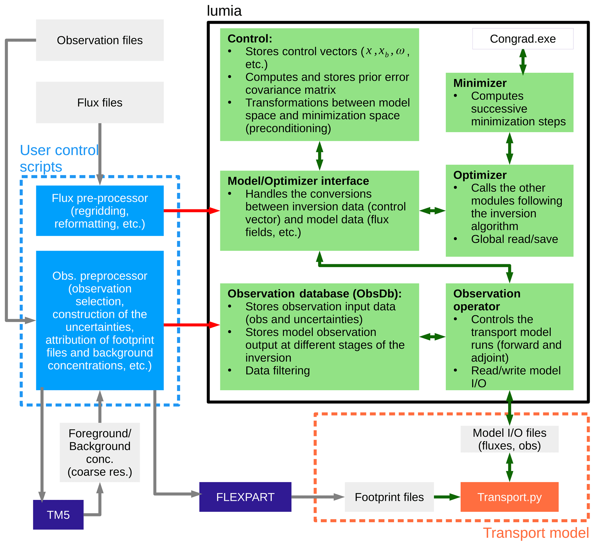
Figure 1 Inversion flow diagram. The green boxes represent code that is part of the lumia Python module; the orange box shows operations performed by the atmospheric transport model (in our case a simple Python script that reads in observations, fluxes and footprints, but a full transport model could be plugged in instead); the blue boxes show code that is typically user- and application-specific (pre-processing of data and main inversion control script). The boxes in grey mark on-disk data, and the boxes in purple show external executables

2.2 The lumia Python package

The LUMIA system is designed with the aim to provide the modularity needed to quantify the impact of the inversion design choices on the inversion results themselves. The strict isolation of the transport model also enables the transport model and the inversion algorithm to evolve independently. Unfortunately, the modularity tends to lead to an increase in the overall complexity of the code (due to the need to develop and maintain generic interfaces), which can end up being counterproductive if it limits the performances and/or usability of the system. We nonetheless believe that the benefit of a higher modularity outweighs the risks. The potential adverse effects can be mitigated by careful design choices. The code is distributed as a single Python package with the following structure (see also Fig. 1).

• The lumia folder contains the lumia Python library, which implements the basic components of the inversion such as data storage (control vector, fluxes, observations, uncertainty matrices) and functions (forward and adjoint transport, conversion functions between fluxes and control vector, cost function evaluation, etc.).

• The transport folder contains the transport Python module, which was used to implement the TM5–FLEXPART transport model coupling and is described further in Sect. 3.3.

• The src folder contains the FORTRAN source code for the conjugate gradient minimizer used in the example inversions (see Sect. 3). Replacing this external code by a native Python equivalent is planned.

• The doc folder contains documentation, mainly in the form of Jupyter notebooks, and example data and configuration files.

• The GMDD folder contains the scripts and configuration files used to produce the results presented further on in this paper.

The package can be installed using the standard “pip” command that installs lumia and transport as Python modules, which can then be imported from any Python script. The lumia module itself has a relatively flat hierarchy, which limits the risk that replacing or changing one component prevents the others from working. The implementation of alternative features is preferably carried out via the development of alternative classes, which allows each individual class to remain compact and easy to understand and maintain.

The lumia and transport modules and their submodules can be used totally independently from the inversion scripts that are provided in the GMDD folder. This allows their use in different contexts, such as development and pre- and post-processing of the inversion data or during the analysis of the results (eventually this will help to keep the inversion scripts compact, as they need only to focus on the inversion itself). The scope of the lumia library is intentionally vague: it should permit the easy construction of inversion experiments and is primarily designed for it, but our current design choices should not over-constrain the alternative use cases (such as forward transport model experiments or optimization of land surface model parameters).

3 Test inversion setup

Our test inversion setup is designed to optimize the monthly net atmosphere–ecosystem carbon flux (NEE, net ecosystem exchange) over Europe at a target horizontal resolution of 0.5^∘ using CO₂ observations from the European ICOS network (or similar and/or precursor sites). Two series of inversions are presented: first, a series of observing system synthetic experiments (OSSEs) using known truth and synthetic observations, then a series of inversions constrained by real observations. All the inversions are performed on a domain ranging from 15^∘ W, 33^∘ N to 35^∘ E, 73^∘ N (illustrated in Fig. 2) and cover the year 2011.

The inversions are performed using a variational approach, which is presented in Sect. 3.1, with a regional transport model (Sect. 3.3) that accounts for the impact of regional CO₂ fluxes from four process categories (Sect. 3.5). Section 3.4 and 3.5 present the fluxes and observations used in the inversions.

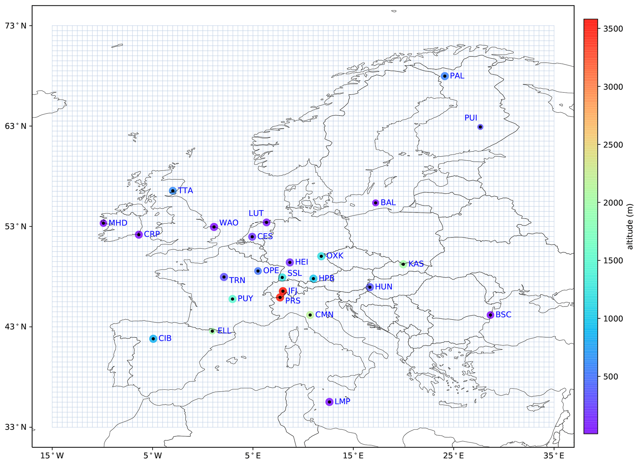
Figure 2 Regional inversion domain and location of the observation sites. The area of the dots is proportional to the number of observations available at each site (the actual number of observations is reduced by the filtering described in Sect. 3.4.4), and their color represents the altitude of the sites.

3.1 Inversion approach

We use a Bayesian variational inversion algorithm, similar to that used in TM5-4DVAR inversions (Basu et al., 2013; Meirink et al., 2008). In a variational inversion, the minimum of the cost function J(x) (Eq. 2) is solved for iteratively.

1. An initial “prior” run is performed to compute the concentrations (y_m=Hx_b) corresponding to the prior control vector x_b.

2. The local cost function (J(x=x_b)) and cost function gradient (∇_xJ(x=x_b)) are computed.

3. A control vector increment (δx) is deduced from the gradient, and the process is repeated from step 1 (with $\mathit{x}={\mathit{x}}_b+\mathit{\delta }\mathit{x}$) until a convergence criterion is reached.

The control vector increments are computed using an external library implementing the Lanczos algorithm (Lanczos, 1950). For efficiency (reduction of the number of iterations) and practicality (reduction of the number of large matrix multiplications) reasons, the optimization is performed on the preconditioned variable $\mathit{\omega }={\mathbf{B}}^{-\mathrm{1}/\mathrm{2}}(\mathit{x}-{\mathit{x}}_b)$ (following Courtier et al., 1994, and similar to the implementation in Basu et al., 2013). Equation (2) then becomes

$$\begin{array}{}\text{(3)}& J\left(\mathit{\omega }\right)={\displaystyle \frac{\mathrm{1}}{\mathrm{2}}}{\mathit{\omega }}^T\mathit{\omega }+{\displaystyle \frac{\mathrm{1}}{\mathrm{2}}}{\left({\mathbf{HB}}^{\mathrm{1}/\mathrm{2}}\mathit{\omega }+{\mathit{d}}_{\mathrm{0}}\right)}^T{\mathbf{R}}^{-\mathrm{1}}\left({\mathbf{HB}}^{\mathrm{1}/\mathrm{2}}\mathit{\omega }+{\mathit{d}}_{\mathrm{0}}\right),\end{array}$$

with ${\mathit{d}}_{\mathrm{0}}=\mathbf{H}{\mathit{x}}_b-\mathit{y}$ representing the prior model–data mismatches. In this formulation, the cost function gradient is given by

$$\begin{array}{}\text{(4)}& \begin{array}{rl}{\mathrm{\nabla }}_{\mathit{\omega }}J& =\mathit{\omega }+{\mathbf{B}}^{T/\mathrm{2}}{\mathbf{H}}^T{\mathbf{R}}^{-\mathrm{1}}\left(\mathbf{H}\mathit{x}-\mathit{y}\right)\\ & =\mathit{\omega }+{\mathbf{B}}^{T/\mathrm{2}}{\mathrm{\nabla }}_{\mathit{x}}{J}_{\text{obs}}.\end{array}\end{array}$$

The non-preconditioned observational cost function gradient ${\mathrm{\nabla }}_x{J}_{\text{obs}}={\mathbf{H}}^T{\mathbf{R}}^{-\mathrm{1}}\left(\mathbf{H}\mathit{x}-\mathit{y}\right)$ is computed using the adjoint technique (Errico, 1997). The transformation matrix ${\mathbf{B}}^{\mathrm{1}/\mathrm{2}}$ is obtained by eigenvalue decomposition of B. Note that in this formulation, the inverse of B (or the square root of its inverse) is actually never needed, making it possible to constrain the inversion with a non-invertible matrix. In practice, the preconditioning adds two extra steps to the algorithm described above: conversion from ω to x ($\mathit{x}={\mathbf{B}}^{\mathrm{1}/\mathrm{2}}\mathit{\omega }+{\mathit{x}}_b$) before applying the transport operator (i.e., running the transport model) just before step 1 and conversion from ∇_xJ_obs to ∇_ωJ_obs (just after step 2). The initial preconditioned control vector ω is filled with zeros and corresponds to x₀=x_b.

3.2 Control vector

The observation operator (H in Eq. 2) groups the ensemble of operations to compute the CO₂ concentrations corresponding to a given control vector. It includes the transport model (and its adjoint), but also the steps required to generate transport model parameters based on a given control vector. Indeed, inversions generally do not directly adjust the transport model parameters but a subset or a construct of them: inversions are generally performed at a lower temporal and/or spatial resolution than the transport, and some of the transport model parameters may be prescribed, such as fluxes from processes that are better known. The inversions performed here optimize a monthly offset to the NEE at the spatial resolution of the regional transport model: the prior control vector slice x_b(m) containing the gridded offset for the month m is defined as

$$\begin{array}{}\text{(5)}& {\mathit{x}}_b\left(m\right)=\sum _t{\mathit{f}}_{{\mathrm{0}}_m}^{\text{nee}}\left(t\right),\end{array}$$

with ${\mathit{f}}_{{\mathrm{0}}_m}^{\text{nee}}$ representing the prior 3-hourly NEE for the month m.

The reverse operation, i.e., the construction of a 3-hourly NEE field based on a given control vector x, is given by

$$\begin{array}{}\text{(6)}& {\mathit{f}}_m^{\text{nee}}={\displaystyle \frac{{\mathit{x}}^m-{\mathit{x}}_b^m}{n_t}}+{\mathit{f}}_{{\mathrm{0}}_{m,\text{nee}}}^t,\end{array}$$

with n_t representing the number of 3-hourly time intervals in that month m.

Prescribed CO₂ fluxes (anthropogenic, ocean, biomass burning) are stored in memory throughout the inversion and used at each iteration, along with the updated NEE estimate, to generate a new transport model input file.

The adjoint operation corresponding to Eq. (6) is simply

$$\begin{array}{}\text{(7)}& {\mathit{x}}_{\text{adj}}\left(m\right)={\displaystyle \frac{\mathrm{1}}{n_t}}\sum _{t=\mathrm{1}}^{n_t}{\mathit{f}}_{{\text{adj}}_m}^{\text{nee}}\left(t\right),\end{array}$$

where ${\mathit{f}}_{\text{adj}}^{\text{nee}}$ is the adjoint NEE flux (computed by the adjoint transport model described in the next section). Since only the NEE is optimized, the adjoint is zero for the other flux categories.

The adjustment of an offset to the 3-hourly NEE ensures that the amplitude of the daily cycle of NEE remains realistic. This definition of the control vector is in some respects sub-optimal: in particular, the control vector is un-necessarily large as it contains pixels for which NEE is by definition always zero, e.g., in the ocean. However, the aim here was not to obtain the best-performing inversion, but a setup easy to develop, test and replicate that will serve as a basis of comparison in future evolutions of the setup. It is, however, already possible to run LUMIA inversions with more complex configurations, such as variable spatial and temporal resolutions.

3.3 Transport model: TM5–FLEXPART coupling

For this first implementation of CO₂ inversions with LUMIA, we opted for a regional transport model based on an offline coupling of the TM5 and FLEXPART transport models, following the coupling approach proposed by Rödenbeck et al. (2009). We provide sufficient information here to replicate our setup, but refer to Rödenbeck et al. (2009) for more complete details on the coupling approach.

For each observation i, the CO₂ concentration $y_m^i$ is defined as the sum of “foreground” (near-field) and “background” (far-field) contributions.

$$\begin{array}{}\text{(8)}& y_m^i=y_{\text{bg}}^i+y_{\text{fg}}^i\end{array}$$

We used the global coarse-resolution TM5-4DVAR inversion system to compute the background component of the concentrations. The TM5 setup is described in further detail in Sect. 3.3.2. For the foreground part, we used pre-computed observation footprints computed with the FLEXPART Lagrangian transport model (Sect. 3.3.1):

$$\begin{array}{}\text{(9)}& y_m^i=y_{\text{bg}}^i+\sum _i\sum _c\langle {\mathit{K}}_i,{\mathit{f}}_c\rangle ,\end{array}$$

where the footprint K_i is a vector that stores the sensitivity of the observation yⁱ to the surface fluxes f_c such that ${\forall }_{{\mathit{f}}_c},\langle {\mathit{K}}_i,\mathit{f}\rangle =K_i\left({\mathit{f}}_c\right)$, with K being the transport model used to compute the footprint K. The footprints and the fluxes are defined on a half-degree, 3-hourly grid, and the fluxes are defined in four categories (NEE, anthropogenic, ocean and biomass burning), which is described further in Sect. 3.5. The fluxes are provided in units of µ mol (CO₂) m⁻² s⁻¹ and the footprints are in s m⁻² mol (air)⁻¹. The transport model makes no specific distinction between optimized and prescribed fluxes.

The adjoint of the operation represented by Eq. (9) is

$$\begin{array}{}\text{(10)}& {\mathit{f}}_{\text{adj}}^{\text{nee}}=\sum _i{\mathit{K}}_i^t\mathit{\delta }{y}^i,\end{array}$$

with ${\mathit{\delta }}_y^i$ being the model–data mismatches weighted by their uncertainties (Sect. 3.4.1). The adjoint flux field f_adj is calculated only for the flux categories optimized by the inversion (i.e., NEE).

The forward and adjoint transport applications (i.e., Eqs. 9 and 10) are handled by a separate Python executable called as a subprocess, which acts as a “pseudo-transport model” in our inversions. It uses FLEXPART footprints and TM5 background concentrations as input data: neither of the two transport models is directly called during the inversion, and the footprints and backgrounds can in principle be computed using different transport models or even different methods than those described in Sect. 3.3.2 and 3.3.1.

Using pre-computed footprints greatly reduces the computational cost of the inversions, since the forward and adjoint transport model applications simply consist of a series of very simple array operations. This is, however, at the cost of an increase in I/O and storage requirements (one footprint K must be stored for each observation and is read in at each forward and adjoint iteration). The isolation of the pseudo-transport model in a separate executable was not necessary from a technical point of view, but it makes its replacement by a full transport model (e.g., an Eulerian model) easier.

3.3.1 Observation footprints (FLEXPART)

The footprints (K) were computed using the FLEXPART 10.0 Lagrangian transport model (Seibert and Frank, 2004; Stohl et al., 2010). FLEXPART simulates the dispersion, backwards in time from the observation location, of a large number of virtual air “particles”. The footprint ${\mathit{K}}_i^{\mathit{\varphi }}$ corresponds to the aggregated residence time of the particles released for observation yⁱ in a given space–time grid box ϕ of the regional inversion and below a threshold altitude layer arbitrarily set to 100 m.

The simulations were driven by the European Centre for Medium-Range Weather Forecasts (ECMWF) ERA-Interim reanalysis extracted at a 3-hourly temporal resolution at a $\mathrm{0.5}{}^{\circ }\times \mathrm{0.5}{}^{\circ }$ horizontal resolution on a regional domain ranging from 25^∘ W, 23^∘ N to 45^∘ W, 83^∘ N, which is slightly larger than the inversion grid (in FLEXPART, the output grid, on which the footprints are generated, may be different from the grid of the input meteorological data).

One set of 3-hourly footprints was computed for each observation up to 7 d backward in time (less if all the particles leave the domain sooner). For plain or low-altitude sites (see Table 1), the particles were released from the sampling height above ground of the observations. For high-altitude sites (around which the orography is unlikely to be correctly accounted for), the particles were released from the altitude above sea level of the observation sites.

The footprints are stored in HDF5 files, following a format described in the Supplement.

3.3.2 Background concentrations (TM5)

The background CO₂ concentrations (y^bg in Eq. 9) result from the transport of CO₂-loaded air masses from outside the regional inversion domain towards the observation sites. The most straightforward approach to estimate this background influence would be to use a global, coarse-resolution, inversion-optimized CO₂ field as a boundary condition and then to transport that boundary condition towards the observation sites using the regional model. However, the risk is that the regional model transports the boundary condition slightly differently than how the global transport model would have done it, which would lead to systematic biases at the observation sites.

An alternative coupling strategy has been proposed by Rödenbeck et al. (2009). Instead of using the regional model to transport the boundary condition, it is the global model from which this boundary condition is extracted that transports it directly to the observation sites. Rödenbeck et al. (2009) used the global transport model TM3 for this, and we replicated their approach with the global TM5 transport model (Huijnen et al., 2010). The approach consists of the following steps.

1. A global coarse-resolution inversion is performed (with TM5 in our case), constrained by a set of prior CO₂ fluxes $f_{\text{apri}}^{\text{glo}}$ and by a set of surface CO₂ observations including both observations outside and inside the regional domain of the LUMIA inversion. The objective of this step is to obtain a set of optimized CO₂ fluxes $f_{\text{opt}}^{\text{glo}}$ that leads to a very realistic atmospheric CO₂ distribution in and around the regional domain. The accuracy of the fluxes themselves has less importance.

2. A forward run of TM5 is then used to calculate the CO₂ concentrations y_TM5 corresponding the fluxes $f_{\text{opt}}^{\text{glo}}$ at all the observation sites within the regional domain.

3. Another forward run of TM5 is used to calculate the foreground concentrations $y_{\text{TM5}}^{\text{fg}}$, which correspond to the part of y_TM5 that can result from the portion of the fluxes $f_{\text{opt}}^{\text{glo}}$ that is within the regional domain. These foreground concentrations are calculated using a modified forward TM5 run in which (1) the fluxes are the same as f^glo within the regional domain and zero outside, and (2) the CO₂ concentrations are reset to zero at all time steps everywhere outside the regional domain.

4. The background CO₂ concentrations are then given by $y^{\text{bg}}=y_{\text{TM5}}-y_{\text{TM5}}^{\text{fg}}$.

Note that here $y_{\text{TM5}}^{\text{fg}}$ corresponds well to the definition of the foreground concentrations given in Sect. 3.3: it accounts for the influence of the regional fluxes only as long as the air masses remain within the regional domain. As soon as they leave it, their concentration is reset to zero in the foreground TM5 run. By deduction, this impact of the regional fluxes on the boundary condition is therefore preserved in y^bg.

The initial global inversion (step 1) was performed using the TM5-4DVAR inversion system (Basu et al., 2013). The TM5 inversions were carried out at a horizontal resolution of $\mathrm{6}{}^{\circ }\times \mathrm{4}{}^{\circ }$ (longitude × latitude) with 25 hybrid sigma-pressure levels in the vertical and driven by meteorological fields from the European Centre for Medium-Range Weather Forecasts (ECMWF) ERA-Interim reanalysis project (Dee et al., 2011). The NEE was optimized in TM5 on a monthly global $\mathrm{6}{}^{\circ }\times \mathrm{4}{}^{\circ }$ grid, and three additional prescribed CO₂ flux categories were transported (fossil fuel, biomass burning and ocean sink). It was constrained by flask observations from the NOAA ESRL Carbon Cycle Cooperative Global Air Sampling Network (Dlugokencky et al., 2019) outside the European domain and by a subset of the observations used for the regional inversion within the European domain (see Sect. 3.4 for references and Table SI1 for a full list of the sites used in that step). For sites with continuous data (i.e., within Europe), the same data filtering as in the LUMIA inversions was used (Sect. 3.4.4).

The TM5 inversion covers the entire period of the LUMIA inversion, plus 6 extra months at the beginning and 1 month at the end to limit the influence of the initial condition and to ensure that the background concentrations in the last month of the LUMIA inversion are well constrained by the observations (observations provide important constraints on the fluxes from the preceding month).

Since the focus of the TM5 inversion was only to produce a set of CO₂ fluxes ($f_{\text{opt}}^{\text{glo}}$) that, in step 2, would lead to a realistic global CO₂ distribution, the choice of a prior matters a lot less than the selection of observations. For practical reasons, prior fluxes from the CarbonTracker 2016 release were used (Peters et al., 2007): the NEE prior was generated by the CASA model (Potter et al., 1993); fossil fuel emissions were spatially distributed according to the EDGAR4.2 inventory (https://edgar.jrc.ec.europa.eu, last access: April 2021); biomass burning emissions are based on the GFED4.1s product (van Der Werf et al., 2017); and the ocean flux is based on the Takahashi et al. (2009) climatology. We refer to the official CarbonTracker 2016 website (https://www.esrl.noaa.gov/gmd/ccgg/carbontracker/CT2016, last access: April 2021) and to references therein for further documentation on these priors.

The total (y_TM5) and foreground ($y_{\text{TM5}}^{\text{fg}}$) CO₂ concentrations were saved continuously (every 30 min) at the coordinates of each of the observation sites used in the LUMIA inversion. The concentrations were sampled at the altitude (above sea level) of the observation sites, but also as vertical profiles between the surface (as defined in the TM5 orography) and 5000 m a.s.l. (with a vertical resolution of 250 m), which were used to construct some of the observation uncertainties.

3.4 Observations and observational uncertainties

Observations from the GLOBALVIEWplus 4.2 obspack product were used in the inversions (Cooperative Global Atmospheric Data Integration Project, 2017). For the year 2011, the product includes observations from 26 sites within our regional domain (in addition to observations from mobile platforms, which were not used). Continuous observations are available at 18 of these 26 sites, and 9 sites are at high altitude. Most of these observation sites are now part of the European ICOS network. A list of the sites (coordinates, observation frequency, sampling height and data provider) is provided in Table 1, and the location of the observations is also reported in Fig. 2.

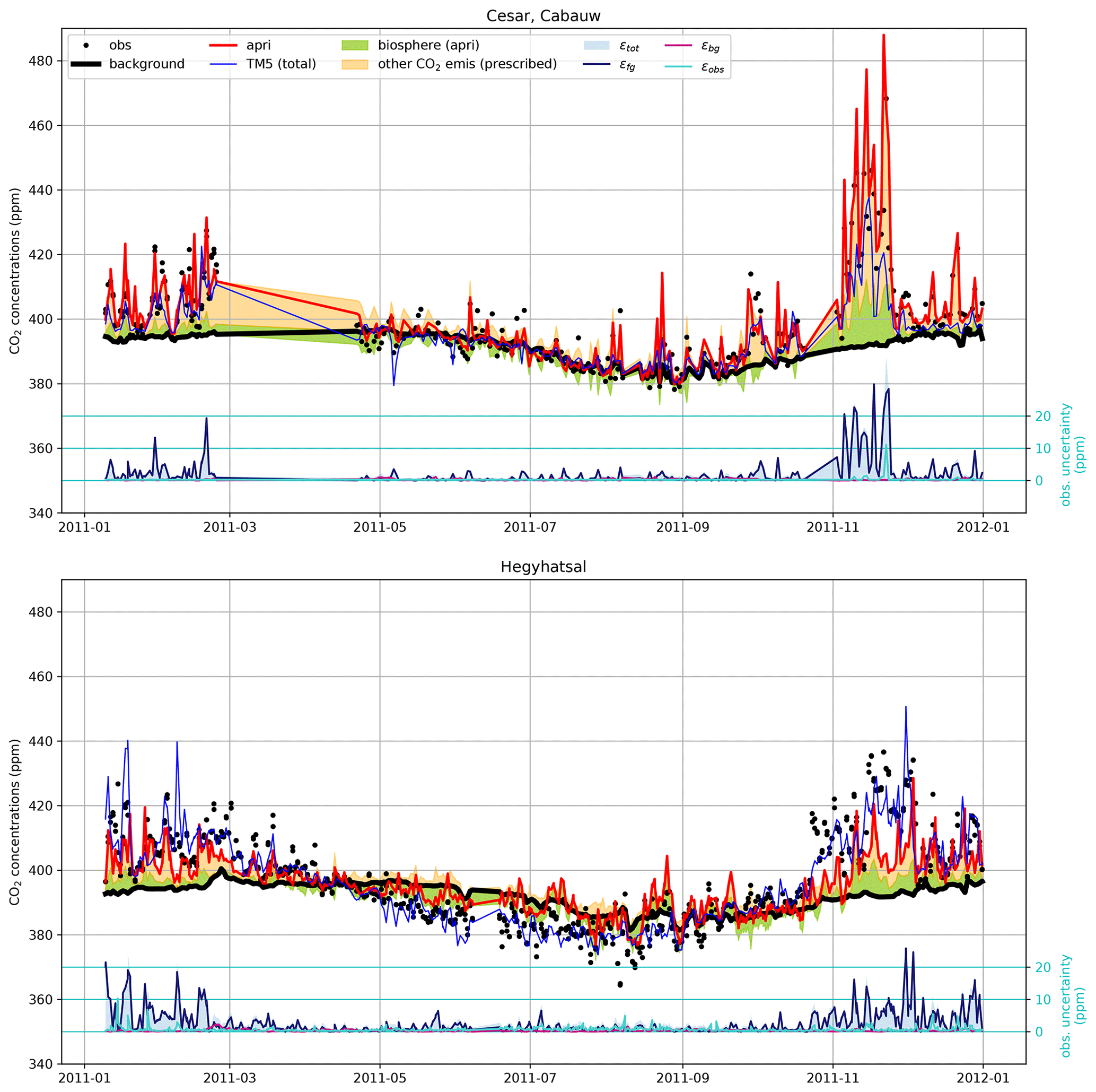
Figure 3 Decomposition of the modeled mixing ratio and of the observation uncertainties at two sites (Cabauw, the Netherlands, and Hegyhatsal, Hungary). The “TM5 total” line is the concentration computed in the coarse-resolution TM5 inversion from which the background (thick black line) is extracted. The LUMIA prior concentration is shown in red, and the green and orange shaded areas respectively show the contribution of the prior biosphere flux and of the other CO₂ fluxes to the difference between that prior and the background. The lower series of lines in each plot (with y axis on the right) show the total observation uncertainty (blue shaded area) and the contributions of the foreground, background and observational uncertainties.

3.4.1 Observation uncertainties

The observation uncertainty matrix (R) accounts for both the measurement uncertainties (ϵ_obs) and the model representation uncertainty (ϵ_H, i.e., the incapacity of the model to represent the observations perfectly well, even given perfect fluxes). In theory, the diagonal of the matrix stores the absolute total uncertainty associated with each observation, while the off-diagonals should store the observation error correlations. In practice, these correlations are difficult to quantify, and the size of the matrix would make it impractical to invert. The off-diagonals are therefore ignored in our system (as in most similar inversion setups), and the observation uncertainty is stored in a simpler observation error vector, ϵ_y.

Our inversion system uses an observation operator that decomposes the background and foreground components of the CO₂ mixing ratio; therefore, the model uncertainty itself can be decomposed into foreground and background uncertainties.

$$\begin{array}{}\text{(11)}& {\mathit{ϵ}}_y=\sqrt{max\mathit{\{}{\mathit{ϵ}}_{\text{obs}},{\mathit{ϵ}}_{\text{obs}}^{\text{min}}{\mathit{\}}}^{\mathrm{2}}+{\mathit{ϵ}}_{\text{bg}}^{\mathrm{2}}+{\mathit{ϵ}}_{\text{fg}}^{\mathrm{2}}}\end{array}$$

The instrumental error (ϵ_y) is given by the data providers for most of the observations and typically ranges 0.1–0.7 ppm (see Fig. 3). We enforced a minimum instrumental error (${\mathit{ϵ}}_{\text{obs}}^{\text{min}}$) of 0.3 ppm for all the observations.

The model representation error cannot be formally quantified, as this would require precisely knowing the CO₂ fluxes that the inversion is attempting to estimate. One can, however, assign representation error estimates (foreground and background) based, in particular, on assumptions of situations that would normally lead to a degradation of the model performances (for instance, late-night and early-morning observations, with a development of the boundary layer that may not be well captured by the model, or observations in regions with a complex orography). Transport model comparisons can also provide representation error estimates based on the difference in their results.

3.4.2 Foreground model uncertainties

As described in Sect. 3.3.2, the TM5 simulation used for computing background CO₂ concentrations also computes the foreground concentrations at each observation site. We performed a forward transport simulation with the regional transport model in LUMIA using both the background concentrations and the foreground fluxes from that TM5 simulation so that the two simulations differ only by their regional transport model. A comparison between the concentrations computed by the two models is shown in Fig. 4. The bias between the two models is very small during the summer months (it is below 0.2 ppm from April to September and goes as low as 0.01 ppm in July) but rises during the winter months (up to 1.45 ppm in November). The mean average difference between the two simulations is also much larger in winter: it ranges from 0.82 ppm in September to 4.3 ppm in November, with a yearly average of 3.3 ppm.

This comparison is not a formal performance assessment of either TM5 or of the FLEXPART-based transport used in LUMIA, and in particular the bias should be interpreted with care as the sign of the total net foreground flux changes during the year (which mechanically leads to a change of the sign of the bias). Nonetheless, it provides an indication of the order of magnitude of the foreground model transport errors. We use the absolute differences between the two models as a proxy for ϵ_fg.

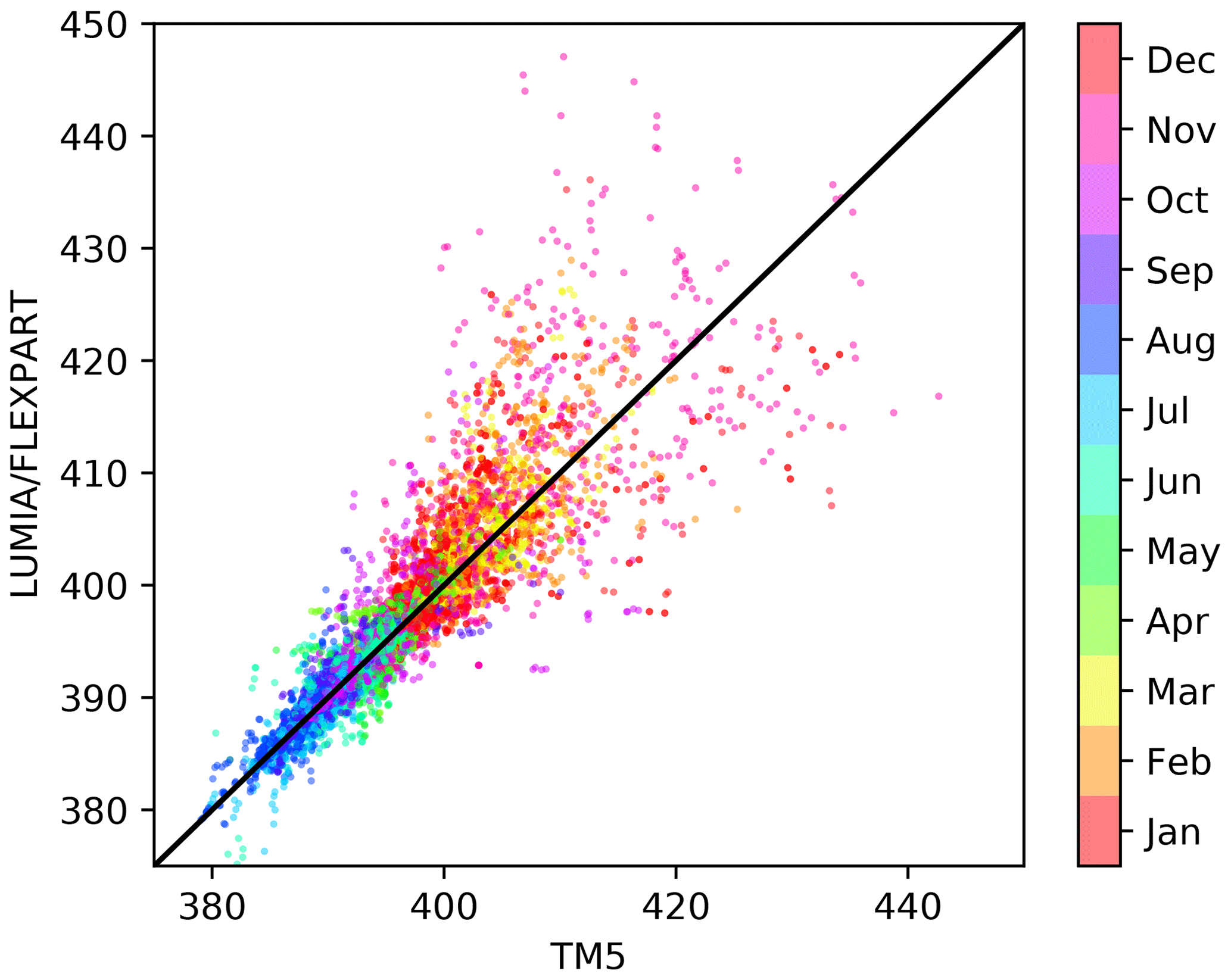
Figure 4 LUMIA CO₂ concentrations obtained from TM5–FLEXPART vs. from TM5 with the CO₂ fluxes used as the prior of the TM5 inversion (background). The color of the dots shows the observation month.

3.4.3 Background model uncertainties

Background concentrations are expected to be accurately estimated by the global TM5 inversion when the dominant winds are from the west and any signal from a strong point CO₂ source or sink has had time to dissipate along the air mass trajectory over the Atlantic Ocean. In less favorable conditions, there can be entries of less well-mixed air inside the domain, in particular in the case of easterly winds or in the event of re-entry of continental air that would have previously left the domain. These events are less likely to be well captured by the TM5 inversion and should be attributed a higher uncertainty.

There is no perfect and easy way to detect these events, but one of their consequences would be a less homogeneous background CO₂ distribution around the observation sites when they occur. As part of the TM5 simulation, vertical profiles of background concentrations were stored for each observation (from the surface to 5000 m a.s.l. at a 250 m vertical resolution). We set the background uncertainty of each observation (ϵ_bg) to the standard deviation of its corresponding background CO₂ vertical profile. ϵ_bg is on average 0.36 ppm, which is 1 order of magnitude lower than ϵ_fg, and it is also more constant (it ranges between 0.01 and 3.6 ppm). Note that these statistics are computed before the observation selection procedure described in the following section. The different components of the observation uncertainty are compared in Fig. 3 for two representative sites.

3.4.4 Observation selection

The inversions are performed on a subset of the observations included in the obspack product. Only observations for which the transport model simulation is expected to result in accurate concentrations are kept. In practice, one of the main difficulties of transport modeling is to correctly compute the mixing of air in the lower troposphere below the boundary layer. The lowest model representation error is expected for observations that are either within the boundary layer when it is most developed (in the afternoon) or well above the boundary layer for high-altitude sites (during the night). For each site with continuous observations, we selected only observations sampled during the time range for which the model is expected to perform the best. The time ranges are based on the dataset_time_window_utc flag in the metadata of the observation files from the obspack. For sites with discrete sampling, all observations were used.

Table 1 Observation sites used in the inversions. The “sets” column refers to the site selection applied in inversions SA/SP and RA/RP; set P includes only low-altitude sites and set A includes mostly high-altitude sites. Data providers are as follows. 1: Cooperative Global Atmospheric Data Integration Project (2017); 2: Vermeulen et al. (2011); 3: Ciattaglia et al. (1987); 4: David Dodd (EPA Ireland); 5: Josep Anton Morguí and Roger Curcoll (ICTA-UAB, Spain); 6: Hammer et al. (2008); 7: Haszpra et al. (2001); 8: Uglietti et al. (2011); 9: Rozanski et al. (2014); 10: Alcide Giorgio di Sarra (ENEA, Italy); 11: van der Laan et al. (2009); 12: Yver et al. (2011); 13: Hatakka et al. (2003); 14: Francesco Apadula (RSE, Italy); 15: Schmidt (2003); 16: Ganesan et al. (2015); 17: Wilson (2012); 18: Karin Uhse (UBA, Germany).

3.5 Prior and prescribed fluxes

In addition to the net ecosystem exchange (NEE, net atmosphere–land CO₂ flux) that is optimized in the inversions, the transport model also accounts for anthropogenic CO₂ emissions (combustion of fossil fuels, biofuels and cement production), biomass burning emissions (large-scale forest fires) and ocean–atmosphere CO₂ exchanges.

The NEE prior is taken from simulations of the LPJ-GUESS and ORCHIDEE vegetation models: in the OSSEs (Sect. 4) ORCHIDEE fluxes are used as prior and LPJ-GUESS fluxes are used as truth, while in inversions against real data LPJ-GUESS fluxes are used as prior. Both vegetation models provide 3-hourly fluxes on a horizontal $\mathrm{0.5}{}^{\circ }\times \mathrm{0.5}{}^{\circ }$ grid.

LPJ-GUESS (Smith et al., 2014) is a dynamic global vegetation model (DGVM), which combines process-based descriptions of terrestrial ecosystem structure (vegetation composition, biomass and height) and function (energy absorption, carbon and nitrogen cycling). The vegetation is simulated as a series of replicate patches, in which individuals of each simulated plant functional type (or species) compete for the available resources of light and water, as prescribed by the climate data. The model is forced using the WFDEI meteorological dataset (Weedon et al., 2014) and produces 3-hourly output of gross and net carbon fluxes.

ORCHIDEE is a global process-based terrestrial biosphere model (initially described in Krinner et al., 2005) that computes carbon, water and energy fluxes between the land surface and the atmosphere as well as within the soil–plant continuum. The model computes the gross primary productivity (GPP) with the assimilation of carbon based on the Farquhar et al. (1980) model for C₃ plants and thus accounts for the response of vegetation growth to increasing atmospheric CO₂ levels and to climate variability. The land cover change (including deforestation, regrowth and cropland dynamic) was prescribed using annual land cover maps derived from the harmonized land use dataset (Hurtt et al., 2011) combined with the ESA-CCI land cover products. The net and gross CO₂ fluxes used for this project correspond to the one provided for the Global Carbon Project intercomparison (Le Quéré et al., 2018) with a model version that was updated recently (Vuichard et al., 2019).

Fossil fuel emissions are based on a pre-release of the EDGARv4.3 inventory for the base year 2010 (Janssens-Maenhout et al., 2019). This specific dataset includes additional information on the fuel mix per emission sector and thus allows for a temporal scaling of the gridded annual emissions for the inversion year (2011) according to year-to-year changes in fuel consumption data at the national level (bp2, 2016), following the approach of Steinbach et al. (2011). A further temporal disaggregation into hourly emissions is based on specific temporal factors (seasonal, weekly and daily cycles) for different emission sectors (Denier van der Gon et al., 2011).

The ocean–atmosphere flux is taken from the Jena CarboScope v1.5 product, which provides temporally and spatially resolved estimates of the global sea–air CO₂ flux estimated by fitting a simple data-driven diagnostic model of ocean mixed-layer biogeochemistry to surface-ocean CO₂ partial pressure data from the SOCAT v1.5 database (Rödenbeck et al., 2013).

A biomass burning flux category was also included in the inversion based on fluxes from the Global Fire Emission Database v4 (Giglio et al., 2013). In our European domain biomass burning emissions are negligible compared to the other CO₂ emission sources; however, we include them for completeness.

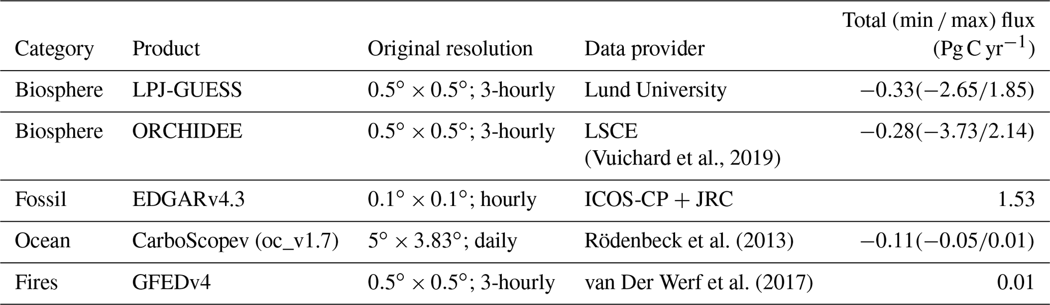
All fluxes are regridded on the same $\mathrm{0.5}{}^{\circ }\times \mathrm{0.5}{}^{\circ }$, 3-hourly resolution (by simple aggregation or re-binning). A summary of the prior fluxes sources, original resolution and yearly totals is provided in Table 2.

(Vuichard et al., 2019)Rödenbeck et al. (2013)van Der Werf et al. (2017)

Table 2 Prior and prescribed CO₂ fluxes. Min $/$ max values are provided for the fluxes that have both positive and negative components and correspond to the minimum and maximum values of the 3-hourly flux aggregated over the entire domain (Pg C yr⁻¹).

3.5.1 Prior uncertainties

The background error covariance matrix (B in Eq. 2) is constructed following the “correlation length” approach used in many other inversion systems (e.g., Houweling et al., 2014; Thompson et al., 2015; Chevallier et al., 2005): the error covariance between control vector elements x₁ and x₂ at grid cells with coordinates $p_{\mathrm{1}}=(i_{\mathrm{1}},j_{\mathrm{1}},t_{\mathrm{1}})$ and $p_{\mathrm{2}}=(i_{\mathrm{2}},j_{\mathrm{2}},t_{\mathrm{2}})$ is defined as

$$\begin{array}{}\text{(12)}& \text{cov}({\mathit{x}}_{\mathrm{1}},{\mathit{x}}_{\mathrm{2}})={\mathit{\sigma }}_{{\mathit{x}}_{\mathrm{1}}}^{\mathrm{2}}\cdot {\mathit{\sigma }}_{{\mathit{x}}_{\mathrm{2}}}^{\mathrm{2}}{e}^{-{\left(d(p_{\mathrm{1}},p_{\mathrm{2}})/L_h\right)}^{\mathrm{2}}}{e}^{-|t_{\mathrm{1}}-t_{\mathrm{2}}|/L_t},\end{array}$$

where ${\mathit{\sigma }}_{{\mathit{x}}_{\mathrm{1}}}^{\mathrm{2}}$ and ${\mathit{\sigma }}_{{\mathit{x}}_{\mathrm{2}}}^{\mathrm{2}}$ are the variances assigned to the prior monthly NEE at coordinates p₁ and p₂, and L_h and L_t are correlation lengths that define how rapidly the correlation between two components drops as a function of their distance in time and space.

The true uncertainty of the prior fluxes (${\mathit{\sigma }}_{\mathit{x}}^{\mathrm{2}}$) is difficult to evaluate and is therefore constructed on reasonable but arbitrary assumptions. We tested several approaches, which are further discussed in Sect. 4: (1) scaling the uncertainties linearly to the absolute monthly flux; (2) scaling the uncertainties to the absolute net 3-hourly flux (and then cumulating these 3-hourly uncertainties to the monthly scale); and (3) enforcing constant monthly uncertainties throughout the year at the domain scale.

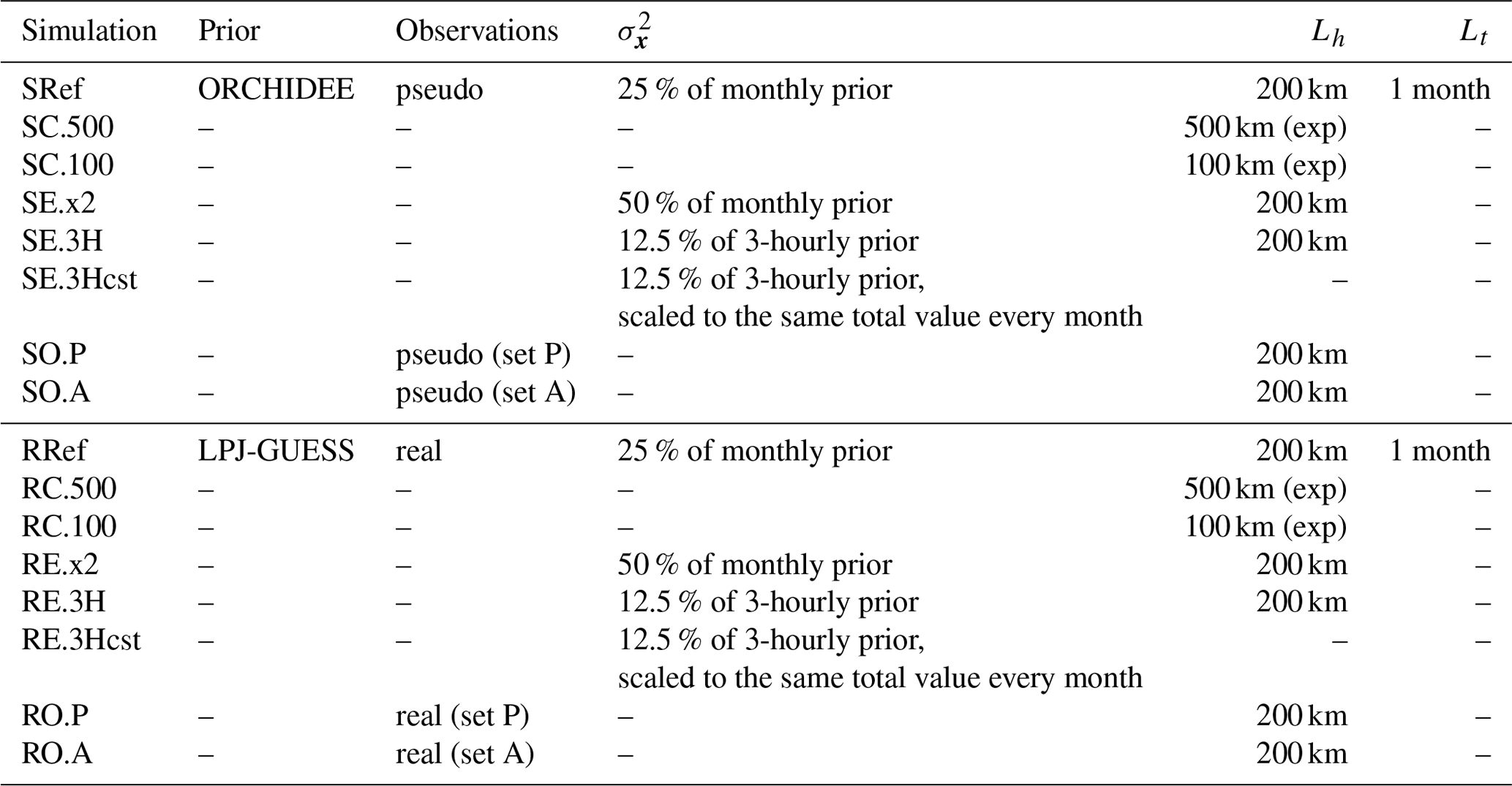
3.6 Inversions performed

We performed two sets of inversions, which are listed in Table 3. The first set consists of observing system simulation experiments (OSSEs) and is designed to assess the theoretical performance of the inversions in the absence of transport model errors. The second test consists of inversions using real observations.

In the OSSEs, the LPJ-GUESS NEE dataset was taken as an arbitrary truth, and a dataset of synthetic pseudo-observations was generated at the times and locations of the actual observations listed in Table 1 by forward propagation of the “true’’ NEE flux with the transport model (also including the contributions of non-optimized fluxes listed in Sect. 3.5). Random perturbations were then added to mimic the measurement error ($y=y^{\text{truth}}+\mathcal{N}(\mathrm{0},{\mathit{\sigma }}_y^{\mathrm{2}})$, with ${\mathit{\sigma }}_y^{\mathrm{2}}$ being the uncertainty of each observation as defined in the matrix R).

The OSSEs use this set of pseudo-observations as observational constraints and the ORCHIDEE NEE dataset as a prior. The reference OSSE, SRef, uses a prior error covariance matrix (B) constructed with prior uncertainties set to 25 % of the absolute prior value (${\mathit{\sigma }}_{{\mathit{x}}_b}^{\mathrm{2}}=\mathrm{0.25}\left|{\mathit{x}}_b\right|$) and with covariances constructed from a horizontal correlation length (L_H) of 200 km and a temporal correlation length (L_t) of 30 d. In the sensitivity tests (also listed in Table 3) we vary the correlation lengths (SC.100 and SC.500), the prescribed prior uncertainties (SE.3H, SE.3Hcst, SE.x2) and the extent of the observation network (SO.A, SO.P).

The second set is essentially identical to the OSSEs, except that it uses real observations and the LPJ-GUESS flux dataset as a prior.

Table 3 List of inversion experiments performed. The restricted observation sets A and P are reported in Table 1.

4 OSSEs

We first analyze the capacity of the reference OSSE SRef to reconstruct various characteristics of the true LPJ-GUESS NEE fluxes (monthly and annual NEE budget, aggregated at spatial scales ranging from the entire domain down to single pixels). Then we analyze the results of the other OSSEs to test how sensitive the results are to a range of reasonable assumptions in the inversion settings.

4.1 Reference inversion (SRef)

Figure 5 shows monthly and annual time series of NEE and NEE error (with respect to the prescribed truth) aggregated over the entire domain.

At the domain scale, the prior estimate for the annual NEE is very close to the “truth” (−0.28 and −0.34 Pg C yr⁻¹, respectively), but the amplitude of the seasonal cycle in the prior is more than double that of the truth, with monthly NEE ranging from +0.26 Pg C month⁻¹ in October to −0.66 Pg C month⁻¹ in June in the prior compared to +0.08 Pg C month⁻¹ (in January) to −0.29 Pg C month⁻¹ (in May) in the truth. In total, the absolute prior error slightly exceeds 3 Pg C yr⁻¹, peaks in June and July, and is the lowest in December–February.

The inversion improves the estimation of the seasonal cycle at the domain scale, with a seasonal cycle amplitude reduced to a range of −0.36 Pg C yr⁻¹ (May) to +0.16 Pg C yr⁻¹ (December), which is much closer to the truth, and the absolute error is reduced by nearly 40 % to 1.87 Pg C yr⁻¹. However, since the positive flux corrections in the summer months largely exceed the negative corrections from September to April, this results in a strong degradation of the annual European NEE estimate, with a near-balanced posterior flux of −0.05 Pg C yr⁻¹. This is largely because the prior was already a very good estimate of the annual NEE, but is somewhat counterintuitive to the assumption that a reduction of the errors would necessarily mean an improvement of the flux estimates at large spatial and temporal scales.

Figure 6 illustrates the spatial distribution of the error reduction. While the largest prior errors are found north of the Black Sea and in North Africa, the error reduction is rather homogeneous, except for North Africa, Turkey (which are not really constrained by the observation network) and some patches in western Europe (mainly in the UK, but also in Ireland, France and the Benelux) where the error actually increases. In total, these localized error enhancements amount to 0.16 Pg C yr⁻¹ (lower panel of Fig. 5). These isolated occurrences of error enhancements are not a sign of malfunction of the inversion system, but they highlight its limitations: they result from attributions of flux corrections to the incorrect grid cells, which can happen if the resolution of the inversion is not adapted to the constraints provided by the observation network (i.e., smoothing and aggregation errors, as defined in Turner and Jacob, 2015).

Although our control vector contains the flux estimates at the native spatial resolution of the transport model, the effective resolution of the inversion is further constrained by the covariances contained in the prior error covariance matrix B. Furthermore, the fluxes are only optimized monthly, while the actual prior error varies at a 3-hourly resolution. Since the network is not homogeneous, the choice of the inversion is necessarily a compromise, and we test its impact in the next section. The low temporal resolution was mostly chosen for practical reasons, as it made development and testing easier, but it corresponds to a standard practice in regional inversions, which tend to either optimize the fluxes at a low temporal resolution (Thompson and Stohl, 2014; van der Laan-Luijkx et al., 2017) or to impose a temporal covariance length on the order of 1 month (e.g., Broquet et al., 2011; Kountouris et al., 2018).

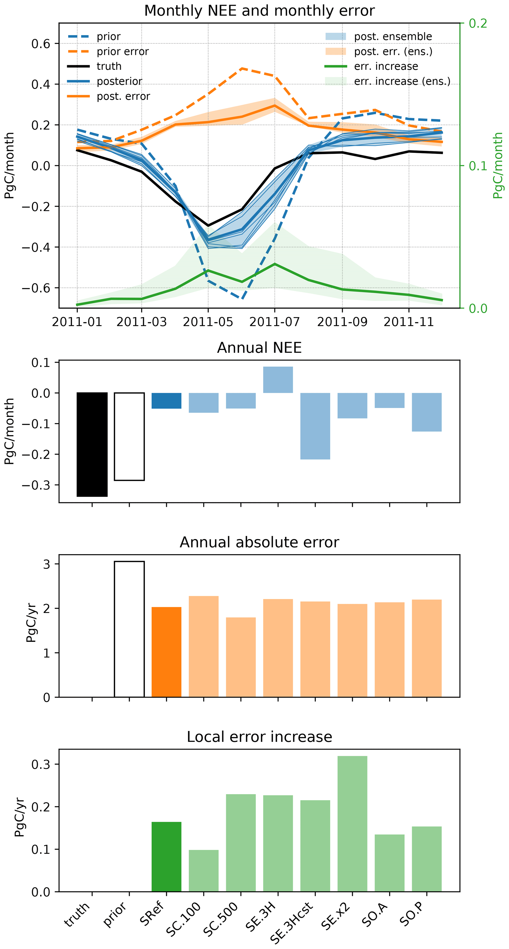
Figure 5 Upper row, left axis: monthly prior NEE (dashed blue line), true NEE (solid black line), posterior NEE (blue), absolute prior error (dashed orange line) and posterior error (orange) in the OSSEs. Upper row, right axis: total error increase (i.e., positive component of the error reduction, green). The SRef inversion is shown as solid lines, and the set of sensitivity tests is shown as a shaded area (prior and posterior ensemble). Second, third and fourth rows: same variables but aggregated annually.

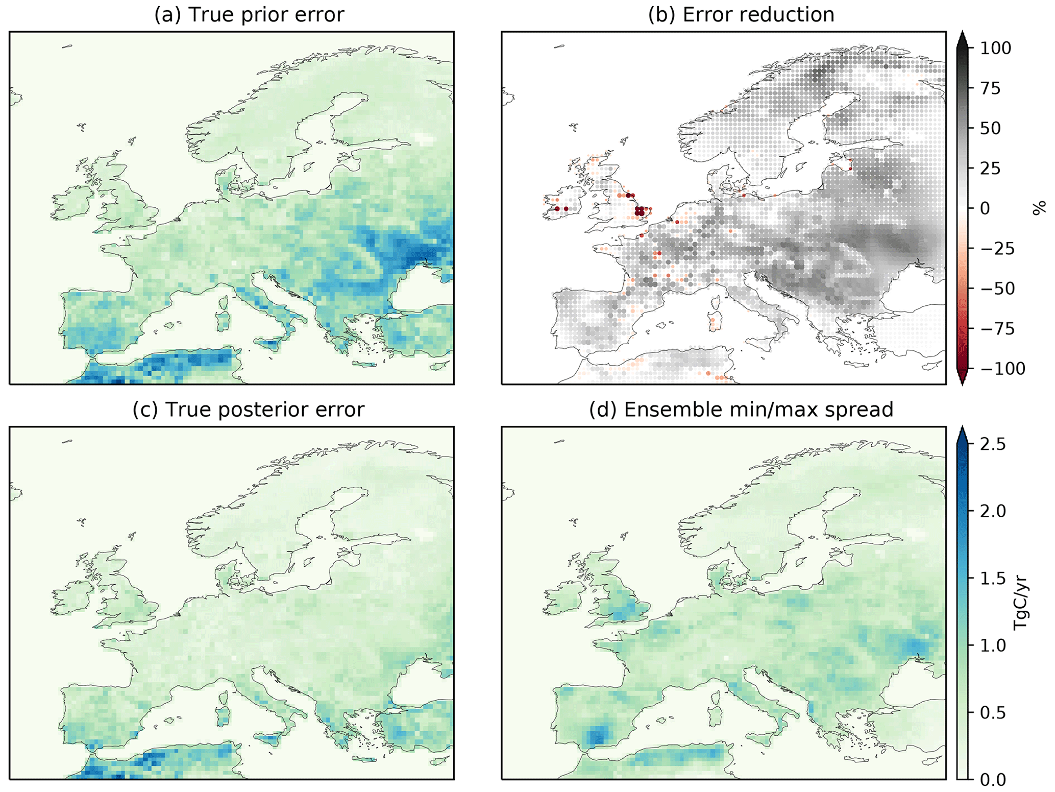
Figure 6 Prior (a) and posterior (c) total error (with respect to the prescribed truth); (b) percentage error reduction. The size of the dots is proportional to the size of the flux correction. (d) Spread of the posteriors throughout the ensemble of sensitivity tests.

4.2 Sensitivity tests

The total NEE flux, absolute error and error increase are shown in Fig. 5 for the individual sensitivity experiments at the annual scale and as an ensemble shape for the monthly scale (the monthly-scale results of the individual simulations can be found in Fig. S2).

4.2.1 Sensitivity to the error distribution

Inversions SE.3H, SE.3Hcst and SE.x2 were designed to test the impact of the prescribed prior uncertainty vector (e.g., diagonal of B) on the inversion.

• In SE.3H, the prior uncertainty is set proportional to the sum of the uncertainties in the 3-hourly fluxes: ${\mathit{\sigma }}_{{\mathit{x}}_b}=\frac{\mathrm{0.13}}{T}{\sum }_t^T\left|f_t\right|$. This avoids the situation in which GPP and respiration are significant but compensate for each other, leading to a near-zero NEE and a near-zero prior uncertainty, which can happen when the prior uncertainty is calculated following the approach used in SRef. The factor 0.13 was chosen to lead to a total annual uncertainty comparable to that of SRef. This leads to an overall redistribution of the uncertainties from the winter to the summer period, which is closer to the actual distribution of differences between the prior and truth fluxes (see Fig. S1).

• In SE.3Hcst, the prior uncertainty is computed as in SE.3H, but it is then scaled monthly so as to lead to a flat distribution of the uncertainties across the year.

• In SE.x2, the prior uncertainty is simply doubled compared to SRef.

SE.3Hcst leads to an improved value of the annual budget of NEE at the domain scale, but this is due to a poorer estimation of the summer fluxes (since the uncertainty is lower in summer, the inversion sticks more to its prior). In contrast, SE.3H leads to further degradation of the annual budget, without achieving better performances than SRef at the monthly scale. For both inversions, this translates into a slightly larger total posterior error (2.15 and 2.20 Pg C yr⁻¹, respectively, compared to 2.03 in SRef). The doubling of the prior uncertainty in SE.x2 allows it to depart more from the prior and to derive better domain-scale flux estimates both monthly and annually, but it also leads to an increase in the “added error’’ (lower panel of Fig. 5).

4.2.2 Sensitivity to the error covariance structure

Inversions SC.100 and SC.500 use prior error covariance matrices constructed using shorter (100 km) and longer (500 km) horizontal correlation lengths (L_H), respectively, than SRef. The longer covariance length in SC.500 forces the inversion to favor large-scale, low-amplitude flux corrections over localized strong adjustments. Since the prior error follows a relatively homogeneous pattern, SC.500 effectively produces a better estimation of the NEE, especially in eastern Europe where the network is sparse (Fig. S4b). The opposite happens with SC.100, which tends to concentrate the flux adjustments in the vicinity of the observation sites.

At the domain scale, the annual budgets are nearly identical in SC.100, SC.500 and SRef. However, the total error reduction is lower in SC.100 and higher in SC.500 compared to SRef (0.78, 1.28 and 1.02 Pg C yr⁻¹, respectively), but the added error is larger in SC.500 (0.23 Pg C yr⁻¹) and lower in SC.100 (0.10 Pg C yr⁻¹): this confirms the hypothesis that these are aggregation errors that can be reduced by increasing the number of degrees of freedom in the inversion (for instance, by reducing the covariance constraints).

4.2.3 Sensitivity to the observation network density

Compared to SRef, SO.A uses only high-altitude observations (plus LMP and TTA as these were the only sites available in their region) and SO.P uses only low-altitude sites. In terms of the annual budget, SO.P outperforms most of the other inversions, but as for SE.3Hcst, this results from poorer flux corrections in summer rather than from a better overall reduction of the uncertainties. In contrast, SO.A leads to results very comparable to SRef at the domain scale, with a nearly identical seasonal cycle and net annual flux. The net error reduction, however, remains slightly better in SRef (see also Fig. S1 for the seasonal cycles of SO.A and SO.P).

4.3 Evolution of the fit to the observations

The comparison of the prior and posterior model fit to observations is a classical diagnostic of atmospheric inversions (Michalak et al., 2017). The inversion is expected to improve the overall fit to the observation ensemble, and a lack of statistical improvement would generally be a sign of a malfunctioning inversion algorithm. At a finer scale, analysis of when and where the representation of the observations is most improved (or degraded) can provide useful insights on the performance of the inversion (adequacy of the definition of uncertainties) and on those of the underlying transport model.

In the right panel of Fig. 7, we compare the statistical distribution of prior and posterior observation fit residuals for inversion SRef. The plot confirms that the inversion leads to an overall improvement of the representation of observations, although it is modest (prior bias – model-obs: 0.2 ppm; posterior bias: 0.05 ppm; prior RMSE: 4.9 ppm; posterior RMSE: 3.75 ppm). The left panel shows the root mean square error (RMSE) reduction at each observation site (the size of the dots is proportional to the number of assimilated observations at each site, and the color shows the net RMSE reduction). At all sites the inversion leads to improvements in the fit, but those are generally much more modest in western Europe, which can be explained by the (coincidental) good performance of the prior in that region (see Fig. 6), but also by the strong sensitivity of these sites to background concentrations. Sites in the UK and, in particular, Ireland sample very little continental air, which leaves little margin for the inversion to improve the representation of their observations.

The center panel of Fig. 7 compares the RMSE reduction of inversion SRef to that of the other OSSEs. The best performances are logically achieved by SE.x2, which can depart much more from its prior than the other inversions. On the other hand, SC.100 systematically underperforms the ensemble, which is consistent with its poorer flux error reduction. In general, however, the reduction of misfits is very similar and is not a good indicator for the quality of the optimized fluxes.

.

Figure 7 (a) Map of the observation sites in SRef, with the area of the dots proportional to the number of assimilated observations at each site and the color proportional to the RMSE reduction (prior RMSE minus posterior RMSE). (b) RMSE reduction at each site for the five sensitivity OSSEs. (c) Distribution of observation residuals with the prior, posterior (SRef) and truth fluxes. The blues lines in the center plot show the prior (dashed line) and posterior (solid line) mean biases at each site (axis on the right)

5 Inversions with real observations

The OSSEs presented above neglect several complications of real inversions, in particular transport model errors (the observations were generated using the same transport model as the one used in the inversions). While it is not within the scope of this paper to precisely quantify these errors, we nonetheless performed a series of inversions constrained by real observations to assess to what extent the characteristics of the inversion results identified with the OSSEs remain under a more realistic situation.

The set of inversions used here is identical to the set of OSSEs, except that real observations are used and that the LPJ-GUESS flux is used as a prior (instead of ORCHIDEE in the OSSEs). The inversion settings are reported in Table 3.

5.1 Posterior fluxes

The monthly and annual prior and posterior NEEs are shown in Fig. 8 for the reference RRef inversion and for the sensitivity tests. The inversion leads to a slight increase in the seasonal cycle amplitude, with a peak summer uptake increased by 24 % in May (−0.36 Pg C month⁻¹ instead of −0.24 Pg C month⁻¹ in the prior) and a nearly doubling of the CO₂ emissions in winter (+0.12 Pg C month⁻¹ instead of +0.07 Pg C month⁻¹ in the prior in November). It also leads to a delayed date for the change of sign of the net flux in both the spring and the autumn (the net prior flux becomes negative in March in the prior and positive again in August, while it only becomes negative in April and positive in October in RRef).

These monthly flux adjustments do not result in a change in the net annual flux (−0.33 Pg C yr⁻¹ in both the prior and the RRef posterior). As seen when analyzing the OSSE results, the net annual budget is not well constrained by the inversions, and the absence of change here is purely coincidental.

In contrast to the OSSEs, the transport model error is not zero, which may explain the slightly higher sensitivity of the results to the extent of the observation network: RO.P and RO.A differ by, on average, 0.02 Pg C month⁻¹, which is double the average difference between SO.P and SO.A. However, the overall spread of results in that second set of inversions is of the same order of magnitude as that obtained with the OSSEs, with a monthly spread ranging from 0.02 Pg C month⁻¹ (January and September) to 0.07 Pg C month⁻¹ (March and August). This indicates that the conclusions of the OSSEs regarding the robustness of the results can be generalized to these inversions with real data.

Maps of the prior and posterior fluxes, as well as the flux adjustments obtained with RRef, are shown in Fig. 9 for three 4-month periods. The January to April and September to December periods approximately correspond to the time of the year when a positive NEE correction is obtained by the inversion, while May to August is the period when the inversion finds increased uptake compared to the prior. While at large scales, the inversion preserves the spatial distribution of NEE well, the flux adjustment is not as homogeneous as what was obtained with the OSSEs (see also monthly flux adjustment maps in Fig. S5b).

The ensemble variability (lower row of Fig. 9) is much higher than in the OSSEs in northwestern Europe (northern France, Ireland and the UK) and in Hungary around the Hegyhatsal observation site (see also Fig. 6). In the latter case, this is mainly due to the inclusion (or not) of this site in the inversions (i.e., RO.A/RO.P inversions). The discrepancies in northwestern Europe were already present in the OSSEs, but here with real observations the inversions additionally have to compensate for the inaccuracy of the transport model. In particular, errors in the prescribed background concentrations will have a stronger impact on the optimized fluxes in the vicinity of sites that sample predominantly background concentrations, such as the sites in Ireland and the UK. But also, observation sites downwind of large urban areas are more susceptible to impacts by errors in the prescribed fossil fuel emissions, either because the emission scenario itself is incorrect or the transport model resolution is too coarse to correctly represent the impact of these emissions at the observation site.

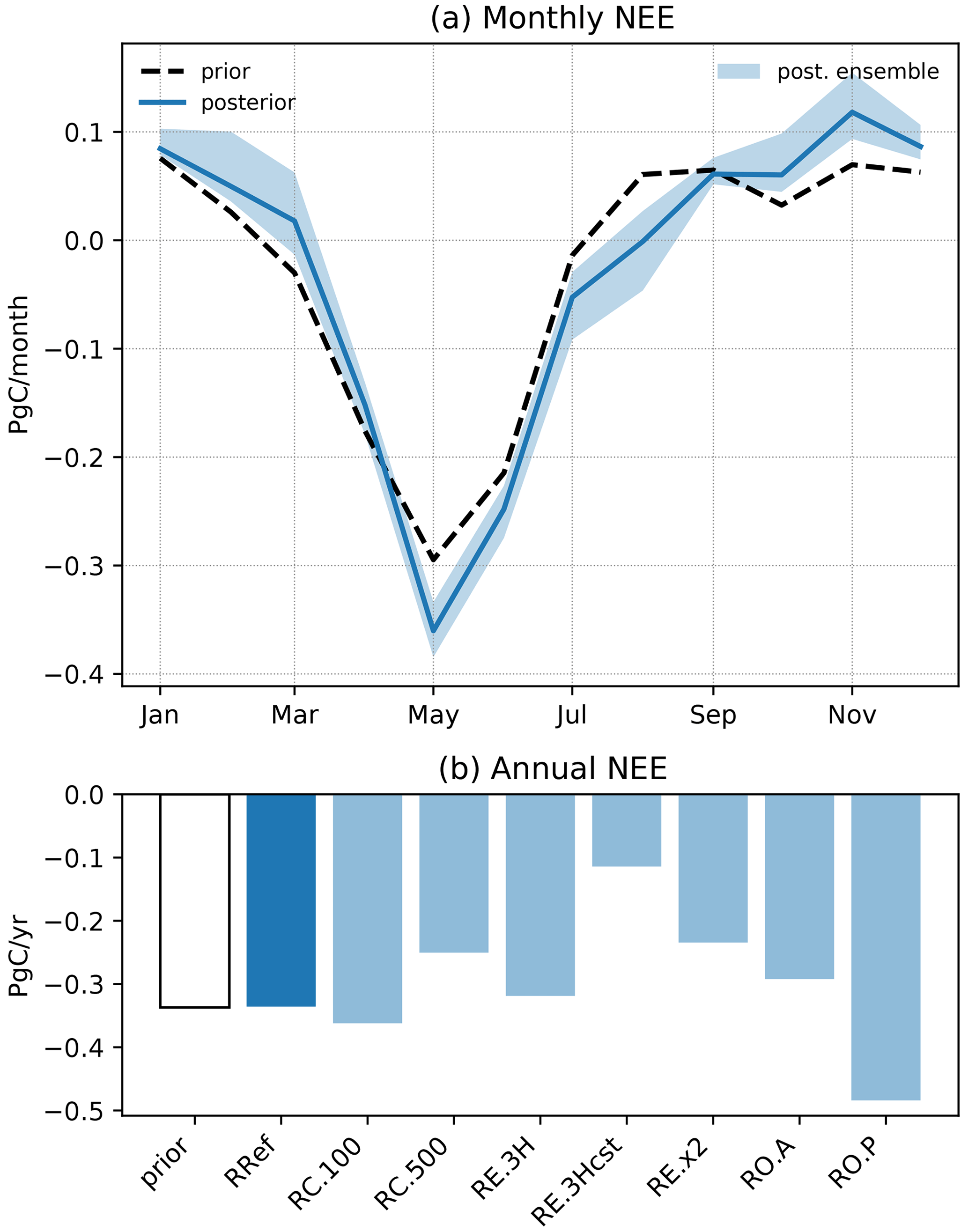
Figure 8 (a) Monthly prior (dashed black line) and posterior NEE (solid line: RRef; shaded blue area: ensemble spread); (b) annual NEE for the prior LPJ-GUESS and the seven inversion posteriors.

Figure 9 Total prior NEE (top), posterior NEE (second row) and NEE adjustment (third row) for the RRef inversion and for three 4-month periods (left to right); bottom row: posterior ensemble spread.

5.2 Reduction of the observation misfits

Figure 10 provides an overview of the model–data mismatches for RRef and, at the site level, for the sensitivity experiments. As expected, the inversion leads to a reduction in the RMSE, from 5.8 ppm in the prior to 4.8 ppm in the posterior, and to a slight reduction of the mean bias (from −0.2 to −0.1 ppm). These values are slightly larger than the ones obtained in the OSSEs, which is consistent with the presence of a non-perfect transport model and boundary conditions.

At the site level, the prior biases are more variable than in the OSSEs, from −9.1 ppm at Baltic Sea (BSC) to +2 ppm at Ochsenkopf (OXK). The bias corrections remain very modest at most sites (the bias even slightly increases at a few sites). The large (7.5 ppm) bias at BSC (Black Sea) is computed from a very small number of observations (17 in total, with observational errors up to 8 ppm), which therefore have very little weight in the inversion. The RMSE is generally reduced, except at ELL (Estany Llong, Spain) and OXK (Ochsenkopf, Germany) where the fit to the observations is slightly degraded. Both sites are located in relative proximity to other observation sites, with which their footprints overlap: the degradation of the RMSE results from contradictory constraints provided to the inversions by these different sites. The inversion does not have sufficient degrees of freedom to simultaneously improve the fit at all sites and therefore degrades the fit to the OXK and ELL observations, which have few observations (48 and 8, respectively). The problem is common to all the sensitivity runs, and the mean posterior biases are also very similar across the inversions.

As seen with the OSSEs, a better performance in the fit to observations is not necessarily an indication of a more accurate optimized solution. The site-by-site analysis of the misfits might point to limitations of the transport operator, but a more in-depth analysis would be required, which is out of the scope of this paper.

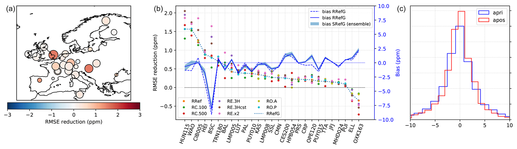
Figure 10 (a) Map of the observation sites in RRef, with the area of the dots proportional to the number of assimilated observations at each site and the color proportional to the RMSE reduction (prior RMSE minus posterior RMSE). (b) RMSE reduction at each site for the five sensitivity OSSEs, as well as prior (dashed blue line) and posterior (solid blue line) mean biases at each site (axis on the right). (c) Prior and posterior distribution of the observation mismatches in RRef (irrespective of the site).

6 Discussion and conclusions

We have set up an atmospheric inversion system based on an implementation of the variational inversion approach (Sect. 3.1) with a transport model based on an offline coupling between FLEXPART (high-resolution regional transport) and TM5 (coarse-resolution transport of the background fluxes and historical atmospheric CO₂ burden). The inversion setup was then tested through a series of synthetic experiments and realistic inversions designed to verify that the inversions work as expected and to test the sensitivity of the results to typically user-defined settings. In this section we separately discuss three aspects of the paper: first, the inversion results themselves, then the TM5–FLEXPART coupling and finally the LUMIA system.

6.1 Inversion approach and results

The inversion setup was designed to optimize European NEE at a monthly 0.5^∘ scale based on in situ observations from a tall-tower network. The setup is intentionally simple as the focus at this stage was on developing a robust technical base and having a reference setup for future projects. The transport model is a transposition to TM5 and FLEXPART of the offline coupling approach developed for TM3 and STILT by Rödenbeck et al. (2009), and the optimization itself shares many similarities with existing variational inversion systems, e.g., TM5-4DVAR (Basu et al., 2013), TM3–STILT (Kountouris et al., 2018) and PyVAR–CHIMERE (Broquet et al., 2011), which should facilitate the comparison of results with these systems. We discuss our results under the perspective of determining how capable our inversion system is at estimating some characteristics of the CO₂ fluxes and identifying directions for further improvements.

The first inversion results suggest that the inversion system is working as expected. In the OSSEs, the inversions enable on average a 40 % reduction of the monthly flux error at the grid-cell scale, and the differences between the optimized fluxes obtained from different sensitivity runs are in line with what could be expected from the different settings used. However, these local error reductions can be of opposite sign and do not always add up to a net error reduction at larger scales. In particular, while the NEE estimate is generally always improved at the monthly scale, the positive corrections in summer are much stronger than the negative corrections in winter, which results in an overall degradation of the annual NEE. Using an even month-to-month distribution of the uncertainties (SE.3Hcst inversion) leads to a more realistic annual estimate, but also to a higher occurrence of local degradations of the solution, which further complicates the interpretation of the results.

This high sensitivity of the annual NEE to the different choices of prior uncertainty show that this specific metric is not well constrained in our inversions. With further tuning, it might be possible to find a formulation of the prior uncertainties that allows OSSEs to converge towards the true annual NEE (see, e.g., Kountouris et al., 2018), but there is no guarantee that applying the same methodology in real inversions would enable a reliable determination of the true NEE, since the differences between the truth and prior in our OSSEs do not necessarily approximate the real error of the bottom-up estimates well. It may, in fact, remain very hard to estimate the annual NEE more robustly without introducing further constraints in the system. One straightforward way to do so would be to increase the density of observations: indeed, we see that the results gain consistency (i.e., become less sensitive to sensitivity experiments) where the observation network is dense, which is encouraging since the number of observation sites in Europe has significantly increased compared to the data selection used in this paper.

A complementary approach could be to make better use of constraints from observations outside the domain: by definition, they cannot be accounted for directly by the regional inversion, but they were used to constrain the global inversion from which the background concentrations were extracted. By construction, the flux estimate in that global inversion is consistent with observations downwind of Europe, which is not necessarily the case in our regional inversions (there is no constraint on the CO₂ concentration of the outgoing air and therefore on the net regional flux). One may then argue that, if the global inversion provides a more reliable CO₂ flux estimate at the continental scale, then this large-scale flux estimate could be used as an additional constraint in the regional inversion. This would clarify the respective role of the regional and global inversions: the global one would estimate the fluxes at the scale of the continent and the regional one would redistribute them at a finer scale. This, however, raises the question of the confidence level that can be given to the global inversion. There are not many observation sites and a lot of vegetation–atmosphere CO₂ exchanges, which the global inversion could easily misplace, especially in the eastern part of the domain. This is one of the reasons why other systems have not implemented such an approach, but we nonetheless believe that it should be explored further in a dedicated study.

There is an ongoing debate on the net European CO₂ budget (e.g., Scholze et al., 2019). While it is not the aim of this study to provide such an estimate, our sensitivity tests show why such a metric may be hard to agree on between different inversion systems.

The annual NEE is an important metric as it summarizes the net impact of an ecosystem on the carbon cycle, but there are other aspects of the solution that the inversions solve for more robustly and which are potentially equally relevant to focus on. For instance, in the OSSEs, regardless of the specific inversion setup, the posterior provides a much more realistic depiction of the seasonal cycle of NEE and of its spatial variability. The corrections to the seasonal cycle phasing and amplitude are also very consistent across the set of inversions using real observations. This type of information is potentially very relevant when assessing the validity of flux estimates from vegetation models and can help pinpoint specific shortcomings in these models. For instance, the consistent correction of winter NEE towards more positive values could hint to an underestimation of winter respiration in LPJ-GUESS. Note, though, that such a statement should be supported by a form of independent validation (such as comparisons with independent observations and with results from previous studies), which we have not provided since the focus of the study is the validation of the inversion approach and not the CO₂ fluxes themselves.

Another important aspect is the distribution of fluxes at finer spatial scales. We see that the OSSEs systematically lead to some degradation of the solution in the parts of the domain that are very densely covered by the observation network, which is counterintuitive. It may be partly because the prior was already very close to the truth in this part of the domain, which makes it difficult for the inversion to further optimize the solution, but a complementary explanation is that the system may not have sufficient degrees of freedom to adjust the fluxes to simultaneously improve the fit at all observation sites. In particular, the optimization of monthly fluxes is very restrictive. The implementation of an optimization at a higher temporal resolution will therefore be an important next step. In addition, varying the resolution of the optimization according to the density of the observation network may also help (either by varying the resolution of the optimized fluxes or by varying the covariance lengths in the prior error covariance matrix).

Finally, the application of the same inversion approach to real observations leads to overall smaller flux adjustments than in the OSSEs. This could be a sign that the difference between the LPJ-GUESS prior (used in this second set of inversions) and the true fluxes is smaller than that between the prior and synthetic truth in the OSSEs, but the analysis of the observation misfit reduction also points to potential site-dependent transport model errors. One of the next steps towards improving our inversions will therefore have to be a thorough assessment of the transport model biases. In that sense, the flexibility of LUMIA with regards to the transport model is particularly adapted.

6.2 TM5–FLEXPART coupling

The inversions rely on an offline coupling between the FLEXPART Lagrangian transport model (for regional high-resolution transport) and TM5-4DVAR for providing background concentrations. The setup replicates the two-step scheme of Rödenbeck et al. (2009) but with different models.

A succinct comparison between this TM5–FLEXPART transport model and TM5 itself was performed and is used as a proxy for the transport model error. It does not show any global bias between the two models, but a possible seasonal offset towards the month of November (Sect. 3.4.1). The prescribed observation uncertainties are scaled up to account for this possible larger model error, so the impact on inversions should be limited. Nonetheless, that possible seasonal bias would need to be investigated and accounted for before deriving scientific conclusions from inversions against real observations.

The choice of the models and of that specific coupling was driven in part from the perspective of exchanges with other groups using similar setups. In the current stage, replacing the FLEXPART footprints with footprints from another similar Lagrangian transport model (e.g., STILT, Lin et al., 2003; NAME, Jones et al., 2007) or the TM5 background time series by data generated with a different model (using either the same or a different technique to estimate background concentrations at the observation sites) is straightforward and will facilitate a better evaluation of the model performance.

The Rödenbeck et al. (2009) approach means that there is no “hard” coupling between the two models, meaning that there is no risk of having to use an older version of one model because of the lack of implementation of the coupling in newer code. This, of course, also facilitates the exchange of the transport model, as mentioned above.

From a practical and technical point of view, the setup presents the advantage of speed and scalability: the application of the transport operator is done independently for each observation and can therefore be distributed on as many CPUs as available. It consists, for each observation, of a very simple sequence of operations in both the forward (Eq. 9) and adjoint steps. This enables inversions to be performed in very limited (user) time (5–8 h wall time per inversion on 24 CPUs for the inversions in this paper). On the other hand, the Lagrangian footprints and the background concentration time series need to be pre-computed, which adds to the overall cost of the inversions. The computation of footprints for 10 000 observations (approximately the number used in this study) represents 30 CPU hours (in our experience, the performance of FLEXPART depends a lot on the specific configuration and on the technical specifications of the computer performing the calculations, so this number needs to be taken with caution). The computation of the background concentrations represented 150 CPU hours (less than 24 h of clock time, with the model parallelized on eight CPUs). The cost of computing background concentrations could be further reduced by using “standard” optimized flux products, such as CAMS or CarbonTracker (replacing step 1 of the background concentration computation in Sect. 3.3.2).

These steps are significant overheads, but they need to be computed only once regardless of how many inversions are performed with these footprints and background concentration time series, and they also contribute to the modularity of the setup (it would be easy to replace FLEXPART footprints by footprints computed with a different Lagrangian transport model, e.g., STILT or NAME). Our setup is therefore particularly adapted for conducting large sets of inversions such as presented in Sects. 4 and 5, which provide a better (though still incomplete) representation of the uncertainties. For comparison, in our experience, a single global TM5-4DVAR inversion with a 1^∘ zoom over Europe (the highest resolution permitted by that model) takes on the order of 1000 CPU hours. The computational requirements of Eulerian models such as TM5 increase rapidly with the resolution (explaining why our “background” TM5 inversion remains relatively fast to compute), which also limits our capacity to use them in high-resolution inversions (progress is being made with their parallelization, but Lagrangian models are by nature more efficient at high resolutions). One limitation of our setup, however, may be with using very large datasets of observations (such as satellite retrievals): since the computational time scales linearly with the number of observations, further developments to limit the overall cost of such inversions would be beneficial (aggregation of observations and footprints, reduction of the number of grid points where possible, etc.).

6.3 The LUMIA framework: conclusions and future perspectives

We have developed the LUMIA inversion framework and performed a first set of inversions with it. The framework was initially designed for the purpose of performing regional CO₂ inversions in Europe; however, it is designed and developed as a flexible and adaptable inversion system, which enables the easy exchange of major components of the system, such as the transport model or the minimization algorithm, to isolate and study their impact on the inversion results. LUMIA is designed to be transport-model-agnostic; i.e., it is not constructed on top of an existing model and it calls the transport model via a well-defined interface.

Technically, the inversion framework presented in this paper includes three major components: the lumia Python library, which contains most of the actual inversion code in the form of independent modules; a transport component, which relies on pre-computed observation footprints and background concentrations; and the inversion scripts themselves, which use the lumia library and the transport model to implement the inversion experiment.

The lumia Python library defines a set of classes corresponding to basic elements of the inversion setup, e.g., control vector, gradient descent algorithm, transport model interface and observation database. The library is distributed on a Git server and is installable via the standard pip tool, which means it can be installed in one single command on a new computer. Although the library is developed and designed for the purpose of inversions, we have made particular effort to ensure the modularity of the code: the different modules can be imported independently and used to construct new experiments. In the short term, this design facilitates the reuse of the code in pre- and post-processing steps of the inversions, as well as during the analysis of inversion results. In the longer term, the intention is to avoid a situation in which our initial design choices restrict the implementation of future experiments.

For this initial paper, we have performed regional CO₂ inversions intentionally using a rather “classical” inversion design to ensure comparability with other similar setups and to have a reference of comparison for future inversions, but also because it enabled us to focus on the technical robustness of the code. The transport is performed by a script which relies on pre-computed FLEXPART observation footprints and on background concentrations pre-computed with the global coarse-resolution TM5-4DVAR inverse model (although technically, nothing limits the use of alternative models to compute these footprints and background concentrations).

Although the inversion setup lacks the maturity of established systems, it offers promising computational performance, and the results suggest interesting scientific questions regarding the capacity of regional inversion systems to constrain the annual budget of CO₂ and point to specific improvements of the inversion approach, which will be implemented in the near future, e.g., the optimization of fluxes at a higher temporal resolution. The system has also recently been used in a regional inversion intercomparison exercise centered on Europe (Monteil et al., 2020), and it has shown performances comparable to those obtained with other systems, which reinforces our confidence in the validity of the approach.

In the longer term, the aim is to use LUMIA as a platform for testing innovative inversion approaches (multiple transport models, use of satellite data, multi-tracer inversions, optimization of vegetation model parameters in CCDASs, etc.). The code corresponding to the inversions in this paper is provided for the research community at https://lumia.nateko.lu.se (last access: April 2021), and access to the Git server can be granted on demand.