Development of four-dimensional variational assimilation system based on the GRAPES–CUACE adjoint model (GRAPES–CUACE-4D-Var V1.0) and its application in emission inversion

In this study, a four-dimensional variational (4D-Var) data assimilation system was developed based on the GRAPES–CUACE (Global/Regional Assimilation and PrEdiction System – CMA Unified Atmospheric Chemistry Environmental Forecasting System) atmospheric chemistry model, GRAPES–CUACE adjoint model and L-BFGS-B (extended limited-memory Broyden–Fletcher–Goldfarb–Shanno) algorithm (GRAPES–CUACE-4D-Var) and was applied to optimize black carbon (BC) daily emissions in northern China on 4 July 2016, when a pollution event occurred in Beijing. The results show that the newly constructed GRAPES–CUACE-4D-Var assimilation system is feasible and can be applied to perform BC emission inversion in northern China. The BC concentrations simulated with optimized emissions show improved agreement with the observations over northern China with lower root-mean-square errors and higher correlation coefficients. The model biases are reduced by 20 %–46 %. The validation with observations that were not utilized in the assimilation shows that assimilation makes notable improvements, with values of the model biases reduced by 1 %–36 %. Compared with the prior BC emissions, which are based on statistical data of anthropogenic emissions for 2007, the optimized emissions are considerably reduced. Especially for Beijing, Tianjin, Hebei, Shandong, Shanxi and Henan, the ratios of the optimized emissions to prior emissions are 0.4–0.8, indicating that the BC emissions in these highly industrialized regions have greatly reduced from 2007 to 2016. In the future, further studies on improving the performance of the GRAPES–CUACE-4D-Var assimilation system are still needed and are important for air pollution research in China.

1 Introduction

Three-dimensional (3-D) atmospheric chemical transport models (CTMs) are important tools for air quality research, which are used not only for predicting spatial and temporal distributions of air pollutants but also for providing sensitivities of air pollutant concentrations with respect to various parameters (Hakami et al., 2007). Among several methods of sensitivity analysis, the adjoint method is known to be an efficient means of calculating the sensitivities of a cost function with respect to a large number of input parameters (Sandu et al., 2005; Hakami et al., 2007; Henze et al., 2007; Zhai et al., 2018). The sensitivity information provided by the adjoint approach can be applied to a variety of optimization problems, such as formulating optimized pollution-control strategies, inverse modelling and variational data assimilation (Liu, 2005; Hakami et al., 2007).

Four-dimensional variational (4D-Var) data assimilation, which is an important application of adjoint models, provides insight into various model inputs, such as initial conditions and emissions (Liu, 2005; Yumimoto and Uno, 2006). In the past decades, many scholars have successively developed adjoint models of various 3-D CTMs and the 4D-Var data assimilation systems to optimize model parameters. Elbern and Schmidt (1999, 2001), Elbern et al. (2000, 2007) constructed the adjoint of the EURAD CTM and performed inverse modelling of emissions and chemical data assimilation. Sandu et al. (2005) built the adjoint of the comprehensive chemical transport model STEM-III and conducted the data assimilation in a twin-experiment framework as well as the assimilation of a real data set, with the control variables being O₃ or NO₂. Hakami et al. (2005) applied the adjoint model of the STEM-2k1 model for assimilating black carbon (BC) concentrations and the recovery of its emissions. Liu (2005) and Huang et al. (2018) developed the adjoint of the CAMx model and further expanded it into an air quality forecasting and pollution-control decision support system. Müller and Stavrakou (2005) constructed an inverse modelling framework based on the adjoint of the global model IMAGES and used it to optimize the global annual CO and NO_x emissions for the year 1997. More recently, the CMAQ (Community Multiscale Air Quality Modeling System) team (Hakami et al., 2007) built the adjoint of CMAQ model and its 4D-Var assimilation scheme, which were used to optimize NO_x emissions (Kurokawa et al., 2009; Resler et al., 2010) and ozone initial state (Park et al., 2016). The adjoints of the GEOS-Chem model and its 4D-Var assimilation system first developed by Henze et al. (2007, 2009) have been applied in a number of studies to improve aerosol (Wang et al., 2012; Mao et al., 2015; Jeong and Park, 2018), CO (Jiang et al., 2015) and NMVOC (non-methane volatile organic compound) (Cao et al., 2018) emission estimates. Zhang et al. (2016) applied the 4D-Var assimilation system using the adjoint model of GEOS-Chem with the fine $\mathrm{1}/\mathrm{4}{}^{\circ }\times \mathrm{5}/\mathrm{16}{}^{\circ }$ horizontal resolution to optimize daily aerosol primary and precursor emissions over northern China. This research has laid good foundations for developing adjoint models of CTMs and optimizing model parameters. However, only a few of these adjoint models and their 4D-Var assimilation systems have been widely applied to regional air pollution in China. The development and applications of adjoint models of 3-D CTMs and their 4D-Var data assimilation systems are still limited in China. Further research and more attention are required.

Nowadays, several mega urban agglomerations in China, such as the Beijing–Tianjin–Hebei region, the Yangtze River Delta region and the Fenwei Plain, are still suffering from severe air pollution (Zhang et al., 2019; Xiang et al., 2020; Haque et al., 2020; Zhao et al., 2020). Previous studies have shown that emission-reduction strategies, which are mainly based on the results of atmospheric chemistry simulations, play an important role in reducing pollutant concentrations and improving air quality (Zhang et al., 2016; Zhai et al., 2016). The emission inventory represents important basic data for atmospheric chemistry simulation, and its uncertainty will affect the accuracy of air pollution simulation, which in turn will affect the accuracy of pollution-control measures based on the model results (Huang et al., 2018). In order to improve the accuracy of atmospheric chemistry simulation and the feasibility of the pollution-control strategies, the emission data obtained by the “bottom–up” method needs to be optimized, which can be done through the atmospheric chemical variational assimilation system, to reduce the impact of emission uncertainty.

GRAPES–CUACE is an atmospheric chemistry model system developed by the Chinese Academy of Meteorological Sciences (CAMS) (Gong and Zhang, 2008; Zhou et al., 2008, 2012; Wang et al., 2010, 2015). GRAPES (Global/Regional Assimilation and PrEdiction System) is a numerical weather prediction system built by China Meteorological Administration (CMA), and it can be used as a global model (GRAPES-GFS) or as a regional mesoscale model (GRAPES-Meso) (Chen et al., 2008; Zhang and Shen, 2008). CUACE (CMA Unified Atmospheric Chemistry Environmental Forecasting System) is a unified atmospheric chemistry model constructed by CAMS to study both air quality forecasting and climate change (Gong and Zhang, 2008; Zhou et al., 2008, 2012). Using the meteorological fields provided by GRAPES-Meso, the GRAPES–CUACE model has realized the online coupling of meteorology and chemistry (Gong and Zhang, 2008; Zhou et al., 2008, 2012; Wang et al., 2010, 2015). The GRAPES–CUACE model not only plays an important role in the scientific research on air pollution in China (Gong and Zhang, 2008; Zhou et al., 2008, 2012; Wang et al., 2010, 2015) but has also been officially in operation since 2014 at the National Meteorological Center of CMA for providing guidance for air quality forecasting over China (Ke, 2019).

Recently, An et al. (2016) constructed the aerosol adjoint module of the GRAPES–CUACE model, which was subsequently applied in tracking influential BC and PM_2.5 source areas in northern China (Zhai et al., 2018; Wang et al., 2018a, 2018b, 2019). However, these applications of GRAPES–CUACE aerosol adjoint model are still limited to sensitivity analysis, and the sensitivity information is not fully used to solve various optimization problems mentioned above. At the same time, considering the current severe pollution situation in mega urban agglomerations in China, more accurate emission data are urgently required to formulate reasonable and effective pollution-control strategies. In this study, we developed a new 4D-Var data assimilation system on the basis of the GRAPES–CUACE adjoint model, which was applied for assimilating surface BC concentrations and optimizing its daily emissions in northern China on 4 July 2016, when a pollution event occurred in Beijing. The following part is divided into four sections. Section 2 introduces the data and methods, Sect. 3 describes the GRAPES–CUACE-4D-Var assimilation system, Sect. 4 presents the results and discussions, and the conclusions are found in Sect. 5.

2 Methodology

2.1 Forward model description

2.1.1 GRAPES-Meso

GRAPES-Meso is a real-time operational weather forecasting model used by China Meteorological Administration (Chen et al., 2008; Zhang and Shen, 2008). The GRAPES-Meso model uses fully compressible non-hydrostatic equations as its model core. The vertical coordinates adopt the height-based, terrain-following coordinates, and the horizontal coordinates use the spherical coordinates of equal longitude–latitude grid points. The horizontal discretization adopts an Arakawa-C staggered grid arrangement and a central finite-difference scheme with second-order accuracy, while the vertical discretization adopts the vertically staggered variable arrangement proposed by Charney-Phillips (Charney and Phillips, 1953). The time integration discretization uses a semi-implicit and semi-Lagrangian temporal advection scheme. The large-scale transport processes (both horizontal and vertical) for all gases and aerosols in GRAPES–CUACE are calculated by the dynamic framework of GRAPES-Meso, which implements the quasi-monotone semi-Lagrangian (QMSL) semi-implicit scheme on each grid (Wang et al., 2010). The physical processes principally involve microphysical precipitation, cumulus convection, radiative transfer, land surface and boundary layer processes. Each physical process incorporates several schemes and can also be tailored by the user (Xu et al., 2008). The major physical options that we selected include the WSM6 cloud microphysics scheme (Hong and Lim, 2006), the Betts–Miller–Janjic cumulus convection scheme (Betts and Miller, 1986; Janjić, 1994), the RRTM (Rapid Radiative Transfer Model; Mlawer et al., 1997) long-wave radiation scheme, the short-wave scheme based on Dudhia (1989), the Monin–Obukhov surface layer scheme (Monin and Obukhov, 1954), the MRF (medium-range forecast) planetary boundary layer scheme (Hong and Pan, 1996) and the Noah land surface scheme (Chen et al., 1996).

2.1.2 CUACE

The atmospheric chemistry model CUACE mainly includes three modules: the aerosol module (module_ae_cam), the gaseous chemistry module (module_gas_radm) and the thermodynamic equilibrium module (module_isopia) (Gong and Zhang, 2008; Zhou et al., 2008, 2012; Wang et al., 2010, 2015). The interface program that connects CUACE and GRAPES-Meso is called aerosol_driver.F. This program transmits the meteorological fields calculated in GRAPES-Meso and the emission data processed as needed to each module of CUACE. The physical and chemical processes of 66 gas species and 7 aerosol species (sulfate, nitrate, sea salt, black carbon, organic carbon, soil dust and ammonium) in the atmosphere are comprehensively considered in the CUACE model (Wang et al., 2015).

CUACE adopts CAM (Canadian Aerosol Module; Gong et al., 2003) and RADM II (the second-generation Regional Acid Deposition Model; Stockwell et al., 1990) as its aerosol module and gaseous chemistry module, respectively. CAM involves six types of aerosols: sulfate (SF), nitrate (NI), sea salt (SS), BC, organic carbon (OC) and soil dust (SD), which are segregated into 12 size bins with diameter ranging from 0.01 to 40.96 µm according to the multiphase multicomponent aerosol particle size separation algorithm (Gong et al., 2003; Zhou et al., 2008, 2012; Wang et al., 2010, 2015). CAM also calculates the vertical diffusion trend of aerosol particles by solving the vertical diffusion equation. The core of CAM is the aerosol physical and chemical processes, including hygroscopic growth, coagulation, nucleation, condensation, dry deposition or sedimentation, below-cloud scavenging, and aerosol activation, which is coherently integrated with the gaseous chemistry in CUACE (Gong et al., 2003; Zhou et al., 2008, 2012; Wang et al., 2010, 2015). The gas chemistry provides the production rates of sulfate aerosols and secondary organic aerosols (SOAs) and meanwhile generates an oxidation background for aqueous-phase aerosol chemistry, in which sulfate transformation changes the distributions of SO₂ in clouds (Zhou et al., 2012). Both nucleation and condensation are considered for sulfate aerosol formation depending on the atmospheric state after gaseous H₂SO₄ formed from the oxidation of sulfurous gases such as SO₂, H₂S and DMS (dimethyl sulfide) (Zhou et al., 2012). Secondary organic aerosols as generated from gaseous precursors are partitioned into different bins through condensation using the same approach as the gaseous H₂SO₄ condensation to sulfate (Zhou et al., 2012). Given that the NIs and ammonium (AM) formed through the gaseous oxidation are unstable and prone to further decomposition back to their precursors, CUACE adopts ISORROPIA to calculate the thermodynamic equilibrium between them and their gas precursors (West et al., 1998; Nenes et al., 1998a, b; Zhou et al., 2012). ISORROPIA contains 15 equilibrium reactions, and the main species include the gas phase (NH₃, HNO₃, HCL, H₂O), liquid phase (NH${}_{\mathrm{4}}^{+}$, Na⁺, H⁺, Cl⁻, NO${}_{\mathrm{3}}^{-}$, SO${}_{\mathrm{4}}^{\mathrm{2}-}$, HSO${}_{\mathrm{4}}^{-}$, OH⁻, H₂O) and solid phase ((NH₄)₂SO₄, NH₄HSO₄, (NH₄)₃H(SO₄)₂, NH₄NO₃, NH₄Cl, NaCl, NaNO₃, NaHSO₄, Na₂SO₄) (Nenes et al., 1998a).

The emissions used in this study are based on statistical data of anthropogenic emissions reported from government agencies for 2007 (Cao et al., 2011). Emission source types included residences, industry, power plants, transportation, biomass combustion, livestock and poultry breeding, fertilizer use, waste disposal, solvent use, and light industrial product manufacturing (Cao et al., 2011; Zhai et al., 2018). These emission data were transformed through the Sparse Matrix Operator Kernel Emissions (SMOKE) module into hourly gridded off-line data for 32 species, including BC, OC, SF, NI, fugitive dust particles and 19 non-methane volatile organic compounds (VOCs), CH₄, NH₃, CO, CO₂, SO_x and NO_x, at three vertical levels (non-point source on the ground, middle-elevation point source at 50 m and high-elevation point source at 120 m), as required by the GRAPES–CUACE model. Furthermore, natural sea salt and natural sand or dust emissions were also calculated online in the model (Zhou et al., 2012; Zhai et al., 2018).

2.2 Adjoint model

2.2.1 Adjoint theory

Assuming that L is a linear operator defined in the Hilbert space H, if there is another linear operator L^∗ satisfying

$$\begin{array}{}\text{(1)}& \forall \mathit{x},\mathit{y}\in \mathbf{H},\left(\mathbf{L}\mathit{x},\mathit{y}\right)=(\mathit{x},{\mathbf{L}}^{\ast }\mathit{y}).\end{array}$$

Then L^∗ is called the adjoint operator of L (Ye and Shen, 2006). Where $\left(.,.\right)$ denotes the inner product in H. If x,y are continuous functions on a domain Ω, the inner product is defined as $\left(\mathit{x},\mathit{y}\right)={\int }_{\mathrm{\Omega }}\mathit{x}\cdot \mathit{y}d\mathrm{\Omega }$; if x,y are discrete vectors, $\mathit{x}=[x_{\mathrm{1}}{x}_{\mathrm{2}},\mathrm{\dots },x_N],\mathit{y}=[y_{\mathrm{1}}{y}_{\mathrm{2}},\mathrm{\dots },y_N]$, then the inner product is $\left(\mathit{x},\mathit{y}\right)=\sum _{i=\mathrm{1}}^N{x}_i\cdot y_i$. When x and y denote vectors and L is a matrix (independent of x and y), we can obtain

$$\begin{array}{}\text{(2)}& \left(\mathbf{L}\mathit{x},\mathit{y}\right)={\mathit{y}}^T\mathbf{L}\mathit{x}={\mathit{x}}^T{\mathbf{L}}^T\mathit{y}=(\mathit{x},{\mathbf{L}}^T\mathit{y}).\end{array}$$

In other words, for a matrix-type linear operator, the adjoint operator is its transpose: ${\mathbf{L}}^{\ast }={\mathbf{L}}^T$ (Liu, 2005).

An atmospheric chemistry model can be viewed as a numerical operator $\mathbf{F}:R^n\to R^m$, which can be expressed as

$$\begin{array}{}\text{(3)}& \mathit{Y}=\mathbf{F}\left(\mathit{X}\right),\end{array}$$

where X∈Rⁿ and Y∈R^m are vectors representing the input and output variables in the atmospheric chemistry model, respectively. If F is differentiable, then the differential of Y (δY) can be denoted by the differential of X (δX), and the tangent linear model (TLM) of the atmospheric chemistry model can be expressed as

$$\begin{array}{}\text{(4)}& \mathit{\delta }\mathit{Y}={\mathrm{\nabla }}_X\mathbf{F}\cdot \mathit{\delta }\mathit{X},\end{array}$$

where δX∈Rⁿ and $\mathit{\delta }{\mathit{Y}}^{\ast }\in R^m$ are input and output variables in the TLM, respectively, and ∇_XF is the Jacobian matrix.

According to Eqs. (1) and (2), the adjoint model of the TLM can be expressed as

$$\begin{array}{}\text{(5)}& \mathit{\delta }{\mathit{X}}^{\ast }={\mathbf{\nabla }}_X^T\mathbf{F}\cdot \mathit{\delta }{\mathit{Y}}^{\ast },\end{array}$$

where $\mathit{\delta }{\mathit{Y}}^{\ast }\in R^m$ and $\mathit{\delta }{\mathit{X}}^{\ast }\in R^n$ are input and output variables in the adjoint model, respectively. Comparing Eqs. (4) and (5), it can be seen that the dimensions of input and output are exchanged between the TLM and the adjoint model, and the operator in Eq. (5) is the transpose of the operator in Eq. (4) (Liu, 2005). It is easy to see that the gradient (sensitivity) of the objective function with respect to input variables can be obtained through n times TLM simulations or m times adjoint simulations. When n≫m (such as n-dimensional emission sources and m-dimensional pollutant concentrations), the calculation efficiency of the adjoint model is much higher than that of the TLM (Liu, 2005).

2.2.2 GRAPES–CUACE aerosol adjoint

The GRAPES–CUACE aerosol adjoint model was constructed by An et al. (2016) based on the adjoint theory (Ye and Shen, 2006; Liu, 2005) and the CUACE aerosol module, which mainly includes the adjoint of physical and chemical processes and flux calculation processes of six types of aerosols (SF, NI, SS, BC, OC and SD) in the CAM module, the adjoint of interface programs that connect GRAPES-Meso and CUACE, and the adjoint of aerosol transport processes.

As described in An et al. (2016), after the construction of the adjoint model is completed, its accuracy must be verified to confirm its reliability. Since the adjoint model is built on the basis of the TLM, the validity of the TLM must be ensured before the accuracy of the adjoint model is tested. The verification formula of tangent linear codes can be expressed as

$$\begin{array}{}\text{(6)}& \text{Index}={\displaystyle \frac{\mathbf{F}\left(\mathit{X}+\mathit{\delta }\mathit{X}\right)-\mathbf{F}\left(\mathit{X}\right)}{\mathit{\delta }X{\mathbf{F}}^{\prime }\left(\mathit{X}\right)}}=\mathrm{1.0},\end{array}$$

where the denominator is the TLM output, and the numerator is the difference between the output value of the original model with input X+δX and input X. It is necessary to decrease the value of δX by an equal ratio and repeat the calculation of the above formula. If the result approaches 1.0, the tangent linear codes are correct. It was verified that all input variables in the model, such as the concentration value of pollutants (xrow) and the particle's wet radius (rhop), have passed the TLM test.

The adjoint codes can be validated on the basis of the correct tangent linear codes. The adjoint codes and the tangent linear codes need to satisfy Eq. (2) for all possible combinations of X and Y. In Eq. (2), L and L^∗ represent the tangent linear process and the adjoint process, respectively. To simplify the testing process, the adjoint input is the tangent linear output: Y=L(X). Thus, Eq. (5) can be expressed as

$$\begin{array}{}\text{(7)}& \left(\mathbf{\nabla }\mathbf{F}\cdot \mathrm{d}\mathit{X},\mathrm{\nabla }\mathbf{F}\cdot \mathrm{d}\mathit{X}\right)=(\mathrm{d}\mathit{X},{\mathrm{\nabla }}^T\mathbf{F}(\mathrm{\nabla }\mathbf{F}\cdot \mathrm{d}\mathit{X}\left)\right).\end{array}$$

By substituting dX into the tangent linear codes, the output value ∇F⋅dX can be obtained and the left part of the equation can be computed. Then, taking ∇F⋅dX as the input of the adjoint codes, the adjoint output ∇^TF(∇F⋅dX) can be obtained and the right part of the equation can be calculated. On condition that the left and right sides of Eq. (7) are equal within the range of machine errors, the constructed adjoint model is validated. It was verified that all input variables in the model have passed the adjoint test. Taking the pollutant concentration variable (xrow) as an example, both sides of Eq. (7) produce values with 14 identical significant digits or more. This result is within the range of machine errors, so the values of the left and the right sides are considered equal. Thus, the pollutant concentration variable (xrow) has passed the adjoint test.

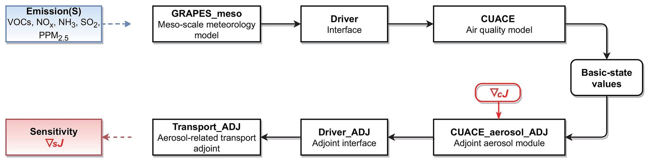
After the TLM and the adjoint model were verified, the GRAPES–CUACE aerosol adjoint model was constructed. The operation flowchart of the adjoint model is shown in Fig. 1. J is the objective function, which can be defined according to the problems concerned. c and s represent state variables (such as BC concentration) and control variables (such as emission sources, mainly including VOCs, NO_x, NH₃, SO₂ and PPM_2.5) in the model, respectively. First of all, the GRAPES–CUACE atmospheric chemistry model should be integrated to store the basic-state values of the unequilibrated variables in checkpoint files. The intermediate values are recalculated or saved in stack using the PUSH&POP method, which pushes the intermediate values into a continuous memory space and pops them out where needed, during the adjoint operating process. Subsequently, the gradient of J with respect to c (∇_cJ) as well as the saved basic-state values are taken as input data for the adjoint backward integration. Finally, the sensitivity of J with respect to s (∇_sJ) can be obtained. A full description of the construction, framework and operational flowchart of the GRAPES–CUACE aerosol adjoint model can be found in An et al. (2016).

Figure 1 Running process of GRAPES–CUACE atmospheric chemistry model and its adjoint model.

2.3 L-BFGS-B method

The limited-memory Broyden–Fletcher–Goldfarb–Shanno algorithm (L-BFGS) is an optimization algorithm in the family of quasi-Newton methods that approximates the BFGS using a limited amount of computer memory (Liu and Nocedal, 1989). The L-BFGS-B algorithm extends L-BFGS to solve large nonlinear optimization problems subject to simple bounds on the variables (Byrd et al., 1995; Zhu et al., 1997), which can be expressed as

$$\begin{array}{}\text{(8a)}& {\displaystyle }& {\displaystyle }minf\left(\mathit{x}\right),\mathit{x}\in R^n,\text{(8b)}& {\displaystyle }& {\displaystyle }\text{subject to}\mathit{l}\le \mathit{x}\le \mathit{u},\end{array}$$

where f is a nonlinear function, the vectors l and u represent lower and upper bounds on the variables, and the number of variables n is assumed to be large. The algorithm is also appropriate and efficient for solving unconstrained problems in which the variables have no bounds. With the supply of the objective function f and its gradient g, but with no requirement of knowledge about the Hessian matrix of the objective function f, the algorithm can be useful for solving large problems where the Hessian matrix is difficult to compute or is dense.

The brief procedure of the L-BFGS-B algorithm is as follows. At each iteration, a limited memory BFGS approximation to the Hessian is updated. The limited memory BFGS matrix is used to define a quadratic model of the objective function f. A search direction d_k is computed by a two-stage approach. First, use the gradient projection method to identify a set of active variables, such as variables that will be held at their bounds. Then, the quadratic model is approximately minimized with respect to the free variables. The search direction is defined to be the vector leading from the current iterate to this approximate minimizer. Finally, a line search is performed along the search direction d_k to compute a step length λ_k, and the variables are updated through ${\mathit{x}}_{k+\mathrm{1}}={\mathit{x}}_k+{\mathit{\lambda }}_k{\mathit{d}}_k$. The L-BFGS-B algorithm has three termination criteria: the number of iterations reaches the set maximum value; the change of the objective function in consecutive iterations is relatively small; and the modulus of the projected gradient is small enough.

3 Description of GRAPES–CUACE-4D-Var

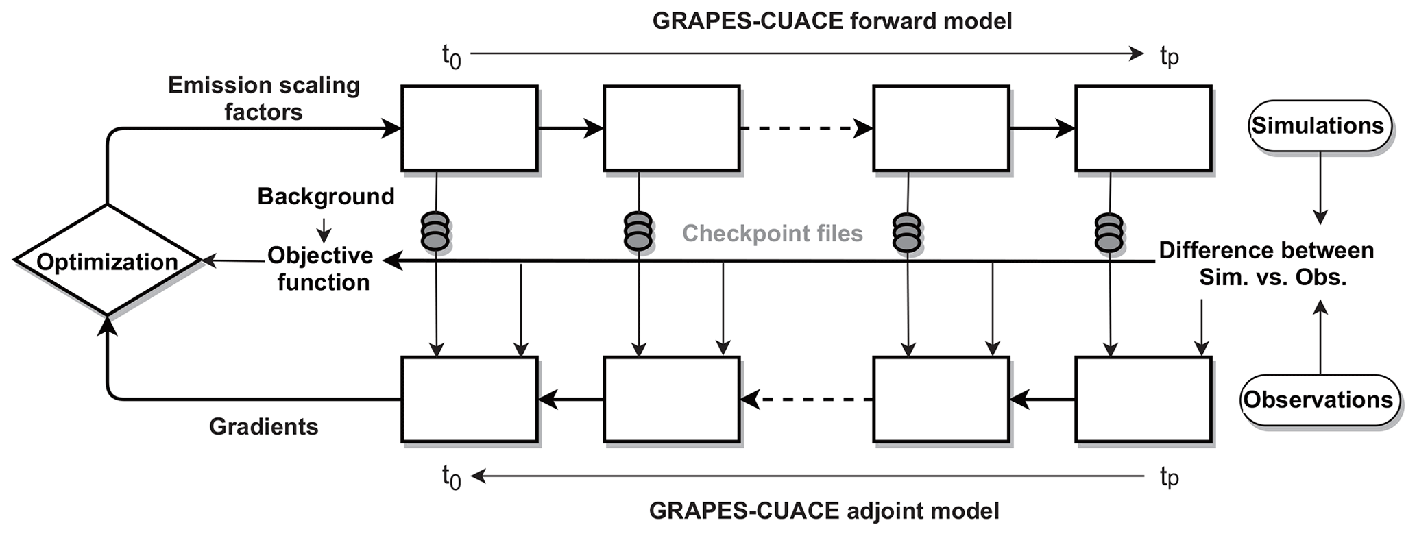
The new 4D-Var data assimilation system, GRAPES–CUACE-4D-Var, was constructed on the basis of the GRAPES–CUACE atmospheric chemistry model, the GRAPES–CUACE aerosol adjoint model and the L-BFGS-B method. A schematic diagram of GRAPES–CUACE-4D-Var is shown in Fig. 2. The main parts of GRAPES–CUACE-4D-Var include GRAPES–CUACE atmospheric chemistry simulation, during which the basic-state values of the unequilibrated variables in checkpoint files are saved, observations and adjoint forcing term processing, GRAPES–CUACE aerosol adjoint model simulation, gradient extraction, cost function calculation, and optimization. The details of cost function, observations and optimization of emission inversion are as follows.

Figure 2 GRAPES–CUACE-4D-Var assimilation system.

3.1 Cost function

Based on Bayesian theory and the assumption of Gaussian error distributions (Rodgers, 2000) the cost function of the emission inversion is generally defined as follows:

$$\begin{array}{}\text{(9)}& \begin{array}{rl}& J\left(\mathit{x}\right)={\displaystyle \frac{\mathrm{1}}{\mathrm{2}}}\mathit{\gamma }{\left(\mathit{x}-{\mathit{x}}_b\right)}^T{\mathbf{B}}^{-\mathrm{1}}\left(\mathit{x}-{\mathit{x}}_b\right)\\ & +{\displaystyle \frac{\mathrm{1}}{\mathrm{2}}}\sum _{i=\mathrm{0}}^p{\left({\mathbf{F}}_i\left(\mathit{x}\right)-{\mathit{y}}_i\right)}^T{\mathbf{R}}^{-\mathrm{1}}\left({\mathbf{F}}_i\left(\mathit{x}\right)-{\mathit{y}}_i\right)\end{array},\end{array}$$

where x, which we sought to optimize, generally represents the state vector of emissions or their scaling factors, x_b is the prior estimate of x, B is the error covariance estimate of x_b, F is the forward model, y is the vector of measurements that are distributed during the time interval [t₀, t_p], R is the observation error covariance matrix, and γ is the regularization parameter.

In this study, we followed the method in Henze et al. (2009), and defined x as the state vector of scaling factors of BC emissions:

$$\begin{array}{}\text{(10)}& \mathit{x}=\ln \left({\displaystyle \frac{\mathit{s}}{{\mathit{s}}_b}}\right),\end{array}$$

where s is the state vector of the daily gridded emissions of BC at three vertical levels (non-point source on the ground, middle-elevation point source at 50 m and high-elevation point source at 120 m) and s_b is the prior estimate of s. Thus, the prior estimate of x(x_b) is equal to 0. According to Cao et al. (2011), the uncertainty of prior BC emissions used in this study is 76.2 %. Therefore, we assigned the prior error covariance matrix (B) to be diagonal and the uncertainty to be 76.2 % for BC emissions. Due to the lack of information to completely construct a physically representative B, the regularization parameter γ is introduced to balance the background and observation terms in the cost function. As described in Henze et al. (2009), an optimal value of γ can be found with the L-curve method (Hansen, 1998). Here, we followed this method and obtained γ=0.0001 through several emission inversions with a range of γ (10, 1, 0.1, 0.01, 0.001, 0.0001, 0.00001, 0.000001, 0.0000001).

3.2 Observations

The surface measurements of BC were collected from the China Atmosphere Watch Network (CAWNET). The CAWNET was established by the China Meteorological Administration to monitor the BC surface mass concentration over China in 2004 and had 54 monitoring stations in the summer of 2016. The monitoring of BC was conducted by an aethalometer (Model AE 31, Magee Scientific Co., USA), which uses a continuous optical greyscale measurement method to produce real-time BC data (Gong et al., 2019). In this study, we used the recommended mass absorption coefficient for the instrument at an 880 nm wavelength with 24 h mean values of BC during 1–31 July 2016 at five representative stations of CAWNET in northern China (Fig. S1 in the Supplement).

The surface PM_2.5 concentrations were obtained from the public website of the China Ministry of Ecology and Environment (MEE) (http://www.mee.gov.cn/, last access: 14 January 2021). The network started to release real-time hourly concentrations of SO₂, NO₂, CO, ozone (O₃), PM_2.5 and PM₁₀ in 74 major Chinese cities in January 2013, which further increased to 338 cities in 2016. The PM_2.5 data were collected by the TEOM1405-F monitor, which draws ambient air through a sample filter at constant flow rate, continuously weighing the filter and calculates the near real-time mass concentration of the collected particulate matter. We used hourly surface PM_2.5 concentrations for 1–31 July 2016 at 48 cities in northern China, including 12 cities in the Beijing–Tianjin–Hebei region (Fig. S1). Here, we have averaged PM_2.5 concentrations at several monitoring sites in each city to represent a regional condition.

To improve the performance of emission inversion, adequate observations are needed for constraining the model. Due to the limited BC monitoring sites in northern China, we used the surface PM_2.5 concentrations at 48 cities described above and the BC∕PM_2.5 ratio to obtain the hourly BC concentrations for 1–31 July 2016 at 48 cities in northern China. The detailed calculation process can be found in the Supplement.

The observation error covariance matrix (R), which is difficult to quantify, generally includes contributions from the measurement error, the representation error and the forward model error (Henze et al., 2009; Zhang et al., 2016; Cao et al., 2018). And there is also a certain error in calculating the BC concentration based on the BC∕PM_2.5 ratio. To reflect the possibly large uncertainties of the observation, we assumed R to be diagonal and with error of 100 %.

3.3 Optimization

Minimization of the cost function Eq. (9) is performed through optimization. Starting from an initial guess (x equal to 0), the forward model simulates BC concentrations at each integration step during the time interval [t₀, t_p], and the adjoint model, which is driven by the discrepancy between simulated and observed BC concentrations, calculates the gradients of the cost function with respect to the scaling factors of BC emission (Fig. 2). Subsequently, the gradients are supplied to the L-BFGS-B optimization routine (Byrd et al., 1995; Zhu et al., 1997) to minimize the cost function iteratively (Fig. 2). At each iteration, the improved estimates of the scaling factors are implemented and the forward and adjoint models are integrated.

3.4 Setup of emission inversion experiment

The simulation domain in this study is northern China (105–125^∘ E, 32.25–43.25^∘ N; Fig. S1), covering 41×23 horizontal grids with a resolution of $\mathrm{0.5}{}^{\circ }\times \mathrm{0.5}{}^{\circ }$ and vertically divided into 31 layers with an integration time step of 300 s. The National Centers for Environmental Prediction Final (FNL) Analysis dataset at a 6 h interval is used as meteorological input. The prior emission used here is the daily gridded BC emission at three vertical levels (non-point source on the ground, middle-elevation point source at 50 m and high-elevation point source at 120 m) mentioned above. The results calculated by the BC∕PM_2.5 ratio show that the BC concentration in Beijing was high on 4 July 2016. So the assimilation window is from 20:00 CST, 3 July, to 19:00 CST, 4 July 2016. The hourly BC concentrations at 36 cities during this time interval are used for the emission inversion, and the BC concentrations of the remaining 12 cities are used for validation of the inversion effect (Fig. S1). The simulation is initialized at 20:00 CST, 30 June; the first 3 d are set as the spin-up time. The convergence criterion used in the optimization is that the objective function decreases by less than 1 % in consecutive iterations. According to the maximum estimation range of the prior emissions, here the upper and lower bounds of the scaling factors of BC emissions are ln(1.6) and ln(0.4), respectively.

4 Results and discussion

4.1 Comparisons between the simulated and observed concentrations

The progression of the cost function at iteration k (J_k∕J₀) during the optimization procedure is shown in Fig. 3. The cost function quickly reduces and reaches the convergence criterion after eight iterations, with values of the converged cost function reduced by 37 %.

Figure 3 Cost function reduction.

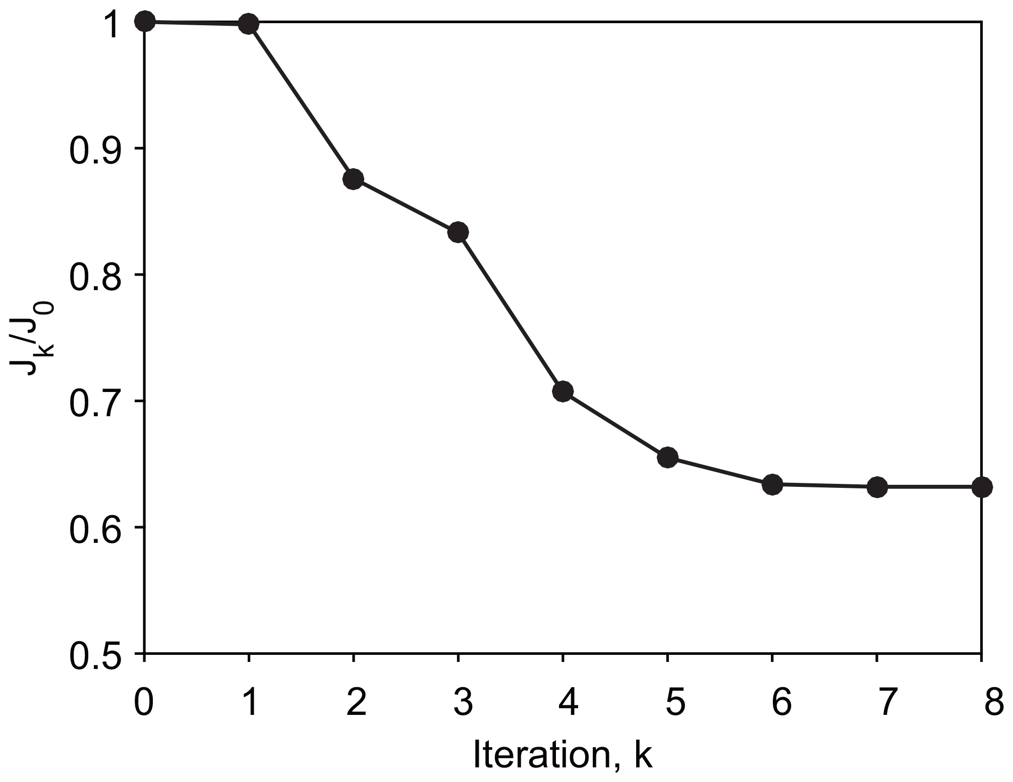
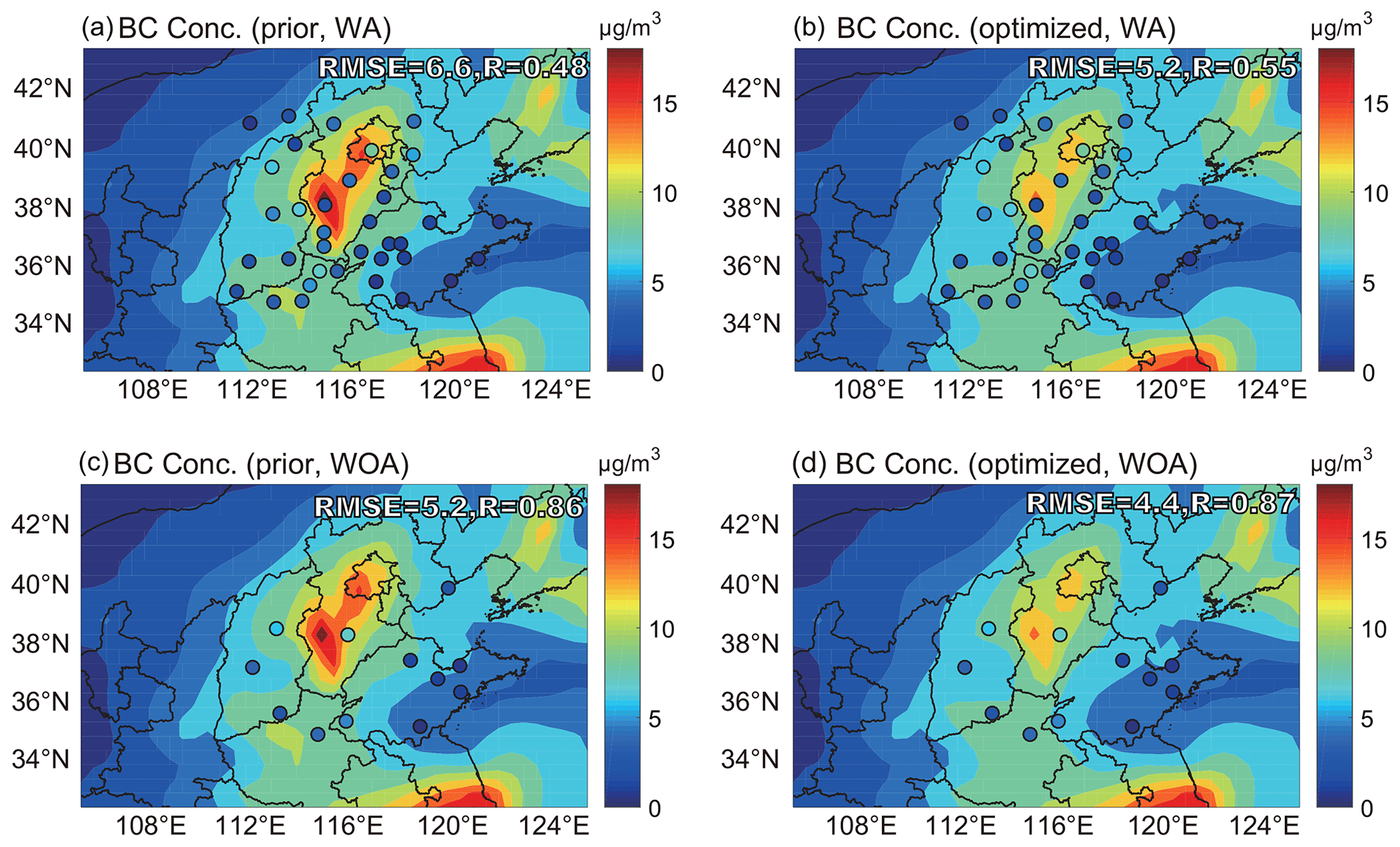
Figure 4 The spatial distribution of observed and simulated daily BC concentrations on 4 July 2016. The observations (circles) are overplotted over model simulations with the (a, c) prior and (b, d) optimized emissions. The observations at 36 cities in (a) and (b) were used in the assimilation, and the observations at 12 cities in (c) and (d) were not used in the assimilation. The root-mean-square error (RMSE) and correlation coefficient (R) between observation and simulation are shown as insets. The observed BC concentrations were calculated by the BC∕PM_2.5 ratio method.

Figure 4 shows the spatial distribution of observed and simulated daily BC concentrations on 4 July 2016. In general, the results simulated with the prior emission reflect the distribution characteristics of BC concentration in northern China to a certain extent, with high values mainly located in Beijing and central and southern Hebei and low values mainly located in Inner Mongolia and eastern Shandong. However, the differences between the simulated and the observed BC concentrations are considerable, and almost all are over-predictions. The optimized (posterior) emissions compensate for the over-predictions and largely reduce the model biases. For instance, the model biases for BC in Beijing, Tianjin, Shijiazhuang, Jinan, Taiyuan and Zhengzhou are reduced by 46 % (from 5.4 to 2.9 µg/m³), 26 % (from 6.6 to 4.9 µg/m³), 29 % (from 18.4 to 13.1 µg/m³), 20 % (from 6.6 to 5.3 µg/m³), 34 % (from 4.1 to 2.7 µg/m³) and 20 % (from 6.9 to 5.5 µg/m³), respectively (Fig. 4a, b). The results simulated with the optimized emission also show improved agreement with the observations over northern China with lower root-mean-square errors and higher correlation coefficients (Fig. 4a, b).

It is crucial to validate the assimilation results by observations that were not utilized in the assimilation. The BC concentrations at 12 cities were used for validation (Fig. 4c, d). Assimilation compensates for over-predictions, reduces the root-mean-square errors (from 5.2 to 4.4) and improves the correlation coefficients (from 8.6 to 8.7). The model biases for BC in Hengshui and Yizhou are reduced by 28 % (from 7.2 to 5.2 µg/m³) and 36 % (from 3.9 to 2.5 µg/m³), respectively. The improvements of the remaining 10 cities are also notable, with values of the model biases reduced by 1 %–20 %.

4.2 Comparisons between the prior and optimized BC emissions

Figure 5 shows the spatial distributions of the prior and optimized daily BC emissions, which are at three vertical levels (non-point source on the ground, middle-elevation point source at 50 m and high-elevation point source at 120 m) as required by the GRAPES–CUACE model. The BC emissions on the ground are mostly non-point sources and at 50 m are concentrated middle-elevation sources; therefore they are distributed in a large area (Fig. 5a, c), while the BC emissions at 120 m are mainly from a few high-elevation point sources, so they are scattered in the area (Fig. 5e). It can be seen that the distributions of optimized BC emissions at three vertical levels are relatively consistent with those of prior emissions (Fig. 5b, d, f). However, the optimized emissions are considerably reduced (Fig. 5b, d, f). Especially for the regions where observation sites are located, such as southern Beijing, Tianjin, central and southern Hebei, northwest Shandong, central Shanxi, and northern Henan, BC emissions decrease significantly. As for the regions where observation sites are not located, such as Liaoning and Jiangsu, BC emissions are almost unchanged. The reason for this phenomenon is discussed in Sect. 4.3.

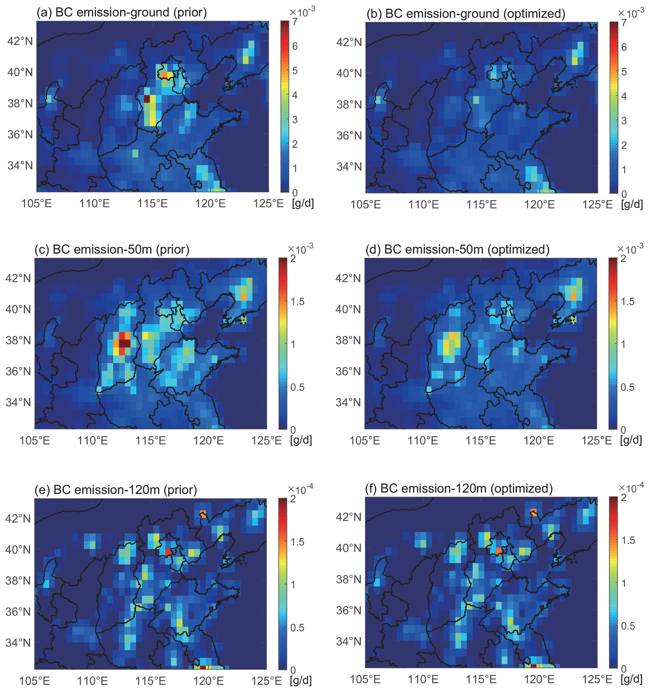
Figure 5 Spatial distributions of the (a, c, e) prior and (b, d, f) optimized daily BC emissions. The emissions are at three vertical levels: (a, b) non-point source on the ground, (c, d) middle-elevation point source at 50 m and (e, f) high-elevation point source at 120 m, as required by the GRAPES–CUACE model.

In order to analyse the differences between the prior and optimized BC emissions in Beijing–Tianjin–Hebei–Shanxi–Shandong–Henan region in more depth and detail, we calculated the ratio of the optimized emissions to prior emissions (optimized emissions divide by prior emissions), as shown in Fig. 6. In general, assimilation has the largest reduction in the non-point source on the ground (Fig. 6a), followed by the middle-elevation point source at 50 m (Fig. 6b), and the smallest reduction in the high-elevation point source at 120 m (Fig. 6c). This is related to the intensity of BC emissions at three vertical levels. The intensity of BC emissions on the ground (Fig. 5a) is about 1–2 orders of magnitude higher than that of the middle-elevation point source at 50 m (Fig. 5c) and the high-elevation point source at 120 m (Fig. 5e). In other words, the BC emissions on the ground have the most significant effect on the overall cost function and therefore reduced most during the progression of assimilation.

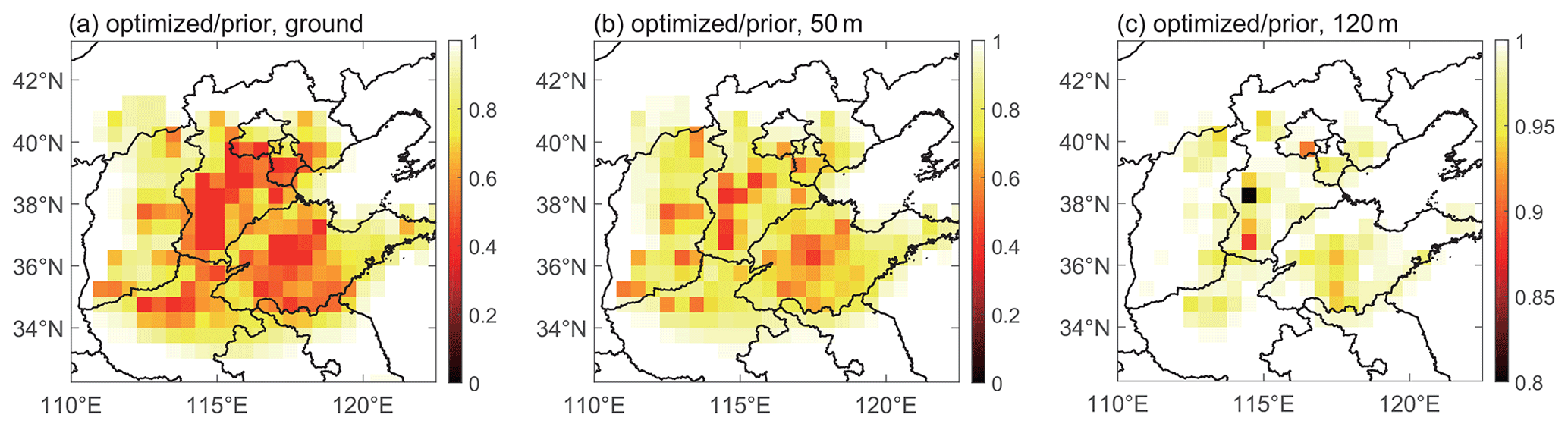
Figure 6 The ratio of optimized emissions to prior emissions (optimized emissions divide by prior emissions). (a) Non-point source on the ground, (b) middle-elevation point source at 50 m and (c) high-elevation point source at 120 m.

The prior BC emissions used in this study are based on statistical data of anthropogenic emissions for 2007 (Cao et al., 2011), and the BC observations used for assimilation are from 2016, so the ratios of the optimized emissions to prior emissions can reflect the changes in BC emissions from 2007 to 2016 to a certain extent. From the perspective of each province, we can see that the ratios of the optimized emissions to prior emissions in Beijing, Tianjin, Hebei, Shanxi, Shandong and Henan are 0.4–0.8, 0.4–0.7, 0.4–0.8, 0.6–0.8, 0.4–0.8 and 0.5–0.8, respectively. This indicates that the BC emissions in these highly industrialized regions have greatly reduced from 2007 to 2016, which is consistent with previous studies (Zheng et al., 2018). Table 1 lists the anthropogenic BC emissions in China by province in 2006 and 2016 and the emission ratios of 2016 relative to 2006. According to previous research, the emission ratios of 2016 relative to 2006 are 0.41–0.82 in Beijing–Tianjin–Hebei–Shanxi–Shandong–Henan region and 0.73 over China. It can be seen that the ratios of the optimized emissions to prior emissions calculated in this study are within a reasonable range, which also shows that the newly constructed GRAPES–CUACE-4D-Var assimilation system can obtain reasonable BC emissions based on the observations.

Table 1 Anthropogenic BC emissions in China by province in 2006^a and 2016^b (units: Gg/year).

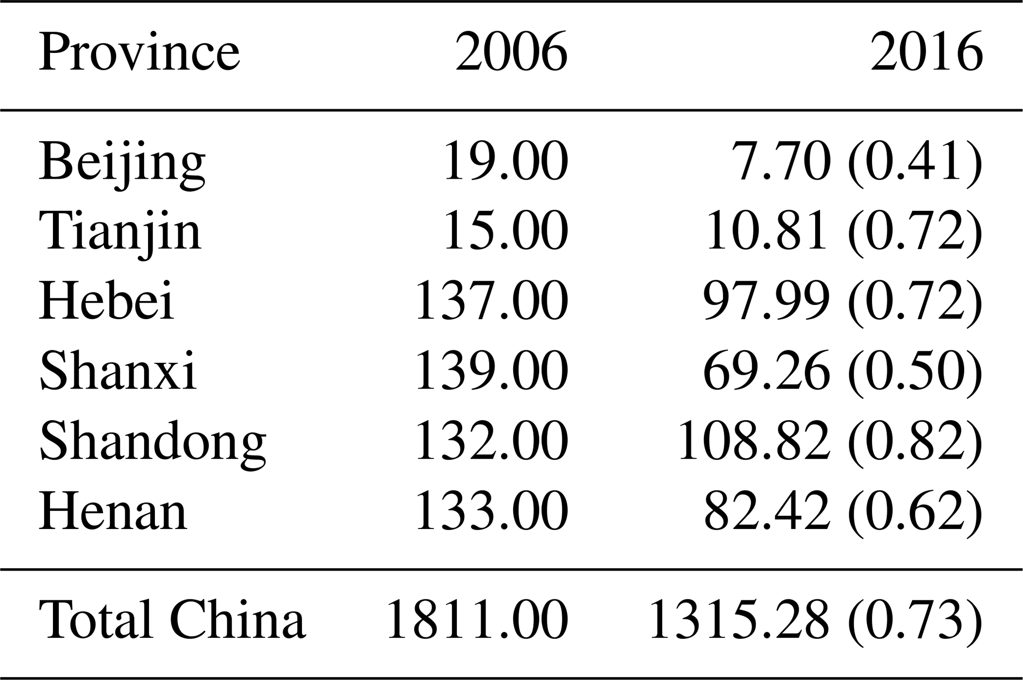
Note: numbers in parentheses represent emission ratios relative to 2006. ^a Source: Zhang et al. (2009). ^b Source: MEIC (Multi-resolution Emission Inventory for China), http://meicmodel.org/ (last access: 14 January 2021).

4.3 Discussion

Although Sect. 4.1 shows that assimilation reduces the model biases and improves all statistical values at each site, there are still over-predictions to a certain degree. In addition to the emission, the initial concentration is also an important factor that affects the BC simulation. Here, we take Beijing as an example to analyse the influence of the initial concentration on the BC simulation. Figure 7 shows the comparison of observed and simulated (with the prior and optimized BC emissions, respectively) BC concentrations in Beijing from 20:00, 3 July, to 19:00, 4 July 2016. At the initial moment (20:00, 3 July 2016), the initial concentration for simulation (11.5 µg/m³) was about 2 times higher than the observations (5.7 µg/m³). With such a high initial concentration, the simulated BC concentrations with prior emissions were significantly higher than the observed concentrations at all times. The simulations with optimized emissions compensated for the over-predictions, but the BC concentrations were still higher than the observations in the first few hours (from 20:00, 3 July, to 02:00, 4 July 2016). And the model bias during this time period was 5.2 µg/m³. As the influence of the initial concentration on the simulation gradually weakened, the simulated BC concentrations with optimized emissions were largely reduced and much closer to the observations from 03:00 to 19:00, 4 July 2016, and the model biases during this time period also decreased, with the value of 1.9 µg/m³. This indicates that for short-term simulation, the influence of initial concentration on the simulation is not negligible. In further work, it is also of great significance to use the GRAPES–CUACE-4D-Var assimilation system to optimize the initial concentration to improve the simulation effect.

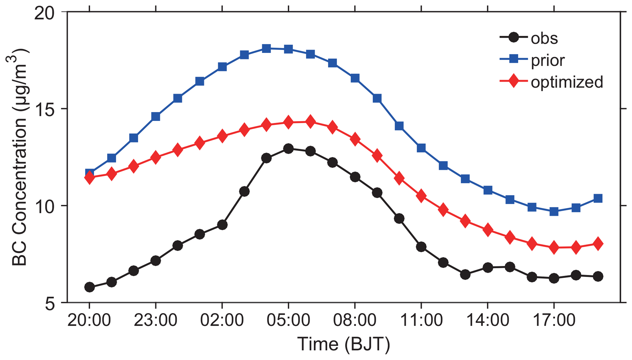
Figure 7 Comparison of observed and simulated (with the prior and optimized BC emissions, respectively) BC concentrations in Beijing from 20:00, 3 July, to 19:00, 4 July 2016. The observed BC concentrations were calculated by the BC∕PM_2.5 ratio method.

As described in Sect. 4.2, after assimilation, the BC emissions in the regions where observation sites are located decrease significantly, while in the regions where observation sites are not located, such as Liaoning and Jiangsu, BC emissions are almost unchanged. This may be due to the short period of the observation data used for assimilation. In this study, since the GRAPES–CUACE-4D-Var assimilation system has not yet implemented parallel computing, the assimilation window was set for 24 h. In such a short period of time, the pollutants emitted from Liaoning and Jiangsu may not have been transported to the regions where observation sites are located, thus having little impact on the BC concentrations in these regions. In other words, the emissions from Liaoning and Jiangsu have little effect on the overall cost function, so there is little change during the progression of assimilation. Therefore, implementing parallel computing of the GRAPES–CUACE-4D-Var assimilation system and performing emission inversion for a longer period (i.e. 1 month) is another important task in the future.

5 Conclusions

In this study, we developed a new 4D-Var data assimilation system for the GRAPES–CUACE atmospheric chemistry model (GRAPES–CUACE-4D-Var) and applied it for assimilating surface BC concentrations and optimizing its daily emissions in northern China on 4 July 2016, when a pollution event occurred in Beijing. The main conclusions are as follows.

• The newly constructed GRAPES–CUACE-4D-Var assimilation system is feasible and can be applied to perform BC emission inversion in northern China.

• The BC concentrations simulated with optimized emissions show improved agreement with the observations over northern China with lower root-mean-square errors and higher correlation coefficients. The model biases are reduced by 20 %–46 %. The validation of assimilation results with observations that were not utilized in the assimilation shows that assimilation compensates for over-predictions, reduces the root-mean-square errors and improves the correlation coefficients. The improvements are also notable, with values of the model biases reduced by 1 %–36 %.

• Compared with the prior BC emissions, the optimized emissions are considerably reduced. Especially for Beijing, Tianjin, Hebei, Shandong, Shanxi and Henan, the ratios of the optimized emissions to prior emissions are 0.4–0.8, indicating that the BC emissions in these highly industrialized regions have greatly reduced from 2007 to 2016, which is consistent with previous studies.

In the following work, implementing parallel computing of the GRAPES–CUACE-4D-Var assimilation system and performing emission inversion for a longer period is an important task. Apart from the emissions, the initial concentration is also an important factor for short-term simulation. It is of great significance to use the GRAPES–CUACE-4D-Var assimilation system to optimize the initial concentration to improve the simulation effect.

Meanwhile, several mega urban agglomerations in China are facing atmospheric compound pollution with high PM_2.5 and O₃ concentrations (Li et al., 2019; Zhang et al., 2019; Xiang et al., 2020; Haque et al., 2020; Zhao et al., 2020). To improve air quality, it is urgent to formulate reasonable and effective emission-reduction measures. Therefore, further studies on expanding the function of the GRAPES–CUACE-4D-Var assimilation system and taking into account factors such as air quality standards, the proportion of emissions that can be reduced, the economic cost and residents' health benefits of emission reduction are crucial for formulating optimized pollution-control strategies for PM_2.5 and O₃ in China.