the Creative Commons Attribution 4.0 License.
the Creative Commons Attribution 4.0 License.
 | 31 May 2021
Radiative Transfer Model 3.0 integrated into the PALM model system 6.0
Jaroslav Resler
Matthias Sühring
Sebastian Schubert
Mohamed H. Salim
Vladimír Fuka
The Radiative Transfer Model (RTM) is an explicitly resolved three-dimensional multi-reflection radiation model integrated into the PALM modelling system. It is responsible for modelling complex radiative interactions within the urban canopy. It represents a key component in modelling energy transfer inside the urban layer and consequently PALM's ability to provide explicit simulations of the urban canopy at metre-scale resolution. This paper presents RTM version 3.0, which is integrated into the PALM modelling system version 6.0. This version of RTM has been substantially improved over previous versions. A more realistic representation is enabled by the newly simulated processes, e.g. the interaction of longwave radiation with the plant canopy, evapotranspiration and latent heat flux, calculation of mean radiant temperature, and bidirectional interaction with the radiation forcing model. The new version also features novel discretization schemes and algorithms, namely the angular discretization and the azimuthal ray tracing, which offer significantly improved scalability and computational efficiency, enabling larger parallel simulations. It has been successfully tested on a realistic urban scenario with a horizontal size of over 6 million grid points using 8192 parallel processes.
- Article
(4027 KB) - Full-text XML
-
Supplement
(525 KB) - BibTeX
- EndNote


1.1 Overview of current solutions
Accurate representation of spatio-temporal radiative exchange processes is essential for realistic modelling of the atmospheric boundary layer, especially with the urban boundary layer. These processes determine the energy budget of the surfaces and thus strongly affect boundary-layer dynamics as well as the spatio-temporal distribution of temperature, moisture and other scalar variables. In contrast to synoptic-scale and mesoscale atmospheric models, microscale and building-resolving models encounter considerable challenges to accurately model such processes due to their fine spatial resolution and the heterogeneity of urban environments.
Many urbanized mesoscale models consider the vertical and horizontal radiative exchange within the urban canopy layer, including shading and multiple reflections, by assuming a strongly simplified urban surface structure (Grimmond et al., 2010). Urban surfaces are typically oriented in a quasi-two-dimensional street canyon (e.g. Masson, 2000; Kusaka et al., 2001; Martilli et al., 2002; Lee and Park, 2008; Schubert et al., 2012; Mussetti et al., 2020) or regularly spaced single buildings of equal size (e.g. Kondo et al., 2005). On the building-resolving microscale, such simplifications are not possible, and the complex shapes of obstacles (e.g. buildings, terrain or vegetation) need to be resolved. This, however, increases the complexity of the numerical solution and creates difficulties with respect to parallelization strategies via horizontal domain decomposition, which is commonly applied in atmospheric models (Tang et al., 2020), as the direct horizontal exchange is no longer limited to neighbouring subdomains.
Consequently, the method and the sophistication of modelling the radiative exchange within the urban boundary layer vary in microscale atmospheric models (Krayenhoff and Voogt, 2007; Huttner and Bruse, 2009; Heus et al., 2010; Früh et al., 2011; Gross, 2012; Franke et al., 2012; Yang and Li, 2013; Krayenhoff et al., 2014; Salim et al., 2018; more recently1 Kim et al., 2020, and Lee and Lee, 2020). They range from applying a simple parameterization of radiative transfer, or even neglecting these processes altogether, to more explicit methods of radiative modelling.
However, some of the microscale models with more explicit radiative modelling have limitations in simulating realistic urban domains. For example, some models use only the Reynolds-averaged Navier–Stokes (RANS) method for simulating the airflow, which is not always suitable for the geometrically complex and highly heterogeneous urban environments. Also, some of the mentioned models are not suitably designed and parallelized to work on high-performance supercomputers (HPCs) with hundreds or thousands of CPU cores, which makes the design and implementation of the explicit 3-D radiative exchange easier, but it severely limits the size and resolution of the modelled domains.
The RTM version 1.0 (Resler et al., 2017) was created in order to provide an open-source, HPC-enabled, fully 3-D model of radiative interactions inside the urban canopy integrated into an urban climate model based on the large-eddy simulation (LES) method. Version 3.0 described in this paper provides substantial improvement over version 1.0 by including a wider selection of simulated processes for better representativity. It also features a new method of discretization and improved algorithms as well as technical implementation for enhanced scalability and computational efficiency.
1.2 RTM role within the PALM model
Radiation processes are traditionally modelled in PALM by a one-dimensional radiation model with simulation of vertical radiation exchange without any lateral interactions (Maronga et al., 2015). The particular type of radiation model can be selected and configured based on the requirements of the modelled scenario. The Rapid Radiative Transfer Model for Global models (RRTMG; see Clough et al., 2005) is available in addition to a simpler clear-sky model (Maronga et al., 2020). Alternatively, users can prescribe a constant net radiation at the surfaces or use an external radiation input, such as observation data or a meteorological model output, for a better representation of cloud cover.
This one-column approach, however, is not sufficient to model the surface energy balance inside the urban canopy layer. This area is typically characterized by complex geometry of terrain, buildings and vegetation, for which the radiative transfer processes in all directions cannot be neglected. Therefore, the PALM modelling system includes the Radiative Transfer Model (RTM) as part of PALM-4U (PALM components for urban modelling). This model takes the radiation from the PALM radiation model, e.g. RRTMG, as input and calculates the radiation processes taking place inside the urban canopy layer explicitly in a fully 3-D geometry. Through this, RTM provides the radiative fluxes and the surface net radiation including its components on the 3-D geometry, which are then used to model the surface energy balance, evapotranspiration in the plant canopy, and biometeorological quantities (see Sect. 4).
The main goals of the RTM development were to create a computationally efficient model which simulates all substantial radiative processes taking place inside the urban canopy and which is fully integrated with the rest of the PALM model and its components, in particular
-
the spatial discretization of the domain matches the discretization of other parts of the PALM model;
-
RTM is executed as part of the PALM programme, and it utilizes its parallelization scheme; and
-
RTM utilizes PALM data structures and subroutines as much as possible and provides its results directly back to PALM and its modules.
1.3 Changes since RTM version 1.0
The paper describes version 3.0 of RTM, which is part of PALM version 6.0. This paper is a follow-up paper to Resler et al. (2017), which describes RTM version 1.0 as part of the Urban Surface Model version 1.0 (PALM-USM) integrated into PALM version 4.0.
RTM version 1.0, as part of the PALM-USM module, has been evaluated with respect to performance and accuracy on a small urban scenario in Prague–Holešovice (Resler et al., 2017). The most important changes between RTM 1.0 and RTM 3.0 include the following.
-
New discretization schemes for direct solar irradiance and for the sky view, which includes diffuse solar irradiance, longwave irradiance from the sky and reflection as well as emissions from surfaces towards the sky (see Sect. 2.3).
-
A new discretization scheme for the reflected and emitted radiation between surfaces (Sect. 2.2.4).
-
The novel azimuthal ray-tracing algorithm (Sect. 3.1).
-
Plant canopy interaction with LW radiation (absorption and emission, Sect. 2.4.2).
-
Evapotranspiration and latent heat flux in the plant canopy (Sect. 4.3).
-
Bidirectional integration with the radiation forcing model (e.g. RRTMG, Sect. 4.1).
-
Calculation of mean radiant temperature for selected levels aboveground with provision of radiant fluxes for the biometeorology module (Sect. 2.5).
-
Integration of RTM within the PALM radiation module and coupling to all surface modules (Sect. 4.2).
-
Multiple improvements, bug fixes and changes in interfaces with other PALM modules.
In order to quantify the differences brought by the new simulated processes and improved discretization schemes, a comparison study has been performed on the same scenario using PALM version 6.0 with RTM 3.0 with different sets of newly available simulated processes enabled. The results of this comparison are available in Krč (2019).
The paper is organized as follows: Section 2 describes the numerical approaches used in the RTM to consider the relevant physical radiation processes, while Sect. 3 describes the implementation of the RTM in PALM. Section 4 gives an overview of how the RTM interconnects with other PALM modules. An evaluation of the RTM and a discussion of computational performance issues are presented in Sect. 5. Finally, Section 6 closes with a summary and ideas for further developments.
The PALM model discretizes the modelled domain using a regular three-dimensional grid. The model supports arbitrary rotation of the grid around the vertical axis, with the default having the x dimension representing the east–west axis in the eastward direction and the y dimension representing the south–north axis in the northward direction. The z dimension always represents the vertical axis in the upward direction. Considering that the modelled domains are relatively small within the order of kilometres, PALM uses an f-plane approximation (constant Coriolis parameters within the model domain) with equidistant horizontal grid spacing rather than any spherical or ellipsoid geodetic projection.
The x and y dimensions of the PALM grid are equidistant, so the grid is always regular, although the resolution of the x and y dimensions may differ. The vertical axis may employ progressive stretching, which should only be applied well above the boundary layer; otherwise, a bias could be introduced to the vertical turbulent transport. Also, the RTM requires an equidistant grid inside the urban layer in which it operates.
For each horizontal coordinate (x,y), PALM specifies a terrain height, which is discretized according to the vertical grid spacing, meaning that each grid box is either completely above or below the surface. When representing urban areas, the obstacles include any permanent solid objects, e.g. buildings or terrain unevenness, while trees, shrubs and other resolved plant volumes are modelled separately as the plant canopy. Terrain and buildings in RTM are currently limited to a so-called 2.5-D geometry, which is able to represent radiative processes at upward-facing and horizontally facing surfaces and thus covers the majority of natural and large urban objects. Although PALM is also able to represent downward-oriented surfaces, e.g. bridges or overhanging parts of buildings for which its effect on the flow field is considered, RTM version 3.0 does not consider them in radiative interactions yet.2 The model grid divides the 2.5-D surface geometry into individual surface grid elements, which are referred to as faces. The 2.5-D geometry is plane-parallel, so a face can be oriented northward, southward, westward, eastward or upward.
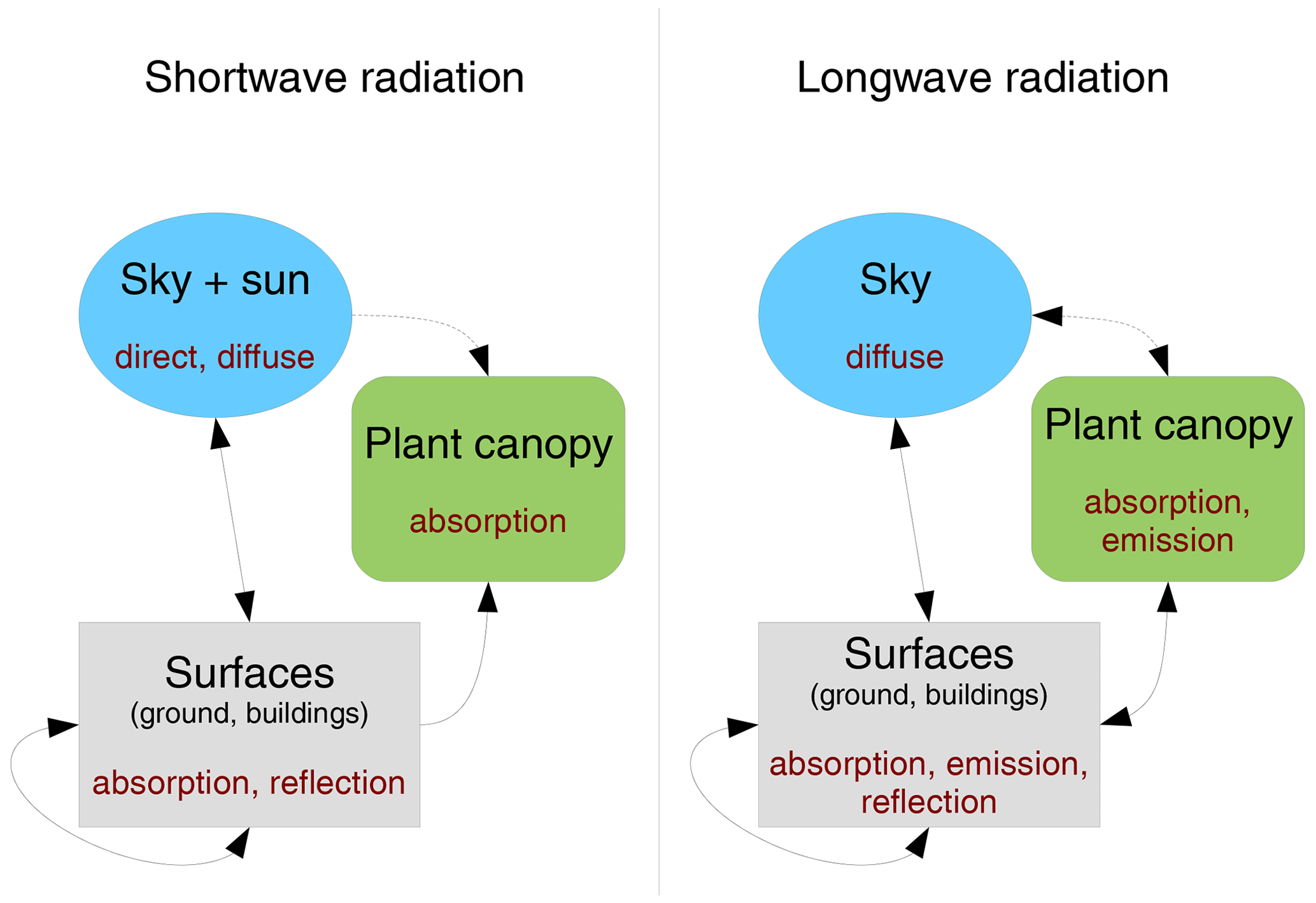
The RTM considers two spectral ranges of electromagnetic radiation independently: shortwave (SW) visible solar radiation and longwave (LW) thermal radiation. The modelled radiation originates from the sun, the atmosphere and all the modelled surfaces. The result of RTM is the amount of absorbed, reflected and emitted radiation for every face (both horizontal and vertical) and the amount of absorbed and emitted radiation for each grid box containing resolved plant canopy (plant canopy grid box, PCGB). The model follows the radiation as it spreads from sources and as it propagates through the urban canopy layer and reflects off individual faces, taking into account model geometry, shading and mutual visibility between the faces, partial transparency and/or opacity of the plant canopy, and reflective properties of the individual faces. Figure 1 gives an overview of the simulated processes. The detailed study of the contribution of the particular processes to the total simulated radiative fluxes is described in Salim et al. (2020).
To limit the computational effort to a reasonable level, some less important processes have to be simplified or disregarded. These are the following.
-
Finite number of reflections. The model simulates a configured number of reflections, after which the residual radiation is considered to be fully absorbed by the respective face it hits. This amount of radiation absorbed after the last reflection is also available among the model outputs, allowing the model to be configured with an appropriate number of reflections so that the remaining amount is negligible. Depending on surface properties and model geometry, between three and five reflections are usually suitable for real-world urban scenarios (see Sect. 5.3). While Yang and Li (2013) consider an infinite number of reflections in their scheme by calculating the Gebhart factor (Gebhart, 1971), they propose limiting this number to greatly reduce the computational demand.
-
Diffuse reflection only. The current version of the model only supports diffuse (non-directional) reflection; specifically, all surfaces are considered Lambertian reflectors. Modelling specular reflection is planned for later versions of the model to better simulate glass and polished surfaces, which are also present among typical urban surfaces. However, in order to simulate correct angles of reflection from surfaces that are not grid-aligned, this feature depends on the addition of arbitrarily oriented faces to PALM. Arbitrarily oriented faces are planned for the next major revision of PALM (see Sect. 6, Outlook).
-
Fully transparent air. Neither absorption, scattering, nor thermal emission by air mass is modelled inside RTM, considering rather short ray paths in the urban canopy layer. In particular for fog, dense smog or heavy precipitation events, this may become relevant, making RTM less suitable for simulating such scenarios. However, RTM only concerns the urban layer. If RRTMG is configured as the radiation model in PALM, it simulates the air mass interaction for the full height of the PALM domain within a one-dimensional framework.
-
Selected processes of plant canopy interaction. Modelling of plant canopy within RTM focuses mainly on its effects on other surfaces and on overall energy balance. In order to reduce computational complexity, it simplifies or disregards some processes which are more relevant to fluxes within the plant canopy itself: reflection from the plant canopy and internal interactions (emission and absorption among adjacent PCGBs). The reasons and impacts are discussed in Sect. 2.4 and internal interactions specifically in Sect. 2.4.2.
-
Zero thermal capacity of plant leaves. Typical plant leaves are thin and lightweight, having a very small thermal capacity with respect to their surface area. This leads to rapid equalization of their temperature with the temperature of the surrounding air via sensible and latent heat flux. In RTM, the simulated thermal capacity of plant leaves is zero and their temperature is identical to that of the surrounding air. This means that the plant canopy heat flux (net radiative flux and also latent heat flux provided by the plant transpiration model; see Sect. 4.3) is directly applied to the air mass. This approach is common in the field of atmospheric modelling (see e.g. Dai et al., 2003). Furthermore, Swenson et al. (2019) showed that for nonforested locations with low biomass amounts their parameterization of biomass heat storage provides similar results as simulations that lack a representation of vegetation heat storage.
2.1 Representing radiative interactions using view factors
The discretization of RTM uses the same Cartesian grid as the rest of the PALM model. Each radiative quantity is modelled as a singular value per surface discretization unit (face), and the propagation of radiation is described as interactions between mutually visible faces.
The model considers all reflections and emissions to be Lambertian (i.e. ideally diffuse), following Lambert's cosine law whereby the amount of radiation leaving the surface in one direction is proportional to the cosine of the angle θ between that direction and the surface normal. The interaction between faces can therefore be described similarly for reflection and for thermal emission.
For any two mutually visible faces i and j, the view factor (VF) Fi→j is the fraction between the radiant flux originating from face i that strikes face j and the total radiant flux leaving face i (e.g. Hamilton and Morgan, 1952; Sparrow and Cess, 1978). In an enclosed system in which all radiative transfer happens between faces , the energy is conserved and the sum of all view factors from each particular face i equals 1:
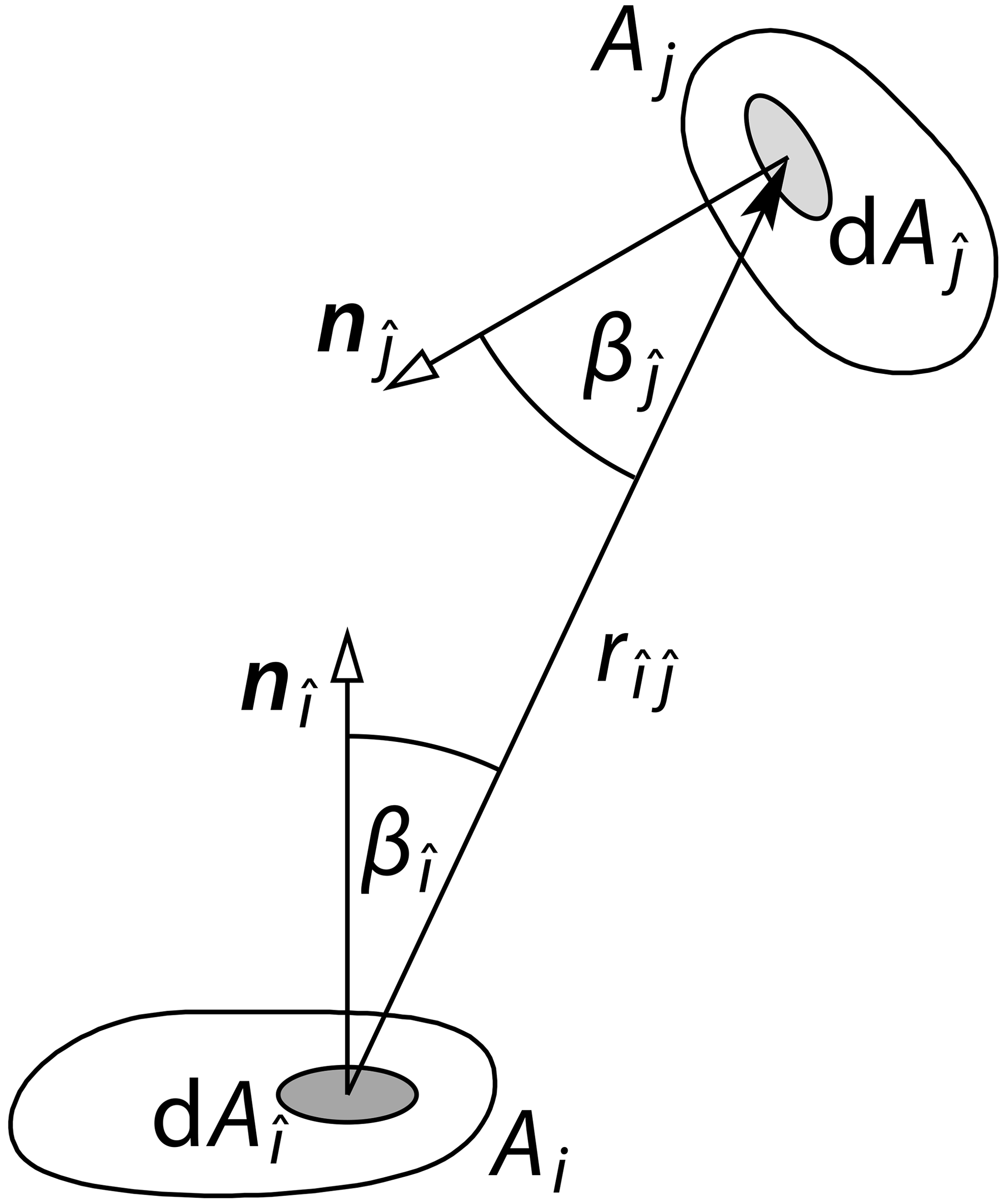
Figure 2Calculation of the view factor between surface Ai and Aj by integrating over Ai and Aj. and are the respective normal vectors of the surface elements and , which are apart.
The value of Fi→j is calculated by integrating over the areas Ai and Aj (see Fig. 2):
Here, is the distance between the surface elements and . and are the angles between the normal vectors of the respective surface element and their connection. Note that the integral is symmetrical for faces i and j, which leads to the reciprocity property . Applying that to Eq. (1), we get for each target face i
This formula allows for the description of the face i, now being considered the target for incoming radiation, as an observer whose field of view is a sum of portions. Each portion represents the view in the direction of a specific source face j, while the size of that portion takes into account the respective solid angle and the cosine law. The fraction is further called the irradiance factor j→i because it can be used to calculate the total irradiance Ei of face i using known radiosities of other faces and the irradiance factor values, which are equal to view factor values in the opposite direction:
where is the total radiant flux received by the target face i, is the radiant flux leaving the source face m and Jm is the radiosity of the face m. It can be seen that the irradiance of face i is the weighted average of radiosities of other faces for which the weights are equal to the irradiance factors.
Precalculated view factor values
The view factor values carry all the information about the geometry of the urban layer necessary for calculating propagation of reflected and emitted light among surfaces. Once they are known, calculation of the instantaneous fluxes can be reduced to simple vector multiplication. Determining the view factor values consists of multiple steps.
-
Establishing mutual orientation and position. In the rectangular grid, this is a matter of performing multiple coordinate comparisons to find out whether, for each face, the other face lies in the half-space above the plane of the first face, i.e. whether its angle θ is less than .
-
Determining obstacles on the ray path between the faces. The obstacles may be fully opaque (terrain, buildings) or partially transparent, in which case a fraction of the radiant flux between the faces is absorbed. In RTM, the only partially transparent obstacle is the grid-resolved plant canopy, which is represented as a 3-D field of leaf area density (LAD). The fraction of the radiant flux allowed to pass through the obstacle and the radiant flux carried by the ray upon striking the obstacle is called transmittance. For the plant canopy, it depends on the length of the ray's intersection with the respective PCGB, the LAD value at that PCGB and the extinction coefficient.
-
Calculating the actual view factor value. Although the exact value for two rectangular faces could be solved as a quadruple integral for each point of each of the faces as in Eq. (2), RTM uses simplifications in order to avoid the exact calculation. Details and reasoning are presented below in Sect. 2.2.
The second step is implemented in RTM using a ray-tracing algorithm. This process is computationally complex, as it performs calculations involving each grid box that each traced ray intersects, and it can also cause very high demands on the interprocess communication (see Sect. 2.2.2 and 2.2.6). In PALM, each parallel process is responsible for modelling a horizontally divided subdomain within the modelled domain, and most of the data stored locally are limited to the extent of the subdomain. Depending on the provided interconnecting infrastructure and the Message-Passing Interface (MPI) implementation, access to the values in other subdomains carried by MPI interprocess communication may be significantly slower than similar local memory access. Depending on the domain size and geometry, each traced ray may cross many subdomains. The complexity of this processing is further examined in Sect. 2.2.2 and 2.2.6.
Due to this complexity, the ray-tracing task takes place during the model initialization phase before the actual simulation of time steps begins. The values representing the view factors and other relevant data are precomputed, exchanged among the parallel processes and stored in such a way that the number of calculations and MPI communications performed during computation of time steps is minimized.
2.2 Discretization of the view in RTM
RTM version 3.0 offers two selectable methods for simulation of the irradiance of each face by providing two different schemes for discretization of the view from each face, which is represented by a set of irradiance factors. The legacy discretization scheme (originally introduced in RTM version 1.0; see Resler et al., 2017) simulates the view from each target face as a set of irradiance factors from the centre of each face that is visible from the target face's centre. This leads to the requirement of performing ray tracing between each pair of mutually visible faces and to the worst-case complexity of 𝒪(n4) with respect to domain size, as is described later in Sect. 2.2.2. Simulating radiative interactions using a set of view factors among discretized surfaces is an established technique. More specifically, using surfaces discretized by a regular grid can be found in e.g. Krayenhoff and Voogt (2007).
The current angular discretization scheme uses a different simplification with a better trade-off between complexity and accuracy and a guaranteed worst-case total number of view factors of 𝒪(n2) (see Sect. 2.2.6). It also uses a newly developed 2-D ray-tracing algorithm which is optimized with respect to CPU time, memory consumption and MPI interprocess communication by utilizing the geometric properties of the discretization scheme. This is a novel technique, and we have not found any reference to using angular discretization for view factors among surfaces. Also, the technique of 2-D ray tracing, which performs ray tracing for whole vertical columns by taking advantage of the specific data representation and parallelization scheme of the model, is novel.
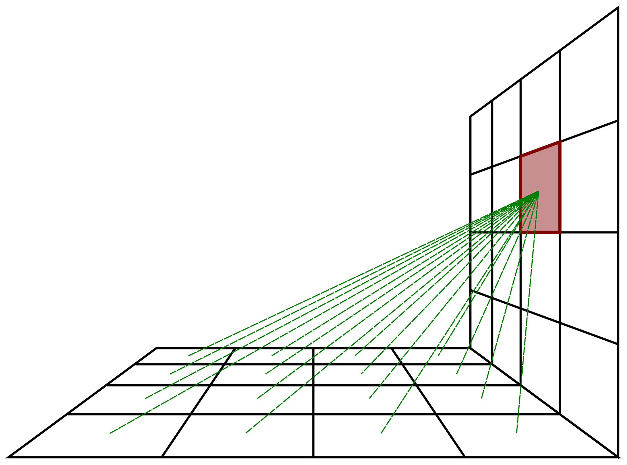
Figure 3Illustration of the legacy view discretization scheme. For the highlighted face, ray tracing is performed between its centre and the centres of its visible faces, creating a set of its view factors.
2.2.1 Legacy discretization of the view
While establishing the mutual visibility between two faces, the path between the faces is represented by a single ray connecting their centres. This is in accordance with the general principle of discretization by a rectangular grid, on which the area or volume covered by each face or grid box is represented by a single scalar value and the resolution can be increased for more spatial precision at the expense of computational resources (see Sect. 2.2.2 and a related case study in Sect. 5.1). This way only one ray needs to be traced for every two faces oriented towards each other, and mutual visibility (absence of shading by an intermediate solid obstacle, i.e. building or terrain) becomes a binary relation. In reality, however, any face may be illuminated only on part of its area, and each target point illuminated by a non-point light source may lie in the penumbra of an obstacle. For the purpose of calculating the radiant flux absorbed by semi-opaque objects, it is assumed that the single ray between face centres carries the whole radiant flux leaving the source face towards the target face.
Together with simplifying the ray tracing, the view factor value calculation is also simplified. Instead of solving the full integral in Eq. (2), the value of the integrand at the centres Ci and Cj of faces i and j, respectively, is used to estimate the full integral. With this, the approximate view factor is given by
The induced error is smaller for very distant faces and larger for faces close to each other. This error is considered acceptable within the resolution of the model, as it can always be reduced by increasing the resolution. The more important issue of this approach is that the sum of the approximate view factor values is no longer guaranteed to equal 1. Because of this, the modelled system could artificially gain or lose energy and possibly even diverge exponentially in time. To guarantee the conservation of energy, the normalization of the approximate view factor values is used in order to maintain Eq. (3), and the normalized view factor is thus calculated by
2.2.2 Computational complexity of the legacy discretization
The asymptotic complexity and scalability of the RTM can be evaluated using two different approaches: considering either a domain growing in size horizontally, while the vertical size and typical shapes of obstacles are kept constant, or considering a gradually increasing resolution for the same domain, which increases the amount of discretized data in each dimension.
The complexity and scalability for the latter case can be determined exactly. The number of faces increases proportionally with the surface area. For a domain with a size of grid cells for which the resolution is increased by a factor φ to grid cells, the number of faces grows exactly by φ2 (because surfaces are two-dimensional) and the number of other faces, to which each face has direct visibility, also grows by φ2. Therefore, the number of view factors grows by φ4. The separation distance in terms of the number of grid boxes between each pair of mutually visible faces, which determines the time needed to perform the ray tracing for such a ray, grows by φ; therefore, the total ray-tracing time grows by φ5.
In order to analyse the scalability of the algorithm, assume that the number of processes used for the calculation grows by the same factor as the size of the 3-D grid, i.e. by φ3. In this situation, the computational demands of each process grow by φ2, and the proportion of interprocess MPI data exchange relative to the process local memory access also increases in both the ray-tracing and the time-stepping part of RTM, so the process does not scale well.
The situation is better in the first case in which the domain of size n×n grid points grows horizontally, and the average terrain height does not change. For typical terrain and building profiles, the average distance of the visible horizon does not increase with the horizontal scaling, or it increases much less than linearly. That also means that the average number of other faces, to which each face has direct visibility, does not increase significantly. This property also helps to keep the computation more localized for parallelism. However, these assumptions are valid for a typical scenario only, while the worst-case complexity is still of the order of 𝒪(n) for ray-tracing distance and 𝒪(n5) for the total computational demands of ray tracing.
2.2.3 Reducing the number of view factors in the legacy discretization
To reduce the high number of view factors with the legacy discretization scheme, RTM allows for the exclusion of some view factors that are considered less important. First, a minimum value Fmin of the irradiance factor can be specified. When faces i and j are mutually visible but the source face i occupies so small a portion of the view from the target face j that the value of the irradiance factor is less than Fmin, then this irradiance factor is disregarded. Thanks to the fact that the potential value of the irradiance factor can be established even before the ray tracing from face i to face j begins, the ray tracing is skipped altogether for such face pairs. In addition to the minimum irradiance factor value, a maximum ray-tracing distance smax can also be specified. This limit avoids starting the computationally intensive ray-tracing routine for such face pairs for which the mutual distance is above the limit.
The normalization described in Sect. 2.2.1 ensures that the remaining irradiance factors are increased accordingly in order to maintain energy conservation by the condition
where is the normalized irradiance factor from face m and is the sky-view factor representing the view towards the sky (described later in Sect. 2.3). Both Fmin and smax have to be chosen carefully considering the geometry of the modelled domain so that the impact on radiative energy balance in the model is not too high.
2.2.4 Angular discretization of the view
The asymptotic complexity of the legacy scheme does not allow simulations of very large domains with horizontal sizes of the order of millions of grid boxes or more. Furthermore, if the view from some face is composed of both very close and very distant faces, the computational resources are used unevenly: proportionally fewer resources are spent on close faces, each of which represents a higher share of the face's view and also a potentially greater share of its irradiance, while more resources, often a majority, are spent on less relevant distant faces. Neglecting the smaller view factors as described in Sect. 2.2.3 and normalizing the result also represent a possible way to combat this disproportion. This approach, however, has to be used carefully because it can significantly alter the ratio between a face's irradiance from close and distant surfaces, which could introduce a systematic bias in radiant fluxes coming from the close and distant surfaces.
Thus, we introduce a novel angular discretization scheme for reflected and emitted radiation. The general motivation for this approach is based on the observation that the properties of most surfaces are smooth in space, and thus two faces next to each other tend to have similar properties and radiate similarly more often than two generic unrelated faces. This consideration leads to the idea of representing a target face's irradiation from multiple neighbouring distant faces by a single view factor that uses the radiation from one of them, but its view factor value represents all of them. This approach allows for the use of the computational resources more efficiently.
The angular discretization scheme divides the view from each face into a fixed number of directions specified by uniformly distributed azimuth and elevation angles, as opposed to the uneven set of directions towards the centres of every other visible face in the legacy discretization scheme. Ray tracing is performed towards this fixed set of directions with considerable optimization due to the fact that multiple rays of this set share an identical horizontal direction (i.e. azimuth; see Sect. 3.1). For each ray, the face that covers the first detected obstacle (terrain or building) is used to create a view factor entry. Its view factor value represents exactly the portion of the view corresponding to its direction segment (the section of azimuths and elevations instead of being determined by the other face's size and position). Figure 4 depicts the geometry of the discretization and also demonstrates the Nusselt analogue, which can be used to visualize the relative sizes of the view factor values.
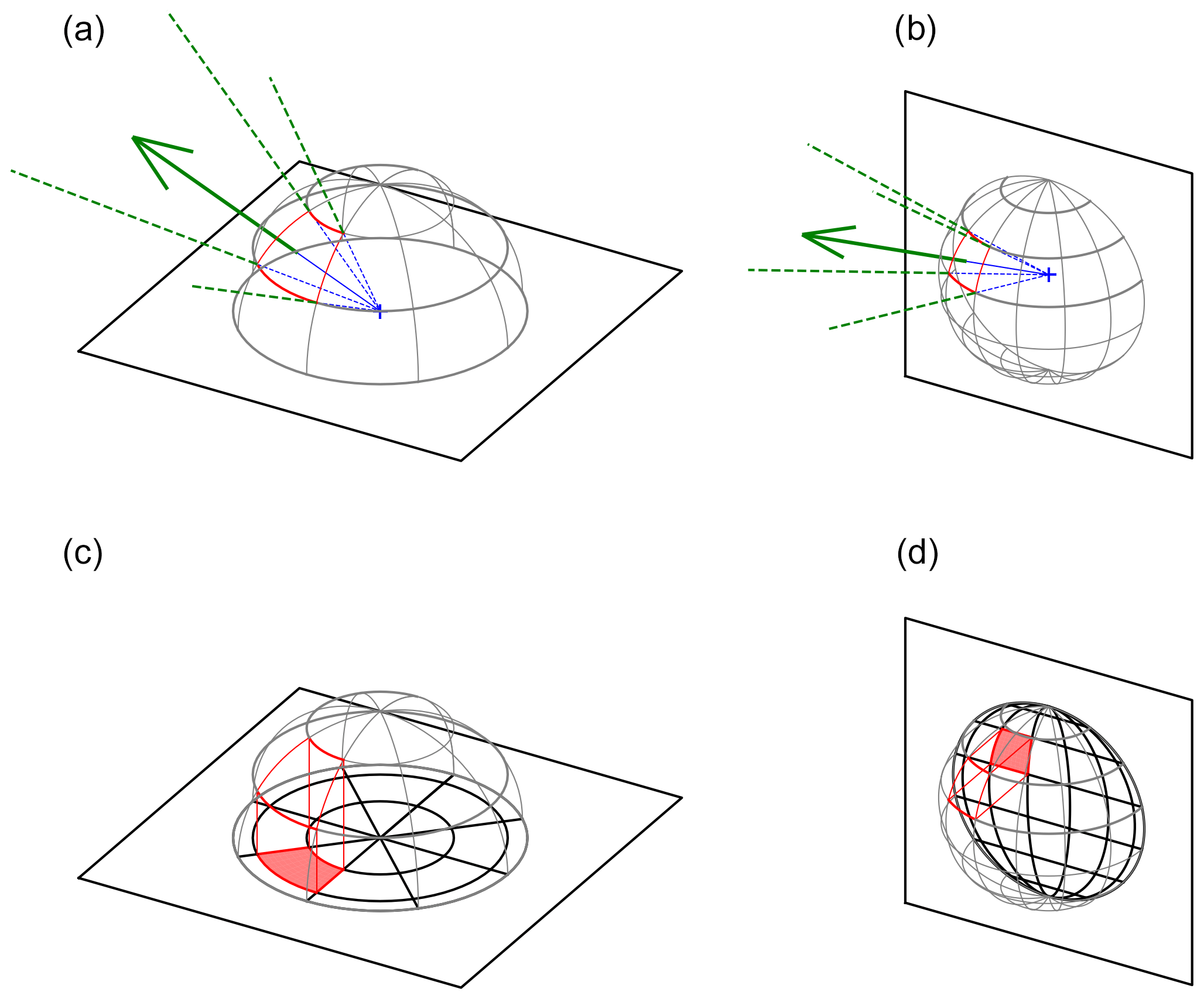
Figure 4A 3-D representation of the angular discretization scheme for a horizontal face (a, c) and a vertical face (b, d). The top panels depict a view from the centre of a horizontal and a vertical face; the view has been divided regularly by a fixed number of azimuth and zenith angles, as shown by the half-spheres. The green arrow indicates the traced ray representing the selected angular section, which passes through the centre of that section. The bottom row demonstrates the Nusselt analogue, whereby the area of each angular section's intersection with the half-sphere, as projected in the orthographic projection to the face's plane (solid red area), is directly proportional to the corresponding view factor value as a portion of the whole view. From the relative sizes of the projected areas it is clear that the view is less uniformly divided for the vertical faces, yet the unified discretization has computational benefits.
This approach is equivalent to the ray-tracing algorithm used in computer graphics; the only difference is that the ray directions in computer graphics correspond to individual pixels of the simulated camera's sensor and often some super-sampling is used for anti-aliasing. This similarity demonstrates that the result of this ray-tracing arrangement represents a reasonable simplification of view from the selected target and also that the accuracy can be improved as needed by increasing the angular resolution, i.e. the number of discretized azimuth and elevation angles.
An additional benefit of the angular discretization is the fact that the view factor values, if calculated analytically, always add up exactly to 1 and there is no need for normalization. A single face often represents an obstacle detected in more than one direction. In such cases, the respective view factors are aggregated to save resources. For faces very close to each other, the sum of the view factor values representing those directions is typically more precise than the normalized approximate value calculated using Eq. (5) just for the centres of the grid boxes.
2.2.5 View factor values for angular discretization
With angular discretization, the view from the centre of each face is divided into sections, each of which is bounded by azimuth angles [α0,α1] and zenith angles [θ0,θ1] (see Fig. 4). The portion of view represented by such a section is calculated analytically by integration.
The section of view between [α0,α1] and [θ0,θ1] can be viewed as an imaginary surface Aj on a unit sphere. The calculation of the view factor value is based on the view factor integral Eq. (2), where the sending surface Ai is replaced by the centre point Ci; therefore, the integral , which provides a spatial average over the surface Ai, is eliminated and only the integral over Aj remains:
Aj is a section of a sphere with centre Ci and radius r=1 limited by [α0,α1] and [θ0,θ1]. A ray from Ci towards a surface element is always perpendicular on it, giving . With this and , the view factor value equals
For a horizontal face, the normal angle is independent of the azimuth angle α and equal to the zenith angle θ:
In the case of a vertical face, the calculation depends on the orientation of the face. The calculation is presented for a northward-oriented face, for which the face normal . Considering the spherical triangle formed by the face normal, zenith and (α,θ), the central angle between the face normal and (α,θ) is calculated using the spherical law of cosines:
and the view factor value is
2.2.6 Computational complexity of the angular discretization
The angular discretization scheme greatly improves scalability, which can be demonstrated by following the two scaling approaches introduced in Sect. 2.2.2. In the case of angular discretization, the number of view factors and the memory requirements are limited by a fixed number for each face, and thus the asymptotic order of their growth is 𝒪(φ2) even in the case of increasing the resolution of the domain (the second case from Sect. 2.2.2).
The CPU time and interprocess communication demands for ray tracing are slightly higher than that because the average separation distance (i.e. ray-tracing length) grows with increasing resolution. For horizontal domain enlargement, only some ray-tracing directions will have greater distances, while for increasing resolution, all distances will be proportionally longer. In both cases, the demands are of the order of 𝒪(φ3) at worst, which is a great improvement from 𝒪(φ5). Furthermore, we have to consider that for any atmospheric model, the complexity of increasing resolution in the turbulent flow solver is between 𝒪(φ3) (considering only the increased resolution in three dimensions) and 𝒪(φ4) (also accounting for the shortened time step), so the radiative part can still theoretically scale better than the rest of the model.
2.3 Discretization of the direct and diffuse solar radiation
The direct and diffuse components of the incoming solar radiation and the thermal radiation from the sky towards surfaces are represented using the sky-view factor (SVF). It represents the portion of view from individual faces towards the sky which is not occupied by other faces. If the sky is viewed as an imaginary face, SVF makes the system of faces enclosed as specified in Eq. (1), which can be expressed as
The radiant fluxes from the sky propagate through the urban layer similarly to the reflected and emitted radiation from the faces with the exception that the source lies outside the urban layer. As the intention of the design is to avoid ray tracing during model time stepping for the reasons explained in Sect. 2.1, all ray tracing representing these rays is also done in advance during the initialization phase of the model just like with the other rays.
RTM version 3.0 represents the sky by a single SVF. The value of Fs is calculated by 2-D ray tracing as described in Sect. 3.1. For homogeneous diffuse solar radiation, this single value per face is sufficient to allow calculation of the diffuse solar irradiance. If the radiation inputs only provide total horizontal solar irradiance, this value is split into direct and diffuse components analytically (Boland et al., 2008). It is also possible to consider diffuse solar radiation to be inhomogeneous by splitting the sky into multiple regions and storing such separate partial SVF values per face because the number of regions would not increase with domain size; the current RTM code is ready for addition of this option once such radiation data are available.
When plant canopy simulation is disabled, the only information necessary to calculate the SVF for a specific location is the horizon height in each discretized azimuth direction, as described in detail in Sect. 3.1. When the semi-transparent plant canopy reduces transmittance from the sky (Sect. 2.4), the vertical structure of this partial shading is calculated in the means of angular discretization by adding a fixed number of discretized elevation angles for which the transmittance of the path from the sky towards the target face is calculated.
Direct solar radiation
The calculation of direct solar radiation during the model initialization phase is complicated by the fact that the apparent position of its source, the sun, and therefore the geometry of all rays, changes throughout the day, while all the other radiation sources in the model have fixed positions and geometries and only the values of their radiant fluxes change in time. RTM solves this problem by discretization of the apparent solar positions and performing ray tracing between these predetermined apparent solar positions and corresponding faces during the model initialization.
For a typical simulation which spans times of the order of hours or days, there is a fixed number of apparent solar positions (at most the number of radiation time steps), which is further reduced by discretization of azimuth and elevation angles using the nearest discretized direction. RTM uses the discretized directions that are already used for calculation of Fs in order to optimize the computation time and the memory requirements as much as possible.
For each discretized direction Dj and face i, the total ray transmittance is stored. This value is zero if there is an opaque obstacle (building or terrain) in that direction, i.e. if face i is fully shaded from direction Dj, and it is less than 1 if the ray intersects the semi-transparent plant canopy (Sect. 2.4). By multiplying by the current solar direct normal irradiance Ed and by the cosine of the incident angle, the approximate direct irradiance of face i is obtained:
where θi is the angle between the normal to face i and the exact value of the current apparent solar position.
2.4 Representing semi-transparent plant canopy
The resolved plant canopy in RTM is represented as a 3-D discretized field of leaf area density. RTM simulates the absorption of SW and LW radiation from the sun, the sky and modelled surfaces (i.e. shading by plants), as well as the thermal emission of LW radiation from the plant canopy towards the sky and the surfaces (see Fig. 1). The ray-tracing algorithm follows the ray from the source to the target and the attenuation is quantified for each PCGB that the ray intersects. Some other plant-canopy-related radiative processes are intentionally omitted for reasons of computational performance. These include the following.
-
Radiative interaction within plant canopy itself by means of LW radiation: interaction among individual PCGBs. This simplification has two reasons. The number of PCGBs can be much higher than the total number of faces in certain scenarios, generating huge numbers of mutually visible pairs of PCGBs, and it would be too complex to simulate it with the available computational resources – not to mention the complexity of including the sub-grid part of this interaction. On the other hand, if the LAD is high, then most LW interaction takes place between neighbouring PCGBs, and because the structure of air temperature is usually very smooth, such PCGBs have a low temperature difference, making the net exchanged radiative flux negligible; if the LAD is low, then its emitted LW flux density is also low.
-
Reflection in both parts of the radiation spectrum. The structure and arrangement of plant leaves allows for multiple reflections, but most of these reflections occur between leaves that are close to each other, which is mostly a sub-grid process (in typical resolutions of units of metres). Moreover, the high emissivity of leaves (and therefore low reflectivity according to Kirchhoff's law) makes their LW reflections negligible. The impact of SW reflection at nearby surfaces depends on the amount of reflected radiation in comparison to the background radiation from the same direction. The irradiation of the surfaces behind the plant canopy (further in the direction of the incoming radiation, e.g. below trees) is determined by the attenuation in the plant canopy (see Sect. 2.4.1 below), and if the LAD and extinction coefficient are appropriate, it is not significantly biased. The reflection and scattering by plant leaves towards other directions are disregarded by the current version of the model. This limitation needs to be taken into account while designing a simulation and considering the applicability of the model. The magnitude of the induced error and possible improvements of the treatment of SW reflection in plant canopy are a matter of ongoing research.
The main objects of radiative modelling in RTM are surfaces; the plant canopy is part of the process, but the focus remains on its interaction with surfaces. The data structures are organized accordingly and the ray-tracing algorithm is adapted to that as well. This arrangement allowed for the additional modelling of LW plant canopy emission and absorption into RTM with no data overhead and a negligible increase in computational time.
2.4.1 Calculating plant canopy sinks
This section describes the attenuation by the plant canopy of all the rays that are simulated by the ray-tracing algorithm – it applies to rays between faces, but also to the rays representing the diffuse and partially the direct solar radiation; the absorption of direct solar radiation is described in Sect. 2.4.3.
As the ray-tracing algorithm follows the ray from the source to the target, the attenuation is quantified for each PCGB that the ray intersects. Since the ray tracing is performed during the initialization phase of the simulation, the actual radiant flux carried by the ray is not yet known, but the attenuation can be expressed as the absorbed fraction of the flux that enters the PCGB. This fraction remains constant in time and independent of the absolute value of the radiant flux, as long as the leaf area density, on which the optical density of the plant canopy is based, remains constant. For this reason the RTM currently does not allow changing the LAD values during simulation time, which is usually not a problem for typical simulations lasting several days.
The plant canopy within the volume of each discrete PCGB is considered homogeneous, and the leaves are assumed to be randomly oriented. In reality the distribution of leaf orientation may be non-uniform, but this also depends on the tree species, the season, sun direction, and wind speed and direction. As some of these are non-constant during the simulation, and also the effect on absorption is less important than the distribution of LAD within the tree crown (Wang and Jarvis, 1990), RTM uses isotropic absorption inside the discrete PCGBs.
The ratio of the flux Φt passing through the grid box to the flux carried by the ray upon entering the box Φi is called transmittance (Tr), and it can be calculated as
where a is the leaf area density, s is the length of ray's intersection with the box (depending on relative angle and position) and α is the extinction coefficient, which converts LAD of trees and shrubs to a corresponding average optical density. The absorbed fraction Φa of the entering flux Φi is then calculated as . Equation (15) follows and extends the way the absorption of radiative flux in the plant canopy is calculated for the single-column case with aggregated leaf area index (LAI) in the PALM plant canopy module (PCM; see Maronga et al., 2015).
The exponential attenuation with respect to depth matches the Beer–Lambert law. As a continuous model of a discrete sub-grid process, it would correspond to an idealized case with non-transparent and non-reflective leaves wherein all leaves are homogeneously and randomly distributed in the volume of the grid cell; in that case, the only radiative flux passing through the cell would be the free rays that intersect no leaves. In reality, the transmittance of the tree crown is higher than that – the leaves themselves are semi-transparent and some further light is transmitted due to multiple reflections at the surfaces of the leaves. However, the attenuation with semi-transparent leaves is still exponential with respect to depth, and even the measured attenuation in homogeneous LAD media is close to exponential (Brown and Covey, 1966); therefore, a suitable extinction coefficient α can compensate for the fact that leaf transparency and reflectivity are not simulated explicitly, as was already assumed in the PALM PCM (Maronga et al., 2015).
For a ray that passes sequentially through PCGBs with transmittances , the total transmittance equals . The fraction of absorbed flux at grid box i divided by the total radiant flux Φr carried by the ray at its origin can be expressed as
This fraction, which will be further called the ray canopy sink factor (RCSF), is computed iteratively during the ray-tracing process, and it is stored for each intersection of a ray and a PCGB. The total transmittance Tr of the whole ray from the source to the target face is stored alongside the respective view factor, and the computed irradiance of the target face from that ray is always reduced accordingly.
The total flux carried by the ray from face j to face k is equal to
where Aj is the area of the source face j. The value of the absorbed flux can be obtained by multiplying this value by the RCSF. The flux absorbed at a PCGB does not depend on the ray's target, and only the total absorbed flux for each PCGB needs to be calculated:
Thanks to that, all RCSFs with the same source face and PCGB (i.e. those that differ only by the target face) can be aggregated. They are multiplied by the appropriate view factors, and the resulting sum is called the canopy-view factor (CVF):
This aggregation reduces storage and computation demands during the post-initialization time-stepping part of the simulation. The CVF only needs to be multiplied by the area of the source face and source face's radiosity in order to obtain the radiant flux absorbed by PCGB i originating from face j. A similar aggregation is used for calculating the absorbed radiative flux that originates from the diffuse solar radiation (see Sect. 3.1).
2.4.2 Thermal emission from the plant canopy
Modelling of the plant canopy thermal emission follows the concept outlined earlier. The emission from the plant canopy is considered from the target face's point of view, while the internal LW radiation exchange inside the plant canopy (among individual PCGBs and intra-grid exchange) is omitted.
Due to the reciprocity property of view factors, the CVF actually represents the fraction of view from face j that is covered by the plant canopy from PCGB i, taking into account the partial opacity, which is determined by the leaf area density in PCGB i. Consider the sub-grid semi-transparency to be caused by randomly distributed, small, fully opaque leaves with fully transparent gaps in between them; then, the CVF is exactly equal to the view factor from face j towards those leaves (i.e. their visible parts).
This enables straightforward modelling of the thermal emission originating from the leaves in PCGB i that is absorbed by the face j. Since reflection in the plant canopy is ignored, the emissivity of those leaves can be considered 1 according to Kirchhoff’s law, and using the Stefan–Boltzmann law, the emitted radiative flux from PCGB i in the direction of the face j is equal to
where Ti is the temperature of the air and leaves inside the PCGB i.
Thermal emission from the plant canopy towards the sky has to geometrically match the absorbed LW radiative flux from the sky in order to avoid biases in the total energy budget of the modelled domain. It is computed in a similar manner using the special CVF entries, which have the sky as the source instead of a face (their calculation is described later in Sect. 3.1).
2.4.3 Direct irradiation of the plant canopy
As described in Sect. 2.4.1, the canopy-view factors represent the partial absorption of radiation by the plant canopy only for the radiation that originates from surfaces and for the diffuse solar radiation and thermal emission from the sky directed towards the surfaces. The absorbed direct solar radiation, which accounts for the majority of absorbed radiative flux during clear-sky days, needs to be modelled separately.
In order to determine the direct radiative flux entering each PCGB with respect to shading by obstacles and partial shading by other PCGBs, RTM performs a separate ray-tracing procedure starting backwards from the centre of each PCGB towards the discretized apparent solar directions. For this ray-tracing process, no canopy-view factors are stored, and only the total ray transmittance is determined and stored for each PCGB k and discretized direction Dj.
During time stepping, the transmittance of the corresponding ray is multiplied by the direct normal solar irradiance Ed, which provides the radiative flux density entering PCGB k. The fraction of this flux which is absorbed by PCGB k is dependent on the dimensions of the PCGB, on the direction of irradiation and on the LAD of PCGB k.
RTM uses a sub-grid discretization model which sends an array of 60×60 parallel rays (organized to fill a bounding rectangle that contains the projection of the grid box) and calculates the transmittance of each of the rays using Eq. (15). These transmittances together produce an approximation of the fraction of absorbed flux divided by the flux density of direct normal irradiance. This fraction is calculated at the beginning of each time step using the known apparent solar position. Thanks to the fact that the grid is regular and the solar rays are parallel, this fraction is applicable to all PCGBs with a specified LAD. This simulation is performed with a single LAD value for all PCGBs m in the domain, and the result is linearized for all PCGBs using a factor . A technical description is available in Sect. S2.1 in the Supplement.
2.5 Calculation of mean radiant temperature
Mean radiant temperature (MRT) at a certain point in space is defined as the temperature of an imaginary object for which that object would be in radiative equilibrium with it surroundings, which means that the absorbed irradiance would be equal to the emitted radiant exitance. Calculation of the MRT is closely related to the radiative processes in the RTM, and thus it is implemented with advantage inside this module. This allows for the use of a similar approach and reuse of existing routines; it also ensures that MRT is calculated with the same discretization scheme as the scheme used in RTM for the calculation of LW and SW radiation, which allows users to avoid utilization of some highly simplified yet common approaches. Calculated MRT values are available directly in RTM in the form of PALM output variables, and they are provided to the biometeorology module for calculation of biometeorological quantities related to human thermal comfort (see Sect. 4.4).
Considering both LW and SW radiant fluxes for a hypothetical object with emissivity ε and SW albedo a, the MRT value TR can be derived from its defining equivalence and from the Stefan–Boltzmann law:
where ES is the average SW irradiance of the hypothetical object and EL is its average LW irradiance.
The calculation of the MRT utilizes a similar concept as the calculation of irradiance with angular discretization. For each point at which MRT would be simulated, the MRT factors are calculated during the initialization phase of the model run. MRT factors are the equivalent of the average irradiance factors for the whole surface of the hypothetical sphere, which means that there is no dependence on the direction of irradiance. For face i and MRT point j, the MRT factor is calculated as
where Aj is surface area of the sphere, is the angle between the connecting ray and the normal of face i, and is the length of the connecting ray. Equation (22) utilizes the fact that the ratio between surface of a sphere and its normal projected area (the area of a circle with the same diameter) is equal to 4.
The MRT factors are precalculated using the 2-D ray-tracing algorithm with angular discretization of the whole view, together with MRT sky-view factors and direct solar irradiance transmissivities for each MRT point. Depending on configuration, the MRT can be calculated for the centre of every grid box in the first layer above a terrain or even in multiple vertical layers.
The pure physical MRT value is usually defined with respect to a spherical black-globe thermometer. On the other hand, the biometeorology applications require the MRT value related to a clothed human body, which is tall and narrow, and it is therefore affected by radiation from its sides proportionally more than by radiation directly from above. It is modelled in RTM as a configurable asymmetrical generic object with specified albedo, emissivity and aspect ratio. These MRT values for the hypothetical human body are then provided to the biometeorology module. Further details are described in Sect. 4.4.
The basic ray-tracing algorithm, which is used in RTM when the legacy discretization of view is enabled, was first implemented in RTM 1.0 as part of PALM-USM 1.0, and is it carried over from previous versions of RTM with minor changes like the addition of options Fmin and smax to reduce the number of view factors (see Sect. 2.2.3) and adaptations to changes in other parts of RTM. Its current implementation in RTM 3.0 is described in Sect. S1.1.
3.1 Azimuthal ray-tracing algorithm
With the introduction of the angular discretization in RTM version 2.0, a new variant of the ray-tracing algorithm was developed, which was highly optimized for this angular discretization. This algorithm is further called 2-D ray tracing.
This is a novel algorithm which takes significant advantage of the specific data representation and parallelization of the PALM model. The 3-D fields in PALM are represented as arrays for which the z dimension is the fastest changing; therefore, vertical columns are memory-contiguous and quickly loaded. Moreover, the 2.5-D geometry enables such a representation of surfaces that allows fast access to all surfaces with a specific horizontal coordinate. Finally, the MPI parallelization of the PALM model splits the domain horizontally into individual subdomains, therefore each vertical column is contained within one subdomain and nearby columns have a high probability of being in the same subdomain.
The algorithm utilizes the following feature of the 2.5-D geometry: for every point of view and for every azimuth there is a distinct horizon (γ), i.e. the elevation angle below which the view is completely obstructed by terrain and/or buildings and above which there is only sky. The extension of this algorithm to a full 3-D geometry is discussed in Sect. 6.
The core of the 2-D ray-tracing algorithm works by following a discrete set of azimuths from point (representing the centre of the target face) in the direction of the azimuth until it reaches the horizontal domain border. For each azimuth it tracks the monotonically increasing horizon angle; more specifically, it tracks , where represents coordinates of the obstacle representing the tracked highest horizon angle. The tracking itself works just like the basic ray-tracing algorithm (Sect. 1.1) except in just two dimensions – one step means one vertical column for which the terrain and building height is compared against the currently known horizon.
To determine partial shading by the plant canopy, RTM needs to track more than just the horizon angle for each traced azimuth. The plant canopy may have a diverse vertical structure; thus, an evenly discretized set of elevation (zenith) angles is tracked for each azimuth. This forms a uniform, regular set of directions, which is used for all types of radiative processes; it is used for calculation of the sky-view factors, direct irradiance transmittance and also for the angularly discretized view factors towards other surfaces. This way, a single 2-D ray-tracing routine computes all the respective values at once without any overhead.
During tracing of each ray, the information about LAD all along the ray path is needed. This information is distributed in particular MPI processes and needs to be obtained by means of MPI communication. In order to reduce fragmentation of one-sided MPI operations, the 2-D ray tracing requests all LAD data for all applicable PCGBs belonging to the whole half-plane cross section (one discrete azimuth) in all required vertical levels at once. When these data are retrieved from all involved MPI processes, the RCSFs are generated in a two-pass calculation for each discrete azimuth – from point towards the horizon and then back. Both of these directions are necessary: one for the absorbed fraction of incoming diffuse radiation from the sky and the other one for the absorbed fraction of the outgoing (reflected and emitted) radiative flux towards the sky. In addition to that, the total transmittance of each ray is saved. The generated RCSFs are sorted and aggregated continuously; after all ray tracing is done, they are redistributed among processes using MPI alltoallv similarly as with the basic ray-tracing algorithm.
The 2-D ray-tracing algorithm needs to determine the complete information for the time-stepping radiation calculation, including the index of the opposing face, the view factor value and the total transmittance of the connecting ray, for each discrete direction under the horizon angle. As specified in Sect. 2.2.4, the view factor value is determined solely by the regularly discretized fraction of view. For vertical faces, it is calculated using Eq. (12), where α0 and α1 are the midpoints between the calculated discrete azimuth and the neighbouring discrete azimuths (or or , where the calculated discrete zenith angle is the first or the last value, respectively), and θ0 and θ1 are the midpoints between the calculated discrete zenith angle and the neighbouring discrete zenith angles (or 0 or π as boundaries). For horizontal faces, a similar approach is used with Eq. (10).
The index of the opposing face has to be determined using MPI one-sided communication request (MPI get) because the array with reverse indices (xi, yi, zi, di) →i (where di is the face orientation – northward, eastward, southward, westward or upward) is once again a 3-D array for which each process can only hold its own subdomain in its local memory, as the array for the whole domain would be too large.
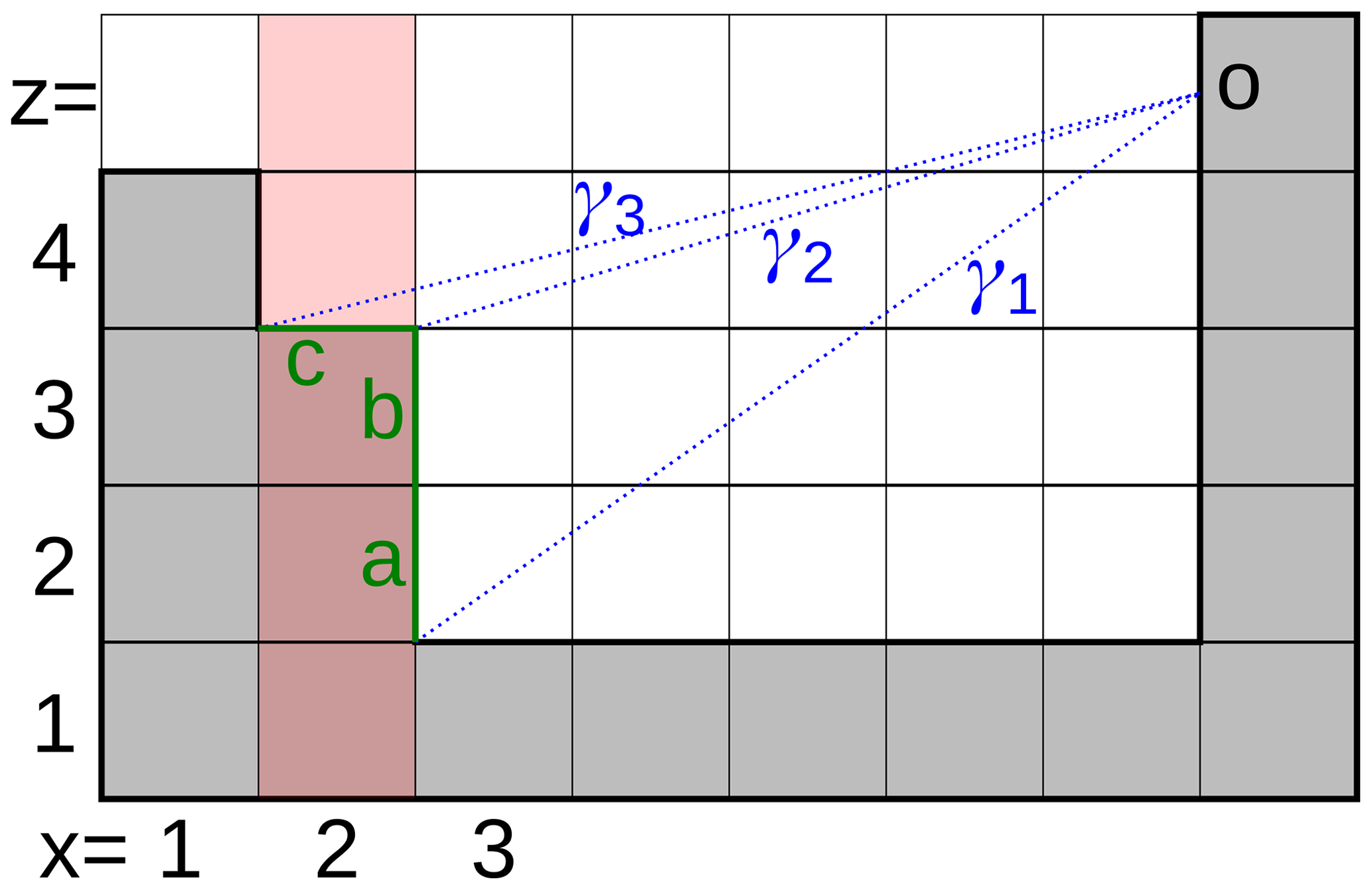
For each new grid column processed during ray tracing, there may be at most one new horizontal face and zero or more vertical faces identified as new opposing faces. The identification algorithm can be demonstrated with an example shown in Fig. 5. The ray-tracing procedure, originating from face o which progresses in the azimuth direction corresponding to the cross section in the figure, enters column x=2 with the current horizon angle γ1, which was the result of column x=3 having terrain height z=1.5. The column x=2 has terrain height z=3.5, which yields two new horizon angles γ2 and γ3 for entry to the column (x=2.5) and exit from the column (x=1.5), respectively. Because γ2>γ1, there will be new vertical opposing faces for each discretized ray between , in this case faces a and b. The orientation of these faces is determined by the fact that the boundary between columns was decreasing in dimension x; i.e. they are eastward-oriented faces. Furthermore, because γ3>γ2, as long as there is at least one discretized ray between , there will also be a new opposing horizontal face c.
The generated VF entries for the opposing faces are sorted and aggregated for each ray-tracing origin (after ray tracing towards all discretized azimuth angles), creating at most a fixed number of entries that do not need to be normalized, as described in Sect. 2.2.4. VF entries are always generated in the process of computing the subdomain where the target face lies; therefore, there is no need for their redistribution.
3.2 Radiation processing in time stepping
RTM radiation interaction is called in PALM after every call of the one-column radiation scheme (e.g. RRTMG), which is applied in regular configurable intervals. For each radiation step, the radiative fluxes on the top of the urban canopy layer are updated first, and then the RTM calculates the fluxes within the urban layer using inputs from its top border.
The implementation of the time-stepping part of RTM is straightforward, and its changes since RTM 1.0 are only related to the addition of newly simulated processes, like the plant canopy LW interaction and the calculation of MRT. The current implementation in RTM 3.0 is fully described in Sect. S1.2.
This section presents the parts of the RTM module that are responsible for interaction with other modules in PALM, together with the respective parts in those modules that were added by the authors of this paper in order to enable the coupled simulation of the described processes.
4.1 Radiation forcing model
As described in Sect. 1.2, the RTM simulates radiative fluxes inside the urban canopy layer by taking the radiation fluxes from the PALM one-column radiation model as input. As the result of this simulation, RTM calculates the radiation reflected from the surface to the atmosphere more realistically than the one-column model. In order to take advantage of that, the RTM results need to be considered back in the forcing radiation model. This forms a two-way coupling between the forcing radiation model and RTM. This section describes the implementation of the second backward direction of this coupling and follows one of the possible approaches used in mesoscale models (Schubert et al., 2012).
The implementation is based on calculating effective radiation surface parameters for the radiation model: an effective surface emissivity ϵeff, surface temperature Teff and urban albedo αeff. These parameters are calculated so that they would, when applied to a simple single surface as assumed in the forcing one-column radiation model, give similar radiation fluxes as the complex 3-D urban area.
For LW radiation, the lower boundary condition of the forcing radiation model can be expressed as
where L↑ is the upwelling LW radiation, which represents the total radiation emitted and reflected into the sky from the urban surfaces as calculated by the RTM. The downwelling LW radiation L↓ is provided by the forcing radiation model as an input to the RTM.
Here, ϵeff is selected as the average of the surface emissivities ϵi of the surface i over the area Ai:
With that, only L↑ is needed to calculate Teff with Eq. (23). The straightforward way would be to sum up the emitted and reflected radiation from each surface, taking into account the corresponding sky-view factor. For efficiency reasons, the energy conservation for the total urban area is used instead:
The terms on the left-hand side represent the total energy input from the sky and the total LW emission of the urban surfaces. The right-hand side stands for the total absorbed energy by the urban surfaces as well as the total energy emitted and reflected to the sky. This can be combined with Eq. (23), yielding
where
Here, is the radiation received by a surface with temperature Ti from the sky, and Li is the respective total received LW radiation including reflections and LW emission from other surfaces.
The standard choice that the normalizing area Anorm represents the horizontal modelling domain size with domain size lx and ly in the x and y direction, respectively, does not work here. In order to receive a realistic amount of diffuse radiation from the sky, it is necessary to consider not only radiation from the sky area of size Ahoriz above the modelling domain but also radiation from the side areas of the domain. In general, however, this leads to , which is not unrealistic because higher (lower) received radiation within the domain would be compensated for by lower (higher) received radiation outside the domain. To tackle this issue, the approach is to receive L↓ from the sky but with a different reference area Anorm calculated as
For SW radiation, the lower boundary condition of the forcing radiation model can be expressed as
with the downwelling SW radiation K↓ as calculated by the forcing radiation model and the total upwelling SW radiation K↑. Expressing K↑ in terms of absorbed SW radiation Kabs with
yields
where
Here, is the SW radiation from the sky received by surface i with albedo αi and Ki is the total SW radiation received by the respective area including reflections from other surfaces.
4.2 Building and land surface models
Radiative transfer between the atmosphere and surfaces as well as among surfaces themselves depends on the surface temperature, which is the result of the surface energy balance calculated in the surface modules. However, one of the components in the surface energy balance is the surface net radiation, which is calculated in the RTM. The exchange of information between the surface modules and the RTM is therefore mutual.
PALM includes two surface modules: the land surface module (LSM) for natural-like surfaces, such as vegetation-covered, water and pavement surfaces, and the building surface module (BSM) for building surfaces such as walls, windows and roofs. Both modules solve the energy balance for each surface, partitioning the available net radiation into ground–wall heat fluxes, as well as sensible and latent heat fluxes. For a detailed description of LSM and BSM see Maronga et al. (2020).
Each of the discrete surfaces may have distinct soil or wall material properties, such as heat capacity or conductivity, as well as distinct surface properties such as albedo, thermal emissivity and roughness length. In the LSM a face (i.e. surface element in LSM and BSM terminology) is assumed to be either vegetation, water or pavement, while in the BSM a surface element is further divided fractionally into walls, windows and green surfaces. Each fraction exhibits distinct radiative properties. For performance optimization reasons, the corresponding properties and state variables for the surfaces are stored within a dynamic data structure, which encompasses arrays for various surface variables. Each type of surface with different a spherical orientation has its own derived data structure defined; e.g. northward- and southward-facing BSM surfaces can be accessed individually without further if–else conditions necessary. This way of representing the surface allows for the execution of surface-energy-related code in a consecutive manner without hampering loop vectorization. However, RTM solves interactions between all surfaces and it thus needs, again for optimization reasons, one single array of surface properties and state variables. Hence, surface information from the respective arrays of the derived data structure is gathered into a single linear array before the RTM code is executed. This is done for the surface temperature, albedo and emissivity. For fractional surfaces, these values are calculated as the weighted average of the different fractions (wall, window and green fractions).
After the radiation interactions are performed in the RTM, the resulting LW and SW radiation fluxes at the surfaces are distributed back onto the surface-type data structure. Subsequently, the updated radiation fluxes at the surfaces are supplied to LSM and BSM.
4.3 Evapotranspiration and latent heat in plant canopy model
An important process associated with plant canopies is transpiration of water vapour from the green parts of plants. It is actively controlled by plants by opening and closing stomata and thus changing the resistance of the leaf surface against the evaporation of the leaf water. This process is mainly affected by the incoming SW radiation, air temperature, air humidity and the soil water content (e.g. Stewart, 1988; Daudet et al., 1999). The explicit 3-D simulation of SW radiation in RTM allows for the creation of the transpiration model for the resolved plant canopy within the 3-D grid of the model. This enables explicit interactions within the model resolution, such as partial shading in the LAD structure within a tree crown based on directions of incoming radiation from multiple sources. The transpiration model calculates humidity gradients and latent heat fluxes, completing the description of the atmospheric thermal energy processes in the plant canopy.
Calculation of the plant canopy transpiration rate is based on the Jarvis–Stewart model in the form described in Daudet et al. (1999) and Ngao et al. (2017). Namely, the evaporation rate from the leaf surface Er is computed as
where Eeq is the equilibrium evaporation per leaf unit area, Eimp is the imposed evaporation per leaf unit area and Ω is the decoupling factor. These variables are modelled as
where Rn is the net radiation provided by the RTM for each PCGB, is the water vapour pressure deficit in the air (with es and e being the water vapour pressure at saturation and the water vapour pressure, respectively), is the partial derivative of the water vapour saturation pressure with respect to temperature, is the psychrometric constant, gb is the leaf boundary-layer conductance and gs is the stomatal conductance. The stomatal conductance is computed as
where gs,max is an empirical maximum conductivity value and are empirical functions, which depend on the incident SW radiation, the temperature, the water pressure deficit and the residual soil water content (RSWC) (Van Wijk et al., 2000). The empirical functions are adapted from Stewart (1988) and Van Wijk et al. (2000).
The resulting latent heat fluxes and humidity gradients then enter the prognostic equations of humidity and potential temperature (see Eqs. 3 and 4 in Maronga et al., 2020) as additional sources terms.
4.4 Biometeorology module
The biometeorology module in PALM (BIO; see Fröhlich and Matzarakis, 2019) provides spatial and temporal information on human thermal comfort. This is expressed in the form of biometeorology indices, such as physiologically equivalent temperature (PET), universal thermal climate index (UTCI) and perceived temperature (PT). All these indices require the mean radiant temperature (MRT) with respect to a simulated human body.
The calculation of MRT is closely related to the RTM radiative processes. This fact allows for the calculation of MRT inside RTM with little additional effort and overhead utilizing the existing RTM routines (see Sect. 2.5). It also ensures that MRT is simulated similarly to other radiative fluxes (i.e. using the same discretization and numerical methods), which allows users to avoid substantial simplifications often used in other models (a review is in e.g. Fröhlich and Matzarakis, 2019). However, this approach requires the interconnection and collaboration of the RTM and BIO modules.
The RTM provides the MRT values for the BIO module in the form of separate SW and LW mean irradiance for each simulated MRT box. This approach allows the BIO module to process the incoming fluxes independently and to apply the radiative properties of the human body (albedo and emissivity) inside the BIO module. The shape of the simulated body, however, affects the MRT factors, and thus it needs to be defined inside the RTM. The current version of RTM contains three selectable types of MRT body geometries: sphere (simulated globe thermometer), ellipsoid and a simple human body parameterization, with the possibility to supplement other arbitrary geometries. The ratio of the major and minor axes of the elongated shapes is configurable in RTM with the default of 7.3. More details about the currently implemented shapes are available in Geletič et al. (2021).
This section presents an evaluation of the convergence and computational performance of the current RTM implementation. A validation of the whole PALM model with RTM in a realistic urban environment against a comprehensive set of observations for a large scenario in Prague–Dejvice is presented by Resler et al. (2020). There are also further validation studies (e.g. Berlin) in preparation. A detailed study on the relative importance of individual radiative transfer processes is presented in Salim et al. (2020). Tests of the sensitivity of the PALM model to specific RTM input parameters are included in Belda et al. (2020).
The simulations presented in Sect. 5.1, 5.2, 5.3, 5.4 and 5.5 are based on a small urban scenario in the Prague–Holešovice crossroads of Dejvická and Komunardů streets, similar to the tiled base scenario used for the sensitivity study in Belda et al. (2020), which itself is based on the scenario used for validation of the PALM-USM model (Resler et al., 2017).
5.1 Convergence with respect to model resolution
The surface geometry and properties used in RTM are available with a certain level of detail and discretized by a regular grid. Hence, a natural expectation would be that decreasing the grid spacing below a certain level would not introduce new information and that the RTM would converge to one solution. With RTM, increased model resolution leads to a higher number of finer faces and PCGBs. In order to investigate how sensitive the resulting radiative fluxes are to model resolution, multiple simulations have been performed for the small urban scenario with resolution halved iteratively from 8 m down to 0.5 m. Because only radiative fluxes are of concern in this experiment, only one daytime time step was compared.
The finest simulation with a resolution of 0.5 m is taken as the base case, and other scenarios are compared to it by radiative fluxes at the matching surfaces. Finer resolutions mean increased detail in the 3-D structure of model surfaces; therefore, not all surfaces represented in the finer-resolution scenario correspond to the coarser-resolution scenario. In this experiment, around 70 %–80 % of fine-resolution faces could be matched to respective coarse-resolution faces. The results are shown in Fig. 6.
On double-logarithmic scales the radiant flux errors decrease almost linearly. The largest errors can be observed in the SW fluxes, with deviations to the reference case of almost 100 W m2, while errors in the LW fluxes are smaller by about 1 order of magnitude. Extrapolating to even finer spatial resolution would imply that the mean error made for the LW fluxes becomes negligible, while the mean error for SW fluxes is still of the order of a few Watts per square metre (W m−2). However, we emphasize that this is not related to the RTM itself but to the edged representation of sloped surface geometry on the Cartesian grid, which successively approaches the “real-world” surface geometry with increasing spatial model resolution so that mutual surface reflections become more realistic.
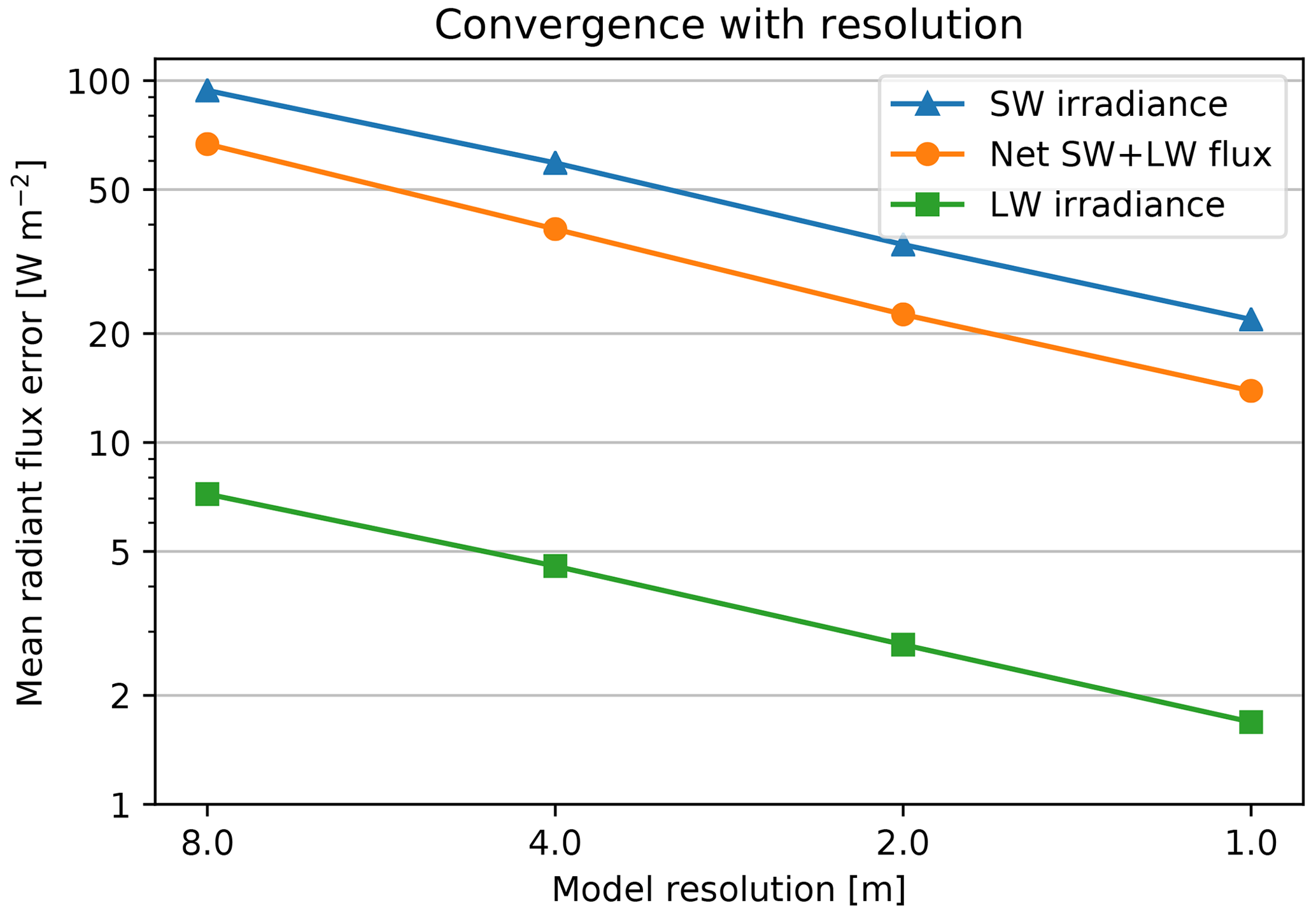
Figure 6Double-logarithmic presentation of mean deviations of surface SW and LW irradiance as well as net radiant flux against the finest-resolution case of 0.5 m.
5.2 Convergence of angular discretization
The angular resolution of the angular discretization scheme (see Sect. 2.2.4) can be controlled by setting the number of horizontal (azimuth) and vertical (elevation) directions. The default values are 80 and 40 steps respectively, i.e. 4.5∘ steps. This section explores the convergence of increasing angular resolution on the small urban scenario.
The angular discretization resolution also controls the discretization of direct solar irradiance; therefore, different angular resolutions also lead to a different number of discrete apparent solar positions throughout the day. For this experiment, a 1 d long simulation was performed with five different angular resolutions: 18∘, 9∘, 4.5∘, 2.25∘ and 1.125∘.
Table 1 lists parameters of the experiment. With doubling the angular resolution the number of discrete directions quadruples, while the number of view factors grows more slowly. This is a result of the aggregation of view factors with an identical source and target face in the angular discretization scheme, as the increased angular resolution would surpass grid spacing for increasingly distant mutually visible surfaces. For the target faces for which the angular resolution is already finer than the grid spacing of the faces in its point of view, the increased number of rays traced from each visible face brings improved precision of the VF values without increasing the number of VFs.
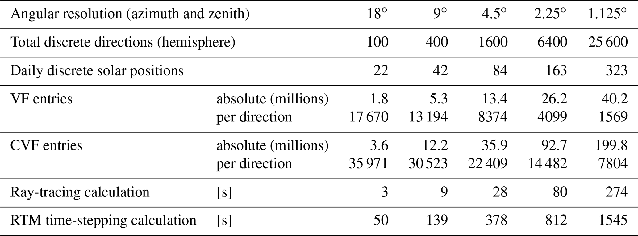
The results for the convergence are shown in Fig. 7, which shows mean absolute differences relative to the reference case with the finest angular resolution (1.125∘) for the selected radiative fluxes for each face throughout the 24 h long experiment. On double-logarithmic scales the mean deviation in the radiative fluxes are almost linear, with the largest deviation again observed in the SW fluxes. However, compared to the grid resolution, the error made by an overly coarse angular discretization is significantly smaller. Although increasing the angular resolution has relatively low demands on computational resources in comparison to increasing the spatial resolution of the model, the default value of 4.5∘ provides a reasonable trade-off.
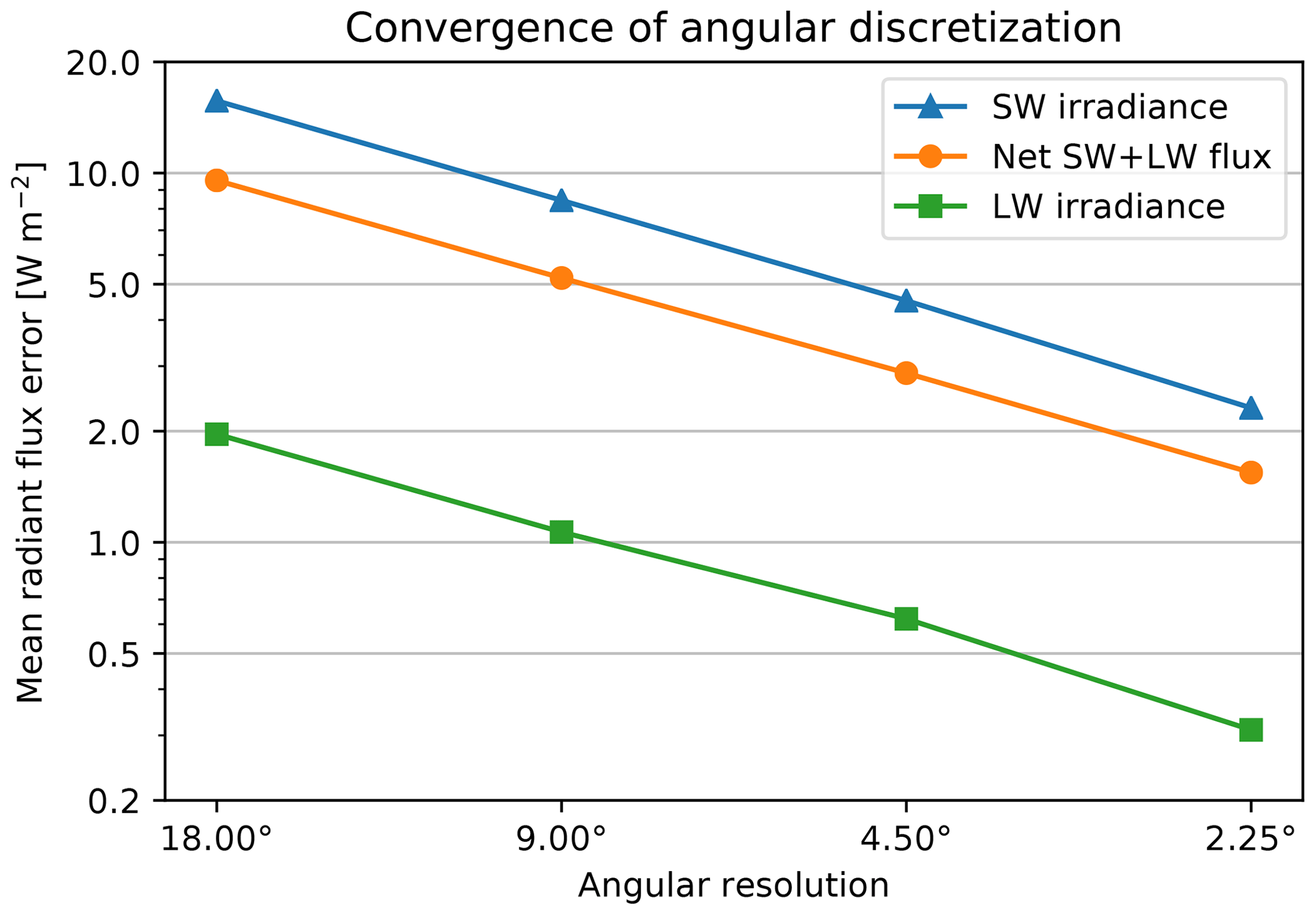
Figure 7Double-logarithmic presentation of mean deviations of surface SW and LW irradiance as well as net radiant flux for different angular resolutions. Mean deviations are shown relative to the finest angular resolution of 1.125∘.
5.3 Convergence of multiple reflections
In order to quantify the appropriate number of reflections for typical urban scenarios, a simulation of the small urban scenario was performed for one time step of a summer daytime simulation with a different number of reflection steps. To evaluate deviations in net radiant flux values, the reference scenario was simulated with an excessive 300 reflection steps, for which all remaining unreflected flux values are almost zero, i.e. below the lowest positive value of the floating-point numerical representation.
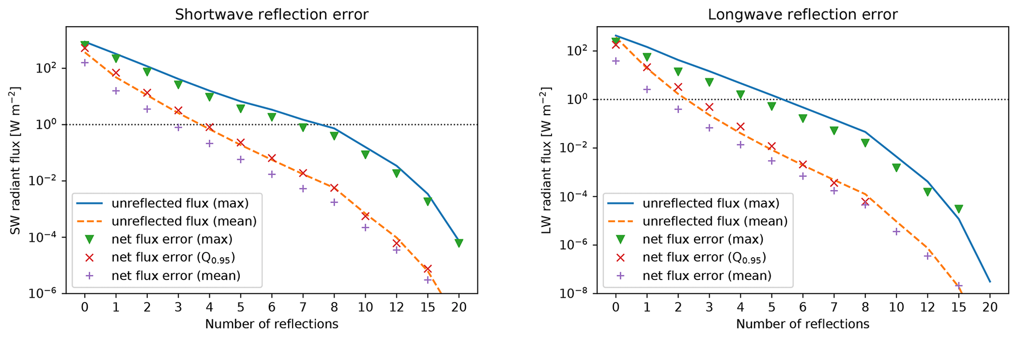
Figure 8A double-logarithmic presentation of potential and actual errors in SW and LW radiation caused by an insufficient number of reflections. The maximum and mean of the remainder of unreflected radiation per surface are shown as lines; the absolute discrepancies of net radiant flux compared to a perfectly reflected scenario are shown by individual points (maximum, 95th percentile and mean). The net flux errors above 15 reflections are zero (below the floating-point resolution), and so are the 95th percentiles of LW error above 8 reflections.
The results are shown in Fig. 8. For SW radiation, the mean net radiant flux error is below 1 W m−2 after three reflections, and the 95 % quantile of the net flux error and the mean unreflected radiant flux are below 1 W m−2 after four reflections. For LW radiation, which reflects less in typical scenarios, these respective limits are reached one reflection earlier.
These results support the recommendation to use the default RTM configuration value of three reflection steps for most scenarios. Considering that with the default radiation update interval of 60 s, the RTM uses only a small fraction of time-stepping computational time, the number of reflection steps can be increased to e.g. five with negligible computational costs.
5.4 Model scalability in large scenarios
To verify model scalability, a horizontal scaling experiment was performed on the Salomon supercomputer at IT4Innovations National Supercomputing Centre3. The experiment was based on the small urban scenario of Prague–Holešovice.
The original model domain was doubled iteratively in both the x and y direction, creating a tiled scenario with 2n rows and 2n columns (22n copies) of the original domain for . Each scenario was simulated using a proportional number of parallel processes, having 32 processes per tile and the total number quadrupling with each iteration. The Salomon supercomputer is composed of individual nodes with 24 CPU cores per node interconnected using the InfiniBand FDR fabric; therefore, the scaling test used multiple nodes, also testing the scalability of remote data exchange.
For each domain size, a short 10 min simulation was performed, and the durations of individual tasks from model initialization and model time stepping were recorded together with the number of view factor data entries as a measure of memory complexity. The radiation update interval was 60 s.
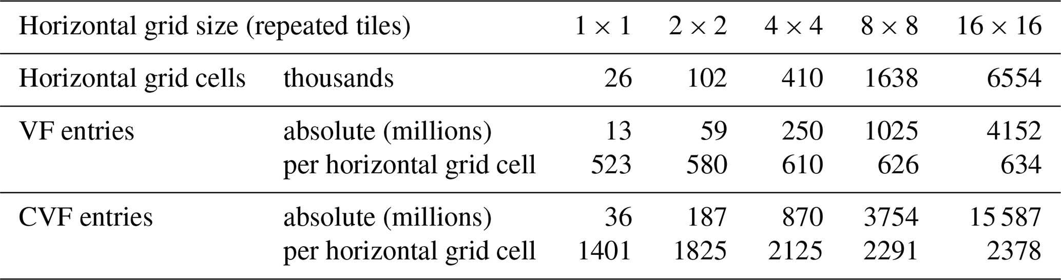
Table 2 lists the number of view factor entries for the horizontally tiled domains. Thanks to the constant maximum number of view factor entries in the angular discretization scheme, the actual number of entries per horizontal grid cell grows only slightly due to mutual visibility among the tiles, allowing less aggregation in more complex scenarios. The number of plant canopy-view factor entries per face could grow proportionally to the mean ray length in the worst case, but the real case shows that, due to shading, the actual number of entries per face only increases moderately with exponentially larger domains.
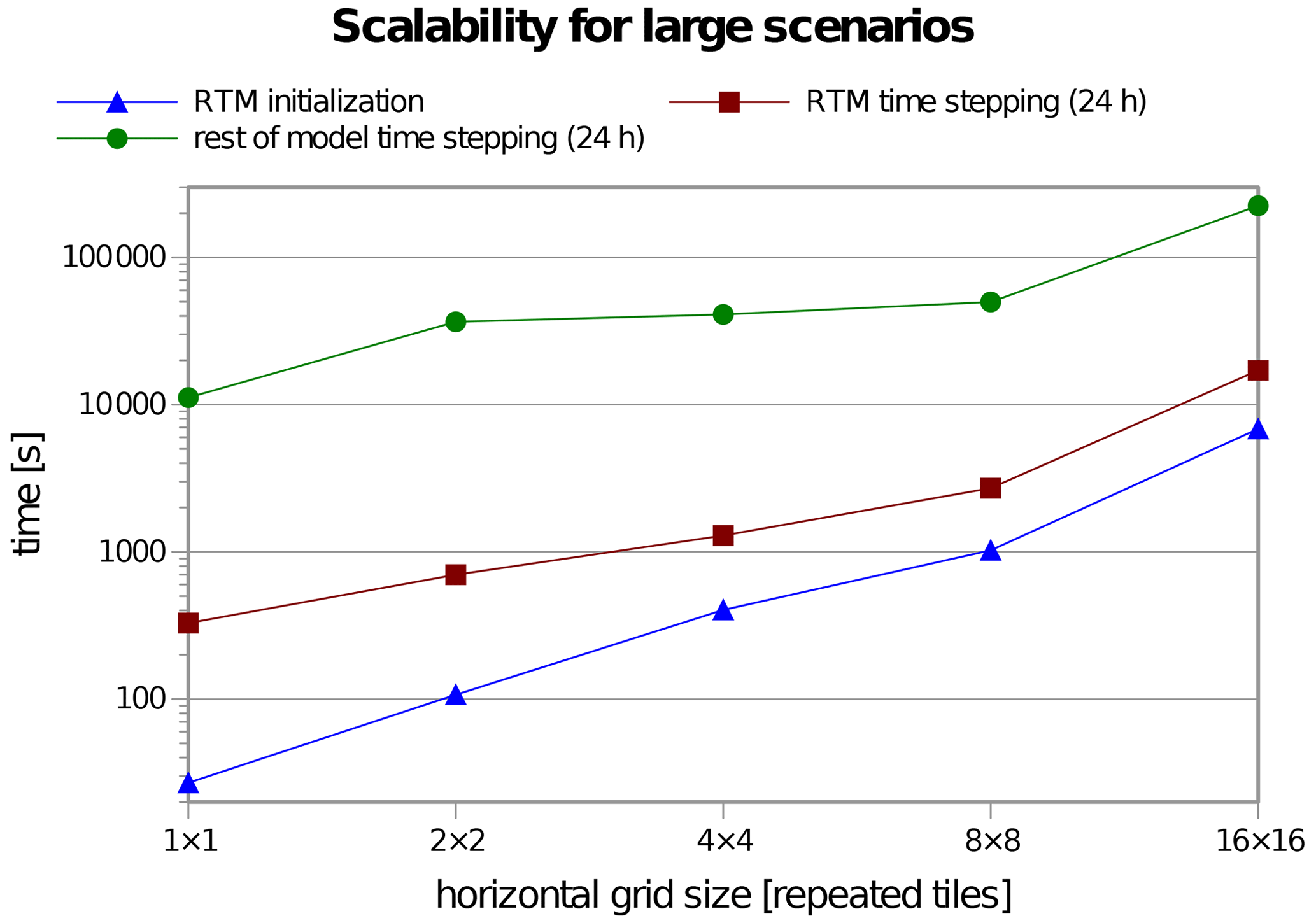
Figure 9A double-logarithmic presentation of the computation time spent for different sub-tasks while simulating progressively larger domains (by the means of horizontal quadruplication). Each simulation uses a constant number of processes per horizontal tile. The sub-tasks shown are RTM initialization and time stepping along with time stepping of the rest of the model as a reference. Time-stepping time is shown for a 1 d long simulation as extrapolated from the 10 min test simulations.
The computational time measured by the scalability test is presented in Fig. 9, split into the initialization phase (which is independent of the length of the simulation) and the actual time-stepping phase. As can be seen in the log–log plot, the RTM initialization time (ray tracing and data aggregation) is mostly proportional to the horizontal domain size, as expected from the increase in ray-tracing lengths and the amount of interprocess data exchange (see theoretical complexity in Sect. 3.1). Ray tracing is the most data-exchange-intensive process in model initialization.
The temporal scaling of the time-stepping phase of RTM is shown together with the time stepping of the rest of the model as a reference. RTM calculation takes between 2 %–5 % of the time-stepping phase. The largest simulated domain with 8192 parallel processes running on 342 individual nodes displays slight worsening of the scaling curve for both RTM and for the rest of the model, probably due to the growing complexity of interprocess data exchange. Future versions of RTM may be improved for the largest domains thanks to planned optimization of the amount of exchanged radiative flux data (see Sect. 6).
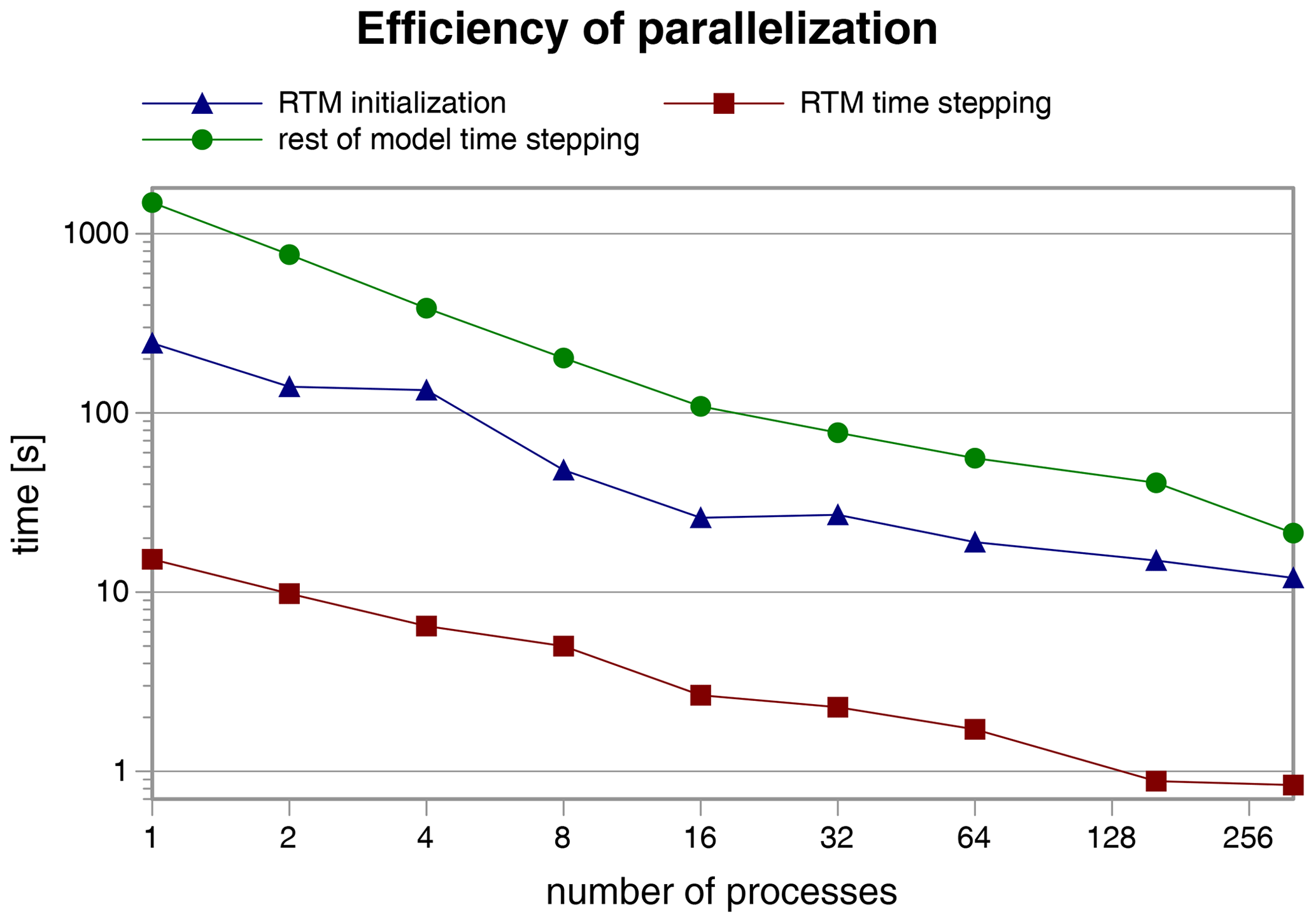
Figure 10A double-logarithmic presentation of computational time versus the number of processes for a small scenario, typically suitable for 16–32 processes.
5.5 Efficiency of parallelization
Figure 10 shows the efficiency of parallelization for a small domain composed of a single tile of the scaling test domain. A domain of this size should be computed with up to 64 processors for reasonable simulation times, yet we explore an approximately exponential sequence starting with 1 process up to 320 processes, at which point each subdomain has only 10×8 horizontal grid cells.
We can see that between 1–16 processes the parallelization of both the initialization and time-stepping phases is very good, even though the radiative interactions have very strong spatial interdependency, meaning significant mutual data exchange between subdomains. For further increasing the number of processes, both the RTM initialization and the RTM time stepping become less efficient. This is attributed to the relative increase in costs for MPI communication compared to the cost of computations performed on each process, which is in accordance with Amdahl's law of strong scaling. In other words, when the subdomains become too small the speed-up with an increasing number of processes becomes less efficient.
5.6 Performance in a large realistic urban scenario
Resler et al. (2020) focus on validation of the PALM model on a large urban scenario, which is composed of two nested domains. The outer domain covers an area of 4 km × 4 km with a resolution of 10 m, and the inner domain has an extent of 1440 m × 1440 m and a resolution of 2 m. An example of the simulated radiation for the inner domain is shown in Fig. 11. The simulation was performed on a cluster with Infiniband EDR interconnection on 880 MPI processes. In this simulation, the RTM initialization took 10 min, and within the 72 h time stepping, the RTM calculation took between 0.5 % and 1.5 % of the time of computation depending on meteorological conditions.

Figure 11A 3-D representation of instantaneous net SW + LW radiative fluxes in a large urban scenario. A north-oriented view of the inner domain of the Prague–Dejvice validation scenario.
This paper gives a description of the significantly updated and extended model RTM 3.0 in PALM. It focuses on new and redesigned features in comparison with RTM 1.0, which was described in Resler et al. (2017). Several of the presented methods and algorithms, namely the angular discretization method (Sect. 2.2.4) and the 2-D ray-tracing algorithm (Sect. 3.1), are novel in the field of microscale atmospheric modelling. All the new features of the model have been designed and implemented as fully integrated in the PALM model, taking into account the specific features and properties of the atmospheric model.
Also, sensitivity tests on performance-affecting configuration options (spatial model resolution, resolution of angular discretization and the number of reflection steps) are presented in this study, supporting their recommended configuration for typical urban scenarios. Finally, the applicability of RTM to large real-life scenarios is presented, demonstrating that the computational demands of RTM are in line with other components of the PALM model with respect to domain size.
Outlook
Model validation on large scenarios and long-term experience with various realistic simulations have also identified specific weak points in model representativity and RTM's potential for further improvements (see Resler et al., 2020). New or improved simulated processes, different representation of model elements, and possibilities for further improvements in computational efficiency and scalability are all included in upcoming development plans for the RTM.
Fully three-dimensional buildings
Several modules in the PALM model, as well as the model core, now support fully 3-D structures with downward-facing faces e.g. at bridges or lateral openings to courtyards. However, in many real-world scenarios overhanging structures are infrequent and only occur at a minor number of grid points. The current ray-tracing algorithms takes advantage of the 2.5-D geometry to improve computational efficiency. Hence, the proposed update will still use the simplifications made for the 2.5-D geometry while enabling the fully 3-D support only at grid points where required.4
Immersed boundary method
For now, the representation of obstacles in PALM is fully based on the Cartesian grid; i.e. a grid box is either fully obstacle or fully atmosphere. As a consequence, surfaces that are actually slanted in reality, such as roofs and natural slopes, are represented as step-like surfaces. Beside implications for microscale flow biasing e.g. the surface friction, such step-like representation increases the total surface area in the model, which affects the amount of radiative flux and adds artificial shading and reflections. Future developments of PALM include the implementation of the immersed boundary method (IBM) (Peskin, 1972) that also allows for the representation of slanted surfaces. This will allow us e.g. to represent slanted roofs instead of step-wise roof shapes and allow for a better representation of vertical building walls that are not perfectly aligned with the horizontal numerical grid. The implementation of IBM will thus also include changes in the ray-tracing algorithm in RTM wherein the surfaces may not necessarily be aligned parallel to the numerical grid axes.
Specular reflections
All reflections are treated as Lambertian, i.e. fully diffuse, in the current version of RTM. Surfaces with mainly specular reflections, such as glass and polished metal surfaces, thus cannot be represented realistically. Multiple ways to implement specular reflections in RTM have been considered, but the feature would be of limited use with a strictly Cartesian grid; therefore, the decision on how to implement specular reflections is being postponed after the implementation of immersed boundary conditions.
Localized ray tracing
In the current parallelization of ray tracing, the rays are traced as a whole in the process which owns the subdomain of the ray's target. This has many computational advantages (see Sect. 3), but for very large domains with a lot of plant canopy it leads to a large number of MPI calls, which can slow down ray tracing substantially. Also, a proposed change for very large domains wherein the global terrain elevation would not be copied to each process would further increase MPI communication in ray tracing.
A substantial change in the ray-tracing algorithm is being considered, whereby each ray would be divided among segments belonging to individual subdomains. The process owning the subdomain of the ray's target would successively ask the respective processes that own other segments of the ray to perform the ray tracing of those segments, and it would aggregate the results. However, this algorithm could be significantly slower for small domains. The advantages and disadvantages need to be verified, and the new algorithm can be implemented as an optional alternative to the current ray-tracing algorithm, possibly with automatic switching.
Improved absorption of radiation in the plant canopy
In the current implementation, the leaves in the plant canopy are considered randomly oriented, as discussed in Sect. 2.4.1. A non-spherical leaf orientation distribution could be used, provided that such information is available with sufficient resolution. Yet the temporal variability related mostly to wind speed and direction would still not be available due to the fact that ray tracing is done in advance.
Another considered change is related to absorption of direct solar radiation. In the current implementation, the radiative fluxes absorbed in the plant canopy are discretized differently for the direct solar radiation and for other radiative fluxes (diffuse, reflected and emitted radiation). A separate ray-tracing cycle is performed to calculate ray transmittances for the discretized apparent solar positions for each PCGB and a sub-grid model used for the direct solar irradiance (see Sect. 2.4.3), while for other fluxes, only the attenuation of the rays to and from faces is considered; therefore, no extra ray tracing is necessary.
The proposed change also uses a similar approach for the direct irradiance of the plant canopy – using only the attenuation of the rays to and from faces. This approach has multiple benefits: it avoids extra ray tracing, which can take a significant amount of time for large domains with a lot of plant canopy; it unifies the discretization for all radiative fluxes in the plant canopy, and it guarantees that the total plant canopy heat flux from direct solar irradiance equals the sum of the irradiance deficit at surfaces caused by partial shading from the plant canopy. However, it neglects the absorbed fluxes from rays that would pass the domain without striking any surface. This is only relevant for plant canopy near domain boundaries; on the other hand, such areas always suffer from a lack of simulated radiative interaction with elements outside the domain, and they cannot be considered representative anyway. Another potential problem is a risk of the Moiré effect in the spatial distribution of plant canopy heat flux, which needs to be examined in realistic scenarios.
In addition to that, the magnitude of the error induced by neglecting SW radiation scattered by plant leaves towards directions other than the direction of the incoming radiation is being studied. The actual significance of this is strongly dependent on the structure of the plant canopy and its surroundings. Possible improvements of the model in this regard are being considered, and the impact on model performance versus the significance of the error is being evaluated.
Optimized data exchange in time stepping
Current implementation of interprocess data exchange in time stepping uses the MPI gather operation, which distributes radiosities of all surfaces among all MPI processes. The gather operation takes advantage of tree topology exchange patterns in modern MPI implementations (e.g. MVAPICH, Intel MPI), which makes it efficient and avoids complex data routing. The downside is increased memory complexity for very large scenarios (each process needs to hold arrays for all faces).
Two different approaches are currently being considered to improve the scalability of this particular code. The first one takes advantage of the fact that typical simulations are performed on clusters with many CPU cores per node; selected arrays can be allocated in shared memory with local access for all MPI processes running on the particular node, avoiding the need to allocate identical global arrays for each process and reducing intra-node communication.
The other considered approach involves creating a face visibility mapping among MPI processes; each process allocates an array of visible faces from other subdomains that are grouped and ordered by MPI process rank and exchange a minimum amount radiosity data using the MPI alltoall operation. The disadvantage of this approach is more complex data mapping and routing. The two proposed approaches need to be evaluated on different-sized domains and compared with the current implementation.
RTM 3.0, as part of the PALM model, is free software. Its source code is distributed under the GNU General Public License version 3 (https://www.gnu.org/licenses/gpl-3.0.html, last access: 27 May 2021), and it can be downloaded from the PALM website (http://palm-model.org, last access: 27 May 2021, Leibniz University Hannover and other PALM co-creators, 2021). The code is managed in an SVN repository. The simulations presented in Sect. 5 were performed with SVN revision 4285, and the code for the RTM, LSM, BSM, PCM and BIO modules is available in the Supplement.
The supplement related to this article is available online at: https://doi.org/10.5194/gmd-14-3095-2021-supplement.
PK and JR are the core authors of the methods, algorithms and implementation of the RTM, including the coupling to the BSM, PCM and BIO modules. MS is the author of RTM integration to the PALM radiation module as well as the coupling to the BSM and LSM modules. SeS and MHS created and validated the RTM coupling with the forcing radiation model. VF is the author of the evapotranspiration and latent heat flux model. All authors contributed to the text of the article, as well as to debugging, validation and maintenance related to the RTM.
The authors declare no competing interests.
The simulations were performed on the HPC infrastructure of the Institute of Computer Science of the Czech Academy of Sciences (ICS) supported by the long-term strategic development financing of the ICS (RVO:67985807) and partly in the IT4I supercomputing centre, which was supported by the Ministry of Education, Youth and Sports from the Large Infrastructures for Research, Experimental Development and Innovations under project “IT4Innovations National Supercomputing Center – LM2015070”.
Financial support was provided by the Operational Program Prague – Growth Pole of the Czech Republic under the project “Urbanization of weather forecast, air-quality prediction and climate scenarios for Prague” (CZ.07.1.02/0.0/0.0/16_040/0000383), which is co-financed by the EU. The co-authors Matthias Sühring, Sebastian Schubert and Mohamed H. Salim were supported by the Federal German Ministry of Education and Research (BMBF) under grant 01LP1601 within the framework of Research for Sustainable Development (FONA; https://www.fona.de/de/, last access: 27 May 2021). Financial support was also provided by the Norway Grants and Technology Agency of the Czech Republic project TO01000219: “Turbulent-resolving urban modeling of air quality and thermal comfort”.
This paper was edited by Leena Järvi and reviewed by two anonymous referees.
Belda, M., Resler, J., Geletič, J., Krč, P., Maronga, B., Sühring, M., Kurppa, M., Kanani-Sühring, F., Fuka, V., Eben, K., Benešová, N., and Auvinen, M.: Sensitivity analysis of the PALM model system 6.0 in the urban environment, Geosci. Model Dev. Discuss. [preprint], https://doi.org/10.5194/gmd-2020-126, in review, 2020. a, b
Boland, J., Ridley, B., and Brown, B.: Models of diffuse solar radiation, Renew. Energy, 33, 575–584, 2008. a
Brown, K. W. and Covey, W.: The energy-budget evaluation of the micrometeorological transfer processes within a cornfield, Agr. Meteorol., 3, 73–96, 1966. a
Clough, S., Shephard, M., Mlawer, E., Delamere, J., Iacono, M., Cady-Pereira, K., Boukabara, S., and Brown, P.: Atmospheric radiative transfer modeling: a summary of the AER codes, J. Quant. Spectrosc. Ra., 91, 233–244, https://doi.org/10.1016/j.jqsrt.2004.05.058, 2005. a
Dai, Y., Zeng, X., Dickinson, R. E., Baker, I., Bonan, G. B., Bosilovich, M. G., Denning, A. S., Dirmeyer, P. A., Houser, P. R., Niu, G., Oleson, K. W., Schlosser, C. A., and Yang, Z.-L.: The common land model, B. Am. Meteorol. Soc., 84, 1013–1024, 2003. a
Daudet, F., Le Roux, X., Sinoquet, H., and Adam, B.: Wind speed and leaf boundary layer conductance variation within tree crown: consequences on leaf-to-atmosphere coupling and tree functions, Agr. Forest Meteorol., 97, 171–185, 1999. a, b
Franke, J., Sturm, M., and Kalmbach, C.: Validation of OpenFOAM 1.6. x with the German VDI guideline for obstacle resolving micro-scale models, J. Wind Eng. Ind. Aerod., 104, 350–359, 2012. a
Fröhlich, D. and Matzarakis, A.: Calculating human thermal comfort and thermal stress in the PALM model system 6.0, Geosci. Model Dev., 13, 3055–3065, https://doi.org/10.5194/gmd-13-3055-2020, 2020. a, b
Früh, B., Becker, P., Deutschländer, T., Hessel, J.-D., Kossmann, M., Mieskes, I., Namyslo, J., Roos, M., Sievers, U., Steigerwald, T., Turau, H., and Wienert, U.: Estimation of climate-change impacts on the urban heat load using an urban climate model and regional climate projections, J. Appl. Meteorol. Climatol., 50, 167–184, 2011. a
Gebhart, B.: Heat transfer, McGraw Hill, New York, 2 edn., 1971. a
Geletič, J., Lehnert, M., Krč, P., Resler, J., and Krayenhoff, E. S.: High-Resolution Modelling of Thermal Exposure during a Hot Spell: A Case Study Using PALM-4U in Prague, Czech Republic, Atmosphere, 12, 175, https://doi.org/10.3390/atmos12020175, 2021. a
Grimmond, C. S. B., Blackett, M., Best, M. J., Barlow, J., Baik, J.-J., Belcher, S. E., Bohnenstengel, S. I., Calmet, I., Chen, F., Dandou, A., Fortuniak, K., Gouvea, M. L., Hamdi, R., Hendry, M., Kawai, T., Kawamoto, Y., Kondo, H., Krayenhoff, E. S., Lee, S.-H., Loridan, T., Martilli, A., Masson, V., Miao, S., Oleson, K., Pigeon, G., Porson, A., Ryu, Y.-H., Salamanca, F., Shashua-Bar, L., Steeneveld, G.-J., Tombrou, M., Voogt, J. A., Young, D., and Zhang, N.: The International Urban Energy Balance Models Comparison Project: First results from Phase 1, J. Appl. Meteorol. Climatol., 49, 1268–1292, https://doi.org/10.1175/2010JAMC2354.1, 2010. a
Gross, G.: Effects of different vegetation on temperature in an urban building environment. Micro-scale numerical experiments, Meteorol. Z., 21, 399–412, 2012. a
Hamilton, D. C. and Morgan, W. R.: Radiant-interchange configuration factors, Tech. rep., National Advisory Committee For Aeronautics, 1952. a
Heus, T., van Heerwaarden, C. C., Jonker, H. J. J., Pier Siebesma, A., Axelsen, S., van den Dries, K., Geoffroy, O., Moene, A. F., Pino, D., de Roode, S. R., and Vilà-Guerau de Arellano, J.: Formulation of the Dutch Atmospheric Large-Eddy Simulation (DALES) and overview of its applications, Geosci. Model Dev., 3, 415–444, https://doi.org/10.5194/gmd-3-415-2010, 2010. a
Huttner, S. and Bruse, M.: Numerical modeling of the urban climate–a preview on ENVI-met 4.0, in: 7th international conference on urban climate ICUC-7, Yokohama, Japan, vol. 29, 2009. a
Kim, D.-J., Lee, D.-I., Kim, J.-J., Park, M.-S., and Lee, S.-H.: Development of a Building-Scale Meteorological Prediction System Including a Realistic Surface Heating, Atmosphere, 11, 67, https://doi.org/10.3390/atmos11010067, 2020. a
Kondo, H., Genchi, Y., Kikegawa, Y., Ohashi, Y., Yoshikado, H., and Komiyama, H.: Development of a Multi-Layer Urban Canopy Model for the Analysis of Energy Consumption in a Big City: Structure of the Urban Canopy Model and its Basic Performance, Bound.-Lay. Meteorol., 116, 395–421, https://doi.org/10.1007/s10546-005-0905-5, 2005. a
Krayenhoff, E., Christen, A., Martilli, A., and Oke, T.: A multi-layer radiation model for urban neighbourhoods with trees, Bound.-Lay. Meteorol., 151, 139–178, 2014. a
Krayenhoff, E. S. and Voogt, J. A.: A microscale three-dimensional urban energy balance model for studying surface temperatures, Bound.-Lay. Meteorol., 123, 433–461, https://doi.org/10.1007/s10546-006-9153-6, 2007. a, b
Krč, P.: Improved methods of weather forecasting applied in transportation, PhD thesis, Czech Technical University in Prague, Faculty of Transportation Sciences, 2019. a
Kusaka, H., Kondo, H., Kikegawa, Y., and Kimura, F.: A Simple Single-Layer Urban Canopy Model For Atmospheric Models: Comparison With Multi-Layer And Slab Models, Bound.-Lay. Meteorol., 101, 329–358, https://doi.org/10.1023/A:1019207923078, 2001. a
Lee, D.-I. and Lee, S.-H.: The Microscale Urban Surface Energy (MUSE) Model for Real Urban Application, Atmosphere, 11, 1347, https://doi.org/10.3390/atmos11121347, 2020. a
Lee, S.-H. and Park, S.-U.: A Vegetated Urban Canopy Model for Meteorological and Environmental Modelling, Bound.-Lay. Meteorol., 126, 73–102, https://doi.org/10.1007/s10546-007-9221-6, 2008. a
Leibniz University Hannover and other PALM co-creators: The PALM model system website, available at: http://palm-model.org, last access: 27 May 2021. a
Maronga, B., Gryschka, M., Heinze, R., Hoffmann, F., Kanani-Sühring, F., Keck, M., Ketelsen, K., Letzel, M. O., Sühring, M., and Raasch, S.: The Parallelized Large-Eddy Simulation Model (PALM) version 4.0 for atmospheric and oceanic flows: model formulation, recent developments, and future perspectives, Geosci. Model Dev., 8, 2515–2551, https://doi.org/10.5194/gmd-8-2515-2015, 2015. a, b, c
Maronga, B., Banzhaf, S., Burmeister, C., Esch, T., Forkel, R., Fröhlich, D., Fuka, V., Gehrke, K. F., Geletič, J., Giersch, S., Gronemeier, T., Groß, G., Heldens, W., Hellsten, A., Hoffmann, F., Inagaki, A., Kadasch, E., Kanani-Sühring, F., Ketelsen, K., Khan, B. A., Knigge, C., Knoop, H., Krč, P., Kurppa, M., Maamari, H., Matzarakis, A., Mauder, M., Pallasch, M., Pavlik, D., Pfafferott, J., Resler, J., Rissmann, S., Russo, E., Salim, M., Schrempf, M., Schwenkel, J., Seckmeyer, G., Schubert, S., Sühring, M., von Tils, R., Vollmer, L., Ward, S., Witha, B., Wurps, H., Zeidler, J., and Raasch, S.: Overview of the PALM model system 6.0, Geosci. Model Dev., 13, 1335–1372, https://doi.org/10.5194/gmd-13-1335-2020, 2020. a, b, c
Martilli, A., Clappier, A., and Rotach, M. W.: An urban surface exchange parameterisation for mesoscale models, Bound.-Lay. Meteorol., 104, 261–304, https://doi.org/10.1023/A:1016099921195, 2002. a
Masson, V.: A Physically-Based Scheme For The Urban Energy Budget In Atmospheric Models, Bound.-Lay. Meteorol., 94, 357–397, https://doi.org/10.1023/A:1002463829265, 2000. a
Mussetti, G., Brunner, D., Henne, S., Allegrini, J., Krayenhoff, E. S., Schubert, S., Feigenwinter, C., Vogt, R., Wicki, A., and Carmeliet, J.: COSMO-BEP-Tree v1.0: a coupled urban climate model with explicit representation of street trees, Geosci. Model Dev., 13, 1685–1710, https://doi.org/10.5194/gmd-13-1685-2020, 2020. a
Ngao, J., Adam, B., and Saudreau, M.: Intra-crown spatial variability of leaf temperature and stomatal conductance enhanced by drought in apple tree as assessed by the RATP model, Agr. Forest Meteorol., 237, 340–354, 2017. a
Peskin, C. S.: Flow patterns around heart valves: A numerical method, J. Comput. Phys., 10, 252–271, https://doi.org/10.1016/0021-9991(72)90065-4, 1972. a
Resler, J., Krč, P., Belda, M., Juruš, P., Benešová, N., Lopata, J., Vlček, O., Damašková, D., Eben, K., Derbek, P., Maronga, B., and Kanani-Sühring, F.: PALM-USM v1.0: A new urban surface model integrated into the PALM large-eddy simulation model, Geosci. Model Dev., 10, 3635–3659, https://doi.org/10.5194/gmd-10-3635-2017, 2017. a, b, c, d, e, f
Resler, J., Eben, K., Geletič, J., Krč, P., Rosecký, M., Sühring, M., Belda, M., Fuka, V., Halenka, T., Huszár, P., Karlický, J., Benešová, N., Ďoubalová, J., Honzáková, K., Keder, J., Nápravníková, Š., and Vlček, O.: Validation of the PALM model system 6.0 in real urban environment; case study of Prague-Dejvice, Czech Republic, Geosci. Model Dev. Discuss. [preprint], https://doi.org/10.5194/gmd-2020-175, in review, 2020. a, b, c
Salim, M. H., Schlünzen, K. H., Grawe, D., Boettcher, M., Gierisch, A. M. U., and Fock, B. H.: The microscale obstacle-resolving meteorological model MITRAS v2.0: model theory, Geosci. Model Dev., 11, 3427–3445, https://doi.org/10.5194/gmd-11-3427-2018, 2018. a
Salim, M. H., Schubert, S., Resler, J., Krč, P., Maronga, B., Kanani-Sühring, F., Sühring, M., and Schneider, C.: Importance of radiative transfer processes in urban climate models: A study based on the PALM model system 6.0, Geosci. Model Dev. Discuss. [preprint], https://doi.org/10.5194/gmd-2020-94, in review, 2020. a, b
Schubert, S., Grossman-Clarke, S., and Martilli, A.: A Double-Canyon Radiation Scheme for Multi-Layer Urban Canopy Models, Bound.-Lay. Meteorol., 145, 439–468, https://doi.org/10.1007/s10546-012-9728-3, 2012. a, b
Sparrow, E. M. and Cess, R. D.: Radiation heat transfer, Hemisphere Publishing Corporation, augmented edition, 1978. a
Stewart, J.: Modelling surface conductance of pine forest, Agr. Forest Meteorol., 43, 19–35, 1988. a, b
Swenson, S. C., Burns, S. P., and Lawrence, D. M.: The Impact of Biomass Heat Storage on the Canopy Energy Balance and Atmospheric Stability in the Community Land Model, J. Adv. Model. Earth Sy., 11, 83–98, https://doi.org/10.1029/2018ms001476, 2019. a
Tang, H., Haynes, R., and Houzeaux, G.: A Review of Domain Decomposition Methods for Simulation of Fluid Flows: Concepts, Algorithms, and Applications, Arch. Computat. Method. E., https://doi.org/10.1007/s11831-019-09394-0, 2020. a
Van Wijk, M., Dekker, S., Bouten, W., Bosveld, F., Kohsiek, W., Kramer, K., and Mohren, G.: Modeling daily gas exchange of a Douglas-fir forest: comparison of three stomatal conductance models with and without a soil water stress function, Tree Physiol., 20, 115–122, 2000. a, b
Wang, Y. and Jarvis, P.: Influence of crown structural properties on PAR absorption, photosynthesis, and transpiration in Sitka spruce: application of a model (MAESTRO), Tree Physiol., 7, 297–316, 1990. a
Yang, X. and Li, Y.: Development of a three-dimensional urban energy model for predicting and understanding surface temperature distribution, Bound.-Lay. Meteorol., 149, 303–321, 2013. a, b
After the original submission of this paper.
This limitation was present at the time of the original submission of this paper, but since then the fully 3-D geometry has been implemented in RTM version 4.1 starting from r4671; http://palm-model.org/trac/changeset/4671 (last access: 27 May 2021).
https://www.it4i.cz (last access: 27 May 2021)
This feature was not available at the time of the original submission of this paper, but since then it has been implemented as described in RTM version 4.1 starting from r4671: http://palm-model.org/trac/changeset/4671 (last access: 27 May 2021).
- Abstract
- Introduction
- Numerical representation of radiative processes in RTM
- Implementation of RTM
- Integration of RTM with other PALM modules
- Model evaluation
- Conclusions
- Appendix A: List of quantities
- Code availability
- Author contributions
- Competing interests
- Acknowledgements
- Financial support
- Review statement
- References
- Supplement