FaIRv2.0.0: a generalized impulse response model for climate uncertainty and future scenario exploration

Here we present an update to the FaIR model for use in probabilistic future climate and scenario exploration, integrated assessment, policy analysis, and education. In this update we have focussed on identifying a minimum level of structural complexity in the model. The result is a set of six equations, five of which correspond to the standard impulse response model used for greenhouse gas (GHG) metric calculations in the IPCC's Fifth Assessment Report, plus one additional physically motivated equation to represent state-dependent feedbacks on the response timescales of each greenhouse gas cycle. This additional equation is necessary to reproduce non-linearities in the carbon cycle apparent in both Earth system models and observations. These six equations are transparent and sufficiently simple that the model is able to be ported into standard tabular data analysis packages, such as Excel, increasing the potential user base considerably. However, we demonstrate that the equations are flexible enough to be tuned to emulate the behaviour of several key processes within more complex models from CMIP6. The model is exceptionally quick to run, making it ideal for integrating large probabilistic ensembles. We apply a constraint based on the current estimates of the global warming trend to a million-member ensemble, using the constrained ensemble to make scenario-dependent projections and infer ranges for properties of the climate system. Through these analyses, we reaffirm that simple climate models (unlike more complex models) are not themselves intrinsically biased “hot” or “cold”: it is the choice of parameters and how those are selected that determines the model response, something that appears to have been misunderstood in the past. This updated FaIR model is able to reproduce the global climate system response to GHG and aerosol emissions with sufficient accuracy to be useful in a wide range of applications and therefore could be used as a lowest-common-denominator model to provide consistency in different contexts. The fact that FaIR can be written down in just six equations greatly aids transparency in such contexts.

1 Introduction

Earth system models (ESMs) are vital tools for providing insight into the drivers behind Earth's climate system, as well as projecting impacts of future emissions. Large scale multi-model studies, such as the Coupled Model Intercomparison Projects (Eyring et al., 2016; Taylor et al., 2012, CMIPs), have been used in many reports to produce projections of what the future climate may look like based on a range of different concentration scenarios, with associated emission scenarios and socio-economic narratives quantified by integrated assessment models (IAMs). In addition to simulating both the past and possible future climates, these CMIPs extensively use idealized experiments to try to determine some of the key properties of the climate system, such as the equilibrium climate sensitivity (ECS, Collins et al., 2013) or the transient climate response to cumulative carbon emissions (Allen et al., 2009, TCRE).

While ESMs are integral to our current understanding of how the climate system responds to greenhouse gas (GHG) and aerosol emissions and provide the most comprehensive projections of what a future world might look like, they are so computationally expensive that only a limited set of experiments are able to be run during a CMIP. This constraint on the quantity of experiments necessitates the use of simpler models to provide probabilistic assessments and explore additional experiments and scenarios. These models, often referred to as simple climate models (SCMs), are typically designed to emulate the response of more complex models. In general, they are able to simulate the globally averaged emission → concentration → radiative forcing → temperature response pathway and can be tuned to emulate an individual ESM (or multi-model mean). In general, SCMs are considerably less complex than ESMs: while ESMs are three dimensional, gridded, and explicitly represent dynamical and physical processes, therefore outputting many hundreds of variables, SCMs tend to be globally averaged (or cover large regions) and parameterize many processes, resulting in many fewer output variables. This reduction in complexity means that SCMs are much quicker than ESMs in terms of runtime: most SCMs can run tens of thousands of years of simulation per minute on an “average” personal computer, whereas ESMs may take several hours to run a single year on hundreds of supercomputer processors. Most SCMs are also much smaller in terms of the number of lines of code: SCMs tend to be on the order of thousands of lines, while ESMs can be up to a million lines (Alexander and Easterbrook, 2015).

There are many simple climate models (Nicholls et al., 2020a) that have been in use by the climate science and integrated assessment modelling communities for decades. Of particular note are MAGICC (Meinshausen et al., 2011a), which has dominated SCM usage within integrated assessment models, and FaIR¹ (Smith et al., 2018), both of which were used in the Intergovernmental Panel on Climate Change (IPCC) Special Report on 1.5 ^∘C warming (IPCC, 2018, SR15). However, while these models are “simple” in comparison to the ESMs they emulate, they are often not simple enough to allow new users to gain enough familiarity with the underlying equations to understand their behaviour without significant effort. This learning curve reduces their uptake by the wider community, and has resulted in different research groups generally using the single model that they are most familiar with (Nicholls et al., 2020a) from the wide range of SCMs. In the past, this has led to different simple models being used by different working groups in major reports, reducing the consistency of the overall work. We believe one key step towards a transparent and coherent process in IPCC assessments would be to use at least one common SCM as widely as possible throughout all working groups, allowing results to be directly comparable. Such use would provide additional context alongside domain-specific models. For this to be realized, an SCM that is both easy to understand and adapt is required.

An important innovation of the IPCC 5th Assessment Report (Myhre et al., 2013) was the introduction of a transparent set of equations (the AR5-IR model) for use in the calculation of GHG metrics. However, that model was not quite adequate to reproduce the evolution of the integrated impulse response to emissions over time, due to the lack of non-linearity in the carbon cycle. The Finite amplitude Impulse Response (FaIR) model v1.0 (Millar et al., 2017) introduced a state dependence to the AR5-IR carbon cycle. This state-dependent carbon cycle was better able to capture both the observed relationship between historical emission trajectories and atmospheric CO₂ burden and the behaviour of ESMs in idealized concentration increase and pulse emission experiments. FaIR v1.0 used four equations to model the atmospheric gas cycle and corresponding effective radiative forcing (ERF) impact of CO₂ and a further two (unchanged from the AR5-IR) to emulate the climate system's thermal response to changes in ERF. Subsequently, Smith et al. (2018) added a representation of other GHGs and aerosols, which necessarily increased the structural complexity of the model in FaIRv1.3. In this update, we maintain the ability to simulate the atmospheric response to a wide range of GHGs and aerosol emissions, while attempting to significantly reduce the complexity of the model structure.

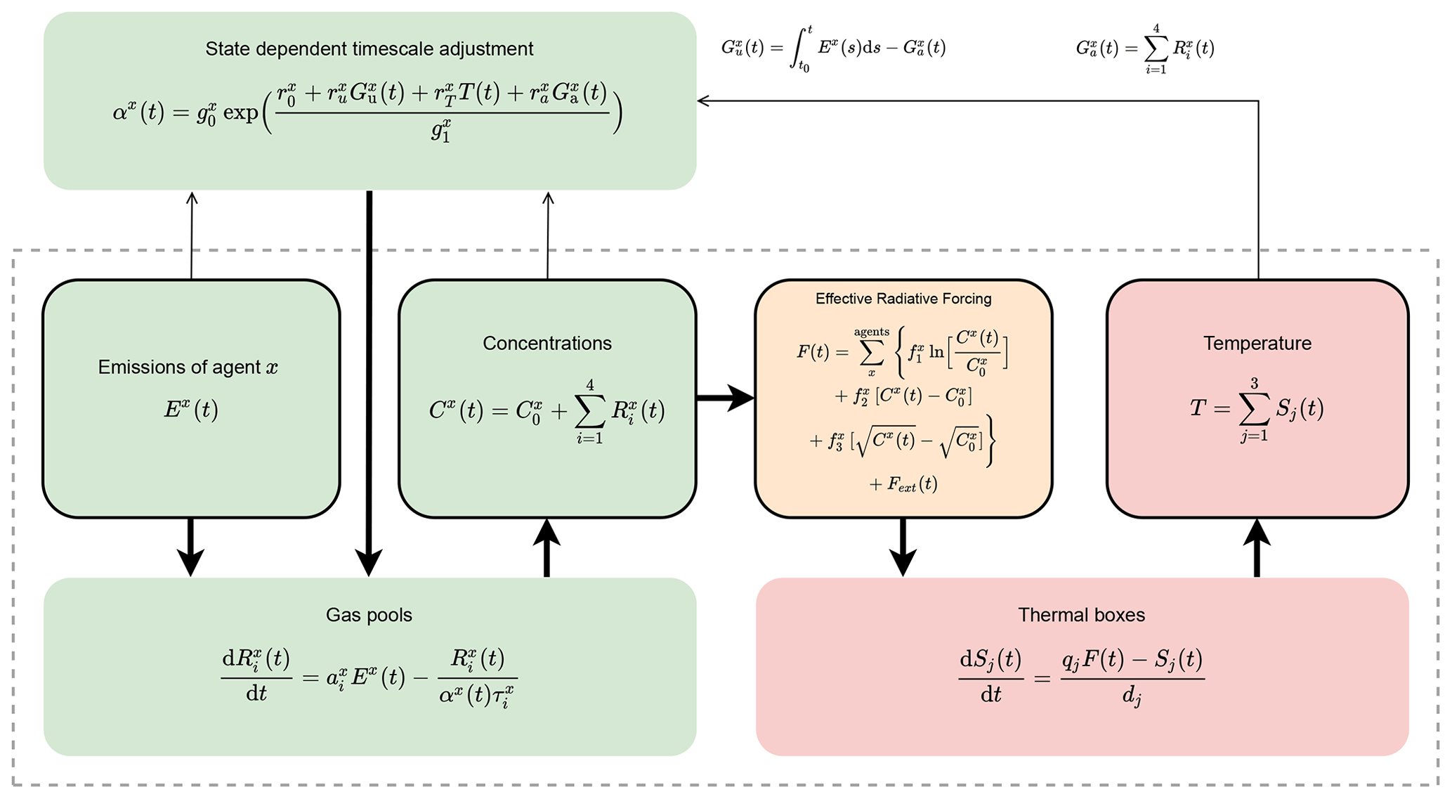
Figure 1 Schematic showing the full model structure and equations used. Terms without (t) are constants. Colouring splits the model into gas cycle, radiative forcing, and climate response components. The dashed grey line indicates the components identical to AR5-IR (Myhre et al., 2013). Table 1 provides brief descriptions of each named parameter in the figure. We note that under the default parameterization, for all gases except carbon dioxide, the index i and associated sums can be removed as these gases are modelled as having a single atmospheric decay timescale only. Equations are described in full in Sect. 2.1.

In FaIRv2.0.0 we propose a set of six equations that we demonstrate are sufficient to capture the global mean climate system response to GHG and aerosol emissions. These six equations are outlined in Fig. 1. In this text we explain the physical reasoning behind each equation and select a default parameter set based on simple tunings to historical observations and recent literature. We compare the default response of FaIRv2.0.0 to a publicly available version of the widely used SCM, MAGICC6 (Meinshausen et al., 2011a, b), for a range of socioeconomic pathways (Riahi et al., 2017, SSPs). Further, we show that these equations can be tuned to emulate key properties of a range of CMIP6 (Eyring et al., 2016) models. Finally, we constrain a large parameter ensemble inferred from more complex models and contemporary assessments with observations of the present-day warming level and rate to provide a set of observationally constrained probabilistic projections for the future climate following (Smith et al., 2018).

FaIRv2.0.0 is sufficiently simple as to be able to be used in undergraduate and high-school teaching of climate change and can illustrate some key properties of the climate system such as the warming impacts of different GHGs, the implications of uncertainty in ECS and transient climate response (TCR), or the importance of carbon cycle feedbacks. To allow students and other users unfamiliar with scientific programming languages (such as FaIRv2.0's native language, Python) access to the model, we also provide a version of FaIRv2.0.0 written in Excel. We hope that this may open exploration of the climate system to a large group of potential users who do not have the expertise to run presently available SCMs. The simplicity of FaIRv2.0.0 additionally means that although we provide code in a central, open-source repository, which we strongly recommend to be used for most cases, users are not forced to rely on this. In fact we expect it would be relatively quick to re-create in whatever language users are familiar with and in whatever format fits their intended usage.

Here we suggest that the major value of SCMs is in their ability to emulate more complex models, such as has been done in Meinshausen et al. (2011b); Tsutsui (2017, 2020), and their ability to efficiently integrate massive parameter ensembles for probabilistic climate projection as in Smith et al. (2018); Goodwin et al. (2019). While default parameters must be provided to enable unfamiliar users access to the model, the response arising from these parameters is a function of how they themselves have been selected, rather than one of the model equations themselves. So long as the underlying model equations are sufficiently flexible to emulate a wide range of climate system responses to the variables of interest (for instance the inferred range of responses within the CMIP ensemble) and have a basis in known physical processes, the SCM should be considered to be valid. Although understanding why the default response of SCMs differ is important, comparisons of solely the default response as a test of how “good” a model is are unhelpful; it is likely that any SCM could be re-tuned to better perform against whatever (single) metric is being used for evaluation, whether it is another SCM, a more complex model, or something else.

In this study we first outline the history and reasoning behind the model equations used in Sect. 2, including how we selected default parameters, stepping through the concentration response to emissions, the concentration–forcing relationships, and the thermal response to forcing. We then demonstrate how several key components of FaIRv2.0.0 – the carbon cycle, aerosol response, and thermal response to forcing – can be tuned to emulate a set of CMIP6 models in Sect. 3. Section 4 describes the use of FaIRv2.0.0 to constrain climate sensitivities and future surface temperature projections using a large ensemble following Smith et al. (2018). We then provide a discussion of previous comparisons of SCMs in Sect. 5 and suggest some ways in which FaIRv2.0.0 could be used in Sect. 6 before concluding.

2 FaIRv2.0.0 model framework

As with the previous iteration, FaIRv2.0.0 is a 0D model of globally averaged variables. It models the GHG emission → concentration → effective radiative forcing (ERF), aerosol emission → ERF, and ERF → temperature responses of the climate system. Here we present the equations behind these responses, separating out the model into the key components.

2.1 The gas cycle

FaIRv2.0.0 inherits the GHG gas cycle equations directly from the carbon cycle equations within FaIRv1.5 (Smith et al., 2018) and v1.0 (Millar et al., 2017). This carbon cycle adapts the four-timescale impulse response function for carbon dioxide in Joos et al. (2013) by introducing a state-dependent timescale adjustment factor, α. This factor scales the decay timescales of atmospheric carbon, allowing for the effective carbon sink from the atmosphere to change in strength. This allows FaIRv2.0.0 to represent non-linearities in the carbon cycle in a manner similar to Joos et al. (1996) or Hooss et al. (2001). In Millar et al. (2017), α was calculated through a parameterization of the 100-year integrated impulse response function (iIRF₁₀₀, the average airborne fraction over a period of 100 years). In Millar et al. (2017), the iIRF₁₀₀ was parameterized by a simple linear relationship with the quantity of carbon removed since initialization G_u, and the current temperature T:

$$\begin{array}{}\text{(1)}& {\text{iIRF}}_{\mathrm{100}}=r_{\mathrm{0}}+r_{\mathrm{u}}{G}_{\mathrm{u}}+r_{T}T,\end{array}$$

where r₀ is the initial (pre-industrial) iIRF₁₀₀ and r_u and r_T control how the iIRF₁₀₀ changes as the cumulative carbon uptake from the atmosphere and temperature change. This parameterization was informed by the behaviour of ESMs and remains consistent with the key feedbacks involved in the carbon cycle (Arora et al., 2020). However, in Millar et al. (2017), the root of an implicit non-linear equation had to be found to update α at each model time step. The solution of this equation is approximately exponential in iIRF₁₀₀ to a high degree of accuracy for a wide range of values, and thus in FaIRv2.0.0 α is calculated using the exponential form in Eq. (4). We parameterize this carbon cycle to enable it to simulate a wide range of GHGs, as discussed in Sect. 2.1.1. The equations for the carbon cycle and all other gas cycles are, in their most general form, as follows:

$$\begin{array}{}\text{(2)}& {\displaystyle \frac{\mathrm{d}{R}_i\left(t\right)}{\mathrm{d}t}}& {\displaystyle }=a_{i}E\left(t\right)-{\displaystyle \frac{R_i\left(t\right)}{\mathit{\alpha }\left(t\right){\mathit{\tau }}_i}},\text{(3)}& {\displaystyle }C\left(t\right)& {\displaystyle }=C_{\mathrm{0}}+\sum _{i=\mathrm{1}}^n{R}_i\left(t\right),\text{and}\text{(4)}& {\displaystyle }\mathit{\alpha }\left(t\right)& {\displaystyle }=g_{\mathrm{0}}\cdot \exp \left({\displaystyle \frac{r_{\mathrm{0}}+r_{\mathrm{u}}{G}_{\mathrm{u}}\left(t\right)+r_{T}T\left(t\right)+r_{\mathrm{a}}{G}_{\mathrm{a}}\left(t\right)}{g_{\mathrm{1}}}}\right);\end{array}$$

where

$$\begin{array}{ll}{\displaystyle }{G}_{\mathrm{a}}\left(t\right)& {\displaystyle }=\sum _{i=\mathrm{1}}^n{R}_i\left(t\right),\\ \text{(5)}& {\displaystyle }{G}_{\mathrm{u}}\left(t\right)& {\displaystyle }=\sum _{s=t_{\mathrm{0}}}^{t}E\left(s\right)-G_{\mathrm{a}}\left(t\right);\end{array}$$

and

$$\begin{array}{ll}{\displaystyle }{g}_{\mathrm{1}}& {\displaystyle }=\sum _{i=\mathrm{1}}^n{a}_i{\mathit{\tau }}_i\left[\mathrm{1}-\left(\mathrm{1}+\mathrm{100}/{\mathit{\tau }}_i\right){\text{e}}^{-\mathrm{100}/{\mathit{\tau }}_i}\right],\\ {\displaystyle }{g}_{\mathrm{0}}& {\displaystyle }=\exp \left(-{\displaystyle \frac{{\sum }_{i=\mathrm{1}}^n{a}_i{\mathit{\tau }}_i[\mathrm{1}-{\text{e}}^{-\mathrm{100}/{\mathit{\tau }}_i}]}{g_{\mathrm{1}}}}\right).\end{array}$$

Equations (2) and (3) describe a gas cycle with an atmospheric burden above the pre-industrial concentration, C₀, formed of n reservoirs: each reservoir corresponds to a different decay timescale from the atmosphere. These reservoirs do not correspond to any physical carbon stores, but qualitative analogies for them can be found in Millar et al. (2017). Each reservoir, R_i, has an uptake fraction a_i and decay timescale ατ_i. At each time step, the state-dependent adjustment, α, is computed and the reservoir concentrations are updated and aggregated to determine the new atmospheric burden. The new atmospheric concentration is then simply the sum of the burden and the pre-industrial concentration. Here we emphasize that although we have presented this equation set in its general form, with n reservoirs, in practice we set n=4 for the carbon cycle following Joos et al. (2013) and n=1 emissions for all other gases within FaIRv2.0.0. For the cases where n=1, Eqs. (2) and (3) can be simplified by dropping the index i entirely. α provides feedbacks to the gas lifetime(s) based on the current time step's levels of accumulated emissions (G_u), global temperature (T), and atmospheric burden (G_a). G_a is included to enable FaIRv2.0.0 to emulate the sensitivity of the CH₄ lifetime to its own atmospheric burden, as predicted by atmospheric chemistry and simulated in chemical transport models (CTMs) (Holmes et al., 2013; Prather et al., 2015). We also find that the emulation of the carbon cycle of a number of CMIP6 models over the 1 % CO₂ experiment is significantly improved if G_a is included in the iIRF₁₀₀ parameterization; see Sect. 3.2. In the default parameterization of FaIRv2.0.0, this state dependence is only active for carbon dioxide and methane; for all other gases, α is constant. g₀ and g₁ are constants that set the value and gradient of our analytic approximation for α equal to the numerical solution of the Millar et al. (2017) iIRF₁₀₀ parameterization at α=1 for the carbon cycle. An important point is that although we inherit the iIRF timescale of 100 years from Millar et al. (2017) and Joos et al. (2013), this timescale does not affect the behaviour of the model, only the quantitative values of the parameters. Hence, for a given emulation target (such as the C4MIP models in Sect. 3.2) the optimal model fit is independent of the length of this timescale, but the optimal parameter values are not. Maintaining this timescale at 100 years ensures that the r coefficients found here are comparable to the previous iterations of FaIR (Smith et al., 2018; Millar et al., 2017). In the following section, we discuss how we parameterize the gas cycle to enable FaIRv2.0.0 to simulate a wide range of GHGs using these same three equations. Qualitative analogies for each parameter are given in Table 1 to aid understanding.

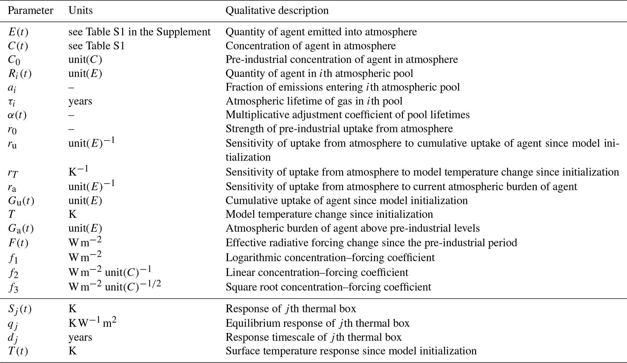
Table 1 Qualitative analogies for named parameters in FaIRv2.0.0.

Here we emphasize the advantage of using this common framework to simulate the response to all the different GHG and aerosol emissions: if a user is able to understand the FaIRv2.0.0 carbon cycle, then they understand how the model will respond to emissions of any other GHG or aerosol. This is because carbon dioxide is the most complex parameterization of the above equations: being the only species with more than one atmospheric decay timescale, and alongside methane it is one of only two species to make use of the state dependence through α within the default parameterization. This structural simplicity makes gaining familiarity with the model far easier than if several different gas cycle formulations were used for different GHGs.

2.1.1 Parameterizing the gas cycle for a wide range of GHGs

In this section, we consider how these equations can be parameterized to represent the gas cycles for many different GHGs. We also provide default parameterizations for each GHG, given in full in Table S2 in the Supplement.

Carbon dioxide

As discussed above in Sect. 2.1, FaIRv2.0.0 retains the state-dependent formulation (Millar et al., 2017) of the four-timescale impulse response model from Joos et al. (2013); hence, n=4. We retain the same state dependency as in Millar et al. (2017), and thus the r parameters are non-zero with the exception of r_a. The default a and τ coefficients are the multi-model mean from Joos et al. (2013). Default r_u and r_T parameters are taken as the mean of the parameter distributions inferred from CMIP6 models in Sect. 4.2.1. Following Jenkins et al. (2018), we tune the default r₀ parameter such that present-day (2018) cumulative CO₂ emissions match the RCMIP emission protocol (Nicholls et al., 2020a; Nicholls and Lewis, 2021) when historical concentrations (Meinshausen et al., 2017) are inverted back to emissions by Eqs. (2)–(4). Here we take the RCMIP protocol as one estimate of observed emissions, but it is important to note that using a different dataset such as the Global Carbon Project (Friedlingstein et al., 2019) would result in a different value. The pre-industrial concentration is fixed at 278 ppm.

Methane

We parameterize methane using a single atmospheric sink: n=1. Although several individual mechanisms have been identified for the removal of atmospheric methane – tropospheric OH, tropospheric Cl, stratospheric reactions, and soil uptake (Prather et al., 2012; Holmes et al., 2013) – these can be aggregated into a single effective atmospheric lifetime. Through r_T and r_a, we include the key lifetime feedback dependence on to its own atmospheric burden and tropospheric air temperature and water vapour mixing ratio (Holmes et al., 2013). We tune r_a to match the sensitivity of the methane lifetime to its own atmospheric burden at the present-day found by Holmes et al. (2013). r_T is tuned to match the sensitivity of the methane lifetime to tropospheric air temperature and water vapour at the present-day found by Holmes et al. (2013). Since both tropospheric air temperature and water vapour are closely related to surface air temperatures (they are often approximated by simple parameterizations of the surface air temperature, as in Holmes et al., 2013), including these two sensitivities through a single surface temperature feedback closely replicates lifetime behaviour if both are included separately. See Fig. S2 in the Supplement for the evolution of the methane lifetime within default FaIRv2.0.0 over history and a future RCP8.5 pathway (Riahi et al., 2011). τ is then set such that the mean emission rate since 2000 matches current estimates from the RCMIP protocol (Nicholls et al., 2020a; Nicholls and Lewis, 2021) when historical concentrations (Meinshausen et al., 2017) are inverted by FaIRv2.0.0, and r₀ is set such that α=1 at model initialization. The pre-industrial concentration is fixed at 720 ppb.

Nitrous oxide

Nitrous oxide is parameterized with a single atmospheric sink and no lifetime sensitivities: n=1 and $\mathit{\{}{r}_{\mathrm{u}},r_T,r_{\mathrm{a}}\mathit{\}}=\mathrm{0}$. Although there is evidence that nitrous oxide has a small sensitivity to its atmospheric burden (Prather et al., 2015), when included in FaIRv2.0.0 this made very little difference to nitrous oxide concentrations, even under high-emission scenarios. We therefore do not include this additional complexity. τ is tuned to match the cumulative RCMIP protocol emissions when historical concentrations are inverted by FaIRv2.0.0, and r₀ is set such that α=1 at model initialization. The pre-industrial concentration is fixed at 270 ppm.

Halogenated gases

All other GHGs are treated as having a single atmospheric lifetime and no feedbacks: n=1 and $\mathit{\{}{r}_{\mathrm{u}},r_T,r_{\mathrm{a}}\mathit{\}}=\mathrm{0}$. We take lifetime estimates from WMO (2018). Pre-industrial concentrations (if non-zero) are set to the 1750 CE value from Meinshausen et al. (2017). Inclusion of a temperature-dependent lifetime to represent changes to the Brewer–Dobson circulation (Butchart and Scaife, 2001), as in the MAGICC SCM (Meinshausen et al., 2011a), would be possible through a non-zero r_T parameter. We do not include a representation of this effect in our default parameterization due to its small impact on model output and increase in model complexity.

Aerosols

Aerosols have considerably shorter lifetimes than the timescales generally considered by SCMs (Kristiansen et al., 2016). In FaIRv2.0.0, as in previous iterations (Smith et al., 2018) and other SCMs (Meinshausen et al., 2011a), they are therefore converted directly from emissions to radiative forcing. In FaIRv2.0.0, this can be achieved by setting n=1, τ=1, and providing a unit conversion factor of 1 between emissions and “concentrations”.

2.1.2 Historical and SSP concentration trajectories

Here we compare the default parameterization gas cycle model in FaIRv2.0.0-alpha to a previous version, FaIRv1.5 (Smith et al., 2018), and to MAGICC7.1.0-beta (Meinshausen et al., 2020), highlighting any differences. All three models are run under the fully emission-driven “esm-allGHG” RCMIP protocol (Nicholls et al., 2020a; Nicholls and Lewis, 2021). FaIRv2.0.0 matches trajectories from both its previous iteration and the more comprehensive MAGICC closely for all GHGs. We note some discrepancies in the time series for halogenated gases between FaIRv2.0.0 and MAGICC, possibly due to the incorporation of a state-dependent OH abundance and representation of changes to the Brewer–Dobson circulation which modulate the lifetimes of these gases (Meinshausen et al., 2011a). We note that for these gases we could have matched historical concentrations closer by tuning the lifetimes to the RCMIP protocol data and historical concentration time series (Nicholls et al., 2020a; Meinshausen et al., 2017) but argue that taking the best-estimate lifetimes from WMO (2018) is defensible: it is more transparent and avoids source-dependent parameters (if a different emission dataset were used, the resulting tuned lifetimes would be different). The lower CO₂ concentration projections in FaIRv2.0.0 compared to FaIRv1.5 are due to weaker temperature and cumulative carbon uptake feedbacks (lower r_u and r_T) as inferred from the CMIP6 carbon cycle tunings performed in Sect. 3.2.

Specification of natural emissions

In FaIRv2.0.0 we have chosen to formulate the gas cycle equations in terms of a perturbation above the pre-industrial (natural equilibrium) concentration. By definition, this assumes a time-independent quantity of natural emissions for each gas (which can be derived from the pre-industrial concentration and lifetime of the gas). This differs from Meinshausen et al. (2011a) and Smith et al. (2018), who (when driving the respective models with emissions and with the exception of CO₂) require a quantity of natural emissions to be supplied in addition to any anthropogenic emissions by default (though the models can also be run in a fully emission-driven mode as in Fig. 2). Over the historical period, these emissions are chosen such that they “close the budget” between total anthropogenic emissions and observed concentrations (Meinshausen et al., 2011a; Smith et al., 2018). This procedure of balancing the budget over history is analogous to driving the model with concentrations up to the present day and then switching to driving the model with emissions afterwards. While this methodology has the advantage of ensuring the model simulates present-day concentrations that match observation exactly, it loses consistency between the way in which the model simulates the past and the future. If care is not taken when running these models, this loss of consistency could lead to discontinuities at the present day (when the model switches from concentration- to emission-driven). As present-day trends are crucial for the estimation of many policy and scientifically relevant quantities such as TCR, TCRE, and remaining carbon budgets (Leach et al., 2018; Tokarska et al., 2020; Jiménez-de-la Cuesta and Mauritsen, 2019), we have chosen to enforce a consistent model (i.e. emission-driven or concentration-driven) over the entire simulation period in FaIRv2.0.0. We note that replicating this budget closing procedure is possible in FaIRv2.0.0 by inverting observed concentrations to emissions and then joining these inverse emission time series to any future scenarios manually. In this study, FaIRv2.0.0 is run in emission-driven mode unless stated otherwise.

Figure 2 Comparison of historical and future concentration trajectories over a range of SSPs. Values for all GHGs are in parts per billion with the exception of CO₂, which is plotted in parts per million. Inset panels for CO₂, CH₄, and N₂O show the historic period.

2.2 Effective radiative forcing

FaIRv2.0.0 uses a simple formula to relate atmospheric gas concentrations to effective radiative forcing. This equation, Eq. (6), includes logarithmic, square-root, and linear terms, motivated by the concentration–forcing relationships in Myhre et al. (2013) of CO₂, CH₄ and N₂O, and all other well-mixed GHGs (WMGHGs), respectively. For most agents, the concentration–forcing (or for aerosols, emission–forcing) relationship can be reasonably approximated by one of these terms in isolation, however if there is substantial evidence the relationship deviates significantly from any one term, others are able to be included to provide a more accurate fit. F_ext is the sum of all exogenous forcings supplied. These may include natural forcing agents or forcing due to albedo changes.

$$\begin{array}{ll}\text{(6)}& {\displaystyle }F\left(t\right)=& {\displaystyle }\sum _x^{\text{forcing agents}}\mathit{\{}{f}_{\mathrm{1}}^x\cdot \text{ln}\left[{\displaystyle \frac{C^x\left(t\right)}{C_{\mathrm{0}}^x}}\right]+f_{\mathrm{2}}^x\cdot [C^x\left(t\right)-C_{\mathrm{0}}^x]{\displaystyle }& {\displaystyle }+f_{\mathrm{3}}^x\cdot \left[\sqrt{C^x\left(t\right)}-\sqrt{C_{\mathrm{0}}^x}\right]\mathit{\}}+F_{\text{ext}}\end{array}$$

2.2.1 Parameterizing the forcing equation

Carbon dioxide, nitrous oxide, and methane

We assume the forcing relationship for carbon dioxide is well approximated by the combination of a logarithmic and square-root term (Ramaswamy et al., 2001), $f_{\mathrm{2}}^{{\mathrm{CO}}_{\mathrm{2}}}=\mathrm{0}$; both the methane and nitrous oxide concentration–forcing relationships are approximated by a square-root term only: $f_{\mathrm{1},\mathrm{2}}^{{\mathrm{CH}}_{\mathrm{4}},{\mathrm{N}}_{\mathrm{2}}\mathrm{O}}=\mathrm{0}$. Although overlaps between the spectral bands of these gases mean more complex function forms including interaction terms represent our current best approximation to the observed relationship from spectral calculation (Etminan et al., 2016), inclusion of these interaction terms significantly increases the structural complexity of the model. These overlap terms are most significant for very high concentrations of these gases, and we find that the more simple relationships used here are sufficiently accurate within the context of the uncertainties associated with such high-concentration scenarios. We fit the non-zero f coefficients to the Oslo-line-by-line (OLBL) data from Etminan et al. (2016). Our resulting fits have a maximum absolute error of 0.115 W m⁻² when compared to the OLBL data, though this is for the most extreme high-concentration data point, and the associated relative error is 1.1 %. Figure S1 in the Supplement provides a complete comparison of how the fit relationships used here compare to the OLBL data and the simple formulae that include interaction terms in Etminan et al. (2016).

Halogenated GHGs

Following other simple models (Smith et al., 2018; Meinshausen et al., 2011a), we assume concentrations of halogenated gases are linearly related to their direct effective radiative forcing, $f_{\mathrm{1},\mathrm{3}}^x=\mathrm{0}$. The conversion coefficient for each gas is its radiative efficiency, which we take from WMO (2018).

Aerosol–radiation interaction

We follow Smith et al. (2020), parameterizing the ERF due to aerosol radiation interaction as a linear function of sulfate, organic carbon, and black carbon aerosol emissions:

$$\begin{array}{}\text{(7)}& \text{ERFari}=f_{\mathrm{2}}^{{\mathrm{SO}}_{\mathrm{2}}}{E}^{{\mathrm{SO}}_{\mathrm{2}}}+f_{\mathrm{2}}^{\mathrm{OC}}{E}^{\mathrm{OC}}+f_{\mathrm{2}}^{\mathrm{BC}}{E}^{\mathrm{BC}}.\end{array}$$

Default parameters are taken as the central estimate from the “constrained” ensemble described in Sect. 4.

Aerosol–cloud interaction

ERF due to aerosol–cloud interactions is parameterized following a modification of Smith et al. (2020), as a logarithmic function of sulfate aerosol emissions and a linear function of organic carbon and black carbon aerosol emissions:

$$\begin{array}{}\text{(8)}& \text{ERFaci}=f_{\mathrm{1}}^{\text{aci}}\ln \left(\mathrm{1}+{\displaystyle \frac{E^{{\mathrm{SO}}_{\mathrm{2}}}}{C_{\mathrm{0}}^{{\mathrm{SO}}_{\mathrm{2}}}}}\right)+f_{\mathrm{2}}^{\text{aci}}(E^{\mathrm{OC}}+E^{\mathrm{BC}}).\end{array}$$

Here $C_{\mathrm{0}}^{{\mathrm{SO}}_{\mathrm{2}}}$ effectively acts as a shape parameter for the logarithmic term. We fit this functional form to the ERFaci component in 10 CMIP6 models derived by the approximate partial radiative perturbation method (Zelinka et al., 2014) in Sect. 3.3. Default parameters are taken as the central estimate from the constrained ensemble described in Sect. 4.

Ozone

Ozone is parameterized following Thornhill et al. (2021), as a linear function of methane; nitrous oxide and ozone-depleting substances (ODSs) concentrations; and nitrate aerosol, carbon monoxide, and volatile organic compound emissions. This parameterization is tuned such that the overall ozone forcing time series reproduces Skeie et al. (2020). The contribution of individual ODSs to their total is based on their estimated equivalent effective stratospheric chlorine (Newman et al., 2007; Velders and Daniel, 2014; Smith et al., 2018), with fractional release factors from Engel et al. (2018).

Stratospheric water vapour

Stratospheric water vapour is assumed to be a linear function of methane concentrations (Smith et al., 2018) due to its small magnitude. The default coefficient is derived from the 5th Assessment Report forcing estimate (Myhre et al., 2013) and historical methane concentrations (Meinshausen et al., 2017): $\mathrm{4.37}\times {\mathrm{10}}^{-\mathrm{5}}$ $\mathrm{W}{\mathrm{m}}^{-\mathrm{2}}{\mathrm{ppb}}^{-\mathrm{1}}$.

Black carbon on snow

ERF due to light-absorbing particles on snow and ice remains a linear function of black carbon emissions (Smith et al., 2018). In AR5, the best estimate of its associated ERF was 0.04 W m⁻² (Myhre et al., 2013). However, this value is very uncertain, and the efficacy of black carbon on snow may at least double this value (Bond et al., 2013). We therefore calculate our default forcing efficiency by dividing an adopted value of −0.08 W m⁻² by the RCMIP protocol emission rate: 0.0116 $\mathrm{W}{\mathrm{m}}^{-\mathrm{2}}{\mathrm{MtBC}}^{-\mathrm{1}}$.

Contrails

Combined ERF due to contrails and contrail-induced cirrus is modelled as a linear function of aviation sector NO_x emissions. The default coefficient is calculated by dividing the best-estimate present-day contrail ERF (Lee et al., 2021) by the RCMIP protocol emission rate: 0.0164 $\mathrm{W}{\mathrm{m}}^{-\mathrm{2}}{{\mathrm{MtNO}}_x}^{-\mathrm{1}}$.

Albedo shift due to land use change

In this study we prescribe ERF due to land use change externally. However, it could be incorporated in a manner identical to FaIRv1.5 by supplying a time series of cumulative land use change CO₂ emissions and scaling linearly by a coefficient of −0.00114 $\mathrm{W}{\mathrm{m}}^{-\mathrm{2}}{\mathrm{GtC}}^{-\mathrm{1}}$ (Smith et al., 2018).

2.3 Default parameter metric values for comparison

Table S3 in the Supplement contains default parameter calculated values for the global warming potential (Lashof and Ahuja, 1990) of each emission type simulated in FaIRv2.0.0. These values are intended to aid comparison between FaIRv2.0.0 and other SCMs and do not represent any new analysis.

2.4 Temperature response

The final component of the model calculates the surface temperature response to the changes in ERF. A common representation of this physical process is the energy balance model outlined by Geoffroy et al. (2013). Here we consider the three-box energy balance model, including the ocean heat uptake efficacy factor introduced by Held et al. (2010). Recent literature has suggested that a two-box energy balance model is insufficient to capture the full range of behaviour observed in CMIP6 models (Tsutsui, 2020, 2017; Cummins et al., 2020). The three-box model can be written in state space form as follows:

$$\begin{array}{ll}\text{(9)}& {\displaystyle }\dot{\mathit{X}}\left(t\right)& {\displaystyle }=\mathbf{A}\mathit{X}\left(t\right)+\mathit{b}F\left(t\right),{\displaystyle }\text{where}\mathit{X}\left(t\right)& {\displaystyle }={\left(\begin{array}{ccc}{T}_{\mathrm{1}}\left(t\right)& T_{\mathrm{2}}\left(t\right)& T_{\mathrm{3}}\left(t\right)\end{array}\right)}^T,\\ {\displaystyle }\mathbf{A}& {\displaystyle }=,\\ {\displaystyle }\text{and}\mathit{b}& {\displaystyle }={\left(\begin{array}{ccc}\mathrm{1}/C_{\mathrm{1}}& \mathrm{0}& \mathrm{0}\end{array}\right)}^T.\end{array}$$

Here, each box i has a temperature T_i and heat capacity C_i. F is the prescribed radiative forcing. Heat exchange coefficients κ represent the strength of thermal coupling between boxes i and i−1. λ is the so-called climate feedback parameter. ϵ is the efficacy factor that enables the energy balance model to account for the variations in λ during periods of transient warming observed in general circulation models (GCMs). T₁ represents the surface temperature change relative to a pre-industrial climate. For many users of SCMs, the key variable of interest is T₁, i.e. the surface temperature response. To allow parameters of this energy balance model to be fit to finite-length CMIP6 experiments with any degree of certainty, Cummins et al. (2020) also take advantage of the following relationship with the top of atmosphere flux, N(t):

$$\begin{array}{}\text{(10)}& N\left(t\right)=F\left(t\right)-\mathit{\lambda }{T}_{\mathrm{1}}\left(t\right)+(\mathrm{1}-\mathit{ϵ}){\mathit{\kappa }}_{\mathrm{3}}\left[T_{\mathrm{2}}\right(t)-T_{\mathrm{3}}(t\left)\right].\end{array}$$

However, calculating the surface temperature response to radiative forcing within the energy balance model can be simplified by diagonalizing Eq. (9), resulting in an impulse response in T₁ (henceforth referred to as T), giving the thermal response form in Millar et al. (2017) (Tsutsui, 2017):

$$\begin{array}{}\text{(11)}& {\displaystyle \frac{\mathrm{d}{S}_j\left(t\right)}{\mathrm{d}t}}& {\displaystyle }={\displaystyle \frac{q_{j}F\left(t\right)-S_j\left(t\right)}{d_j}},\text{(12)}& {\displaystyle }\text{and}T\left(t\right)& {\displaystyle }=\sum _{j=\mathrm{1}}^{\mathrm{3}}{S}_j\left(t\right).\end{array}$$

We can relate the energy balance model matrix representation to the impulse response parameters as follows. If we let Φ be the matrix that diagonalizes A such that ${\mathbf{\Phi }}^{-\mathrm{1}}\mathbf{A}\mathbf{\Phi }=\mathbf{D}$, where D is a diagonal matrix with the eigenvalues of A on the diagonals, then the response timescales are $d_i=-\mathrm{1}/D_{ii}$ (Geoffroy et al., 2013). The response coefficients are $q_i=d_i{\mathrm{\Phi }}_{i,\mathrm{0}}^{-\mathrm{1}}{\mathrm{\Phi }}_{\mathrm{0},i}/C_{\mathrm{1}}$. In FaIRv2.0.0, we use this three-timescale impulse response form due to its simplicity and flexibility. Two common measures of the climate sensitivity, the equilibrium climate sensitivity (ECS) and transient climate response (TCR) (Collins et al., 2013) are easily expressed in terms of the impulse response parameters:

$$\begin{array}{}\text{(13)}& {\displaystyle }\text{ECS}& {\displaystyle }=F_{\mathrm{2}\times {\mathrm{CO}}_{\mathrm{2}}}\cdot \sum _{j=\mathrm{1}}^{\mathrm{3}}{q}_j,\text{(14)}& {\displaystyle }\text{TCR}& {\displaystyle }=F_{\mathrm{2}\times {\mathrm{CO}}_{\mathrm{2}}}\cdot \sum _{j=\mathrm{1}}^{\mathrm{3}}\left\{q_j\left(\mathrm{1}-{\displaystyle \frac{d_j}{\mathrm{70}}}\left[\mathrm{1}-e^{-\frac{\mathrm{70}}{d_j}}\right]\right)\right\}.\end{array}$$

The default thermal response parameters in FaIRv2.0.0 are derived as follows: d₁=0.903, d₂=7.92, d₃=355, and q₁=0.180 are taken as their central value within the constrained ensemble in Sect. 4.3, which do not differ significantly from the CMIP6 inferred distribution described in Sect. 4.2.3. q₂=0.297 and q₃=0.386 are then set by Eqs. (13) and (14) such that the default parameter set response has climate sensitivities (ECS and TCR) equal to the central values of the constrained ensemble described in Sect. 4: ECS=3.24 K and TCR=1.79 K.

3 Emulating complex climate models

In this section we demonstrate the ability of FaIRv2.0.0 to emulate the more complex models from CMIP6 (Eyring et al., 2016) in a limited set of experiments. Due to constraints on data availability, we have focussed on tuning the key components of the model: the carbon cycle, the thermal response, and the aerosol ERF relationships. We use the abrupt-4xCO2 and 1pctCO2 CMIP6 experiments to tune the carbon cycle and thermal response. The highly idealized nature of these experiments means that parameters arising from these tunings will not necessarily be able to emulate complex model response to more realistic scenarios due to processes that FaIRv2.0.0 cannot represent. In the near future we hope to be able to tune to the historical and SSP CMIP6 experiments in order to validate the tunings given here.

3.1 Tuning the thermal response

We follow the statistically rigorous methodology of Cummins et al. (2020) to tune thermal response parameters to 28 CMIP6 models. This involves fitting parameters to the energy balance model outlined in Eq. (9) by recursively computing the likelihood via a Kalman filter; the optimal parameters are those that maximize the computed likelihood. We then transform the optimal energy balance parameters into the impulse response form used in FaIRv2.0.0. We obtain model data from the “abrupt-4xCO2”, “1pctCO2” and “piControl” experiments for the top-of-energy imbalance and surface temperature response from ESGF (Cinquini et al., 2014). These data are normalized as described in Nicholls et al. (2021). To reduce internal variability in the input time series used to fit parameters, we average over all available ensemble members for each model. The number of ensemble members per model is stated in Table S4 in the Supplement. The Cummins et al. (2020) methodology uses surface temperatures and top-of-atmosphere energy imbalances (as related by Eq. 10) from the abrupt-4xCO2 experiment to return all the parameters of the energy balance model, plus the radiative forcing arising from the quadrupling of carbon dioxide concentrations. While this would fully specify both the thermal response and the concentration–forcing relationship if concentration–forcing was a pure logarithmic relationship, several models display significant deviations from a pure logarithmic concentration–forcing relationship (Tsutsui, 2020, 2017). We account for this within the FaIRv2.0.0 framework by assuming that the concentration–forcing relationship can be reasonably approximated by the sum of a logarithmic and square-root term. Best-estimate $f_{\mathrm{1}}^{{\mathrm{CO}}_{\mathrm{2}}}$ and $f_{\mathrm{3}}^{{\mathrm{CO}}_{\mathrm{2}}}$ parameters are found by first deriving the TCR of each model using the 1pctCO2 experiment. We can use the tuned impulse response parameters and TCR to then calculate the forcing at a doubling of carbon dioxide using the relationship in Eq. (14). The forcings at carbon dioxide doubling and quadrupling uniquely specify $f_{\mathrm{1}}^{{\mathrm{CO}}_{\mathrm{2}}}$ and $f_{\mathrm{3}}^{{\mathrm{CO}}_{\mathrm{2}}}$ values for use in FaIRv2.0.0. The best-estimate impulse response and f parameters, climate sensitivities, and forcings at carbon dioxide doubling and quadrupling are given in Table 2. Corresponding energy balance model parameters are given in Table S5. Figure 3 shows the emulated and original responses to the abrupt-4xCO2 and 1pctCO2 experiments for each model.

Table 2 Tuned CMIP6 thermal response parameters.

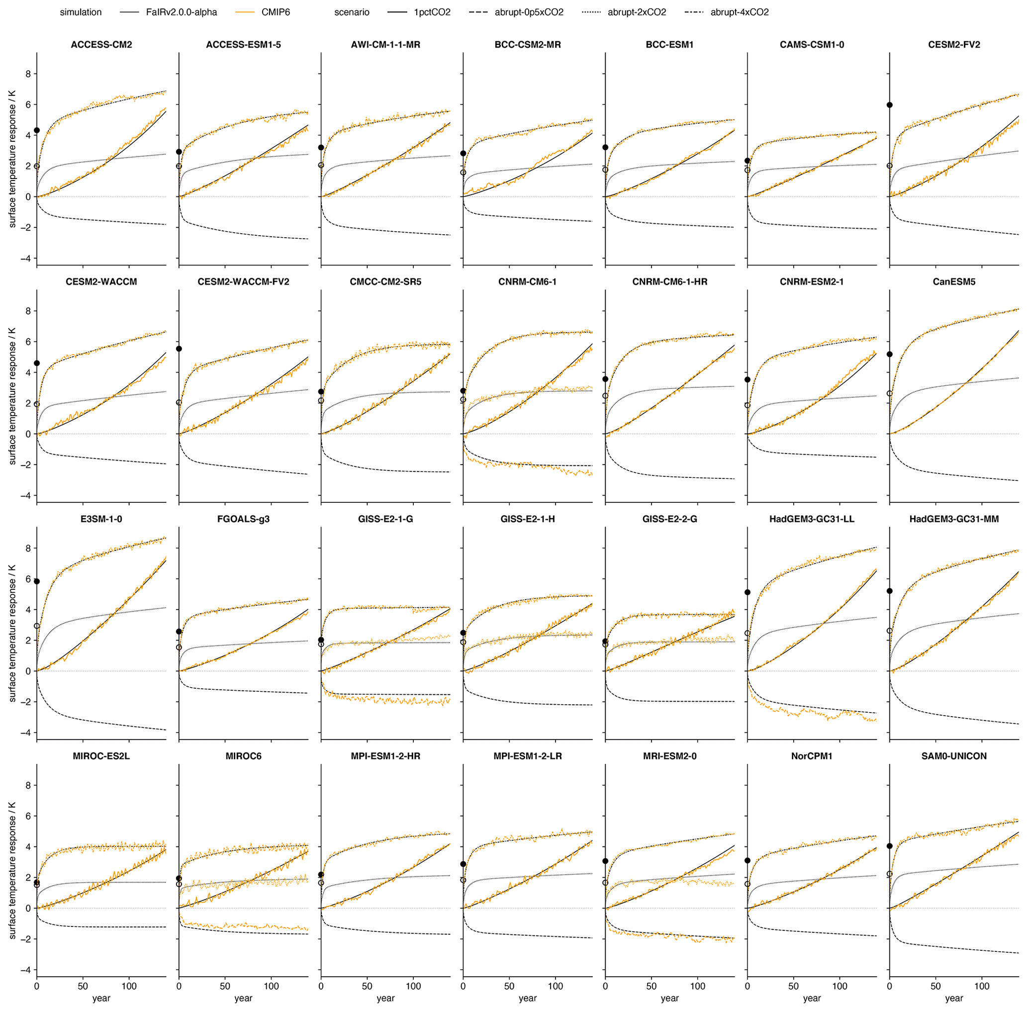
Figure 3 FaIRv2.0.0 emulation of CMIP6 model response to the abrupt-4xCO2, abrupt-2xCO2, abrupt-0p5xCO2, and 1pctCO2 experiments. The black line shows FaIRv2.0.0-alpha emulation, and the orange line shows CMIP6 model data where available. Emulation parameters were fit using the abrupt-4xCO2 and 1pctCO2 experiments so the abrupt-2xCO2 and abrupt-0p5xCO2 simulations can be considered as verification experiments for the models where the data for these experiments is available. Filled and unfilled dots over the y axis indicate the assessed model ECS and TCR, respectively (see Table 2).

3.2 Tuning the carbon cycle response

We tune the carbon cycle using CMIP6 data from the C4MIP (Jones et al., 2016) fully coupled and biogeochemically coupled 1pctCO2 runs (Arora et al., 2020). Since constraining the response coefficients a_i and timescales τ_i requires pulse emission experiments such as those carried out by Joos et al. (2013), here we only fit the r feedback parameters and keep the response coefficients, a, and timescales, τ, equal to the multi-model mean from Joos et al. (2013). The inclusion of both the fully coupled and biogeochemically coupled runs in the procedure allows us to constrain r_u, r_a, and r_T independently. We use Eqs. (2) and (3) to diagnose the values of α required to reproduce the C4MIP emissions from the corresponding concentrations within the FaIRv2.0.0 carbon cycle impulse response framework. We then use Eq. (4) to convert α into iIRF₁₀₀ time series. Finally, we use an ordinary least-squares estimator to calculate r parameters by regressing the C4MIP cumulative uptake, temperature, and atmospheric burden time series against the diagnosed iIRF₁₀₀ time series. r₀ is taken as the intercept of the estimator. We include the atmospheric burden as a predictor (and hence obtain non-zero r_a values) due to a significant reduction in regression residual for several models when included. We find that all the C4MIP models display an exceptionally high, rapidly decreasing initial airborne fraction. In terms of the FaIRv2.0.0 equations, this corresponds to an α value that decreases initially before reaching a minimum, representing a carbon sink that initially increases in strength when concentrations start to rise before decreasing as the concentrations and temperatures rise further. FaIRv2.0.0 is unable to fully capture this initial adjustment, and as such in our tunings we prioritize emulating the long-term behaviour and carry out the regression from year 60 onwards. It would be possible to better capture the initial adjustment by including additional terms in Eq. (4), but since it remains to be seen whether this behaviour is apparent in scenarios where concentrations do not rise suddenly and rapidly from a pre-industrial level as is the case in the 1pctCO₂ experiment (such as a historical emission scenario), we do not do so here. Tuned parameters are given in Table 3, with Fig. 4 showing diagnosed C4MIP emissions and the FaIRv2.0.0-alpha emulation. We note that these tunings suggest that the pre-industrial sink strength (which is encapsulated by r₀) in 7 out of 11 models is higher than the historically observed best estimate found here (Sect. 2.1.1) and in a previous study (Jenkins et al., 2018).

Table 3 Tuned CMIP6 carbon cycle parameters.

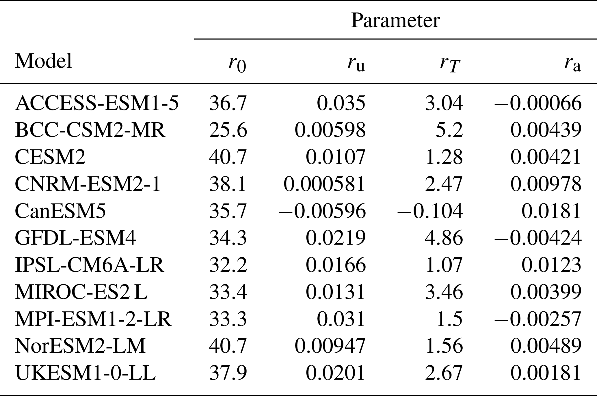
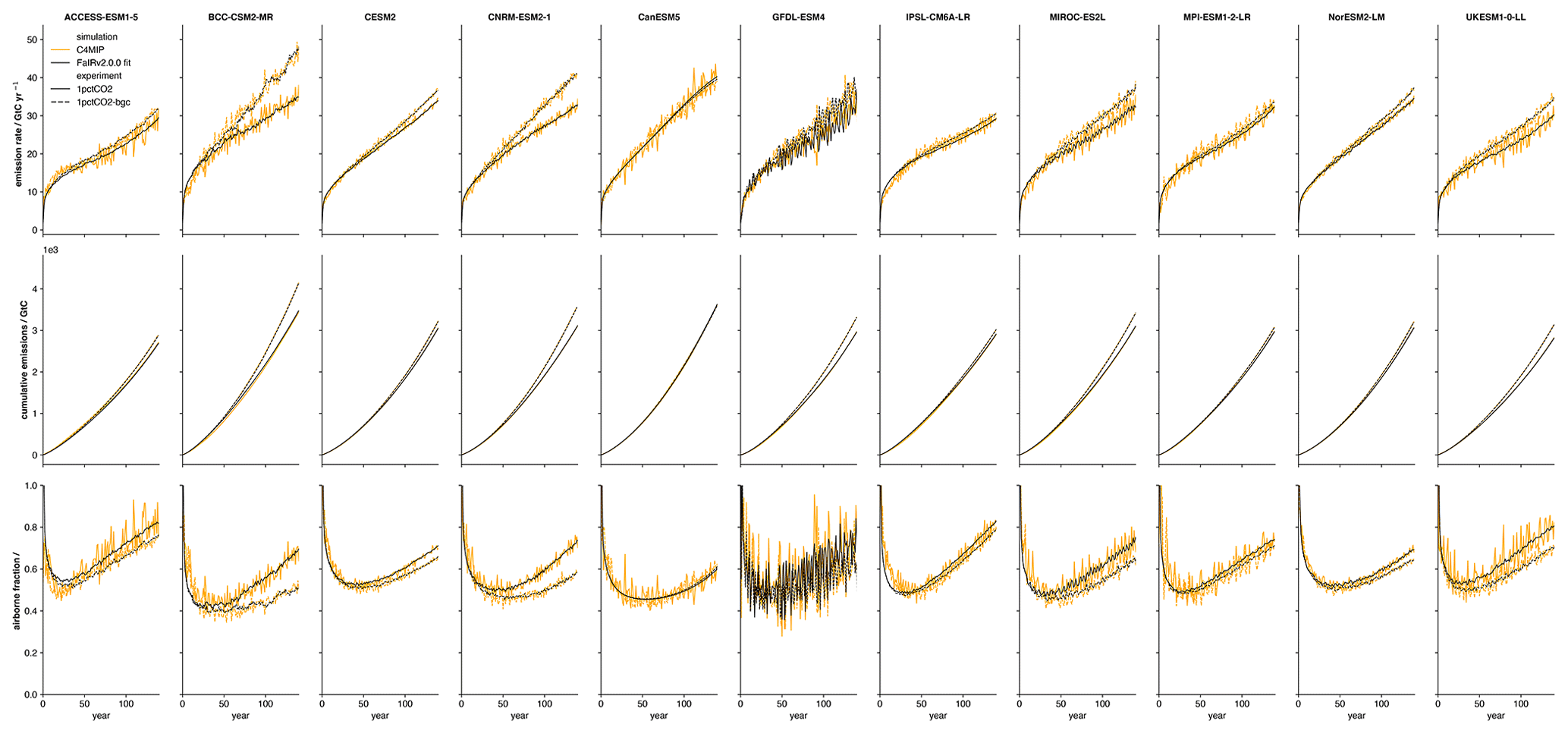
Figure 4 FaIRv2.0.0 emulation of CMIP6 model carbon cycle response to the C4MIP 1pctCO2 experiments. The black line shows FaIRv2.0.0-alpha emulation, and the orange line shows C4MIP model data. The top row shows diagnosed emission rates, the middle row shows cumulative emissions, and the bottom row shows airborne fraction. The solid line indicates the fully coupled C4MIP runs, while the dashed lines show biogeochemically coupled runs (emulated in FaIRv2.0.0-alpha by setting r_T=0).

3.3 Tuning aerosol ERF

Aerosol forcing relationships are tuned to ERF data from 10 CMIP6 models and emission data from the RCMIP protocol (Nicholls et al., 2020a; Nicholls and Lewis, 2021) following Smith et al. (2020). For each CMIP6 model, aerosol–radiation and aerosol–cloud interaction components of the ERF are calculated by the approximate partial radiative perturbation (APRP) method. For additional details on the exact procedure, see Smith et al. (2020) and Zelinka et al. (2014). For each model, we fit the f coefficients in Eq. (7) to the ERFari component using an ordinary least-squares estimator. The resulting coefficients are almost identical to those from Smith et al. (2020), with differences arising only due to the emission data used. We then fit the f coefficients and $C_{\mathrm{0}}^{{\mathrm{SO}}_{\mathrm{2}}}$ in Eq. (8) to the ERFaci component by minimizing the residual sum of squares using a simplex algorithm (Nelder and Mead, 1965). The tuned parameters are given in Table 4. Figure 5, following Fig. 2 of Smith et al. (2020), shows the parameterized fits compared to the APRP-derived model ERF components.

Table 4 Tuned CMIP6 aerosol forcing parameters.

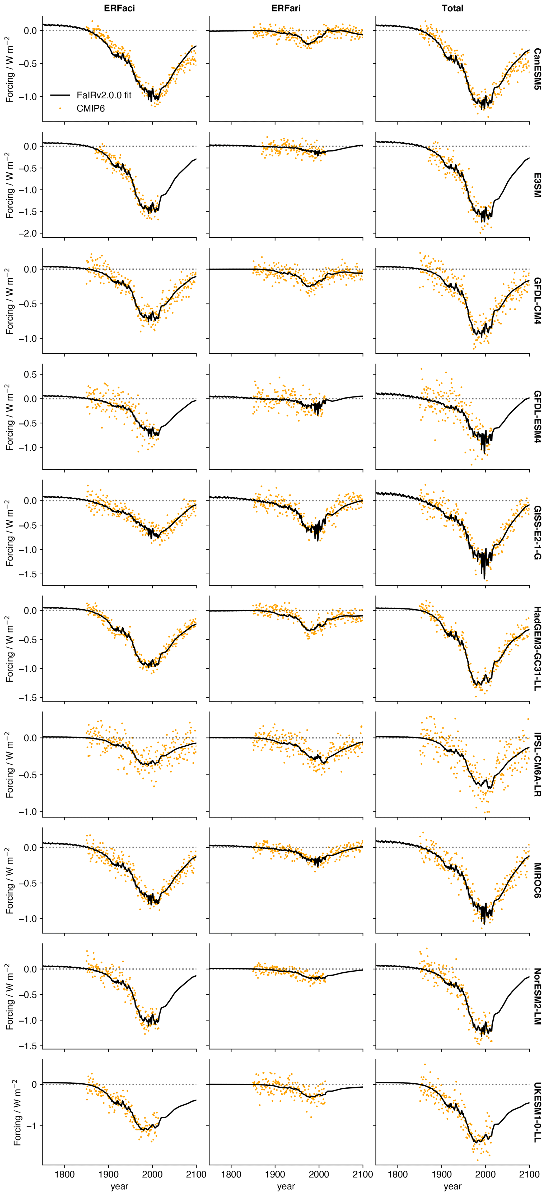
Figure 5 FaIRv2.0.0 emulation of CMIP6 model aerosol forcing. The black line shows FaIRv2.0.0-alpha emulation, and the orange dots show CMIP6 model data. All series displayed are relative to zero effective radiative forcing in 1850.

4 Constraining probabilistic parameter ensembles

The computational efficiency of SCMs makes them an ideal tool for carrying out large ensemble simulations from which probabilistic projections can be derived. Smith et al. (2018) carried out such a large ensemble and produced projections based on constraining the ensemble members to fall within the 5 %–95 % uncertainty range in observed warming to date from the Cowtan and Way dataset (Cowtan and Way, 2014). Here we replicate this procedure with the new model but using a new constraint methodology and updated prior parameters distributions.

4.1 The current level and rate of warming

We determine the current level and rate of warming following the Global Warming Index methodology (Haustein et al., 2017). This takes into account multiple sources of uncertainty: observational, forcing, Earth system response (through parameter variation in an identical climate response model to the one used in FaIRv2.0.0), and internal variability. With this methodology, we obtain an estimate of the distribution of the current (2010–2019) level and rate of the anthropogenic contribution to global warming (the anthropogenic warming index distribution). A key choice within this estimate is the observational data product used. There are six widely used products available (Lenssen et al., 2019; Cowtan and Way, 2014; Vose et al., 2012; Morice et al., 2012, 2020; Rohde et al., 2013). Here we average over the distributions implied by each product to obtain our final distribution used to constrain our FaIRv2.0.0 ensemble. This choice clearly projects significantly onto our results, so we provide results for each dataset in turn in Sect. 4.3.5 to demonstrate the sensitivity of our analysis to the choice of dataset. For full details of this calculation, see the Supplement.

4.1.1 Definition of global mean temperature

Recent studies (Richardson et al., 2016, 2018) have shown that the definition of globally averaged surface temperature used is important when comparing observations to climate model output, and is relevant when exploring policy-relevant quantities such as the carbon budget (Tokarska et al., 2019). Discrepancies arise since observations blend air temperatures over land and sea ice with water temperature over ocean and do not have full global coverage (they are blended–masked), while climate model surface temperature output is globally complete and always measured as the air temperature 2 m above the surface of the Earth. It has been shown both historically and over future climate scenarios (Richardson et al., 2018) that the blended–masked temperature definition (GMST) may be cooler than the globally complete 2 m air temperature definition (GSAT). In our Global Warming Index calculation (Sect. 4.1), we combine six temperature observation datasets (Lenssen et al., 2019; Cowtan and Way, 2014; Vose et al., 2012; Morice et al., 2012; Rohde et al., 2013; Morice et al., 2020); this implies that our constrained ensemble will broadly measure surface temperatures using the GMST definition. This may lead to slightly lower model estimates of surface temperature than if we used the GSAT definition. We can estimate the difference between our definition of GMST and GSAT by regressing the six-dataset mean used here against GSAT from ERA5 (Hersbach et al., 2020). A least-squares estimator (confidence calculated using a block-bootstrap; Wilks, 1997) suggests that our GMST definition is 4.6 % [0.4 %, 10.8 %] smaller than GSAT².

4.2 Sampled prior distributions

4.2.1 Carbon cycle parameters

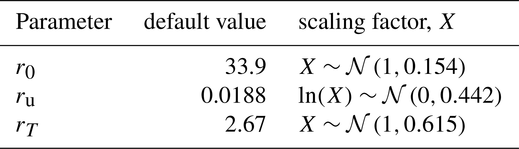
While including the atmospheric burden is necessary to emulate the carbon cycle behaviour of individual C4MIP models well, parameterizing the iIRF₁₀₀ as a linear function of just cumulative carbon uptake and temperature is sufficient to capture the spread of the model ensemble. Correlations between parameters also complicate sampling from the inferred parameter distributions derived from Table 3. We therefore repeat the parameter tuning procedure described in Sect. 3.2 but exclude the atmospheric burden as a predictor for the C4MIP iIRF₁₀₀ time series. The resulting r₀, r_u, and r_T parameter samples are uncorrelated. We sample these parameters by applying scaling factors inferred from the CMIP6 tunings to the default parameter values (for r_u and r_T this is equivalent to sampling directly from the distribution inferred from the CMIP6 tunings). The underlying uncorrelated scaling factor distributions are given in Table 5.

Table 5 Carbon cycle parameter sampling.

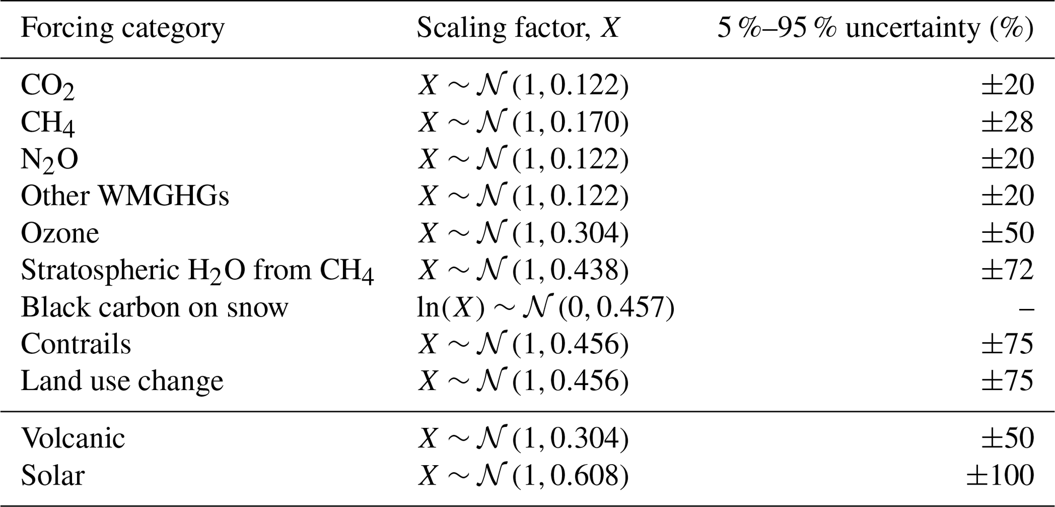
4.2.2 Forcing parameters

Uncertainty in effective radiative forcing is included by grouping individual forcing agents into broader forcing classes (IPCC et al., 2013) and applying a randomly sampled scaling factor to all the f parameters within each class (with the exception of aerosol forcings, which we discuss immediately below). Scaling factors between forcing classes are uncorrelated. The scaling factor distributions used for each forcing class are given in Table 6. Uncertainty in aerosol forcing is included as follows. ERFari f coefficients (Eq. 7) are first drawn from a multivariate normal distribution inferred from the CMIP6 tuned parameters in Table 4. We then apply a quantile map to scale the resulting coefficients such that the 1850 to 2005–2015 mean ERFari distribution matches the process based assessment in Bellouin et al. (2020). For ERFaci, $f_{\mathrm{2}}^{\text{aci}}$ coefficients (Eq. 8) are drawn from a normal distribution inferred from the CMIP6 tuned parameters in Table 4. $f_{\mathrm{1}}^{\text{aci}}$ and $C_{\mathrm{0}}^{{\mathrm{SO}}_{\mathrm{2}}}$ coefficients are drawn from a multivariate log-normal distribution; this ensures we sample the full range of ERFaci shapes provided by CMIP6 models. As with the ERFari coefficients, we then apply a quantile map to scale these coefficients such that the sampled 1850 to 2005–2015 mean ERFaci distribution matches Bellouin et al. (2020).

Table 6 ERF parameter sampling.

4.2.3 Thermal response parameters

Uncertainty in thermal response is incorporated by sampling response parameters directly from distributions inferred from the CMIP6 tunings in Sect. 2, taking correlations between parameters into account. Referring to parameters as in Eqs. (11)–(14), we draw parameters from the following distributions. d₁, d₂, and q₁ are highly correlated, and we therefore sample ln(d₁), ln(d₂), and q₁ from a multivariate normal distribution with covariances and means taken from the values in Sect. 2. d₃ is not strongly correlated with any other parameter, and so we sample ln(d₃) from a normal distribution. We then independently sample the TCR and the $\text{TCR}/\text{ECS}$ ratio, i.e. the realized warming fraction (RWF), as it has been shown that the TCR and RWF are much more weakly correlated than any other combination of ECS, TCR, and RWF (Millar et al., 2015). We draw TCR samples from a normal distribution, $\text{TCR}\sim \mathcal{N}\left(\mathrm{2},\mathrm{0.608}\right)$, truncating the distribution at a distance of ±3σ from the central value of 2. We draw RWF samples from a normal distribution $\text{RWF}\sim \mathcal{N}\left(\mathrm{0.55},\mathrm{0.15}\right)$, again truncating at ±3σ. The 90 % credible interval of the sampled TCR and RWF distributions closely (but not exactly) match the ranges inferred from the parameters in Table 2. Using Eqs. (13) and (14), we then calculate q₂ and q₃. We reject any samples in which any of the q parameters are unphysical (negative). The quantiles of the prior ECS and TCR distributions used are given in Table 7.

4.3 The constrained ensemble

Taking historical and future SSP (Riahi et al., 2017) emissions from the RCMIP protocol (Nicholls et al., 2020a; Nicholls and Lewis, 2021) and land use change, volcanic, and solar forcing from the SSP effective radiative forcing time series (Smith, 2020), we run a 1 000 000 member emission-driven ensemble (“full”), sampling uncertainty in the carbon cycle, effective radiative forcing, and thermal response as described in Sects. 4.2.1, 4.2.2, and 4.2.3. This full ensemble is then constrained by setting the selection probability of each member equal to the likelihood of its simulated present-day level and rate of anthropogenic warming within the anthropogenic warming index distribution. These likelihoods are calculated using a binning procedure at a resolution of 0.01 K (level) and 0.001 K yr⁻¹ (rate). Finally, we subsample the full ensemble based on these selection probabilities to generate the constrained ensemble. This procedure retains 9.6 % of the full ensemble. Table 7 outlines the results of this analysis in terms of the quantiles of key metrics: the model climate sensitivity and present-day radiative forcing.

Table 7 Constrained ensemble results for climate sensitivities and current ERF. ERF in 2019 is based on following an SSP2-4.5 pathway from 2014 onwards.

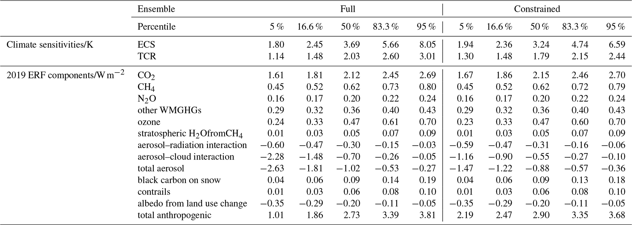
4.3.1 Current effective radiative forcing

The constraint applied only significantly affects the estimated ranges of ERFaci, total aerosol, and anthropogenic forcings in 2019 (based on an SSP2-45 pathway following 2014). ERFaci is constrained from −0.70 [−2.28, −0.05] to −0.55 [−1.16, −0.10], total aerosol forcing is constrained from −1.02 [−2.63, −0.27] to −0.88 [−1.47, −0.36], and total anthropogenic forcing is constrained from 2.73 [1.01, 3.81] to 2.90 [2.19, 3.68]. These results are consistent with a recent study that used similar methods but concentrated on aerosol forcing and used a constraint based on observed warming and Earth energy uptake (Smith et al., 2020). Other forcing categories are not affected by the constraint due to their relatively small magnitude and/or prior uncertainty.

4.3.2 Climate sensitivities

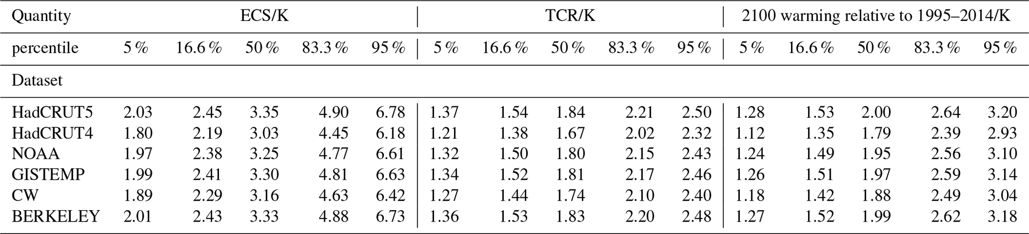
We find that the TCR is constrained from 2.03 [1.14, 3.01] to 1.79 [1.30, 2.44] and that the ECS is constrained from 3.69 [1.80, 8.05] to 3.24 [1.94, 6.59]. These results are consistent with several recent studies that have used emergent constraint techniques (Fig. 6, Nijsse et al., 2020; Jiménez-de-la Cuesta and Mauritsen, 2019; Tokarska et al., 2020; Brunner et al., 2020; Ribes et al., 2021) or drew on multiple lines of evidence (Sherwood et al., 2020); our constrained likely range of TCR exactly matches Sherwood et al. (2020) to two significant places. The largest discrepancies with these studies occur at the upper tails of the constrained ECS distribution; the constraint applied here is unable to rule out higher values of the ECS that some of these other studies have done. The constrained RWF distribution does not differ significantly from the prior distribution of 0.55 [0.3, 0.8].

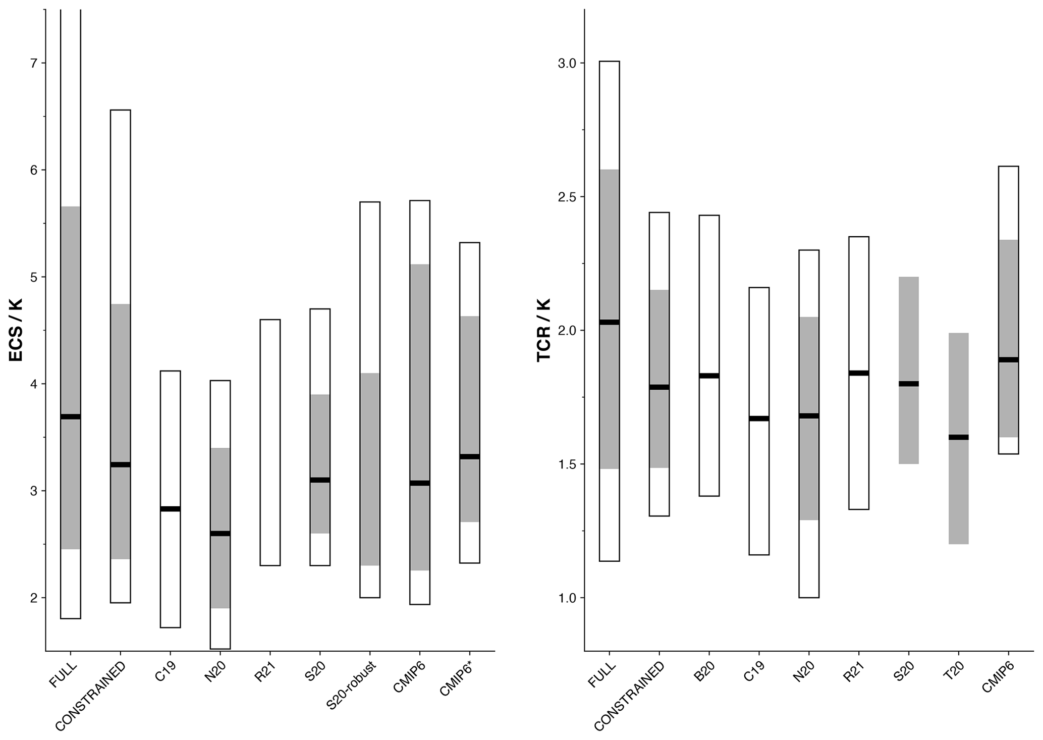
Figure 6 Climate sensitivities of our full and constrained ensembles in the context of other studies. The black line indicates median values, the grey shading shows the likely range, and unfilled bars show the 5 %–95 % range. Studies included are as follows: Brunner et al. (2020, B20), Jiménez-de-la Cuesta and Mauritsen (2019, C19), Nijsse et al. (2020, N20), Ribes et al. (2021, R21), Sherwood et al. (2020, S20), Tokarska et al. (2020, T20). CMIP6 indicates climate sensitivities derived from the energy balance model fits calculated in Sect. 3.1 (including ocean heat uptake efficacy); CMIP6* indicates climate sensitivities derived using the Gregory method (Gregory et al., 2004) over the first 150 years of the abrupt-4xCO2 experiment.

4.3.3 Correlations between climate sensitivities and ERF

There are significant correlations between key variables in the constrained ensemble, consistent with previous studies (Smith et al., 2018; Millar et al., 2015; Sanderson, 2020; Forest et al., 2002; Marvel et al., 2016). These are shown in the contour plots in Fig. 7.

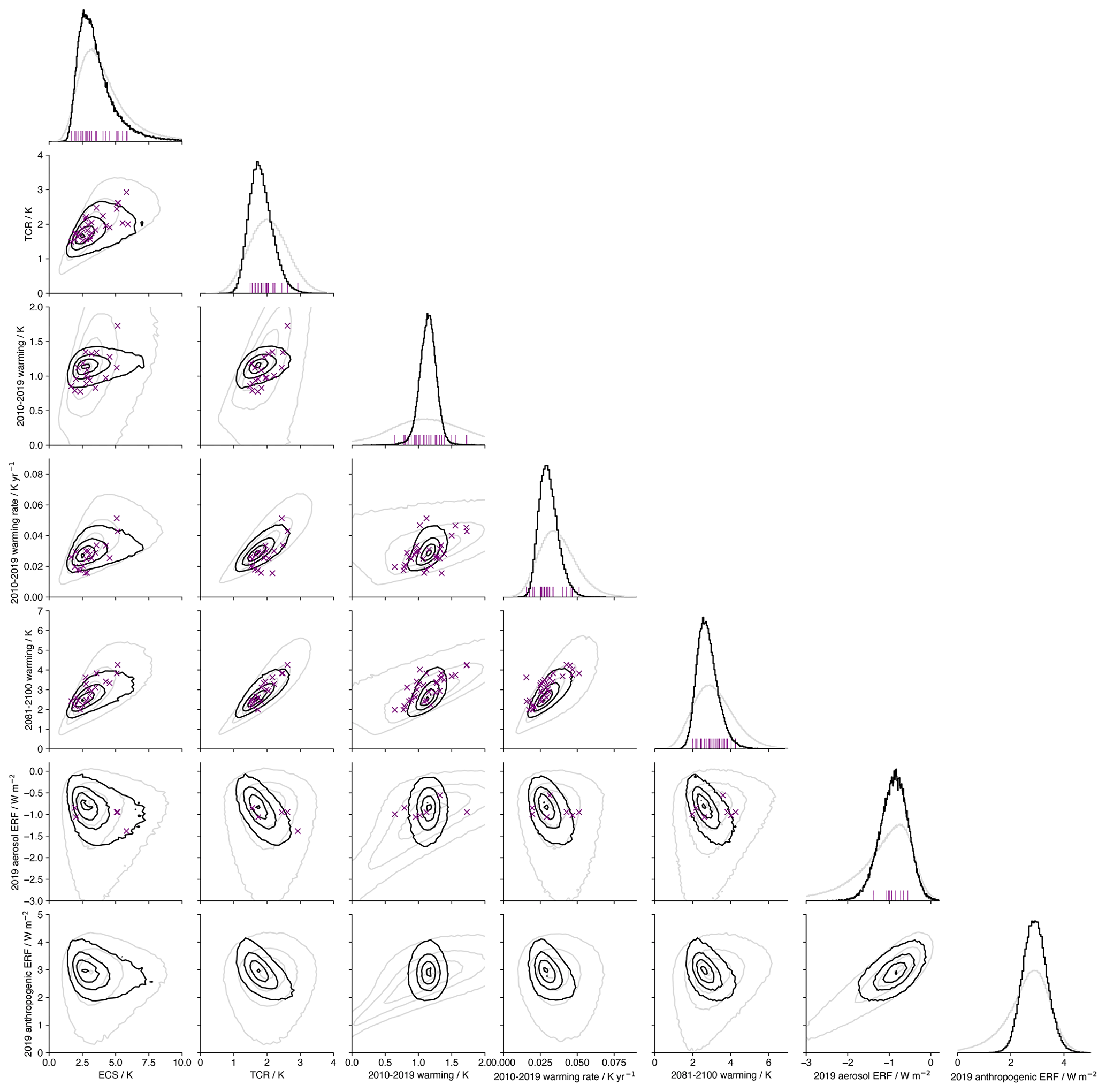
Figure 7 Corner plot of key quantities within the full and constrained ensembles, based on following a historical trajectory to 2014 and SSP2-45 thereafter. Diagonal plots show marginal probability density functions of each key variable: full is shown in grey, and constrained is shown in black. Sub-diagonal plots show contour plots of joint probability density function. Contours shown indicate normalized likelihoods of 5 %, 33 %, 66 %, and 95 %. Purple crosses and lines indicate the positions of individual CMIP6 models. The 2010–2019 warming rate for CMIP6 models is calculated as the slope of a linear regression over 2000–2029 due to internal variability projecting strongly on the slope estimate and error if a shorter period is used.

4.3.4 Sensitivity to prior response parameter distributions

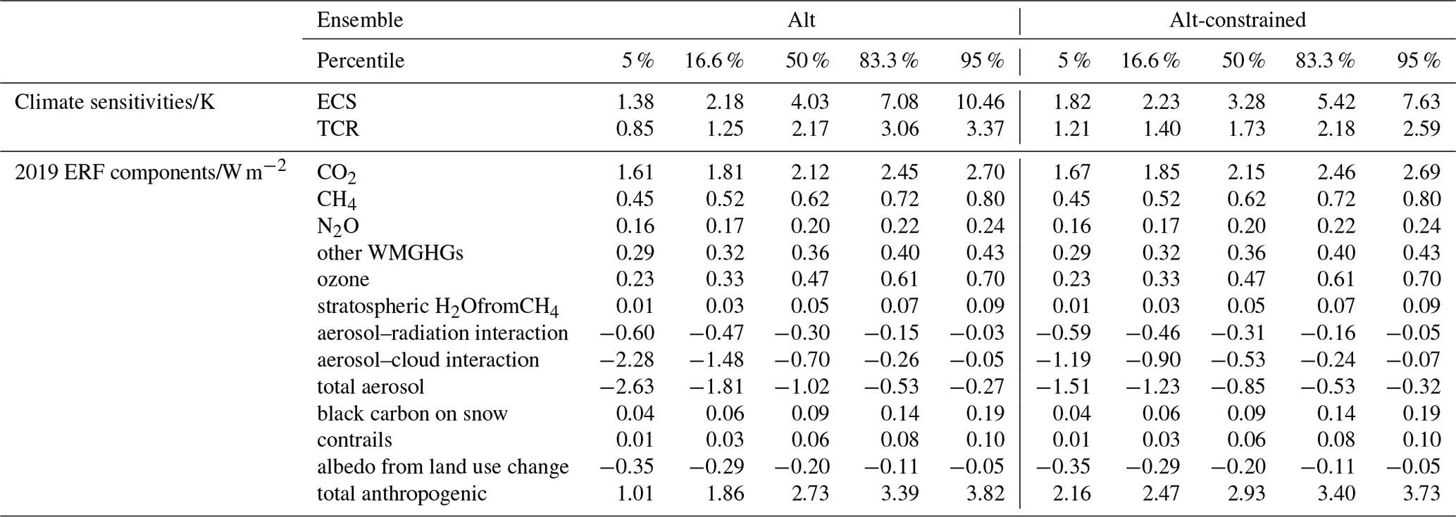
Previous work has shown that posterior marginal distributions of ECS and TCR depend strongly on the assumed prior distributions (Bodman and Jones, 2016). Here we test the sensitivity of our constrained results to the response parameters sampled in FULL by replacing the TCR and RWF sample distributions stated in Sect. 4.2.3 with: $\text{TCR}\sim \mathcal{U}\left(\mathrm{0.5},\mathrm{3.5}\right)$ and $\text{RWF}\sim \mathcal{U}\left(\mathrm{0.2},\mathrm{0.85}\right)$. The actual prior distributions of TCR and RWF differ slightly from those stated here due to the rejection of unphysical response parameter sets, which tends to occur more often for lower values of TCR and higher values of RWF: the quantiles of the “alt” input TCR and ECS distributions are 2.17 [0.85, 3.37] and 4.03 [1.38, 10.46], respectively. The posterior distributions of TCR and ECS after applying the constraint (alt-constrained) described in Sect. 4.1 are 1.73 [1.21, 2.59] and 3.28 [1.82, 7.63]. The resulting marginal posterior distributions are wider than in the constrained ensemble, though not considerably so for the TCR estimate. The upper end of the alt-constrained ECS distribution is most affected by the change in prior, suggesting that the current level and rate of warming does not provide an exceptionally tight constraint on the upper bound of the ECS. The alt-constrained TCR distribution is not significantly different from constrained, differing only by 0.1 K over the range of the distribution, demonstrating the close relationship between the TCR and historical warming (Sanderson, 2020) that enforces a tight constraint even with a significantly less informed prior. Full results from the alt-constrained ensemble are provided in Table 8.

Table 8 Results for the key metrics under a less-informed climate sensitivity prior.

4.3.5 Sensitivity to observational dataset

As stated in Sect. 4.1, the choice of observational dataset used in the Global Warming Index calculation may project significantly onto our results. Here we carry out an identical constraining procedure to that described in Sect. 4.3 but with the distribution of present-day level or rate calculated for each observational product in turn. Constrained values of the ECS, TCR, and projected 2100 warming under an SSP2-45 pathway are shown in Table 9. This sensitivity analysis demonstrates how important the chosen observational dataset is: projections under an SSP2-45 pathway can vary by over 0.2 K depending on the dataset used to determine the constraint.

Table 9 Sensitivity of results for the key metrics to the choice of observational dataset used in the Global Warming Index calculation.

4.4 Constrained idealized experiments

Here we carry out standard CMIP6 experiments used in diagnosing the key properties of the climate – the abrupt-4xCO2 and 1pctCO2 experiments – with the full and constrained parameter ensembles. This represents a test of whether our parameter sampling methods are sufficient to ensure that the range of carbon cycle and climate system responses are sampled from (as informed by the CMIP6 ensemble). We see in Fig. 8a and b that the full 90 % credible interval spans the CMIP6 model ensemble range, though it has a longer lower tail. The full ensemble also spans the range of carbon cycle behaviour in 11 C4MIP models on decadal timescales in Fig. 8d, e, and f, including radiation feedbacks (Arora et al., 2020, Fig. 8g). The constrained ensemble, as expected from the climate sensitivity results in Sect. 4.3, is significantly less spread than the CMIP6 model ensemble. It precludes both models with high and low climate sensitivities. Although our constraint does not significantly affect the carbon cycle parameters, it does preclude some full ensemble members with a high airborne fraction, which becomes more apparent towards the end of the experiments. The constrained ensemble implies a likely range (Fig. 8c) for the (CO₂-only) TCRE (Matthews et al., 2009; Allen et al., 2009; Zickfeld et al., 2016; MacDougall, 2016) of 1.27–1.85, with a central estimate of 1.53 and 5 %–95 % range of 1.11–2.12 K TtC⁻¹, based on the temperature response at a cumulative CO₂ emission of 1000 GtC. The slight non-linearity in the temperature–cumulative emission relationship results in the best-estimate instantaneous TCRE reducing by around 15 % per additional 1000 GtC. These estimates are consistent with recent estimates based on the observational record (Millar and Friedlingstein, 2018; Gillett et al., 2013), though our best estimate is slightly higher and the range is less spread out. This tighter range may be due to the noise reduction from using an idealized experiment and model with no representation of internal variability. It is important to note that our TCRE estimates hold the same sensitivity to the choice of observational dataset used in the Global Warming Index calculation as the TCR (Table 9).

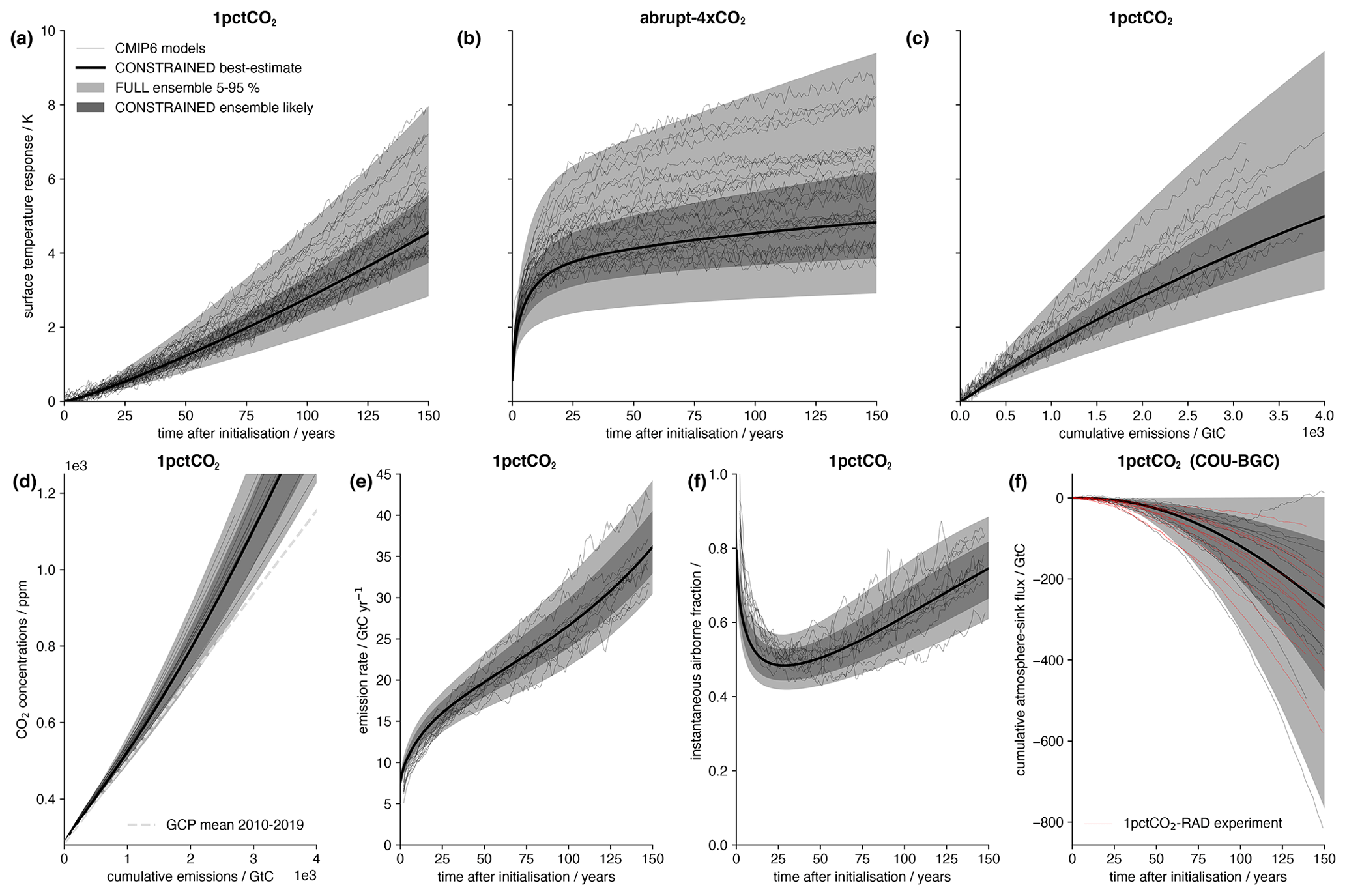
Figure 8 Idealized CMIP6 experiments with full and constrained FaIRv2.0.0-alpha ensembles. Thin black lines show drift-corrected CMIP6 model data. Light grey shading indicates the full ensemble 5 %–95 % range. Dark grey shading indicates the constrained ensemble likely (17 %–83 %) range. The thick black line shows the central constrained series. The dashed grey line in (d) shows the airborne fraction for the most recent decade estimated from the most recent Global Carbon Budget (Friedlingstein et al., 2020), calculated by dividing the atmospheric carbon flux by the mean CO₂ emission rate over this period (see Friedlingstein et al., 2020, Fig. 9). Thin red lines in (g) show data directly from the radiatively coupled C4MIP experiment, while thin black lines show an estimate of the radiation feedback on carbon sink strength as the difference between the fully and biogeochemically coupled C4MIP experiments.

4.5 Constrained scenario projections

We use our CONSTRAINED parameter ensemble to project end-of-century warming and ERF in FaIRv2.0.0 for each SSP (Riahi et al., 2017). In Figs. 9 and 10, we also compare our constrained FaIRv2.0.0 projections to the default setup of MAGICC7.1.0-beta. The two models exhibit some notable differences, particularly in radiative forcing projections due to aerosol emissions and ozone concentrations. For a complete comparison of the constrained ensemble with the probabilistic setup of MAGICC7, see Nicholls et al. (2021).

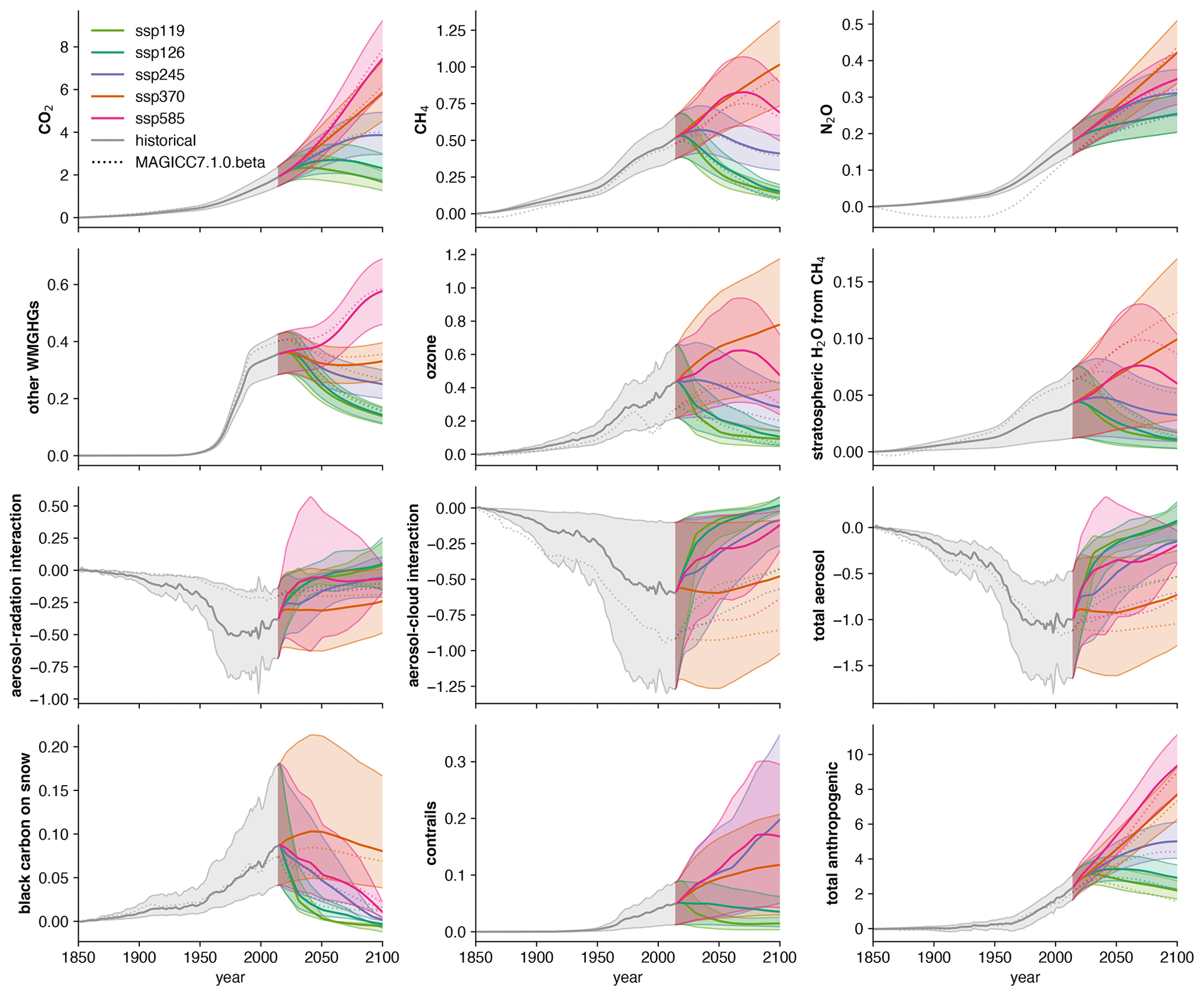
Figure 9 ERF time series (in W m⁻²) by category for a range of SSP pathways using the FaIRv2.0.0-alpha constrained ensemble. Solid lines indicate central estimate, and shading shows the 5 %–95 % range. Dashed lines show default projections from MAGICC7.1.0-beta from RCMIP (Nicholls et al., 2020a).

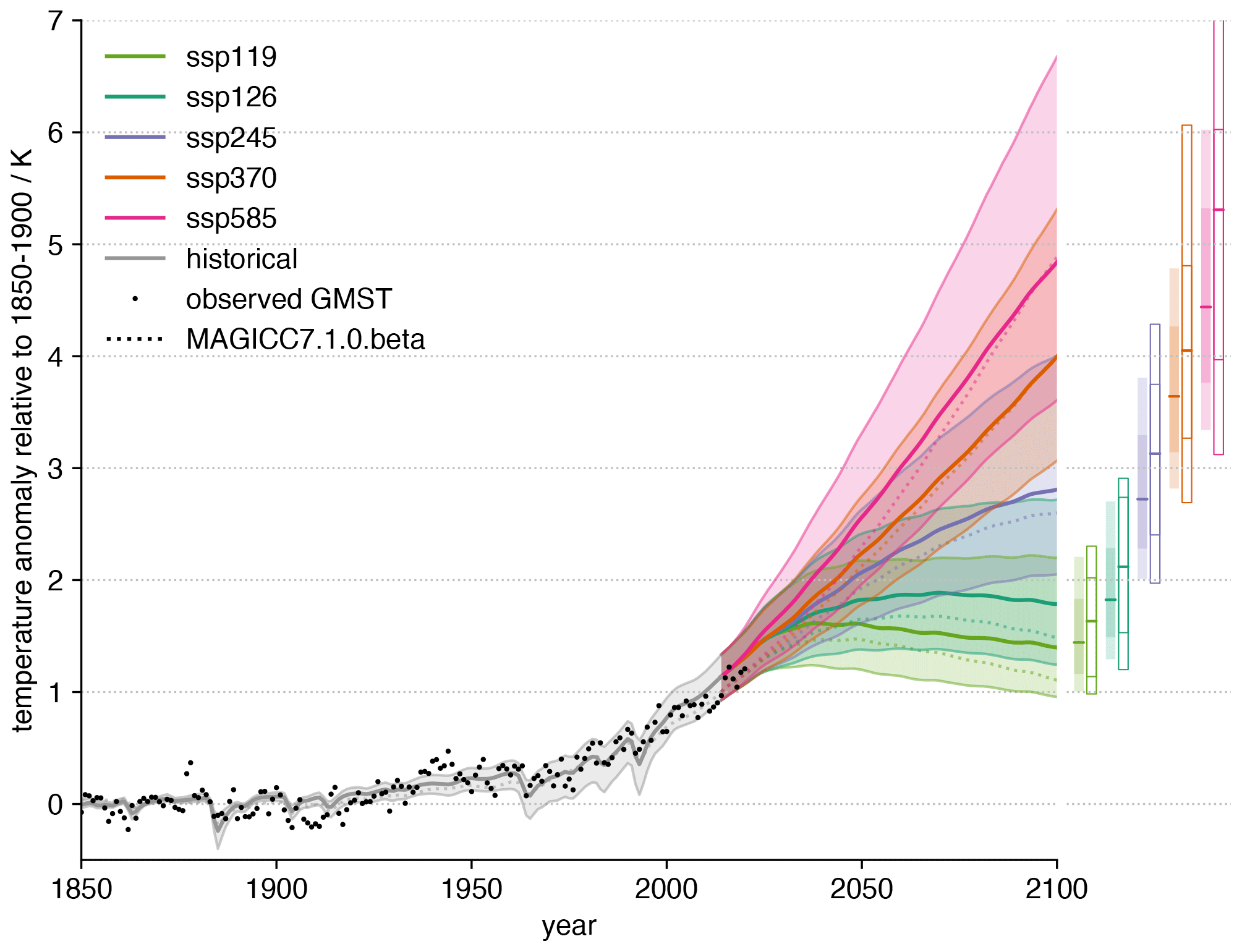
Figure 10 Surface temperature response projections for a range of SSPs with the FaIRv2.0.0-alpha constrained ensemble. Solid lines indicate the central projection. Shading indicates a 5 %–95 % range. The dashed line indicates default projection from MAGICC7.1.0-beta from RCMIP (Nicholls et al., 2020a). Dots show the mean of six observational datasets. Bars on the right-hand side of the figure show end-of-century (2081–2100) warming. Filled bars show the constrained best estimate and likely and 5 %–95 % ranges. Unfilled bars show the CMIP6 median and likely and minimum–maximum range. The number of CMIP6 models used in each scenario is given in Table S4.

The apparent slight warm bias at the present day arises due to a combination of natural variability, in particular the so-called “hiatus” period (Trenberth and Fasullo, 2013), and a too high response to natural forcings. As the constrained ensemble is selected on the basis of the contributions of anthropogenic forcings to global warming only (via the anthropogenic warming index), any bias in the response to natural forcings will project onto the total temperature response. Although the estimated contribution of natural forcings to the present-day level of warming is observational dataset dependent, the mean contribution over all six datasets calculated within our global warming index methodology (i.e. scaled by the optimal fingerprinting regression coefficients) is 0.03 K lower than within our constrained ensemble relative to the 1850–1900 baseline period, suggesting that the climate response to natural forcings is slightly too high. This could be resolved by scaling the prescribed natural forcing data (Smith, 2020) by the average estimated optimal fingerprinting coefficient. However, we do not do this here, instead using the raw data for transparency. The selected 1850–1900 baseline period exacerbates this high response due to the significant volcanic activity during this period.

The projections of future warming are comparable to other recent studies that have used various methodologies to constrain future warming (Brunner et al., 2020; Tokarska et al., 2020; Ribes et al., 2021). Overall, our central estimates agree very well with Tokarska et al. (2020); Ribes et al. (2021), lying a little below those from Ribes et al. (2021). The lower quantiles of our projections generally lie between the estimates from Tokarska et al. (2020) and Ribes et al. (2021). Our upper quantiles (specifically 95 %) agree well with the estimates given in Ribes et al. (2021). Overall, we find that our projections are comparable to other recent studies, though in general they are a little less tightly constrained. Here we have used one relatively straightforward methodology to perform these constrained projections, but we expect that it would be possible to constrain these further through the use of more sophisticated methods or by adding in additional information to the constraint (such as the present level of CO₂ concentrations or an estimate of the total ocean heat uptake – though this would require the energy balance model formulation of the FaIRv2.0.0 climate response to be used). A reasonable next step to improve the probabilistic projections from FaIRv2.0.0 might be to switch to a Markov chain–Monte Carlo approach, as used by other SCMs (Meinshausen et al., 2011b, 2020).

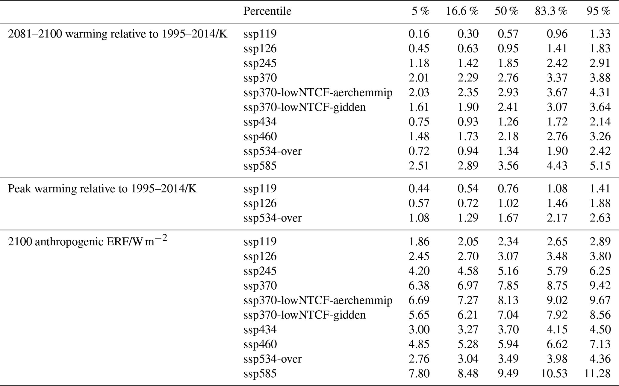
Table 10 Global warming and radiative forcing projections from the FaIRv2.0.0-alpha constrained ensemble under the SSPs. Table S6 in the Supplement displays these warming projections relative to a pre-industrial baseline of 1850–1900.

5 The response of simple climate models

The IPCC Special Report on 1.5 ^∘C warming (IPCC, 2018) included results from two SCMs, FaIRv1.3 (Smith et al., 2018) and MAGICC6 (Meinshausen et al., 2011a). One point of discussion following the report was the difference in results between these two models, with FaIRv1.3 tending to project a lower temperature response than MAGICC6 (Huppmann et al., 2018). This has resulted in a widely held belief that FaIRv1.3 is intrinsically “cooler” than MAGICC6 in general, a belief that some of these authors have unintentionally previously contributed to (Leach et al., 2018). This belief is unfounded: the response of an SCM is a function of the parameters used. Although some parameters may be chosen to be consistent with geophysical observation or theory, in general SCM parameters are tuned such that they emulate or reproduce either the output of more complex models or observations of the Earth. Relating this to the models used in SR15, the FaIRv1.3 ensemble was tuned such that the model response lay within observed changes in global mean surface temperature since the pre-industrial period (Smith et al., 2018; Cowtan and Way, 2014); the MAGICC6 ensemble was constrained to observations up until 2009 (Meinshausen et al., 2009). The two different tuning targets naturally lead to differences in the response of FaIRv1.3 and MAGICC6. Here we emphasize that the differences between the models' output is not systematic – it is the parameters used and how these are selected (which is often a subjective decision on the part of the modellers) that determines the model response.

6 Uses of FaIRv2.0.0

We envisage that FaIRv2.0.0 will primarily be used for similar assessments to those carried out with current SCMs. One advantage that FaIRv2.0.0 has is that it was built with performance in mind and hence is easily vectorized. It can be vectorized in a programming language designed for array operations (such as Fortran, MATLAB, or the NumPy Python module) and hence FaIRv2.0.0 is extremely quick to run. For example, using the alpha Python implementation, FaIRv2.0.0 can compute the million-member full ensemble (emission driven for 52 gases, 81 forcing components, over the period 1750–2100) in under 40 min³. This speed provides significant advantages when computing large probabilistic ensembles or when optimizing parameters. An important consideration for users computing probabilistic ensembles will be the memory required by FaIRv2.0.0 output, as this is more likely to be the limiting factor on a modern computer rather than the model runtime. A related point is that the minimal equation set that FaIRv2.0.0 is composed of is easily transcribed into other programming languages. Although we would recommend using the official Python FaIR release (https://github.com/OMS-NetZero/FAIR, last access: 19 May 2021) where possible, there are many cases where it might be required for FaIRv2.0.0 to be converted into another language (such as GAMS) for use in integrated assessment models. We believe that the relative simplicity of FaIRv2.0.0 lends itself to this purpose. Of particular note is that FaIRv2.0.0, in its entirety, is able to be run in Excel. This opens up climate system exploration and experimentation to a large group of potential users who are familiar with spreadsheets but not programming languages. The user base of Excel is estimated to be around 100 times larger than that of Python (https://info.cambridgespark.com/latest/python-vs-excel, last access: 19 May 2021). To aid with implementation in alternative languages where required, we have provided a brief set of notes on our own Python implementation of the development version of FaIRv2.0.0 in the Supplement.

In terms of possible academic uses of FaIRv2.0.0, we have demonstrated two of the main ones: emulation of more complex models and probabilistic scenario projections. FaIRv2.0.0 can be used to rapidly investigate differences between ESMs by tuning FaIRv2.0.0 to emulate these complex models and comparing differences between the tuned parameter sets to identify which aspects of the models differ most, as was done with MAGICC in Meinshausen et al. (2011a, b). The ability to tune FaIRv2.0.0 to more complex models, as demonstrated here and in other work (Tsutsui, 2017; Joos et al., 2013; Millar et al., 2017), also allows for estimation of complex model response to a particular scenario or experiment without having to expend computer power to run the model itself, which could allow climate system uncertainties to be introduced more fully into integrated assessment studies by emulating the full CMIP6 ensemble within IAMs (providing some of the capability demonstrated by Meinshausen et al. (2011a), with a simpler model). The probabilistic scenario projection we demonstrated in Sect. 4 is a potentially more policy-relevant academic use of FaIRv2.0.0, since CMIP6 model emulations do not necessarily represent the best estimate of some key properties of the real-life Earth system when historical observations are taken into account (Tokarska et al., 2020; Gillett et al., 2021). The speed of FaIRv2.0.0 allows very large parameter ensembles to be run rapidly, enabling all regions of plausible parameter space to be explored without requiring large quantities of computing resources. Although we have performed one relatively simple methodology for the creation of an observationally constrained large ensemble here, there are many possible ways to do this, for example using the Markov chain–Monte Carlo methods employed in several other SCMs (Nicholls et al., 2020b; Meinshausen et al., 2020, 2011b). A third academic use of FaIRv2.0.0, which we are interested in, is its incorporation into integrated assessment models (IAMs). Its simplicity and computational efficiency may make implementation within existing IAMs relatively more straightforward than for other SCMs, even if the whole model is required to be built up from scratch in whatever format would be required by the particular IAM.

Outside of academia, we propose that FaIRv2.0.0 could be used for emission climate impact accounting in industry. The UNFCCC standard for the reporting of greenhouse gas emissions is to account for emissions of all gases as a CO₂ equivalent quantity via the 100-year global warming potential (GWP). However, GWPs do not adequately capture the behaviour of short-lived climate pollutants such as methane (Cain et al., 2019), leading to the development of alternative metrics such as GWP*. We suggest that such warming impacts could potentially instead be simulated using a simple climate model as an improvement upon the use of any of these metrics. Although this does represent a step-up in complexity, we believe that the relative simplicity of FaIRv2.0.0, when compared to other SCMs, makes it a strong candidate for this usage. In particular, the ability of FaIRv2.0.0 to be run in Excel could encourage this particular use case. We suggest that the speed, simplicity, and transparency of FaIRv2.0.0 also lends it to use in undergraduate and high-school education. It can be used to explain (and demonstrate) important features of both the carbon (or other GHG) cycle and Earth's thermal response to radiative forcing and is simple enough to use that students could themselves carry out experiments (such as a CO₂ doubling) easily with no prior experience and only basic computing skills.

7 Conclusions

In this paper we have presented a significant update to the FaIR SCM (Smith et al., 2018), focussed on reducing the structural complexity of the model as much as possible. The updated model, FaIRv2.0.0, uses the five equations of the AR5 impulse response model (Myhre et al., 2013) plus just one additional equation to allow the model to represent non-linearities in the carbon cycle. We demonstrate that this reduction in complexity does not come at the cost of the model's ability to reproduce globally averaged observations or output of more complex models from CMIP6 (Eyring et al., 2016). After demonstrating the ability of the model in emulating more complex models, we show how the model can be used for climate projection by constraining a large parameter ensemble.

There are many potential uses for FaIRv2.0.0 as a result of its simplicity and transparency. In addition to being available for the same probabilistic scenario assessment as is carried out by SCMs in reports such as SR15 (IPCC, 2018), it could be implemented into IAMs and would likely improve computational efficiency due to its vectorization and resulting extremely rapid runtime. We encourage policymakers to use FaIRv2.0.0 in order to directly assess whether warming implications are aligned with the intended outcomes of mitigation policies, since GHG accounting metrics used at present such as GWP do not provide accurate results for targets such as net-zero CO₂ due to the short life of some GHGs (Allen et al., 2018). To aid this use of FaIRv2.0.0, we will provide an Excel file containing the model with its default parameter set, ensuring FaIRv2.0.0 is available for all interested parties, even those unfamiliar with computer programming languages. The Excel version of the model could also be used to assist teaching of climate change and climate processes and could even allow students access to an easy-to-understand model that they could use themselves to explore future scenarios and the relative impacts of future emissions of different greenhouse gases or demonstrate the importance of climate sensitivity in an interactive manner.

FaIRv2.0.0 sits at the very low end of complexity within the broad spectrum of currently available simple climate models. It is a very highly parameterized model for simulating globally averaged relationships between greenhouse gas and aerosol emissions, atmospheric greenhouse gas concentrations, radiative forcing, and surface temperature response. We have shown that despite its simplicity, it is able to span the wide range of behaviours exhibited by much more complex models and those inferred from observations. In addition, we have provided some basic comparisons to both the previous version of FaIR(v1.5) and the widely used MAGICC SCM (Meinshausen et al., 2011a, b, 2020). More detailed comparisons are outside the remit of this paper, but RCMIP (Nicholls et al., 2020b, a) covers this topic comprehensively. We expect that FaIRv2.0.0 is very close to as simple as an SCM could get without losing a significant proportion of this representation ability. However, it does not explicitly simulate the physical processes behind these variables, which may preclude it from some applications where other, more complex SCMs such as MAGICC would be usable. Overall, however, we hope that FaIRv2.0.0 will be an important contribution to the available set of SCMs given its wide range of potential use cases and that it will open up climate system modelling to a wide range of novel users in both industry and education.