the Creative Commons Attribution 4.0 License.
the Creative Commons Attribution 4.0 License.
 | 19 Jan 2021
FORTE 2.0: a fast, parallel and flexible coupled climate model
Manoj Joshi
Bablu Sinha
David P. Stevens
Robin S. Smith
Joël J.-M. Hirschi
FORTE 2.0 is an intermediate-resolution coupled atmosphere–ocean general circulation model (AOGCM) consisting of the Intermediate General Circulation Model 4 (IGCM4), a T42 spectral atmosphere with 35σ layers, coupled to Modular Ocean Model – Array (MOMA), a 2∘ × 2∘ ocean with 15 z-layer depth levels. Sea ice is represented by a simple flux barrier. Both the atmosphere and ocean components are coded in Fortran. It is capable of producing a stable climate for long integrations without the need for flux adjustments. One flexibility afforded by the IGCM4 atmosphere is the ability to configure the atmosphere with either 35σ layers (troposphere and stratosphere) or 20σ layers (troposphere only). This enables experimental designs for exploring the roles of the troposphere and stratosphere, and the faster integration of the 20σ layer configuration enables longer duration studies on modest hardware. A description of FORTE 2.0 is given, followed by the analysis of two 2000-year control integrations, one using the 35σ configuration of IGCM4 and one using the 20σ configuration.
- Article
(24603 KB) - Full-text XML
-
Supplement
(36577 KB) - BibTeX
- EndNote


Numerical models of the coupled (atmosphere–ocean) climate system are important tools for studying the Earth's climate. They provide insight into phenomena which are difficult to observe directly, such as the Atlantic Meridional Overturning Circulation (AMOC) or the effects of increasing atmospheric CO2. They can also be used to test hypotheses about the global climate and the world we live in. In a climate model, it is possible to study the climate response to extreme events such as loss of ice cover (and the resulting change in albedo). Whilst the results in terms of quantitative changes to temperature, precipitation and other climate variables should be treated with caution, it is possible to examine the processes which lead to the predicted changes.
There is a broad spectrum of coupled climate models. At one end of the spectrum are coarse-resolution simplified models designed to run millennial-scale experiments quickly and for minimal computational cost, both in terms of computing power and memory resources (e.g. GENIE, Marsh et al., 2007; CLIMBER, Montoya et al., 2005; UVic, Weaver, 2004; ECBilt, Haarsma et al., 1996). At the opposite end of the spectrum, high-resolution (<0.1–0.5∘ ocean) models (e.g. those contributing to the CMIP6 HighResMIP, Haarsma et al., 2016, such as HadGEM3-GC3.1, Roberts et al., 2019, and HiGEM, Shaffrey et al., 2009). Between the two extremes are the intermediate-resolution models (e.g. HadCM3, Gordon et al., 2000; FAMOUS, Smith et al., 2008), including most of the coupled climate models contributing to CMIP3 (Meehl et al., 2007), CMIP5 (Taylor et al., 2012) and CMIP6 (Eyring et al., 2016). It is worth noting that model development does not equate solely to an increase in horizontal resolution. Inclusion of more, or better parameterised, Earth system processes can be an equally if not more important development (e.g. Sellar et al., 2019).
Sinha and Smith (2002) developed FORTE (Fast Ocean Rapid Troposphere Experiment), a fast and flexible coupled climate model, for the purposes of climate studies. FORTE's speed and flexibility meant that the original model was an ideal educational and research tool. The flexibility of FORTE is evident in the variety of experiments in which it has been used to study ocean and/or climate phenomena. Examples include Buchan et al. (2014), in which observed sea surface temperature (SST) anomalies from 2009 to 2010 were applied to the model SST field prior to the coupling time step, enabling the authors to examine the effect of observed SST anomalies in an otherwise free-running coupled model; in Sinha et al. (2012), the simplicity of FORTE made it easy to examine the effect of orography on the AMOC; Wilson et al. (2009) used the flexibility to examine the roles of orography and ocean dynamics on atmospheric storm tracks, performing experiments with either an interactive ocean or the static mixed layer option in the Intermediate General Circulation Model (IGCM) atmosphere; Blaker et al. (2006) added initial condition perturbations to the Southern Ocean to study fast ocean teleconnection processes; and Atkinson et al. (2009) performed similar experiments using both ocean-only and coupled configurations. Although most studies used FORTE with a T42 resolution atmosphere and 2∘ ocean, a version of FORTE using a T21 resolution atmosphere and 4∘ ocean has also been used for idealised experiments featuring Pangean and aquaplanet configurations (e.g. Smith et al., 2004, 2006). Simulations of FORTE have also been analysed in other climate studies (Hunt et al., 2013; Grist et al., 2008). However, until now, there has been no comprehensive, peer-reviewed publication describing the model itself.
A new version of the atmosphere component of FORTE was released in 2015, and a desire to perform coupled experiments once again resulted in a refresh of FORTE. To avoid confusion with earlier endeavours but at the same time make clear the ancestry of the model, we decided to refer to the refreshed model as FORTE 2.0. This paper describes the coupled model and its components and demonstrates that FORTE 2.0 produces a realistic and stable climate without the need for flux adjustments. The control integrations described are 2000-year integrations starting from rest with the Levitus (temperature, salinity) climatology (Levitus and Boyer, 1998; Levitus et al., 1998) and pre-industrial atmospheric concentrations of CO2. The model is forced solely by incoming solar radiation at the top of the atmosphere. The rest of this paper is organised as follows: Sect. 2 gives a description of FORTE 2.0; Sect. 3 presents the model spin-up; Sect. 4 presents the control climate; Sect. 5 discusses the main modes of climate variability in the model; Sect. 6 concludes the paper.
FORTE 2.0 is a global coupled atmosphere–ocean general circulation model consisting of a 2∘ resolution configuration of the MOMA (Modular Ocean Model – Array) (Webb, 1996) ocean model coupled to a T42 (approximately 2.8∘) configuration of the IGCM4 (Joshi et al., 2015) atmosphere model. FORTE 2.0 is an updated incarnation of FORTE (Fast Ocean Rapid Troposphere Experiment) (Sinha and Smith, 2002; Smith et al., 2004), with the most significant changes being an increase in horizontal resolution of both the ocean and atmosphere components by a factor of 2 and an update of the atmosphere code from IGCM3 (Forster et al., 2000) to IGCM4 (Joshi et al., 2015).
The ocean and atmosphere components of FORTE 2.0 are coupled once per model day using OASIS version 2.3 (Terray et al., 1999) and PVM version 3.4.6 (Parallel Virtual Machine; see http://www.csm.ornl.gov/pvm/, last access: 18 November 2020, Geist et al., 1994). Daily average quantities of the variables that are to be exchanged are stored in arrays, and at the end of each model day these are passed to the coupler. MOMA provides daily mean values of sea surface temperature, zonal and meridional velocities, whilst IGCM4 provides solar and non-solar heat fluxes, net freshwater flux, and zonal and meridional surface wind stress. Interpolation between the ocean and atmosphere grids is performed by the coupler using a pre-computed set of weights to ensure conservation.
Integration is relatively fast (∼100 model years per wall-clock day on a 28-core 2.4 GHz Intel Broadwell CPU), and the model can be run on a desktop computer, making it ideal for experiments where more complex higher-resolution models are resource limited. The retention of the full primitive equations for fluid flow in both atmosphere and ocean allows more realistic simulations than possible with Earth models of intermediate complexity (EMICs). In addition, FORTE 2.0 is readily configurable, allowing experiments with realistic and idealised configurations of coastlines, orography and ocean bottom topography.
2.1 The atmosphere component
The atmosphere component of FORTE 2.0 is IGCM4 (Joshi et al., 2015), run with a T42 spectral resolution. A longitudinally regular and Gaussian in latitude grid with a grid spacing of 2.8∘ is used for advection and diabatic processes. The resolution is sufficient to enable stable climate integrations without the need for flux adjustments. There are two pre-configured choices for the number of vertical levels: a troposphere-only atmosphere represented by 20σ levels (L20) which extends to around 25 km altitude or a 35σ level configuration (L35) which includes the stratosphere and extends to around 65 km altitude. To avoid issues with 2Δz oscillations under certain conditions, the NIKOSRAD radiation scheme in IGCM3 (used previously in FORTE) was replaced with a modified version of the Morcrette radiation scheme (Zhong and Haigh, 1995). For further details of the IGCM4 and its performance, we refer the reader to Joshi et al. (2015) and references therein. The model is run with 96 (L35) or 72 (L20) time steps per day. Orography is derived from the US Naval 1∕6th degree resolution dataset. IGCM4 is Message Passing Interface (MPI) parallelised, and at this resolution integration on 16–32 cores achieves the best performance.
Atmospheric convection is dealt with via a Betts–Miller scheme (Betts and Miller, 1993). Low, medium and high layer clouds and convective cloud amounts are represented based on a critical relative humidity criterion (see the Appendix of Forster et al., 2000). The formula which determines low-level cloud amount has an additional factor of 50 % compared to that used by Forster et al. (2000) to correct a cold bias within the tropical ocean which led to unrealistic circulation in the Pacific. In addition to variation with solar zenith angle (and hence latitude), sea surface albedo is increased away from polar regions to compensate for the absence of aerosols which would otherwise scatter incoming solar radiation. Land grid boxes are assigned a vegetation index, one of 24 pre-defined vegetation types, which determine the albedo and roughness length.
Coupling to the dynamic ocean model requires some changes to the surface boundary layer. In order to conserve water, it is necessary to account for soil moisture and implement river runoff. Soil moisture for each land grid box is represented as a bucket, or reservoir, 0.5 m in depth. Excess water, i.e. when the volume of water is greater than the volume of the bucket, is accumulated and added to the ocean as runoff at each coupling time step. The land surface is divided into catchment basins, and the accumulated runoff is distributed on a list of predetermined atmospheric grid cells that lie over the ocean and represent river mouths. The catchment areas and river discharge points are derived from Weaver et al. (1998), as explained in Sinha and Smith (2002). Runoff accumulated over Antarctica is distributed uniformly over the ocean south of 55∘ S, as a simplistic representation of iceberg calving and melting. Additionally, land snow cover is capped at a maximum thickness of 4 m. Excess snow over Antarctica and the Arctic region is treated separately as an additional runoff term that represents iceberg melting and calving. As with the soil moisture, runoff from excess snow over Antarctica is distributed uniformly over the ocean south of 55∘ S. Excess snowmelt over the Arctic is handled similarly, with a uniform distribution over the ocean north of 66∘ N.
A coastal tiling routine is implemented in order to handle the differences between the atmosphere and ocean grids. Grid cells in the ocean are either ocean or land, whilst atmospheric grid cells can be ocean, land or partial (i.e. they extend over both ocean and land cells on the ocean grid). Atmospheric grid cells that wholly overlie ocean are updated using the normal IGCM4 boundary layer scheme and the SST from the ocean model that is exchanged through the coupler. Similarly, cells that wholly overlie land are updated using the IGCM4 land surface scheme. For partial atmosphere grid cells, two sets of boundary layer variables (e.g. latent heat flux) exist. One set is updated like any other land point using the IGCM4 boundary layer scheme, and the other set is updated like any other ocean point. The atmosphere then sees the weighted average of the heat fluxes over the land and sea. Care is taken to ensure that atmospheric moisture is conserved and that precipitation is also apportioned correctly between the land surface scheme and the ocean fraction of the atmosphere cell.
To improve the representation of the effects of sea surface roughness on momentum exchange, a wind-dependent drag coefficient, Cd, is implemented, such that , where U10 is the 10 m wind speed (Wu, 1980). This gives a maximum Cd=0.003 at a wind speed of 40 m s−1 without ice cover. is the drag coefficient over ocean cells, calculated using a globally uniform value for surface roughness over the open ocean.
At present, FORTE 2.0 does not include dynamic sea-ice representation. Instead, sea ice is represented by a barrier to heat fluxes between the ocean and atmosphere components, which is imposed when the sea surface temperature reaches 271 K, and surface albedo is increased to 0.6 to represent ice cover. The albedo continues to linearly increase, reaching 0.8 at 261 K as a means to represent the albedo effects of snow on ice. Once the albedo reaches 0.8, it will not reduce until the temperature rises above freezing point and the flux barrier deactivates. There is no advection of sea ice, and salinity and runoff fluxes remain unaffected. SST under ice is relaxed toward the freezing point of seawater (−1.8 ∘C) on a 10 d timescale.
2.2 The ocean component
The ocean component of FORTE 2.0 is MOMA (Webb, 1996), a version of the Geophysical Fluid Dynamics Laboratory (GFDL) MOM (Modular Ocean Model) (Pacanowski et al., 1990) coded to work more efficiently on array processors, which solves the primitive equations discretised using finite differences on an Arakawa B grid (Arakawa, 1966). It has a linear free surface (Killworth et al., 1991) and uses “full cell” ocean bathymetry. In the configuration used for this integration, the ocean horizontal resolution is 2∘ × 2∘, with 15 z-layer levels, increasing in thickness with depth from 30 m at the surface to 800 m at the bottom. A polar island, comprising the top row of grid cells (88–90∘ N), is required in the Arctic to prevent numerical instability due to convergence of lines of longitude. There are 64 baroclinic time steps per day (22.5 min time steps) implemented using the modified split QUICK (MSQ) advection scheme (Webb et al., 1998). The version of MOMA used in FORTE 2.0 uses OpenMP shared-memory parallelisation, and running it on four to six cores is typically sufficient to match the IGCM4 performance.
Bathymetry is derived from the ETOPO5 (1988) 1∕12∘ resolution dataset, and interpolated onto the model resolution. Due to the horizontal resolution, in order to encourage dense water formation and flow between the Nordic Seas and North Atlantic, bathymetry is manually excavated in a manner similar to HadCM3 (Gordon et al., 2000). The Bering, Gibraltar and Kattegat/Skagerrak straits are represented by a single grid box which, due to the Arakawa B grid, means that there is no advection through them, but diffusion of potential temperature (T) and salinity (S) does occur.
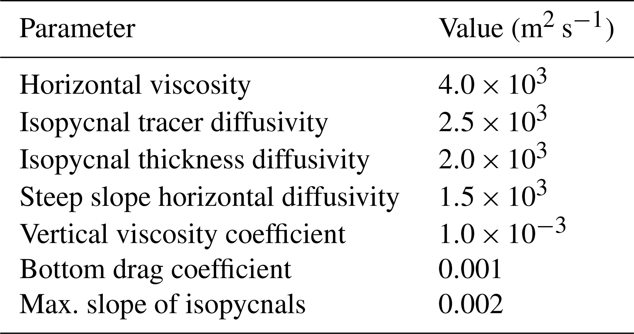
Ocean isopycnal mixing is represented in MOMA through the isoneutral mixing scheme of Griffies et al. (1998). The eddy-stirring process of Gent and McWilliams (1990) is introduced as a skew flux (Griffies, 1998). Where isopycnal slopes become large, exponential tapering scales isoneutral diffusivities to zero as the slope increases (Danabasoglu and McWilliams, 1995). The isopycnal mixing parameters used for the control simulation described in Sect. 3 are shown in Table 1.
To ameliorate some of the shortcomings identified in earlier FORTE simulations, some additional changes have been made to MOMA. Firstly, the background vertical diffusion, κ, is set to be stability dependent (Gargett, 1984), albeit with the surface to sea floor potential temperature gradient as a simple proxy for stability, such that
where Ts is the surface potential temperature, Tb is the bottom potential temperature, z is depth, and H is the local total depth of the ocean. Thus, the vertical diffusivity takes a maximum value of m2 s−1 at the sea floor and at high latitudes, with lower values, approaching m2 s−1 in the upper ocean at low latitudes.
Secondly, starting from 5∘ N/S the horizontal diffusion in the surface layer increases towards the Equator from its default value to 20 times this value at the Equator to counteract equatorial upwelling and, in a simple way, parameterise the eddy heat convergence associated with tropical instability waves which was highlighted by Shaffrey et al. (2009).
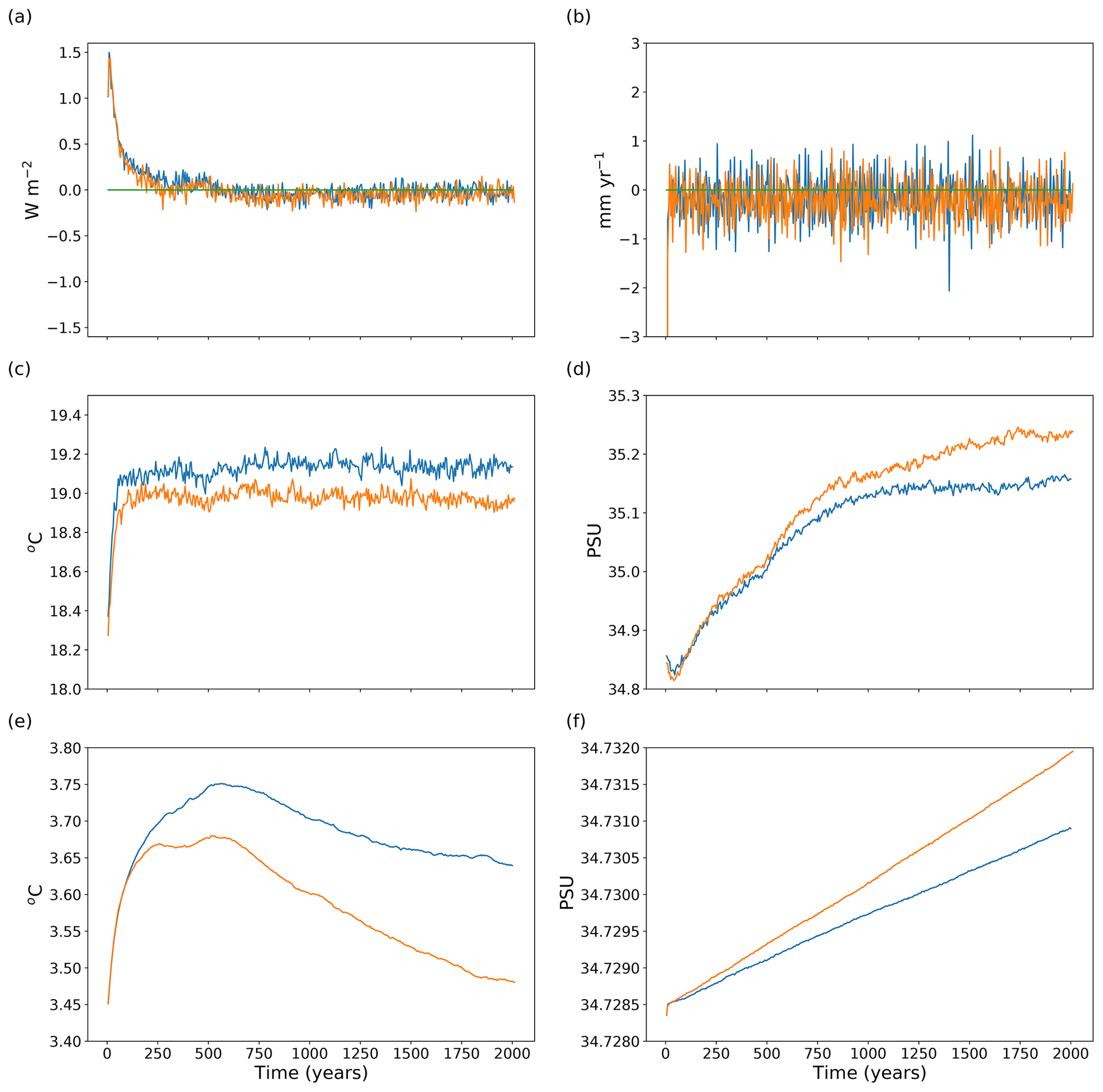
Figure 1Time series of global mean (a) surface heat flux (W m−2) and (b) surface water flux (mm yr−1) into the ocean, (c) SST (∘C) and (d) SSS, and volume-averaged (e) potential temperature and (f) salinity. Cyan and orange lines show the quantities for the simulations run with the L35 and L20 configurations, respectively.
To evaluate the performance of FORTE2.0, we ran a pair of control integrations with pre-industrial CO2 concentration using both the 35σ layer and 20σ layer atmosphere configurations. In each simulation, FORTE 2.0 starts from rest with identical initial ocean temperature and salinity fields from Levitus and Boyer (1998) and Levitus et al. (1998) interpolated onto the ocean model grid. Figure 1 shows area and volume integrated quantities of the surface heat and freshwater fluxes, and ocean temperature and salinity from each of the two integrations. The surface heat flux into the ocean is initially positive (up to 1.5 W m−2) but the imbalance reduces to less than 0.5 W m−2 after a few decades and then stabilises and remains within ±0.2 W m−2 throughout the remainder of the integration (Fig. 1a). The time average water budget closes to within −0.2 mm yr−1, after an initial adjustment in the first year of the integration (Fig. 1b). The global average SST settles within 100 years to values around 19.1 ∘C for the L35 configuration and 19.0 ∘C for the L20 configuration (Fig. 1c). Sea surface salinity (SSS) in both configurations adjusts more slowly, with L35 maintaining a value of around 35.15 PSU after 1000 years of integration and L20 approaching 35.23 PSU towards the end of the 2000-year simulation (Fig. 1d). The mean SST is 0.9 ∘C warmer than the initial state provided by Levitus and Boyer (1998) (18.2 ∘C). The volume average ocean potential temperature warms by 0.3 ∘C for L35 and 0.2 ∘C for L20 over the first 500 years and then cools more steadily, at a rate of approximately 0.005 ∘C per century for L35. After 2000 years, the volume average temperature in the L20 configurations is close to the initial value. Salinity shows a gradual trend of 0.000125 PSU per century after an initial adjustment in L35, which is a reflection of the small imbalance in the freshwater fluxes. The trend in the L20 configuration is around 30 % stronger.
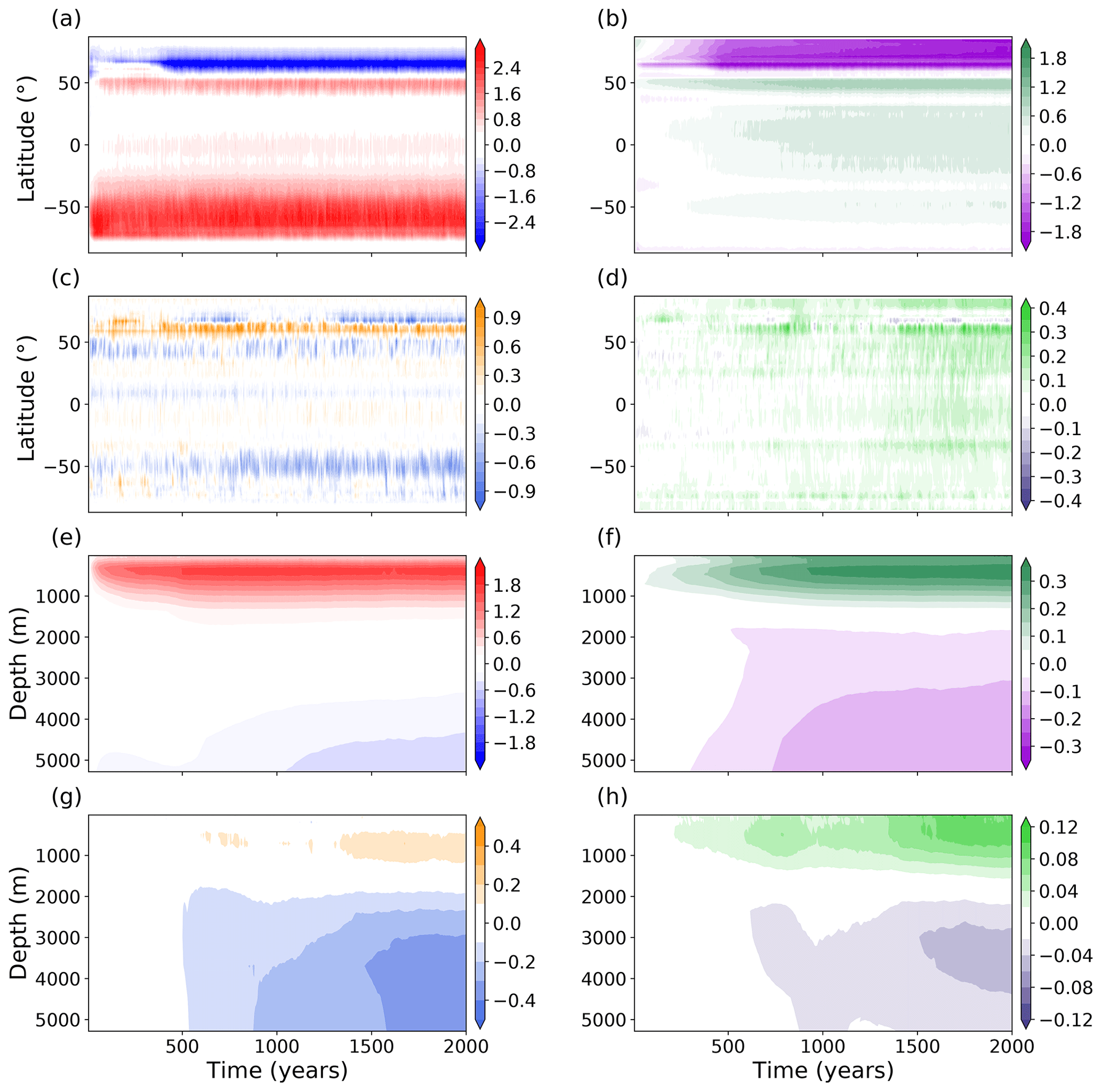
Figure 2Time–latitude plots of drift in annual mean sea surface (a) temperature (∘C) and (b) salinity (PSU) in the L35 simulation. Differences (L20–L35) in annual mean sea surface (c) temperature (∘C) and (d) salinity (PSU). Time–depth series of global drift in annual mean (e) potential temperature (∘C) and (f) salinity (PSU). Differences (L20–L35) in annual mean (g) potential temperature (∘C) and (h) salinity (PSU). Drift is relative to initial conditions.
Global averaged time series of temperature and salinity as functions of latitude and depth are presented in Fig. 2. The time–latitude plots show an initial strong warming of the Southern Ocean that is not density compensated by an increase in salinity at the same latitudes. The onset of this warming occurs quickly and then remains stable for the remainder of the 2000-year integration. A minimal bias develops in the tropical and equatorial regions. In the Northern Hemisphere higher latitudes, there is a strong cooling that (partly) coincides with a freshening. The differences in time–latitude evolution of the SST and SSS for the L20 configuration are shown in Fig. 2c and d. High-latitude SST is slightly cooler in L20 compared with L35, except for a narrow band around 55–65∘ N where a warming of a few tenths of a degree occurs. Surface salinity is marginally higher and to a large extent latitudinally uniform in L20. The difference in SSS is slightly more pronounced at the same latitude range as the narrow band of warming seen in the SSS. Analysis of the spatial SST and SSS biases presented later in this paper shows that these anomalies are located in the Nordic Seas. This pattern develops over the first 500 years of the simulation and then remains stable for the rest of the integration. The SST bias is within the range of that found in the CMIP5 ensemble (Flato et al., 2013).
The time–depth series of potential temperature (Fig. 2e) compares reasonably with those of other, higher-resolution, models such as HadCM3, HadGEM1 and CHIME (Fig. 7 in Johns et al., 2006; Fig. 3 in Megann et al., 2010). FORTE 2.0 warms above 1500 m, with the maximum difference from observed values reaching +1.6 ∘C between 400 and 500 m depth. At depths below 4000 m, the ocean cools initially, with differences from observations at 5000 m reaching −0.2 ∘C. Differences in salinity from observations, again shown as a global averaged time–depth series, are small (Fig. 2f). Differences of +0.3 PSU occur between 300 and 600 m, whilst below 1500 m they are negative and reach a maximum of −0.15 PSU in the abyssal ocean. Differences between L20 and L35 are shown in Fig. 2g and h. L20 exhibits a stronger cooling trend in the deep ocean, such that below 2000 m it is around 0.3 ∘C cooler than L35 after 2000 years. The dipole structure that develops in the time–depth plot of salinity (Fig. 2f) is more pronounced, with the biases at 500 and 3500 m both 25 % stronger in L20 than in L35.
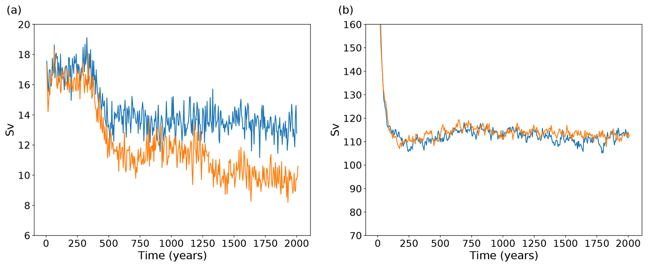
Figure 3Time series of (a) the 5-year mean AMOC and (b) Drake Passage transport in the control integrations. Cyan (orange) lines show transport for the L35 (L20) configuration.
The time series of the maximum AMOC at 30∘ N is presented in Fig. 3. During the first 300 years of integration, a relatively stable 16–18 Sv is maintained in both the L35 and L20 configurations. After 300 years, both configurations undergo a reduction, with the AMOC in L35 reducing by ∼4 Sv to 13–15 Sv. The AMOC in L20 reduces initially by ∼4 Sv and then again around 1250 years into the integration, settling at a value around 10–11 Sv. The weaker AMOC in L20 is consistent with the cooling and freshening trends seen at depth, since a weaker AMOC allows a greater influence of Antarctic Bottom Water (AABW) in the abyssal ocean. The AMOC values in both simulations are maintained for the remainder of the 2000-year integrations and are within the range of those from the CMIP5 ensemble (Heuzé et al., 2015). The standard deviation of the AMOC based on monthly mean values is 3.5 Sv, which is in reasonable agreement with the magnitude of observed variability (McCarthy et al., 2012). Other than the adjustment in the first 500 years, there is little evidence of emergent decadal or multidecadal variability over the course of the L35 control integration, the peak-to-peak range over the last 1500 years of the integration being 3–4 Sv. The initial strong AMOC followed by a reduction after a few centuries is a common feature of FORTE integrations and appears to be linked to a developing fresh bias over the Greenland, Iceland and Norwegian (GIN) seas (shown later).
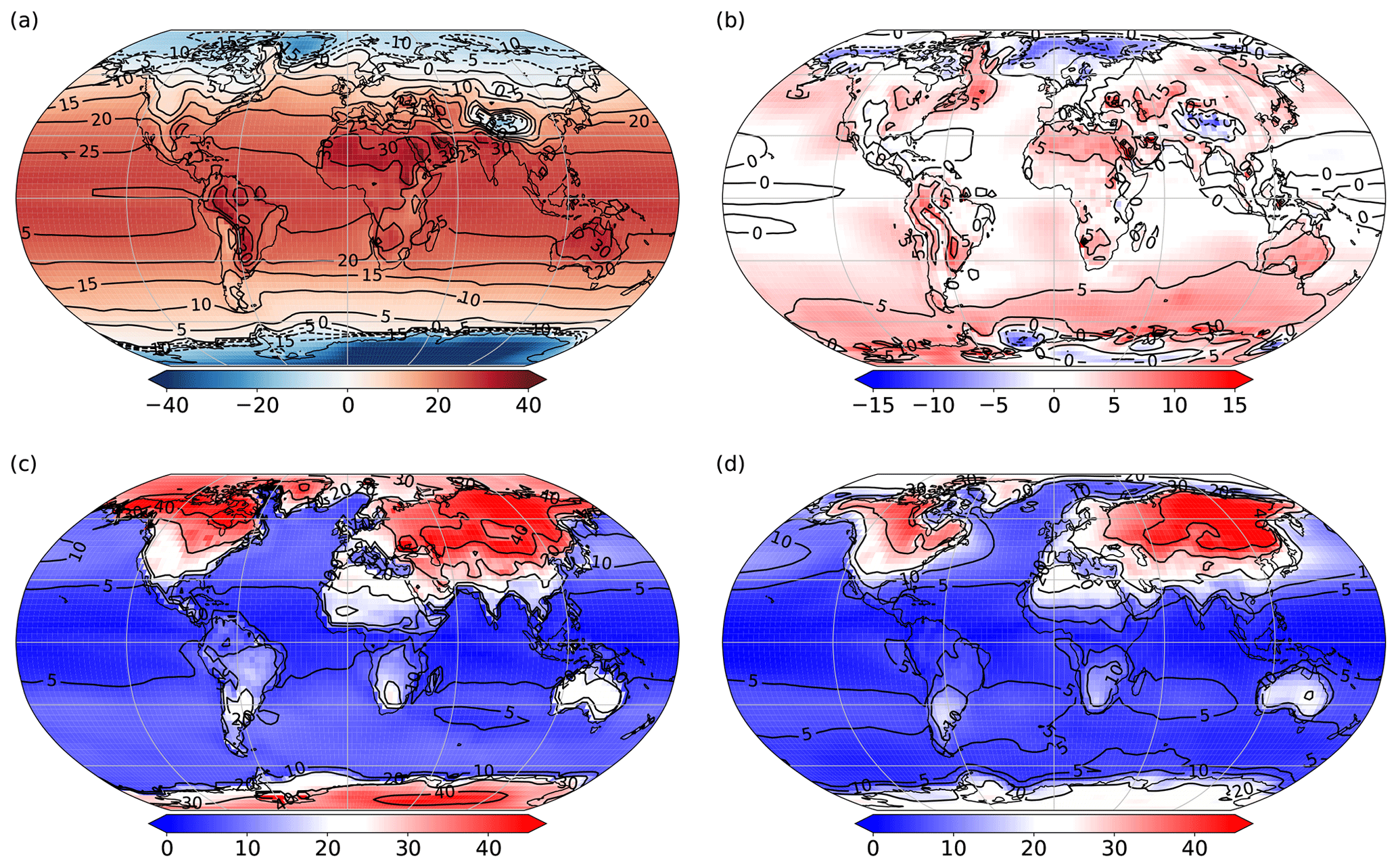
Figure 4Time mean (years 2001–2025) plots from the L35 configuration showing surface air temperature (∘C): (a) annual mean, (b) anomaly from 20CR years 1871–1896, (c) seasonal range in FORTE 2.0 and (d) seasonal range in 20CR years 1871–1896.
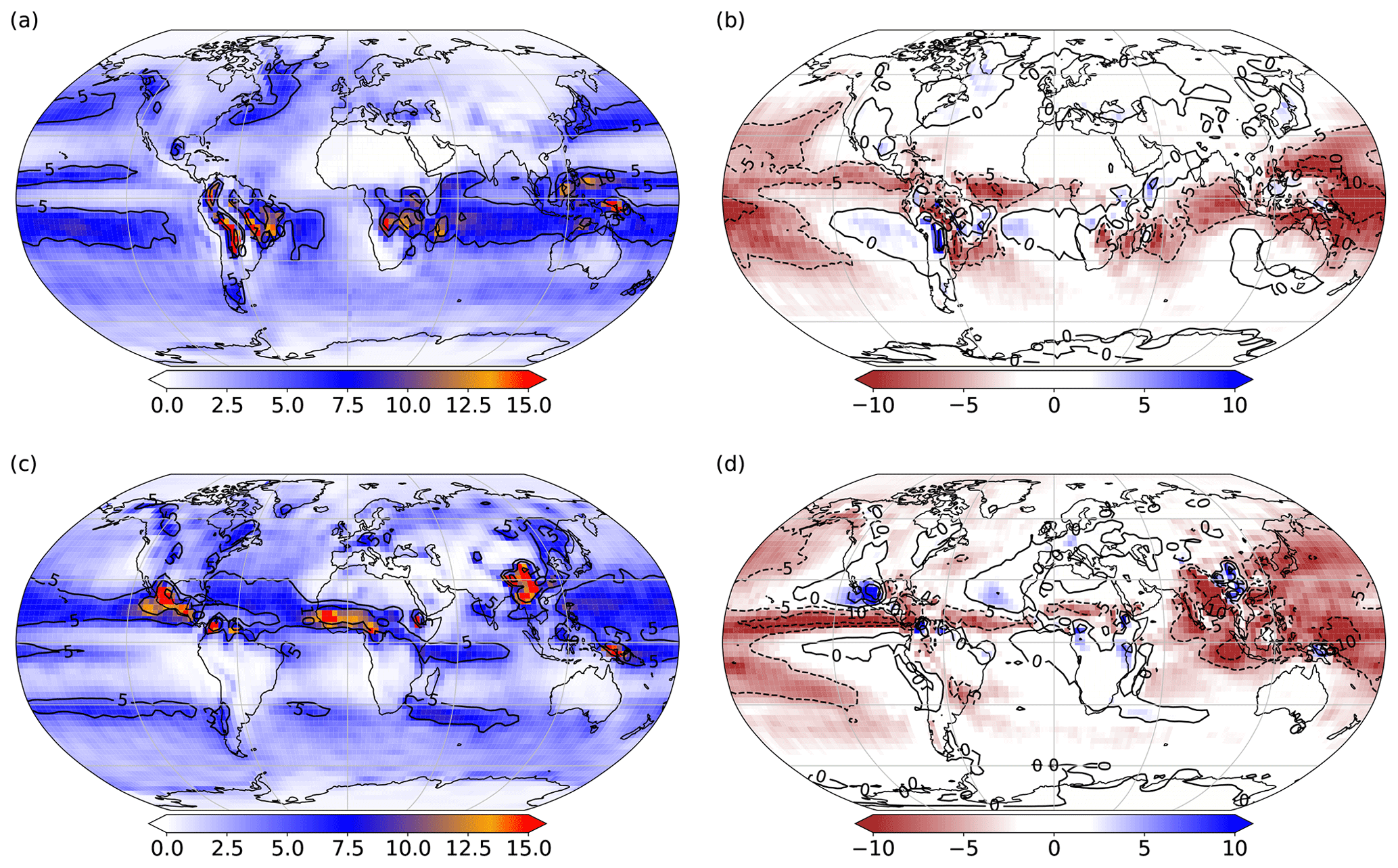
Figure 5Time mean (years 2001–2025) plots from the L35 configuration showing precipitation (mm d−1): (a) DJF, (b) DJF anomaly from 20CR years 1871–1896, (c) JJA and (d) JJA anomaly from 20CR years 1871–1896.
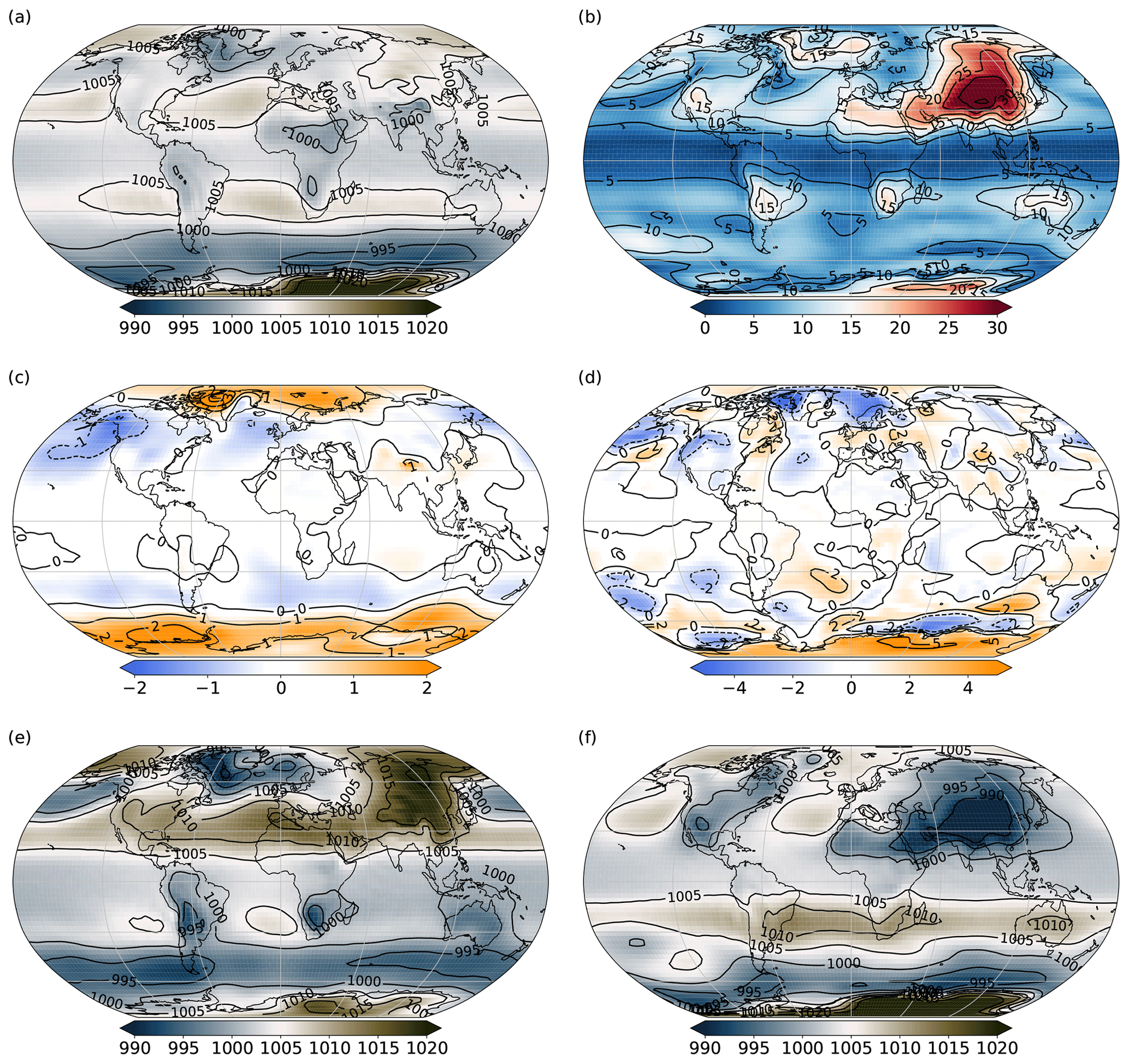
Figure 6Time mean (years 2001–2025) plots showing sea level pressure (mbar): (a) annual mean, (b) seasonal range, (c) difference in sea level pressure for L20–L35 and (d) difference in seasonal range (L20–L35), plus values for the months of (e) January and (f) July from the L35 simulation.
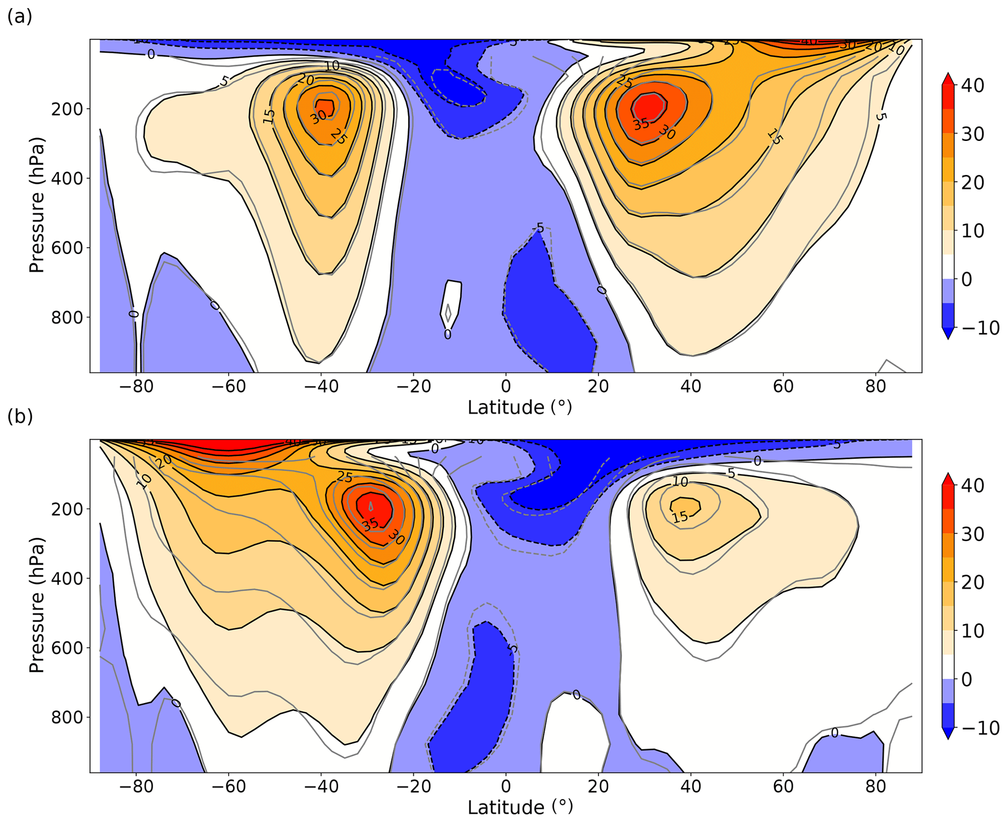
Figure 7Time and zonal mean zonal wind velocities (m s−1) for (a) winter (DJF) mean and (b) summer (JJA) mean. The shading and black contours show the velocities for the L35 simulation, whilst the grey contours show the equivalent contours for the L20 simulation.
Transport through Drake Passage weakens rapidly from an initial value of >160 Sv, and from the year 200 it settles around 110–115 Sv. This is lower than the recent observation-based estimate of 173 Sv (Donohue et al., 2016) or previous estimated values of around 130–140 Sv (e.g. Cunningham et al., 2003) but within the range seen in other coupled climate models (Beadling et al., 2020). Kuhlbrodt et al. (2012) show that the strength of the Antarctic Circumpolar Current (ACC) correlates with the choice of GM thickness diffusion, with lower values of κ yielding stronger ACC transport. The L35 and L20 simulations both use a value of κ=2000. FORTE 2.0 has a stronger ACC than other models that use κ=2000 (see Fig 1b of Kuhlbrodt et al., 2012). It is closer in strength to other models using values of κ=700–1000.
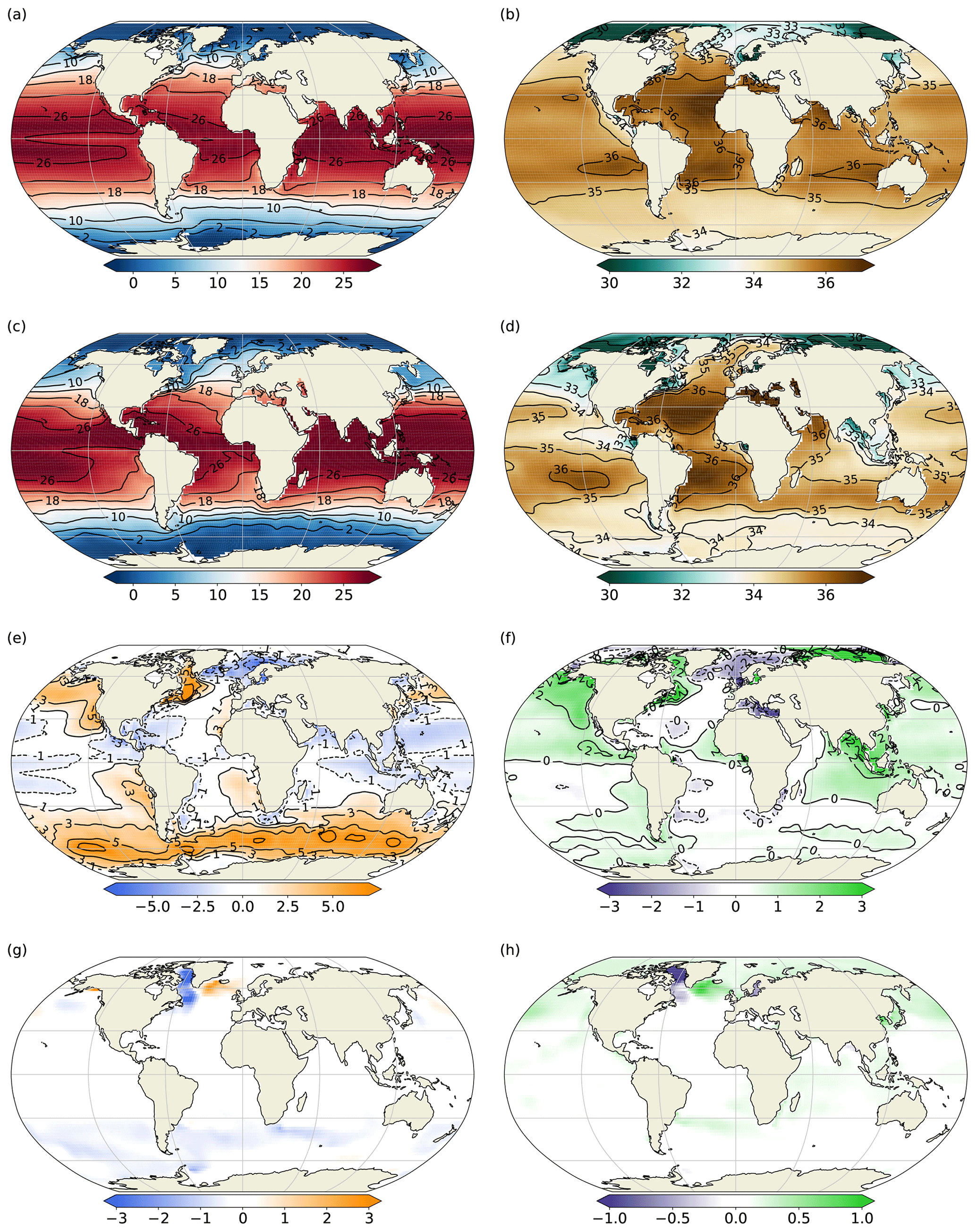
Figure 8Time mean (years 2001–2025) SST and SSS for FORTE 2.0 L35 (a, b) and for EN3 (c, d). Panels (e) and (f) show FORTE 2.0 L35–EN3 SST and SSS anomalies, respectively, whilst panels (g) and (h) show SST and SSS anomalies for L20–L35.

Figure 9Time mean (years 2001–2025) of SSH (m) for (a) FORTE 2.0 L35 and (b) OCCA (2004–2006) climatology. Differences in SSH for (c) L20–L35 and (d) L35–OCCA.
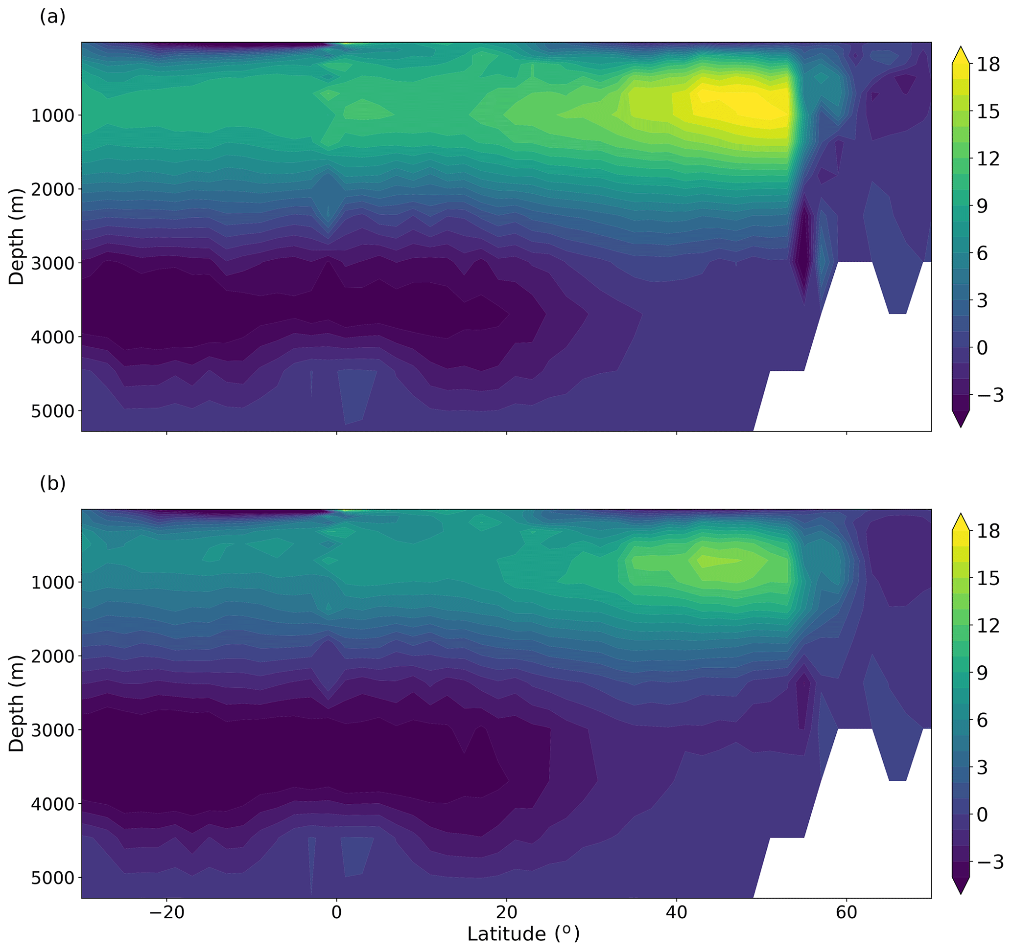
Figure 10AMOC (Sv) as a function of latitude and depth, averaged over the years 1900–2025 of (a) the L35 integration and (b) the L20 integration.
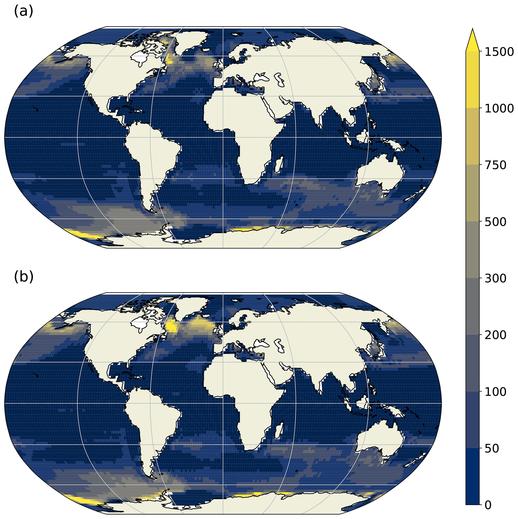
Figure 11Winter mixed layer depths (m) averaged over the years 2000–2025 of (a) the L35 integration and (b) the L20 integration. The Northern (Southern) Hemisphere shows mixed layer depths for the month of March (September). The mixed layer depth is defined as the depth at which a density difference from the top layer of 0.03 kg m−3 occurs.
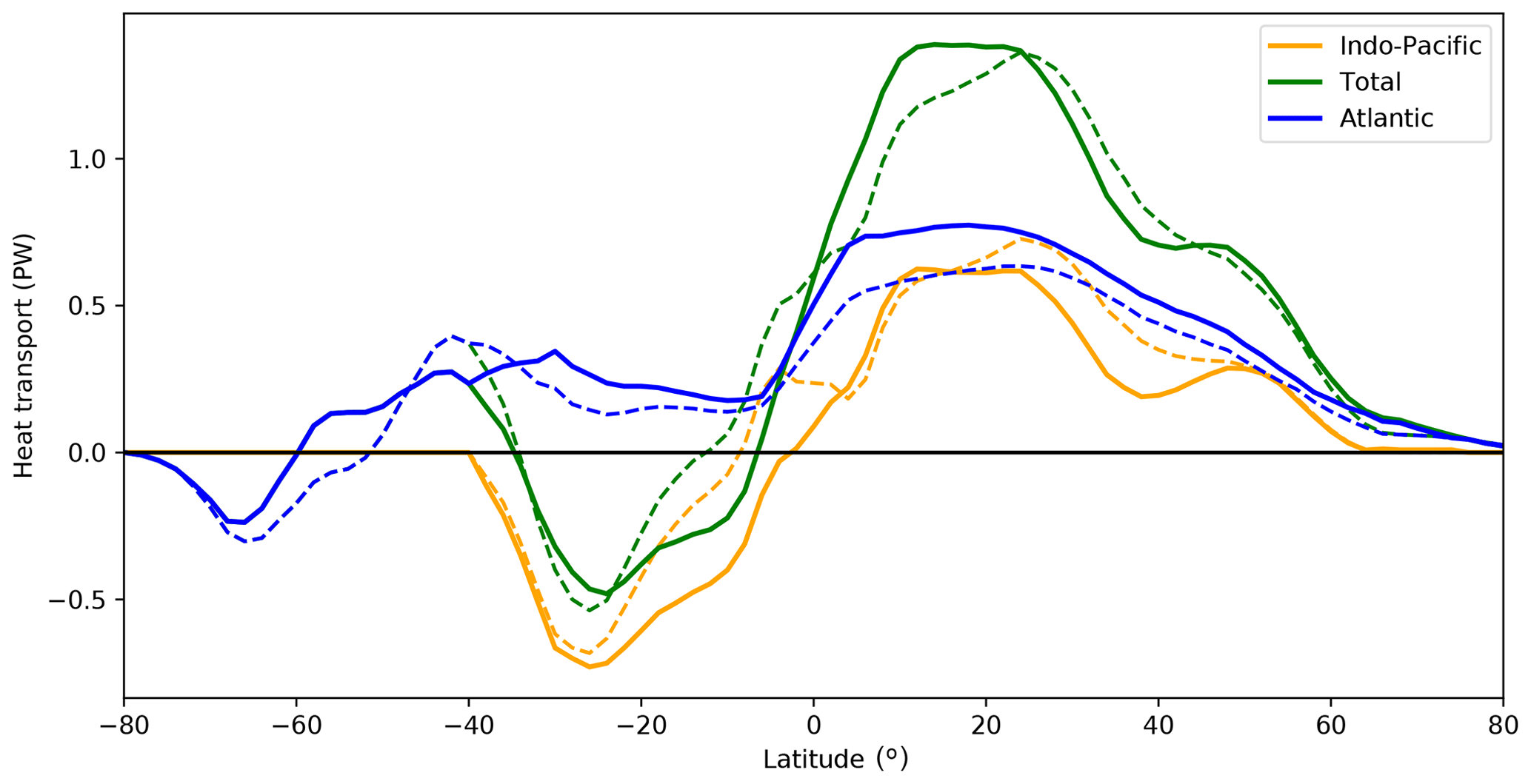
Figure 12Meridional heat transport (PW) as a function of latitude for the global ocean, Atlantic and Indo-Pacific, averaged over the control integration. A five-grid-point smoother has been applied. Solid (dashed) lines show the meridional heat transport for the L35 (L20) simulation.
After the 2000-year spinup, the frequency of output was increased to monthly and a 25-year integration was performed. In this section, the control climate during this 25-year period is presented.
4.1 The atmosphere
Annual time mean surface air temperatures (SATs) in the tropics are 25 ∘C, with some regions over land reaching 30–35 ∘C. The Arctic reaches −20 ∘C, with temperatures over Greenland reaching as low as −40 ∘C and the interior of Antarctica reaches as low as −60 ∘C (Fig. 4a). Anomalies of annual mean SAT from the early years (1871–1896) of the 20th Century Reanalysis (20CR; Compo et al., 2011) are presented in Fig. 4b. FORTE 2.0 performs well at low latitudes, especially over the ocean. There is a pronounced warm anomaly of around 5 ∘C over most of the Southern Ocean, consistent with the positive SST bias shown in Sect. 4.2. A cold SAT anomaly with respect to 20CR also manifests over the Nordic Seas, extending into the Barents Sea. The L20 simulation exhibits very similar annual mean SATs (not shown). Values for L20 are within 1 ∘C of those shown for the L35, except for two regions over the northern Labrador Sea and the Weddell Sea which are cooler in L20 by several degrees. These differences are likely due to the difference in the response of the flux barrier which represents sea ice. The SAT seasonal ranges for FORTE 2.0 and 20CR (1871–1896) are presented in Fig. 4c and d. Seasonal SAT variability over the tropical ocean is low, whilst variations in SAT over land are much higher, reaching 40 ∘C over the Eurasian continent. The seasonal range of FORTE 2.0 compares reasonably well with 20CR throughout most of the low and midlatitudes. However, the seasonal ranges in SAT at high latitudes (both Arctic and Antarctic) are much larger than those in 20CR. Arctic and Antarctic seasonal SAT variability is 40–45 ∘C, with the coldest regions of Antarctica reaching as low as −85 ∘C during July.
Figure 5 shows winter (DJF) and summer (JJA) mean precipitation and anomalies with respect to the 20CR 1871–1896 climatological mean. During DJF (Fig. 5a), regions of high precipitation over the Northern Hemisphere oceanic western boundary currents (up to 6 mm d−1 and extending to northwestern Canada and along the Gulf Stream and western boundary current track in the northwest Atlantic) are evident, as well as high values (10–12 mm d−1) over tropical Africa and South America, Indonesia and over the Intertropical Convergence Zone (ITCZ) in the Atlantic and Pacific oceans. Very low values (0–1 mm d−1) are seen over the polar regions, the subtropical desert regions (terrestrial and oceanic) and (unrealistically) over the equatorial Pacific. During summer (JJA), the ITCZ and the corresponding high levels of rainfall shift northward (Fig. 5c). There is enhanced rainfall due to the Asian summer monsoon, though in FORTE 2.0 it does not extend sufficiently far east. The anomalies with respect to the 20CR 1871–1896 climatological DJF mean (Fig. 5b) show that, particularly over the tropical Pacific, FORTE 2.0 simulates too little rainfall. This is most pronounced over the western tropical Pacific during DJF and also over the northern extent of the ITCZ in the eastern Pacific during JJA (Fig. 5d). A major difference with the observed distribution is the South Pacific ITCZ, which is narrow and predominantly zonal in the model solution, whereas observations show a broader northwest- to southeast-oriented region.
Contours of annual average mean sea level pressure, displayed in Fig. 6a, show the expected bands of high pressure over the subtropical oceans (e.g. the Azores and North Pacific highs) and over the polar regions and low pressure cells at midlatitudes (e.g. Icelandic and Aleutian lows) and over the equatorial regions. The seasonal range is largest over land (Fig. 6b), particularly highlighting the seasonal variability over Siberia. Differences in the annual mean sea level pressure anomalies and seasonal range (L20–L35) are predominantly poleward of 60∘ N and S (Fig. 6c and d). The seasonal range is smaller in L20 over the Labrador and GIN seas and over the high-latitude Southern Ocean. Contours of sea level pressure show the intensification of the surface winds over the midlatitudes in both the Southern Hemisphere and Northern Hemisphere during the winter season (Fig. 6e and f). We note that the Siberian High is not very intense for mean January conditions, and this appears to have the effect of allowing the Icelandic Low to expand and displace eastwards over Scandinavia, resulting in a displacement of the winter North Atlantic Oscillation (NAO) pattern compared with observations (see Sect. 5).
Time mean zonal wind for both summer and winter is shown in Fig. 7 as a function of latitude and pressure. The model exhibits Northern and Southern Hemisphere jet streams at around 40∘ S and 40∘ N at 200 hPa. The southern jet stream exhibits a lower seasonal range (28–36 m s−1) than the northern jet stream (12–36 m s−1). Surface westerlies and easterlies are of the order of ±0–4 m s−1 in the annual mean. The most notable differences between the L20 and L35 configurations occur during JJA, with weaker winds at 60∘ S. The midlatitude cores are also slightly stronger during JJA in L20. At 80∘ S, the zero contour extends down to the surface, indicating a change in the mean wind direction from weak westerlies to weak easterlies.
4.2 The ocean
Annual mean SST (Fig. 8a) shows maximum temperatures in the Indian and tropical Pacific and Atlantic oceans reach 26 ∘C. Compared with the EN3 climatology (Ingleby and Huddleston, 2007, Fig. 8c), there is a cool anomaly of around 1 ∘C throughout the tropics (Fig. 8e). Regions immediately west of the major land masses (coincident with regions of coastal upwelling) show warm SST errors of 2–3 ∘C magnitude, probably arising from a known issue in many coupled climate models related to the poor representation of marine stratocumulus clouds (Gordon et al., 2000). There is a substantial warm bias throughout the Southern Ocean and extending into the southern parts of the Pacific and Indian oceans, likely due to a combination of deficiencies in the physical representations of the ocean dynamics and cloud physics (Hyder et al., 2018). The Nordic Seas are several degrees cooler and up to 1.5 PSU fresher (Fig. 8f) than EN3, possibly due in part to the crude representation of sea ice, and in part due to the inadequate representation of ocean circulation in the Arctic and Nordic seas in a 2∘ resolution ocean model. There is a positive salinity bias of around 3 PSU further east in the Arctic, north of Siberia. Although large, the size of the salinity bias in the Arctic is not uncommon, even for models that do not require a polar island to prevent issues arising from the convergence of the grid at the North Pole (Megann et al., 2010). Annual mean SSS is well represented throughout the Southern Hemisphere ocean, where errors are mainly confined to within ±0.5 PSU (Fig. 8f). Positive biases of the order of 1–1.5 PSU occur in the Bay of Bengal and around the Maritime Continent and the northeast Pacific. The Labrador Sea and the region extending along the US coastline as far south as Cape Hatteras show positive salinity biases between 0.5 and 2 PSU, the latter coincident with a positive temperature bias that exceeds 5 ∘C in a small region that is indicative of the Gulf Stream separating too far north, bringing tropical waters too far north and west. It is worth noting, though, that the L20 simulation exhibits smaller biases in both SST and SSS in the Labrador and Irminger seas (Fig. 8g and h). There is also a slight improvement in the Southern Ocean warm bias in L20 compared with L35. Some of the model biases will arise from the relatively coarse horizontal and vertical resolution and missing physical processes. However, as indicated by the differences between the L20 and L35 simulations, it is likely that a substantial reduction of biases would be achieved with the application of a rigorous calibration methodology such as history matching (Williamson et al., 2015).
Sea surface height (SSH) provides insight into the wind-driven ocean circulation. The SSH from L35 and the Ocean Comprehensible Atlas (OCCA; Forget, 2010) climatology are shown in Fig. 9a and b, respectively. Gyre circulation in all the major ocean basins is highlighted by the contours, along with regions of intensified flow, such as the Gulf Stream, the Kuroshio, and along the northern boundary of the ACC. However, the coarse resolution of the ocean model results in flows that are too broad and diffuse, weakening the SSH gradient across these intensified flows. The North Atlantic subpolar gyre appears constrained to the west of the basin. Slumping of the SSH gradient across the ACC is evident in the anomaly of L35 with respect to OCCA (Fig. 9d) and corresponds to the weak ACC transport shown earlier (Fig. 3). The slope in SSH is also weaker in the North Atlantic and extending into the Nordic Seas. Comparison with L20 (Fig. 9c) shows a slight steepening of the gradient across the ACC in L20, a small reduction in the bias compared with the OCCA climatology.
A latitude depth plot of the AMOC shows a maximum around 50∘ N and at 1000 m depth (Fig. 10). Closely packed streamlines at the high northern latitudes indicate that much of the deep convection occurs abruptly in a narrow latitude band and southward North Atlantic Deep Water transport reaches around 2.5 km depth. The abrupt sinking at the high northern latitudes is characteristic of coarse-resolution ocean models where flow into the Nordic Seas is poorly represented. Winter mixed layer depths in the southern Labrador Sea reach 2500 m in a few grid cells, whilst winter mixed layer depths south of the Denmark Strait, Iceland and the Faroe Bank Channel can reach 1000 m (Fig. 11). Wintertime convection is too shallow in the Nordic Seas, with mixed layer depths reaching 125–150 m in the central and eastern Nordic Seas. The AMOC transport through 30∘ S is 10 Sv in L35 and 6 Sv in L20, and is stronger (∼14 Sv (L35), ∼10 Sv (L20)) at 30∘ N. There is a strong AABW cell (∼6 Sv) centred at 3500 m depth, which weakens to about 2 Sv at 30∘ N. As mentioned earlier, the AABW cell in L20 is slightly stronger, and in Fig. 10 it is shown to extend further north. There is evidence of two-grid-point noise at the Equator, which has been identified previously in Bryan–Cox models (Weaver and Sarachik, 1990). The structure of the AMOC is similar in both the L35 and L20 simulations, with the L20 configuration consistently around 30 % weaker.
Ocean meridional heat transport (OHT) in FORTE 2.0 is around 60 % of that expected based on observational estimates but consistent with the weaker-than-observed volume transport (Fig. 12). Atlantic OHT at 26∘ N is 0.74 PW in L35 and 0.63 PW in L20, whilst observationally derived estimates suggest the current value is closer to 1.3 PW (Johns et al., 2011). Globally, the OHT reaches 1.4 PW, instead of the 2.1±0.3 PW computed by Trenberth and Caron (2001). Over the Southern Ocean (35–65∘ S), OHT is northward, a characteristic seen previously in MOM-based ocean models (de Freitas Assad et al., 2009). This may be related to the strong warm SST bias present over the region at 40–60∘ S (Fig. 8) and its consequent effect on surface heat fluxes.
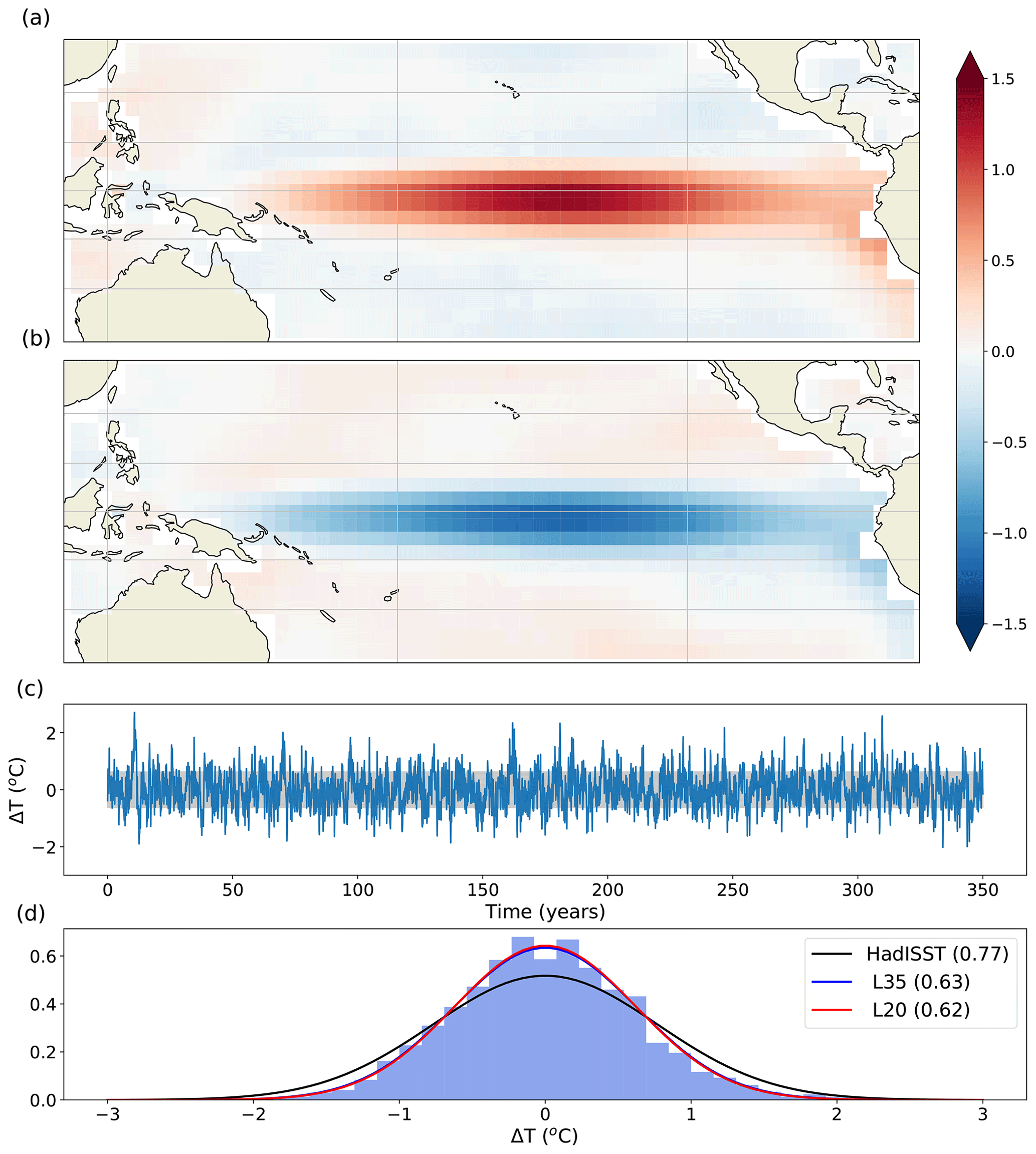
Figure 13Composite anomaly of (a) El Niño events and (b) La Niña events from the L35 simulation. El Niño–Southern Oscillation (ENSO) events are defined as those which exceed ±1 standard deviation anomaly within the Niño 3.4 region. (c) SST anomaly time series and (d) histogram of SST anomaly distribution relative to the mean for the years 1601–1950 from the L35 simulation. The Gaussian curves in panel (d) are fits to the distribution of Niño 3.4 SST anomalies for HadISST (black, Trenberth (2020)), L35 (blue) and L20 (red). The blue and red lines are very close and the red line mostly overlies the blue line. Standard deviations are given in brackets.
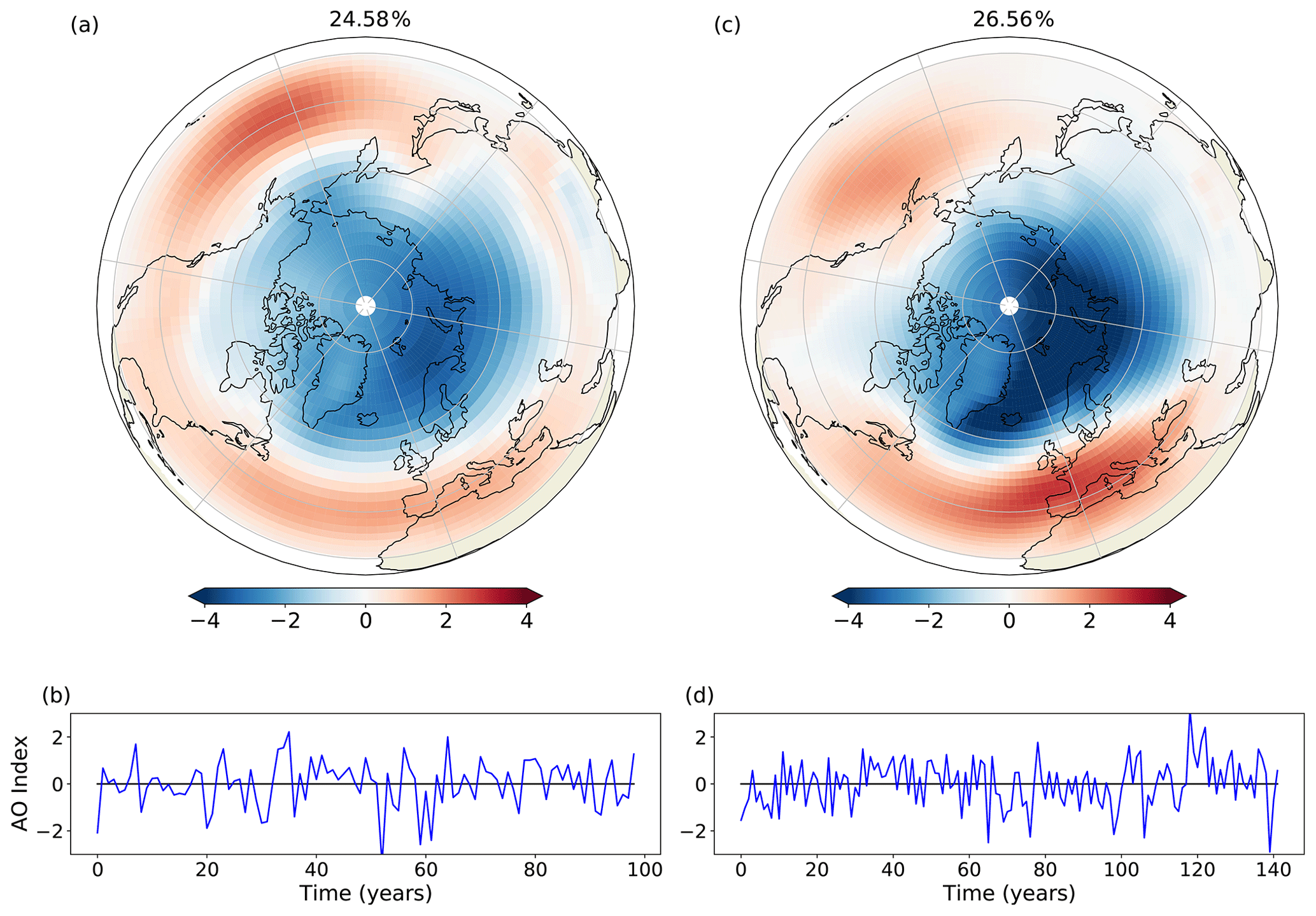
Figure 14The AO as represented by the first EOF and PC computed using deseasoned and latitude-weighted sea level pressure for FORTE 2.0 (a, b) and 20CR (c, d).

Figure 15The NAO as represented by the first EOF and PC computed using deseasoned and latitude-weighted sea level pressure for FORTE 2.0 (a, b) and 20CR (c, d).

Figure 16The SAM as represented by the first EOF and PC computed using deseasoned and latitude-weighted sea level pressure for FORTE 2.0 (a, b) and 20CR (c, d).
A primary aim for any climate model is to adequately reproduce observed modes of climate variability sufficiently well that the model can be used to study the observed phenomena in a variety of contexts. In this section, we present analysis of some of the most important modes using monthly mean ocean output for the years 1600–1950 of the control simulation and daily surface pressure output during the years 1600–1699 of the control integration.
Composites of the SST anomaly during El Niño and La Niña years show the spatial pattern of the anomalies throughout the tropics (Fig. 13a, b). Both phases of the El Niño–Southern Oscillation (ENSO) are weaker than observed, in particular near the eastern boundary. The composite temperature anomaly reaches a maximum of 1 ∘C for the region of 5∘ S–5∘ N, 160–100∘ W, whilst the characteristic region of observed strong SST anomalies near to the coast of Central and South America only reaches 0.7 ∘C and is not strongly connected to the warm anomaly in the central Pacific. This is probably related to the fact that the South Pacific Convergence Zone is too zonal and extends all the way across the Pacific, which is a common feature in coupled climate models (Niznik et al., 2015). The time series of temperature anomalies in the Niño 3.4 region shows a number of strong temperature anomaly events, although the magnitude is in general too small (Fig. 13c, d). We plot the distribution of SST anomalies for the Niño 3.4 region for both model configurations and for HadISST data for the period 1870–2019 (Rayner et al., 2003; Trenberth, 2020). The distribution of the histogram is too narrow compared with observations (Fig. 13d), and there is very little difference between the distributions for the L20 and L35 simulations. In both model configurations, the extreme values extend to around ±2 ∘C (Fig. 13d), whilst observations suggest the extremes should be closer to ±2.5 ∘C.
We also examine the main extratropical modes of variability predicted by FORTE 2.0 in the Northern Hemisphere. We compare 20–90∘ N in an area-weighted empirical orthogonal function (EOF) analysis of the deseasoned and latitude-weighted sea level pressure fields from FORTE 2.0 and 20CR. FORTE 2.0 produces an annular mode structure as the main mode of variability, corresponding to the Arctic Oscillation (AO) in observed data. In agreement with observations (e.g. Thompson and Wallace, 2000; Ambaum et al., 2001), the model reproduces the two midlatitude centres of action over the North Pacific and North Atlantic, with the Pacific centre stronger and the Atlantic centre slightly weaker than those seen in the 20CR and the locations of their maxima displaced westward towards the western half of each ocean basin (Fig. 14). The strength of the Arctic pole in FORTE 2.0 is also weaker than in observations. The NAO is closely related to the AO and is one of the principal modes of atmospheric variability in the North Atlantic sector (Hurrell, 1995). We compute area-weighted EOFs for the NAO over the region of 20–80∘ N, 90∘ W–40∘ E. The first EOF and its accompanying principal component are presented in Fig. 15. In the North Atlantic, there is a good approximation to the NAO pattern, but in FORTE 2.0 the centre of the southern lobe is displaced westward and the northern lobe extends further south over mainland Europe compared with the observed pattern. Again, the principal component suggests more high-frequency variability in observations than in FORTE 2.0.
Similar to the Northern Hemisphere, the Southern Annular Mode (SAM) or Antarctic Oscillation represents the principal mode of climate variability in the Southern Hemisphere. Here, we compute area-weighted EOFs over the region of 20–90∘ S. FORTE 2.0 does not perform as well in the Southern Hemisphere (Fig. 16), with the annular structure significantly weaker over the Pacific and Atlantic sectors. The variance explained by the first EOF is also greatly reduced in FORTE 2.0, approximately half that seen in the 20CR, and this is likely to be linked with the anomalously warm Southern Ocean SST.
We present an assessment of two 2000-year simulations of the FORTE 2.0 coupled climate model: one using the 35σ layer atmosphere including a stratosphere (L35) and one using the 20σ layer atmosphere without a stratosphere (L20). The model integrates from rest and is sufficiently fast to enable studies of multi-centennial climate variability. The model is economic to run and can be adapted and configured to study a wide range of climate questions.
The simulations presented here are not optimally tuned for any specific purpose, but our assessment indicates that FORTE 2.0 is able to simulate a satisfactory climate state and climate variability. Biases that develop in the mean state are comparable to those found in other coupled climate models (Flato et al., 2013) and particularly those of similar complexity and resolution. A small imbalance in the freshwater budget (see Fig. 2) would need to be addressed for studies extending over timescales much longer than several millennia. Modes of climate variability in the Northern Hemisphere are represented well, though there are shortcomings in the Southern Hemisphere variability that are likely related to a strong SST bias over the Southern Ocean. Identifying the cause(s) of such biases is often a complex process in itself (Hyder et al., 2018) and beyond the scope of this current work. A further step would be to rigorously calibrate the model to improve the simulated climate and to better understand the limitations and behaviour of the modelled climate system.
The code, compilation instructions and example run scripts, together with all necessary ancillary files, are accessible at https://doi.org/10.5281/zenodo.4108373 (Blaker et al., 2020). The configuration committed to the Zenodo archive (v2.0.1) is the one used to produce both of the simulations presented in this paper. Readers are advised that there is an error in the IGCM4 compile scripts archived as version 2.0 as linked in the discussion version of this paper. New users are advised to check the latest version of the code, which can be found at https://doi.org/10.5281/zenodo.3632568 (Blaker et al., 2020). Processing of the IGCM4 output requires the BGFLUX programme, a copy of which is accessible from the FORTE 2.0 GitHub repository linked to the Zenodo archive. A comprehensive user guide/manual for FORTE 2.0 does not currently exist. A folder titled “Documentation” has been added to the FORTE 2.0 GitHub repository, and this contains relevant references and copies of technical documents from the original FORTE and component models.
The code and data required to reproduce the figures presented in this paper are provided in the Supplement.
The supplement related to this article is available online at: https://doi.org/10.5194/gmd-14-275-2021-supplement.
ATB, MJ and BS developed the coupled model configuration from versions used in earlier studies. The original coupling of FORTE was performed by BS and RSS. All authors were involved in finalising the configuration presented here. MJ undertook all model simulations. ATB wrote the paper, analysed the output and prepared all tables and figures. All authors edited the paper text.
The authors declare that they have no conflict of interest.
We acknowledge the support of resources provided by the high-performance computing cluster supported by the Research and Specialist Computing Support service at the University of East Anglia. We also acknowledge the support and contributions from colleagues on earlier versions of the code and simulations, most notably Matthew Brand, Craig Wallace and Marc Stringer. We gratefully acknowledge the developers of the software packages PVM and OASIS2.3, both of which are instrumental in the coupling for FORTE 2.0. We thank the editor and reviewers for their contributions. We also acknowledge William Dow, who retrieved and installed FORTE 2.0 from the repository and provided useful feedback to improve the installation instructions.
This research has been supported by the Natural Environment Research Council. Adam T. Blaker, Joël J.-M. Hirschi and Bablu Sinha received support from ACSIS (NE/N018044/1); Bablu Sinha was also supported by SMURPHS (NE/N005686/2). Manoj Joshi was partially funded by SMURPHS (NE/N006348/1).
This paper was edited by Julia Hargreaves and reviewed by two anonymous referees.
Ambaum, M. H. P., Hoskins, B. J., and Stephenson, D. B.: Arctic Oscillation or North Atlantic Oscillation?, J. Climate, 14, 3495–3507, 2001. a
Arakawa, A.: Computational design for long-term numerical integrations of the equations of atmospheric motion, J. Comput. Phys., 1, 119–143, 1966. a
Atkinson, C. P., Wells, N. C., Blaker, A. T., Sinha, B., and Ivchenko, V. O.: Rapid ocean wave teleconnections linking Antarctic salinity anomalies to the equatorial ocean-atmosphere system, Geophys. Res. Lett., 36, L08603, https://doi.org/10.1029/2008GL036976, 2009. a
Beadling, R. L., Russell, J. L., Stouffer, R. J., Mazloff, M., Talley, L. D., Goodman, P. J., Sallée, J. B., Hewitt, H. T., Hyder, P., and Pandde, A.: Representation of Southern Ocean Properties across Coupled Model Intercomparison Project Generations: CMIP3 to CMIP6, J. Climate, 33, 6555–6581, https://doi.org/10.1175/JCLI-D-19-0970.1, 2020. a
Betts, A. K. and Miller, M. J.: The Betts-Miller scheme, in: The Representation of Cumulus Convection in Numerical Models of the Atmosphere, Chapter 9, edited by: Emanuel, K. A. and Raymond, D. J., Amer. Meteor. Soc., Meteor. Mon., 24, 107–121, 1993. a
Blaker, A., Joshi, M., Sinha, B., Stevens, D., Smith, R., and Hirschi, J.: NOC-MSM/FORTE 2.0: FORTE 2.0: a fast, parallel and flexible coupled climate model (Version v2.0.1), Zenodo, https://doi.org/10.5281/zenodo.4108373, 2020. a
Blaker, A. T., Sinha, B., Ivchenko, V. O., Wells, N. C., and Zalesny, V. B.: Identifying the roles of the ocean and atmosphere in creating a rapid equatorial response to a Southern Ocean anomaly, Geophys. Res. Lett., 33, L06720, https://doi.org/10.1029/2005GL025474, 2006. a
Blaker, A., Joshi, M., Sinha, B., Stevens, D., Smith, R., and Hirschi, J.: NOC-MSM/FORTE2.0: FORTE 2.0: a fast, parallel and flexible coupled climate model, Zenodo, https://doi.org/10.5281/zenodo.3632568, 2020. a
Buchan, J., Hirschi, J. J.-M., Blaker, A. T., and Sinha, B.: North Atlantic SST anomalies and the cold North European weather events of winter 2009/10 and December 2010, Mon. Weather Rev., 142, 922–932, https://doi.org/10.1175/MWR-D-13-00104.1, 2014. a
Compo, G. P., S.Whitaker, J., Sardeshmukh, P. D., Matsui, N., Allan, R. J., Yin, X., B. E. Gleason, J., Vose, R. S., Rutledge, G., Bessemoulin, P., Brönnimann, S., Brunet, M., Crouthamel, R. I., Grant, A. N., Groisman, P. Y., Jones, P. D., Kruk, M. C., Kruger, A. C., Marshall, G. J., Maugeri, M., Mok, H. Y., Nordli, Ø., Ross, T. F., Trigo, R. M., Wang, X. L., Woodruff, S. D., and Worley, S. J.: The Twentieth Century Reanalysis Project, Q. J. Roy. Meteor. Soc., 137, 1–28, 2011. a
Cunningham, S. A., Alderson, S., King, B., and Brandon, M.: Transport and variability of the Antarctic Circumpolar Current in Drake Passage, J. Geophys. Res., 108, 8084, https://doi.org/10.1029/2001JC001147, 2003. a
Danabasoglu, G. and McWilliams, J. C.: Sensitivity of the global ocean circulation to parameterizations of mesoscale tracer transports, J. Climate, 8, 2967–2987, 1995. a
de Freitas Assad, L. P., Torres, A. R., Arruda, W. Z., da Silveira Mascarenhas, A., and Landau, L.: Volume and heat transports in the world oceans from an ocean general circulation model, Brazilian J. Geophys., 27, 181–194, https://doi.org/10.1590/S0102-261X2009000200003, 2009. a
Donohue, K. A., Tracey, K. L., Watts, D. R., Chidichimo, M. P., and Chereskin, T. K.: Mean Antarctic Circumpolar Current transport measured in Drake Passage, Geophys. Res. Lett., 43, 11760–11767, https://doi.org/10.1002/2016GL070319, 2016. a
ETOPO5: Global depth and elevation. Technical report, National Geophysical Data Centre, NOAA, US Department of Commerce, Boulder, USA, 1988. a
Eyring, V., Bony, S., Meehl, G. A., Senior, C. A., Stevens, B., Stouffer, R. J., and Taylor, K. E.: Overview of the Coupled Model Intercomparison Project Phase 6 (CMIP6) experimental design and organization, Geosci. Model Dev., 9, 1937–1958, https://doi.org/10.5194/gmd-9-1937-2016, 2016. a
Flato, G., Marotzke, J., Abiodun, B., Braconnot, P., Chou, S. C., Collins, W., Cox, P., Driouech, F., Emori, S., Eyring, V., Forest, C., Gleckler, P., Guilyardi, E., Jakob, C., Kattsov, V., Reason, C., and Rummukainen, M.: Evaluation of climate models, pp. 741–882, edited by: Stocker, T. F., Qin, D., Plattner, G.-K., Tignor, M., Allen, S. K., Doschung, J., Nauels, A., Xia, Y., Bex, V., and Midgley, P. M., Cambridge University Press, Cambridge, UK, https://doi.org/10.1017/CBO9781107415324.020, 2013. a
Forget, G.: Mapping Ocean Observations in a Dynamical Framework: A 2004–06 Ocean Atlas, J. Phys. Oceanogr., 40, 1201–1221, https://doi.org/10.1175/2009JPO4043.1, 2010.
Forster, P. M., Blackburn, M., and Glover, R.: An examination of climate sensitivity for idealised climate change experiments in an intermediate general circulation model, Clim. Dynam., 16, 833–849, 2000. a, b, c
Gargett, A. E.: Vertical eddy diffusivity in the ocean interior, J. Marine Res., 42, 359–393, https://doi.org/10.1357/002224084788502756, 1984. a
Geist, A., Beguelin, A., Dongarra, J., Jiang, W., Manchek, R., and Sunderam, V.: PVM: parallel virtual machine, MIT Press, Cambridge, Massachusetts, 1994. a
Gent, P. R. and McWilliams, J. C.: Isopycnal mixing in ocean circulation models, J. Phys. Oceanogr., 20, 150–155, 1990. a
Gordon, C., Cooper, C., Senior, C., Banks, H., Gregory, J., Johns, T., Mitchell, J., and Wood, R.: The simulation of SST, sea ice extents and ocean heat transports in a version of the Hadley Centre coupled model without flux adjustments, Clim. Dynam., 16, 147–168, 2000. a, b, c
Griffies, S. M.: The Gent-McWilliams skew flux, J. Phys. Oceanogr., 28, 831–841, 1998. a
Griffies, S. M., Gananadesikan, A., Pacanowski, R. C., Larichev, V., Dukowicz, J., and Smith, R.: Isoneutral diffusion in a z-coordinate ocean model, J. Phys. Oceanogr., 28, 805–830, 1998. a
Grist, J. P., Josey, S. A., Sinha, B., and Blaker, A. T.: Response of the Denmark Strait overflow to Nordic Seas heat loss, J. Geophys. Res., 113, C09019, https://doi.org/10.1029/2007JC004625, 2008. a
Haarsma, R. J., Selten, F. M., Opsteegh, J. D., Lenderink, G., and Liu, Q.: A coupled Atmosphere Ocean Sea-ice model for climate predictability studies, Technical Report, KNMI, the Netherlands, 1996. a
Haarsma, R. J., Roberts, M. J., Vidale, P. L., Senior, C. A., Bellucci, A., Bao, Q., Chang, P., Corti, S., Fučkar, N. S., Guemas, V., von Hardenberg, J., Hazeleger, W., Kodama, C., Koenigk, T., Leung, L. R., Lu, J., Luo, J.-J., Mao, J., Mizielinski, M. S., Mizuta, R., Nobre, P., Satoh, M., Scoccimarro, E., Semmler, T., Small, J., and von Storch, J.-S.: High Resolution Model Intercomparison Project (HighResMIP v1.0) for CMIP6, Geosci. Model Dev., 9, 4185–4208, https://doi.org/10.5194/gmd-9-4185-2016, 2016. a
Heuzé, C., Heywood, K., Stevens, D., and Ridley, J.: Changes in Global Ocean Bottom Properties and Volume Transports in CMIP5 Models under Climate Change Scenarios, J. Climate, 28, 2917–2944, https://doi.org/10.1175/JCLI-D-14-00381.1, 2015. a
Hunt, F. K., Hirschi, J. J.-M., Sinha, B., Oliver, K., and Wells, N.: Combining point correlation maps with self-organising maps to compare observed and simulated atmospheric teleconnection patterns, Tellus A, 65, 20822, https://doi.org/10.3402/tellusa.v65i0.20822, 2013. a
Hurrell, J. W.: Decadal trends in the North Atlantic Oscillation regional temperatures and precipitation, Science, 269, 676–679, 1995. a
Hyder, P., Edwards, J. M., Allan, R. P., Hewitt, H. T., Bracegirdle, T. J., Gregory, J. M., Wood, R. A., Meijers, A. J. S., Mulcahy, J., Field, P., Furtado, K., Bodas-Salcedo, A., Williams, K. D., Copsey, D., Josey, S. A., Liu, C., Roberts, C. D., Sanchez, C., Ridley, J., Thorpe, L., Hardiman, S. C., Mayer, M., Berry, D. I., and Belcher, S. E.: Critical Southern Ocean climate model biases traced to atmospheric model cloud errors, Nat. Commun., 9, 3625, https://doi.org/10.1038/s41467-018-05634-2, 2018. a, b
Ingleby, B. and Huddleston, M.: Quality control of ocean temperature and salinity profiles – historical and real-time data, J. Marine Syst., 65, 158–175, https://doi.org/10.1016/j.jmarsys.2005.11.019, 2007. a
Johns, T. C., Durman, C. F., Banks, H. T., Roberts, M. J., McLaren, A. J., Ridley, J. K., Senior, C. A., Williams, K. D., Jones, A., Rickard, G. J., Cusack, S., Ingram, W. J., Crucifix, M., Sexton, D. M. H., Joshi, M. M., Dong, B. W., Spencer, H., Hill, R. S. R., Gregory, J. M., Keen, A. B., Pardaens, A. K., Lowe, J. A., Bodas-Salcedo, A., and Stark, S.: The New Hadley Centre Climate Model (HadGEM1): Evaluation of Coupled Simulations, J. Climate, 19, 1327–1353, 2006. a
Johns, W. E., Baringer, M. O., Beal, L. M., Cunningham, S. A., Kanzow, T., Bryden, H. L., Hirschi, J. J.-M., Marotzke, J., Meinen, C., Shaw, B., and Curry, R.: Continuous, array-based estimates of Atlantic Ocean heat transport at 26.5N, J. Climate, 24, 2429–2449, https://doi.org/10.1175/2010JCLI3997.1, 2011. a
Joshi, M., Stringer, M., van der Wiel, K., O'Callaghan, A., and Fueglistaler, S.: IGCM4: a fast, parallel and flexible intermediate climate model, Geosci. Model Dev., 8, 1157–1167, https://doi.org/10.5194/gmd-8-1157-2015, 2015. a, b, c, d
Killworth, P. D., Stainforth, D., Webb, D. J., and Paterson, S. M.: The development of a free-surface Bryan-Cox-Semtner ocean model, J. Phys. Oceanogr., 21, 1333–1348, 1991. a
Kuhlbrodt, T., Smith, R., Wang, Z., and Gregory, J.: The influence of eddy parameterizations on the transport of the Antarctic Circumpolar Current in coupled climate models, Ocean Model., 52-53, 1–8, 2012. a, b
Levitus, S. and Boyer, T. P.: World Ocean Atlas 1998, Volume 4, Temperature, NOAA Atlas, NESDIS 2, 99 pp., 1998. a, b, c
Levitus, S., Burgett, R., and Boyer, T. P.: World Ocean Atlas 1998, Volume 3, Salinity, NOAA Atlas, NESDIS 3, 99 pp., 1998. a, b
Marsh, R., Hazeleger, W., Yool, A., and Rohling, E. J.: Stability of the thermohaline circulation under millennial CO2 forcing and two alternative controls on Atlantic salinity, Geophys. Res. Lett., 34, L03605, https://doi.org/10.1029/2006GL027815, 2007. a
McCarthy, G., Frajka-Williams, E., Johns, W. E., Baringer, M. O., Meinen, C. S., Bryden, H. L., Rayner, D., Duchez, A., Roberts, C., and Cunningham, S. A.: Observed interannual variability of the Atlantic meridional overturning circulation at 26.5∘ N, Geophys. Res. Lett., 39, L19609, https://doi.org/10.1029/2012GL052933, 2012. a
Meehl, G. A., Covey, C., Delworth, T., Latif, M., McAvaney, B., Mitchell, J., Stouffer, R., and Taylor, K.: The WCRP CMIP3 Multimodel Dataset: A New Era in Climate Change Research, B. Am. Meteorol. Soc., 88, 1383–1394, 2007. a
Megann, A. P., New, A. L., Blaker, A. T., and Sinha, B.: The CHIME coupled climate model, J. Climate, 23, 5126–5150, https://doi.org/10.1175/2010JCLI3394.1, 2010. a, b
Montoya, M., Griesel, A., Levermann, A., Mignot, J., Hofmann, M., Ganopolski, A., and Rahmstorf, S.: The earth system model of intermediate complexity CLIMBER-3-alpha. Part I: description and performance for present-day conditions, Clim. Dynam., 25, 237–263, https://doi.org/10.1007/s00382-005-0044-1, 2005. a
Niznik, M. J., Lintner, B., Matthews, A., and Widlansky, M.: The Role of Tropical–Extratropical Interaction and Synoptic Variability in Maintaining the South Pacific Convergence Zone in CMIP5 Models, J. Climate, 28, 3353–3374, https://doi.org/10.1175/JCLI-D-14-00527.1, 2015. a
Pacanowski, R. C., Dixon, K., and Rosati, A.: The GFDL modular ocean model users guide: version 1.0, GFDL Group Technical Report No. 2, Tech. rep., NOAA/Geophysical Fluid Dynamics Laboratory, Princeton University, Princeton, NJ, variously paged, 1990. a
Rayner, N. A., Parker, D. E., Horton, E. B., Folland, C. K., Alexander, L. V., Rowell, D. P., Kent, E. C., and Kaplan, A.: Global analyses of sea surface temperature, sea ice, and night marine air temperature since the late nineteenth century, J. Geophys. Res., 108, 4407, https://doi.org/10.1029/2002JD002670, 2003. a
Roberts, M. J., Baker, A., Blockley, E. W., Calvert, D., Coward, A., Hewitt, H. T., Jackson, L. C., Kuhlbrodt, T., Mathiot, P., Roberts, C. D., Schiemann, R., Seddon, J., Vannière, B., and Vidale, P. L.: Description of the resolution hierarchy of the global coupled HadGEM3-GC3.1 model as used in CMIP6 HighResMIP experiments, Geosci. Model Dev., 12, 4999–5028, https://doi.org/10.5194/gmd-12-4999-2019, 2019. a
Sellar, A. A., Jones, C. G., Mulcahy, J. P., Tang, Y., Yool, A., Wiltshire, A., O'Connor, F. M., Stringer, M., Hill, R., Palmieri, J., Woodward, S., de Mora, L., Kuhlbrodt, T., Rumbold, S. T., Kelley, D. I., Johnson, R. E. C. E., Walton, J., Abraham, N. L., Andrews, M. B., Andrews, T., Archibald, A. T., Berthou, S., Burke, E., Blockley, E., Dalvi, K. C. M., Edwards, J., Folberth, G. A., Gedney, N., Griffiths, P. T., Harper, A. B., Hendry, M. A., Hewitt, A. J., Johnson, B., Jones, A., Jones, C. D., Keeble, J., Liddicoat, S., Morgenstern, O., Parker, R. J., Predoi, V., Robertson, E., Siahaan, A., Smith, R. S., Swaminathan, R., Zeng, M. T. W. G., and Zerroukat, M.: UKESM1: Description and Evaluation of the U.K. Earth System Model, J. Adv. Model. Earth Syst., 11, 4513–4558, https://doi.org/10.1029/2019MS001739, 2019. a
Shaffrey, L. C., Stevens, I., Norton, W. A., Roberts, M. J., Vidale, P. L., Harle, J. D., Jrrar, A., Stevens, D. P., Woodage, M. J., Demory, M. E., Donners, J., Clark, D. B., Clayton, A., Cole, J. W., Wilson, S. S., Connolley, W. M., Davies, T. M., Iwi, A. M., Johns, T. C., King, J. C., New, A. L., Slingo, J. M., Slingo, A., Steenman-Clark, L., and Martin, G. M.: UK-HiGEM: The New UK High Resolution Global Environment Model. Model description and basic evaluation, J. Climate, 22, 1861–1896, https://doi.org/10.1175/2008JCLI2508.1, 2009. a, b
Sinha, B. and Smith, R.: Development of a fast Coupled General Circulation Model (FORTE) for climate studies, implemented using the OASIS coupler, Tech. rep., Southampton Oceanography Centre, Southampton, UK, Internal Document, No. 81, 67 pp., 2002. a, b, c
Sinha, B., Blaker, A. T., Hirschi, J. J.-M., Bonham, S., Brand, M., Josey, S. A., Smith, R. S., and Marotzke, J.: Mountain ranges favour vigorous Atlantic meridional overturning, Geophys. Res. Lett., 39, L02705, https://doi.org/10.1029/2011GL050485, 2012. a
Smith, R., Dubois, C., and Marotzke, J.: Ocean circulation and climate in an idealised Pangean OAGCM, Geophys. Res. Lett., 31, L18207, https://doi.org/10.1029/2004GL020643, 2004. a, b
Smith, R., Dubois, C., and Marotzke, J.: Global Climate and Ocean Circulation on an Aquaplanet Ocean-Atmosphere General Circulation Model, J. Climate, 19, 4719–4737, 2006. a
Smith, R. S., Gregory, J. M., and Osprey, A.: A description of the FAMOUS (version XDBUA) climate model and control run, Geosci. Model Dev., 1, 53–68, https://doi.org/10.5194/gmd-1-53-2008, 2008. a
Taylor, K., Stouffer, R., and Meehl, G.: An Overview of CMIP5 and the experiment design, B. Am. Meteorol. Soc., 93, 485–498, https://doi.org/10.1175/BAMS-D-11-00094.1, 2012. a
Terray, L., Valcke, S., and Piacentini, A.: The OASIS Coupler User Guide Version 2.3, Tech. Rep. TR/CMGC/99-37, Tech. rep., CERFACS, Toulouse, France, 1999. a
Thompson, D. W. J. and Wallace, J. M.: Annular modes in the extratropical circulation. Part I: Month-to-month variability, J. Climate, 13, 1000–1016, 2000. a
Trenberth, K. E.: The Climate Data Guide: Nino SST Indices (Nino 1+2, 3, 3.4, 4; ONI and TNI), available at: https://climatedataguide.ucar.edu/climate-data/nino-sst-indices-nino-12-3-34-4-oni-and-tni., last access: 10 July 2020. a, b
Trenberth, K. E. and Caron, J. M.: Estimates of meridional atmosphere and ocean heat transports, J. Climate, 14, 3433–3443, 2001. a
Weaver, A. J.: The UVic earth system climate model and the thermohaline circulation in past, present and future climates, IUGG 2003 General Assembly of the International Union of Geodesy and Geophysics No23, Sapporo, Geophysical monograph ISSN 0065-8448 CODEN GPMGAD, 150 (416 p.), 279–296, 2004. a
Weaver, A. J. and Sarachik, E. S.: On the importance of vertical resolution in certain ocean general circulation models, J. Phys. Oceanogr., 20, 600–609, 1990. a
Weaver, A. J., Eby, M., Augustus, F. F., and Wiebe, E. C.: Simulated influence of carbon dioxide, orbital forcing and ice sheets on the climate of the Last Glacial Maximum, Nature, 394, 847–853, 1998. a
Webb, D. J.: An ocean model code for array processor computers, Comput. Geosci., 22, 569–578, 1996. a, b
Webb, D. J., de Cuevas, B. A., and Richmond, C. S.: Improved Advection Schemes for Ocean Models, J. Atmos. Ocean. Tech., 15, 1171–1187, 1998. a
Williamson, D., Blaker, A. T., Hampton, C., and Salter, J.: Identifying and removing structural biases in climate models with history matching, Clim. Dynam., 45, 1299–1324, https://doi.org/10.1007/s00382-014-2378-z, 2015. a
Wilson, C., Sinha, B., and Williams, R. G.: The effect of ocean dynamics and orography on atmospheric storm tracks, J. Climate, 22, 3689–3702, https://doi.org/10.1175/2009JCLI2651.1, 2009. a
Wu, J.: Wind-Stress Coefficients over Sea Surface near Neutral Conditions - A Revisit, J. Phys. Oceanogr., 10, 727–740, 1980. a
Zhong, W. Y. and Haigh, J. D.: Improved broad-band emissivity parameterization for water vapor cooling calculations, J. Atmos. Sci., 52, 124–148, 1995. a